Draft version May 9, 2016Preprint typeset using LATEX style emulateapj v. 12/16/11

FALSE POSITIVE PROBABILITIES FOR ALL KEPLER OBJECTS OF INTEREST:1284 NEWLY VALIDATED PLANETS AND 428 LIKELY FALSE POSITIVES

Timothy D. Morton1, Stephen T. Bryson2, Jeffrey L. Coughlin2,3, Jason F. Rowe4, Ganesh Ravichandran5,Erik A. Petigura6,7, Michael R. Haas2, and Natalie M. Batalha2

Draft version May 9, 2016

ABSTRACT

We present astrophysical false positive probability calculations for every Kepler Object of Interest(KOI)—the first large-scale demonstration of a fully automated transiting planet validation procedure.Out of 7056 KOIs, we determine that 1935 have probabilities <1% to be astrophysical false positives,and thus may be considered validated planets. 1284 of these have not yet been validated or confirmedby other methods. In addition, we identify 428 KOIs likely to be false positives that have not yetbeen identified as such, though some of these may be a result of unidentified transit timing variations.A side product of these calculations is full stellar property posterior samplings for every host star,modeled as single, binary, and triple systems. These calculations use vespa, a publicly availablePython package able to be easily applied to any transiting exoplanet candidate.

1. INTRODUCTION

The Kepler mission has revolutionized our understand-ing of exoplanets. Among many other important dis-coveries, Kepler has identified several previously unsus-pected features of planetary systems, such as the preva-lence of planets between the size of Earth and Neptune,and a population of very compact multiple-planet sys-tems. And perhaps most notably, it has enabled for thefirst time estimates of the occurrence rates of small plan-ets (&1 R⊕) out to orbits of about one year (e.g. Petiguraet al. 2013; Foreman-Mackey et al. 2014; Burke et al.2015). It is important to remember, however, that theserevolutionary discoveries depend intimately on anotherrevolution—how to interpret transiting planet candidatesignals in the absence of unambiguous positive confirma-tion of their veracity.

Before Kepler, every survey searching for transiting ex-oplanets demanded that a candidate signal be verified asa true planet via radial velocity (RV) measurement ofits mass. This would involve a series of follow-up ob-servations in order to weed out astrophysical false posi-tive scenarios—typically stellar eclipsing binaries in var-ious configurations. However, following this model hasbeen largely impossible for Kepler because of the quan-tity and character of the planet candidates (thousandsof mostly small-planet candidates around relatively faintstars). There have been a small number of Kepler planetswith masses measured by RVs (e.g., Marcy et al. 2014;Santerne et al. 2015), and significantly more that havebeen confirmed as planets by measurement of transit tim-

1 Department of Astrophysical Sciences, Princeton University,4 Ivy Lane, Princeton, NJ 08544, USA, tdm@astro.princeton.edu

2 NASA Ames Research Center, M/S 244-30, Moffett Field,CA 94035, USA

3 SETI Institute, 189 Bernardo Ave, Mountain View, CA94043, USA

4 Departement de Physique, Universite de Montreal, Montreal,QC, Canada, H3T 1J4

5 Department of Computer Science, Columbia University, 1214Amsterdam Ave, New York, NY 10027

6 California Institute of Technology, Pasadena, CA 91125,USA

7 Hubble Fellow

ing variations (TTVs) in multi-planet systems (e.g., Fordet al. 2012; Steffen et al. 2012; Fabrycky et al. 2012; Stef-fen et al. 2013; Jontof-Hutter et al. 2015), but this stillleaves the vast majority of candidates inaccessible to dy-namical confirmation.

This situation has inspired the development of proba-bilistic validation as a new approach to evaluating transitcandidates. The principle of probabilistic validation is todemonstrate that all conceivable astrophysical false pos-itive scenarios are negligibly likely to be the cause of atransit candidate signal compared to the explanation of aplanet transiting the presumed target star. The BLENDERmethod pioneered this approach and has validated manyKepler candidates (e.g., Borucki et al. 2012; Kippinget al. 2014; Torres et al. 2015). More recently, the PASTISanalysis suite has been introduced (Dıaz et al. 2014)and used to validate both Kepler and CoRoT candidates(e.g., Santerne et al. 2014; Moutou et al. 2014). An al-ternative validation approach for candidates in multiple-planet systems has also been applied to a large number ofKepler systems based on the general argument that it isunlikely to see multiple false-positive signals in the sameKepler light curve (Lissauer et al. 2012), resulting result-ing in validations of over 800 planets with 99% confidence(Lissauer et al. 2014; Rowe et al. 2014). This method-ology differs from the BLENDER/PASTIS approach in twosignificant ways: (a) it is applicable only to planets inmulti- planet systems, and (b) it relies on broad-brushgeneral arguments rather than analyzing the details ofcandidate signals individually.

While they have both proven useful for the purposesof validating individual candidates of particular inter-est, neither BLENDER nor PASTIS is designed for fullyautomated batch processing of large numbers of candi-dates. Morton (2012) describes a computationally sim-pler planet validation procedure designed for exactly sucha purpose, based on the idea of describing eclipse lightcurves as simple trapezoids and simulating realistic pop-ulations of astrophysical false positives. This procedurehas also been used in the literature to validate a num-ber of Kepler planets (e.g., Muirhead et al. 2012; Daw-son et al. 2012; Swift et al. 2013), and has also been

2 Morton et al.

applied to a number of candidates found by the K2 mis-sion (Montet et al. 2015; Becker et al. 2015). The codethat implements this procedure is publicly available inthe Python module vespa8 (Morton 2015b).

This work presents results of applying vespa en masseto the entire Kepler catalog. This is both the first timethat most Kepler candidates have been individually an-alyzed to assess false positive probability and the firsttime that a detailed automated planet validation calcu-lation has been applied on such a large scale. Section 2describes the methods used, Section 3 describes the dataset, Section 4 presents the results, Section 5 comparesthese results with observational studies, and Section 6contains concluding remarks.

2. METHODS

In this work, we apply the fully automated FPP-computing procedure described in Morton (2012, here-after M12) to 7056 Kepler Objects of Interest (KOIs; seeSection 3 for details). While we refer the reader to M12for a detailed description of the method, we outline itbriefly in this section.

2.1. False Positive Probabilities

The basic idea of vespa is to assign probabilities to dif-ferent hypotheses that might describe a transiting planetcandidate signal. If {Hi} is the set of all considered hy-potheses, the probability for any given model i is

Pr (Hi) =πiLi∑

j

πjLj

, (1)

where πi is the “hypothesis prior” and Li is the “hy-pothesis likelihood”9 The prior represents how intrinsi-cally probable the hypothesized scenario is to exist, andthe likelihood represents how closely the shape of the ob-served transit signal matches with the expected shape ofa signal produced by the hypothesis.

The vespa procedure models an eclipse signal as asimple trapezoid, parametrized by depth δ, total du-ration T , and shape parameter T/τ , where τ is the“ingress/egress” duration (such that a completely V-shaped transit has T/τ = 2). For the transit signal beingevaluated, the joint posterior probability density func-tion (PDF) of these shape parameters is sampled withMarkov Chain Monte Carlo (MCMC), using the emceesampler (Foreman-Mackey et al. 2013). This allows thelikelihood for each hypothesis to be determined by sim-ulating a physically realistic population of the hypothe-sized astrophysical scenario and using this population todefine the PDF for the trapezoidal parameters under thehypothesis. The likelihood is then

Li =

∫psig (θ) pi (θ) dθ, (2)

where θ is the vector of trapezoidal shape parameters,psig is the posterior PDF of the signal, and pi is the PDF

8 https://github.com/timothydmorton/vespa9 This factor is more widely known as the “Bayesian evidence”

or “marginalized likelihood”; Morton (2014) argues for the term“hypothesis likelihood,” as it can be clarifying to think of it thatway.

for the parameters under hypothesis i.10 The hypothe-ses supported by vespa are the following: unblendedeclipsing binary (EB), hierarchical-triple eclipsing binary(HEB), chance-aligned background/foreground eclipsingbinary (BEB), and transiting planet (Pl).11 In this work,we also implement “double-period” versions of each ofthe stellar false positive scenarios, acknowledging thepossibility that if an eclipsing binary has similar primaryand secondary eclipse depths, then it might be mischar-acterized as a primary-only transiting planet signal attwice the orbital period (especially if diluted). We notethat the determination of the diluted eclipse depth ofall these blended scenarios assumes that the light fromthe blended system is fully contained within the target’sphotometric aperture. That is, these scenarios do notaccount for the possibility that only a small fraction ofthe light from a nearby contaminating star might be inthe aperture, many of which have already been identifiedvia other methods Bryson et al. (2013); Coughlin et al.(2014).

Observational constraints are incorporated in twodifferent ways. First, photometric (or spectro-scopic/asteroseismic) measurements of the target star arefolded into the population simulations of each hypothe-sis (see Section 2.2). All other constraints are applied tonarrow down which simulated instances of each scenariomay be counted in the final prior and likelihood evalula-tions; for example, only blended eclipsing binaries withsecondary eclipse depths shallower than the observed lim-its contribute to the construction of the pi trapezoidalshape parameter PDF. For the “double-period” scenar-ios, we require the primary and secondary eclipse sig-nals to have depths within 3-σ of each other, where σ isdefined as the fitted uncertainty in the trapezoid-modeldepth of the candidate signal.

The steps vespa takes to calculate the FPP of a transitsignal are thus as follows:

1. Generate posterior samples for the transit signalunder the trapezoid model, using MCMC.

2. Generate population simulations for each hypothe-sis scenario being considered (conditioned on avail-able observations of the target star; see Sec-tion 2.2).

3. Fit each simulated eclipse in each scenario with atrapezoid model (using least-squares optimization).

4. Evaluate priors and likelihoods for each hypothe-sis, taking into account all available observationalconstraints.

5. Use Equation (1) to calculate the posterior proba-bility for each scenario.

10 Li may be seen to be the “evidence” or “marginalized likeli-hood” of the trapezoidal model under hypothesis i, with psig beingthe likelihood and pi being the prior, integrated over the θ pa-rameter space. But for clarity, and for continuity with previouspublications, we continue to call Li the “likelihood” for hypothesisi.

11 We note that we do not consider “blended transiting planet”false positive scenarios, either due to physically associated orchance-aligned companions. See Section 4.6 for more discussion.

False Positive Probabilities for all KOIs 3

To quantify uncertainty due to the Monte Carlo na-ture of this procedure, vespa is also able to repeat thesecalculations any desired number of times by bootstrapresampling (with replacement) of the simulated popu-lations, and recalculating the likelihoods based on theresampled populations. This mitigates the chances forrare outliers in a simulation to significantly affect thecalculated FPP.

We note that a built-in weakness of model selectionis that it assumes that the set of models being consid-ered is comprehensive. This could in principle lead to asituation where one model is strongly preferred over allother models, but even that model is a poor explanationof the data—in this work, this could lead to improperlyvalidated planets. There are two general strategies to tryto address this issue. The first is to somehow quantifythe absolute goodness-of-fit of the models, and requirethat a validated planet pass some threshold test. Theother strategy, that we adopt here, is to expand the setof models to be more comprehensive. In order to do this,we introduce two artificial models: “boxy” and “long.”The “boxy” likelihood function is a step function at someminimum value of T/τ (zero below this threshold, andconstant above), and constant throughout the space ofthe other trapezoidal parameters. Similarly, the likeli-hood of the “long” model is a step function at some min-imum threshold value of duration T . These thresholdsare set relative to the simulated trapezoidal shapes of theplanet model: the T/τ threshold is the maximum valuefrom the simulated planet population, and the T thresh-old is the 99% percentile of simulated planet populationvalues. We also choose the model priors for these arti-ficial models to be low, reflecting that we expect only asmall number of signals to be unexplained by any of theastrophysical scenarios: the number that we choose foreach of these models is 5 × 10−5, corresponding to anexpectation that there may be ∼10 such signals amongthe ∼200,000 Kepler targets.

2.2. Stellar Properties

The most substantial difference between the currentimplementation of vespa and the procedure documentedin M12 is how stellar properties are treated. Previously,either the target star’s mass and radius were explicitlyprovided, or they were randomly generated according tothe stellar population expected along the line of sightby the TRIdimensional modeL of thE GALaxy (TRI-LEGAL) Galactic stellar population synthesis tool, butconstrained to agree with some observed color(s) of thestar (e.g. J − K), to within some specified tolerance.This strategy was used both to generate the host starsfor the transiting planet model and the binary and triplestars for the EB and HEB false positive models.

The new method now used by vespa uses theisochrones Python module (Morton 2015a) to fold inobservational constraints on the host star. At its core,isochrones performs 3-D linear interpolation in mass–[Fe/H]–age parameter space for a given stellar modelgrid. This method of stellar modeling for FPP calcu-lation debuted in Montet et al. (2015) and is explainedthere in more detail. Instead of randomly generatingstars (or binary or triple systems of stars) from a pre-defined distribution and culling them to approximatelyagree with observed colors, all available constraints on

TABLE 1Priors used in stellar property fits

Parameter Prior

Primary mass MA ∝M−2.35A , MA > 0.1

Secondary mass MB ∝ (MB/MA)0.3, 0.1 <= MB < MA

Tertiary mass MC ∝ (MC/MA)0.3, 0.1 <= MC < MBAge [Gyr] U(1, 15) a

[Fe/H] 0.80.15N (0.016, 0.15) + 0.2

0.22N (−0.15, 0.22) b

AV [mag] U(0, AV,max) c

Distance d ∝ d2

a The age range for the Dartmouth stellar model grids used.b Double-Gaussian fit to measured local stellar metallicity distribution(Hayden et al. 2015; Casagrande et al. 2011).c Maximum allowed value is the Galactic extinction at infinity calcu-lated along the star’s line of sight, according to Schlegel et al. (1998).

the target star are used to condition a direct fit of ei-ther a single–, binary–, or triple–star model to the Dart-mouth grid of stellar models (Dotter et al. 2008; Fei-den et al. 2011). This fit is done using multi-modalnested sampling, implemented with MultiNest (Ferozet al. 2009, 2011, 2013), via the PyMultiNest wrapper(Buchner et al. 2014). Monte Carlo samples of stellarproperties for the population simulations are then drawndirectly from these posterior samples.

As a result, vespa creates full posterior samplings ofthe physical properties of the host star, modeled as a sin-gle, binary, and triple star system, as a by-product of theFPP calculation. Parameters directly fitted for in thisprocess are stellar mass, age, [Fe/H], AV extinction, anddistance. For binary and triple fits, secondary and/ortertiary mass parameters are added, with all other pa-rameters assumed to be the same among all components.Photometric observations upon which these fits are con-ditioned are assumed to be the sum of all components.If spectroscopic and/or asteroseismic measurements areused (e.g., constraints on effective temperature or stel-lar surface gravity), they are assumed to relate to onlythe primary star. Priors used in these fits are listed inTable 1—notably, we use a prior on [Fe/H] based on adouble-Gaussian fit to the local metallicity distribution(Hayden et al. 2015; Casagrande et al. 2011). Posteriorchains of all other stellar parameters of interest (e.g.,temperature, surface gravity, radius, etc.) are derivedfrom the chains of fitting parameters by evaluting thestellar models using isochrones.

3. DATA AND CONSTRAINTS

The goal of this work is to calculate the FPP for everyKOI, regardless of classification as CONFIRMED, CAN-DIDATE, or FALSE POSITIVE. As such, we begin witha list of 7470 KOIs from the Q1-Q17 DR24 table at theNASA Exoplanet Science Institute (NExScI) ExoplanetArchive (the most recent available uniform catalog). Wethen gather ancillary data and constraints from varioussources in order to enable the vespa calculation:

1. The RA/Dec coordinates of each star from the Ke-pler Input Catalog (KIC).

2. grizJHK photometry from the KIC, with grizbands corrected to the Sloan Digital Sky Survey(SDSS) photometric scale according to Pinson-neault et al. (2012).

4 Morton et al.

3. Stellar Teff , [Fe/H], and log g values and uncertain-ties from the Huber et al. (2014) stellar propertiescatalog, if the provenance of these values is fromspectroscopy or asteroseismology.

4. Detrended Kepler photometry used for the MCMCmodeling of Rowe et al. (2015), along with informa-tion about individually fitted transit times, whereavailable.

5. Best-fit Rp/R? from the Rowe et al. (2015) MCMCanalysis.

6. Centroid uncertainty information from the NExScIExoplanet Archive: we assume that the allowed“exclusion” radius for a blend scenario is 3× theuncertainty in the fitted centroid position (thekoi_dicco_msky_err column in the Archive ta-ble). We floor this value at 0.′′5, to prevent un-realistically small exclusion radii. If this quantityis not available from the Archive we set a defaultexclusion radius of 4′′.

7. The maximum secondary eclipse depth allowed bythe Kepler photometry. This quantity is derived bysearching the phased-folded KOI light curve for thedeepest signal at any other phase other than thatof the primary transit. This “model-shift unique-ness test” is described in both Section 3.2.2 of Roweet al. (2015) and Coughlin et al. (2015a), and thevalues of these metrics for the Q1-Q17 DR24 re-lease will soon be published (Coughlin et al. 2015,submitted). The maximum secondary depth we useis

δmax = δsec + 3σsec, (3)

where δsec is the fitted depth and σsec is the un-certainty on that depth (including red noise). Asthe DR24 pipeline uses two different detrendingmethods, we calculate δmax and σmax using bothmethods and take the maximum between the two.When these metrics are not available for a par-ticular KOI, we default to 10× the uncertaintyin the Kepler pipeline measured transit depth(koi_depth_err1).

As explained in the vespa documentation, we first spec-ify this ancillary data in a star.ini and fpp.ini file foreach KOI, and then for each we run the command-linescript calcfpp. This end-to-end calculation (which in-cludes the isochrones fits for single-, double-, and triple-star models) takes approximately 30 minutes per KOI ona single core, allowing the entire set to be calculated inapproximately one day on the Princeton Univeristy “Ti-gress” computing cluster, using 200 cores.

4. RESULTS

The results of the vespa calculations are presented inTable 5 and Table 6, and are discussed in the followingsubsections.

4.1. Stellar Properties

As discussed in Section 2.2, vespa fits for stellar prop-erties as part of its FPP–calculating procedure, using the

isochrones package. Thus, we obtain posterior sam-plings of the physical properties of each KOI as a sideeffect of this batch calculation, a result of general inter-est independent of FPP. Table 5 presents summarizedresults of these single–star fits. While vespa also fitsdouble– and triple–star models for each KOI, these areof less general interest and so we do not present themseparately.

FIG. 1 and FIG. 2 compare the estimated effective tem-peratures, metallicities, and radii derived in this workto those independently determined for (or compiled by)the official Kepler stellar properties catalog (Huber et al.2014, hereafter H14). While there is largely generalagreement, there are also some discrepancies, highlight-ing some difficulties of estimating physical stellar prop-erties.

In particular, we note that for stars which H14 list asTeff < 4000 K, isochrones predicts systematically hottertemperatures. Many of the H14 properties for these starsare taken from Dressing & Charbonneau (2013, D13).Those properties were determined by trying to matchthe grizJHK photometry of a grid of model stars fromthe Dartmouth models, supplemented by some interpo-lation. D13 also imposed priors on [Fe/H] and the heightof stars above the plane of the Galaxy. To validate theirmethodology, D13 compare their results for 26 nearbystars to the masses predicted for those stars by combin-ing parallax measurements with the Delfosse et al. (2000)relation between mass and absolute K-band magnitude.While they find general good agreement, D13 does notethat their masses are on average about 5% lower thanthe Delfosse-predicted masses. Our estimated masses forthese stars are typically ∼10-15% higher than those es-timated by D13.

The same data (grizJHK photometry) and the samestellar models (Dartmouth) were used for both this workand D13, raising the question of the origin of the sys-tematic differences between these methods. The primaryorigin of this discrepancy appears to be the fact thatisochrones performs a full multi-modal posterior ex-ploration of the stellar parameter space, marginalizingover the unknown AV extinction in the process, whileD13 uses rather a fixed 1 mag of V -band extinction per1000 pc and selects the maximum-likelihood match to thegrid of models. As we allow for a maximum extinction upto the measured AV extinction at infinity, not explicitlytied to distance, this typically allows for slightly hotterstars with slightly more extinction than was permittedby Dressing & Charbonneau (2013).

The other significant discrepancy between theisochrones results and H14 is among evolved stars,as seen in the lower panel of FIG. 2. Many of thesestars have densities measured via asteroseismology, andisochrones does not unambiguously identify all of themas evolved. However, it should be noted that we do infact identify over half of them as probably significantlyevolved—this is made possible by the multi-modal poste-rior sampling of MultiNest used by isochrones. In ad-dition, as the middle panel of FIG. 2 shows, even for starsnot positively identified as evolved by H14, isochronesoften allows for a significant range of stellar radius—also desirable behavior, as H14 estimates the propertiesfor many of these using only broad-band photometryas well, which means their true nature is not securely

False Positive Probabilities for all KOIs 5

known. The need for caution when estimating the radiiof KOI host stars has also been emphasized by Bastienet al. (2014), who find from photometric “flicker” mea-surements that a significant number of FGK KOI hostsmay be slightly evolved.

We emphasize that stellar parameter estimation is notthe central goal of this work, nor are the FPP results verysensitive to the exact estimated stellar properties. Theexception to this would be if the stellar density estimateis significantly mis-estimated, which would be the case ifa star is not properly identified as evolved. However, wenote that of the 730 KOIs with host stars >2R� at theNExScI Archive, 502 of them already have FALSE POSI-TIVE designations; additionally, Sliski & Kipping (2014)find a large false positive rate for KOIs with evolved hoststars. Given all of these considerations, we believe thatpotential systematic issues with stellar property deter-minations in various corners of parameter space do notstrongly affect the main results, which are the astrophys-ical false positive probabilities of thousands of KOIs.

4.2. False Positive Probabilities

Of the 7470 KOIs in the Q1-Q17 DR24 table at theNExScI Exoplanet Archive, vespa successfully calculatesthe FPP for 7056. Section 4.7 contains detailed expla-nations of the failure reasons for the 414 KOIs for whichwe do not present vespa results. FPPs and their uncer-tainties are determined as the mean and standard de-viations of 10 bootstrap recalculations of the initiallysimulated populations for each KOI (as described in Sec-tion 2.1). These results are listed in Table 6. The medianfractional FPP uncertainty for KOIs with 0.001 < FPP< 0.1 (within an order of magnitude of the validationthreshold) is about 12%, and this distribution is shownin FIG. 3.

In order to properly interpret these results, it is nec-essary to understand the range of applicability of thevespa calculation. First of all, this method selects be-tween different specific explanations for the transit-likesignal, and cannot comment on whether the signal mightbe caused by stellar variability or an instrumental falsealarm. Thus, vespa results on low signal-to-noise ratio(SNR) candidates that are not clearly transit-like mustbe viewed with caution. This being said, the reason forincluding the artificial “boxy” and “long” models in themodel selection calculation (Section 2.1) is to flag signalsthat do not fit well with any of the astrophysical eclipsemodels—in fact, the “long” model is preferred (> 50%)by 526 KOIs that are already dispositioned as FALSEPOSITIVE.

Additionally, an important constraint used in the FPPcalculation is the allowed sky area inside which a blendedfalse positive may live. As described in Section 3, thisvalue is taken to be three times the uncertainty on the fit-ted centroid position from the pixel-level data. However,many KOIs have already been identified to be blended bi-nary false positives displaced from the target star. Someof these are found by detecting significant centroid off-sets in the pixel-level data—in these cases, vespa treat-ing the confusion radius simply as the uncertainty inthe centroid position will clearly give a misleading re-sult. Other displaced false positives have been identi-fied as originating from displaced stars by finding KOIswith matching periods and epochs (Coughlin et al. 2014),

TABLE 2Mean FPPs of candidate KOIs with

reliable vespa calculations

Selection Number Mean FPP

all 2857 0.155singles 1688 0.206multis 1169 0.082

Rp > 15R⊕ 256 0.83710R⊕ < Rp < 15R⊕ 91 0.2204R⊕ < Rp < 10R⊕ 252 0.2182R⊕ < Rp < 4R⊕ 1160 0.066

Rp < 2R⊕ 1098 0.071

and often the “parents” of these signals are outside thepixel masks, and so unable to be detected via centroid-measuring methods. In these cases as well, the vespaassumptions break down, and the FPP calculations willnot be valid.

To summarize, the results presented in Table 6 arestrictly reliable only for KOIs that have already stronglypassed the other Kepler vetting tests, and that are not in-dicated to be clearly poor fits to all the proposed hypothe-ses. The first cut for this is the KOI disposition: FALSEPOSITIVE indicates failure of one or more of these tests(and thus probable invalidity of the vespa calculation).However, because of the generally permissive philosophyof the Kepler dispositioning, not all CANDIDATE KOIshave the same level of reliability in their disposition, duean “innocent until proven guilty” philosophy. That is,something is not identified as a FALSE POSITIVE un-less there is positive confirmation of false positive status.In particular, when pixel-level analysis fails to determinewhether the signal is indeed coming from the target starbecause of low SNR, such a KOI will still receive CAN-DIDATE disposition. Therefore, the vespa-calculatedFPP may be considered most reliable only when a KOI isdesignated a CANDIDATE (or CONFIRMED) and haslarge enough SNR to enable secure positional determina-tion. In addition, for greatest reliability we also requirea signal’s multiple-event statistic (MES; equivalend toSNR) to be greater than 10, in order to avoid low-SNRsignals that might be caused by light-curve systematics.

To enable interpretation, Table 6 thus contains thecurrent KOI disposition, MES, and the results of thepositional probability calculations of Bryson & Morton(2015). FIG. 4 shows FPPs for all KOIs passing the fol-lowing criteria:

• Dispositioned CANDIDATE or CONFIRMED atthe NExScI archive,

• MES > 10, indicating the signal is unlikely to becaused by systematic noise in the light curve, and

• Probability > 0.99 to be on the target star, ac-cording to Bryson & Morton (2015), along with apositional probability “score” > 0.3 (indicating areliable result).

These selections leave 2857 KOIs for which the vesparesults can be considered most reliable; Table 2 presentsthe mean FPPs for different subsets, showing several no-table features. Single KOIs are about 2.5× more likelyto be false positives than KOIs in multiple-KOI systems,in qualitative agreement with Lissauer et al. (2012)—and

6 Morton et al.

this is true even without giving any “multiplicity boost”to multi-KOI systems for the increased transit probabil-ity of subsequent planets once one planet transits in acoplanar system. Also, large candidates typically havehigh FPPs, in agreement with Santerne et al. (2012) andSanterne et al. (2015). And finally, the mean FPPs arevery consistent with the a priori predictions of Morton& Johnson (2011) and with the analysis of Fressin et al.(2013).

4.3. Unidentified Ephemeris Matches?

One potential concern worth addressing in some de-tail, before deciding which planets to validate based onthe vespa calculations, is the possibility of false posi-tives caused by distant contamination but not identi-fied through the “period-epoch match” (PEM) techniqueused by Coughlin et al. (2014), due to the fact that notall stars in the Kepler field were monitored by the mis-sion. We thus estimate here the probability that a CAN-DIDATE KOI to which vespa assigns a low FPP mightstill be caused by such a scenario.

In the Q1-Q17 DR24 KOI table used as the basis forthis work, 980 KOIs were identified as PEMs. Of these,187 were not identified as false positives by any othermethod. Only 15 of these 187 survived all the qualitycuts described in Section 4.2. And of these 15, only 3have FPP < 0.01. (See Section 5.3 for an example ofa KOI caused by a “column anomaly” effect that wentunidentified by the Kepler pipeline but to which vespaassigned a high FPP.) Thus, we expect only about 0.3%(3/980) of as-yet unidentified distant-contamination FPsto end up with FPP < 0.01 according to vespa. Asthe fraction of false positives from pixel contaminationbut unidentified as PEMs among the entire KOI sam-ple is estimated to be something around 23% (Cough-lin et al. 2014), we estimate that there remains a small(∼0.06%) residual FPP for all KOIs, even when thevespa-calculated FPP is negligibly tiny.

4.4. Validation of 1284 new planets

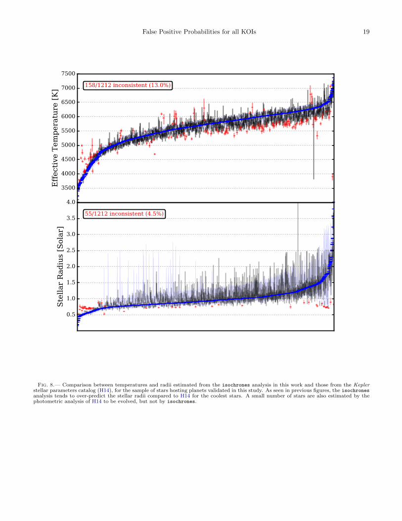
While the FPP below which to claim planet validationis clearly an arbitrary choice, there is precedent to usingFPP < 0.01 as the threshold—Rowe et al. (2014) vali-dated over 800 multi-planet KOIs using this number, andMontet et al. (2015) used it to validate a sample of K2-Campaign 1 planets. Adopting this same threshold andadding the 0.06% residual FPP estimated in Section 4.3to the vespa-calculated value, we find that of the KOIswith reliable vespa FPPs, 1935 have FPP < 0.01, andare thus validated at the 99% level. These KOIs arelabeled as such in Table 6. These are not all new val-idations, however, since a number of them are alreadyCONFIRMED. FIG. 6 shows a different kind of sum-mary, grouping KOIs by disposition and splitting up theCANDIDATES according to the vespa results, showingthat 1284 KOIs are newly validated at the 99% level.FIG. 7 shows the radii and periods of the CONFIRMEDand CANDIDATE KOIs, with the transparency of thepoints representing the vespa-calculated FPP. FIG. 8compares the temperature and radii of the stars hostingthese planets between the H14 and isochrones analysis.

As there is significant interest in identifying potentiallyhabitable planets, Table 3 lists the properties of 9 CAN-DIDATE KOIs newly validated by this work that may

fall within the optimistic habitable zones of their hoststars (Kopparapu et al. 2013), according to the stellarproperties reported by the DR24 table at the NExScIArchive. We note that while more detailed follow-up ob-servations (imaging and spectroscopy) have been takenfor each of these targets, we make no attempt here tocharacterize these systems in detail. However, we do notethat high-resolution imaging of KOI-2418 and KOI-3010reveal that these two host stars have close companionsthat may or may not change the habitable nature of theplanets (e.g., if the planets happen to transit the sec-ondary star instead of the primary). Additionally, anal-ysis of high-resolution spectroscopy will solidify the prop-erties of all these host stars, affecting the habitable zoneboundaries. We thus emphasize that this list is neithercomplete nor final, serving only to draw attention to newvalidations of interest rather than to be a definitive state-ment on potential habitability. We also note that basedsolely on the properties in the DR24 table, KOI-5475.01(listed as having a 448-day orbital period) should also beincluded in this list of potentially habitable-zone planets.However, as explained in Coughlin et al. (2015b, Section5.5.4), this particular KOI actually has a 224-day period,making its insolation too high to be within the habitablezone; we have thus excluded it from Table 3.

4.5. Likely False Positives

In addition to the confident validations, we identify 428KOIs that currently have CANDIDATE disposition butfor which vespa calculates FPP > 0.9; these KOIs arelikely to be false positives. As FIG. 7 shows, many ofthese newly identified false positives have large radii—this is again because of the dispositioning philosophyadopted by the Kepler team, which does not use anycut in transit depth or inferred “planet” size to iden-tify FALSE POSITIVES. To identify these likely falsepositives from the vespa calculations, we do not requireCANDIDATES to obey the same selections we used toensure a clean sample for validation. This is because evenif a signal has characteristics such that a low vespa FPPwould not be sufficient to validate it, a high vespa FPPis still sufficient to cast doubt on its planetary nature.As a demonstration of the ability of vespa to identifyfalse positives, FIG. 5 shows the FPPs for KOIs that aredispositioned FALSE POSITIVE and have MES > 10.The vast majority of these have large FPPs.

One final note about these calculations is that uniden-tified transit timing variations (TTVs) will increase theFPP of a transit signal, as the shape of the folded lightcurve will be distorted, typically resulting in a longer sig-nal which a trapezoid model will also identify as more V-shaped. While we have analyzed light curves correctingfor known TTVs when available, we have also undoubt-edly missed many systems with as-yet-unspecified TTVsignals. This means that a large FPP may be simplyan indication of unidentified TTVs rather than an astro-physical false positive, especially in multi-planet systems,which should overall have a very low false positive rate(Lissauer et al. 2014; Rowe et al. 2014). It is thus prob-able that despite multi-KOIs having lower FPPs thansingles (Table 2), even these relatively low FPPs are in-flated by the effect of TTVs. Table 6 lists whether knownTTVs were accounted for when constructing the foldedtransit light curve for each KOI.

False Positive Probabilities for all KOIs 7

TABLE 3Newly Validated Planets in the Optimistic Habitable Zone.

KOI Kepler name Period RP Fp Teff log g R? M?

[days] R⊕ Fe [K] R� M�

463.01 Kepler-560 b 18.478 1.57+0.26−0.26 1.26+0.58

−0.43 3387+59−50 4.96+0.10

−0.10 0.30+0.05−0.05 0.30+0.05

−0.05

854.01 Kepler-705 b 56.056 1.96+0.25−0.25 0.64+0.23

−0.18 3593+58−66 4.78+0.08

−0.08 0.47+0.06−0.06 0.49+0.06

−0.06

2418.01 Kepler-1229 b 86.829 1.12+0.13−0.22 0.35+0.12

−0.14 3724+60−74 4.84+0.09

−0.08 0.41+0.05−0.08 0.43+0.05

−0.07

3010.01 Kepler-1410 b 60.866 1.56+0.15−0.15 0.93+0.25

−0.21 3903+50−60 4.74+0.06

−0.06 0.52+0.05−0.05 0.54+0.05

−0.05

3282.01 Kepler-1455 b 49.277 1.97+0.25−0.19 1.30+0.50

−0.34 3894+83−101 4.71+0.06

−0.07 0.54+0.07−0.05 0.55+0.06

−0.06

4036.01 Kepler-1544 b 168.811 1.83+4.73−0.17 1.02+13.70

−0.25 4893+141−110 4.54+0.06

−0.98 0.76+1.97−0.07 0.73+0.28

−0.06

4356.01 Kepler-1593 b 174.510 1.91+0.16−0.21 0.29+0.09

−0.09 4366+131−166 4.82+0.06

−0.05 0.46+0.04−0.05 0.49+0.03

−0.05

4450.01 Kepler-1606 b 196.435 1.98+0.72−0.15 1.38+1.48

−0.32 5536+161−140 4.57+0.03

−0.24 0.82+0.29−0.06 0.90+0.09

−0.09

5856.01 Kepler-1638 b 259.337 1.70+0.76−0.21 1.47+2.03

−0.44 5906+183−147 4.47+0.10

−0.29 0.85+0.38−0.10 0.77+0.10

−0.04

Note. — This table lists CANDIDATE KOIs validated in this work that may lie within the optimistichabitable zones of their host stars. The stellar and planetary properties for this table are taken fromthe DR24 table at the NExScI Exoplanet Archive. Further individual study of each of these systemsusing detailed follow-up observations will either solidify or amend their potentially habitable nature.In particular, we note that high-resolution imaging observations on the CFOP archivea reveal bothKOI-2418 and KOI-3010 to have close companions which may or may not affect their habitable nature.

ahttp://cfop.ipac.caltech.edu

4.6. Blended Transiting Planets?

In this work, the only astrophysical false positive sce-narios we consider are eclisping binary stars (EB, HEB,BEB, and the double-period versions thereof). Previouswork studying Kepler false positive rates (e.g. Fressinet al. 2013) has also considered the “blended transitingplanet” to be a false positive—i.e., a fainter companionstar hosting a transiting planet larger than what wouldbe inferred if it were transiting the target star. Becausewe do not consider such a scenario to be a false positive,the vespa analysis presented here does not quantify itsprobability. As a result, we are not able to unambigu-ously determine the radii of the planets we validate— allthe planet radii listed in Table 6 are based on the assump-tion that the planet transits the target star and that thetarget star is unblended. If the target star is actually amember of an unresolved binary system (as a significantfraction of KOIs undoubtedly are), then the true planetradius will be larger (significantly larger if transiting afainter companion). This was indeed the motivation forFressin et al. (2013) to consider the “blended transitingplanet” as a false positive; part of the goal of that workwas to compute the planet occurrence rates in differentradius bins. However, trying to distinguish between sin-gle and binary target star configurations is beyond thescope of this work; we thus follow the precedent of Lis-sauer et al. (2014, especially Section 5) by acknowledgingthe potential for substantial radius uncertainties amongthe validated planet sample while nevertheless defendingthe validations themselves as robust.

4.7. Failure Modes

We were not able to successfully run vespa on all of theKOIs. The various reasons for these occasional failuresare detailed below.

1. 28 KOIs did not receive MCMC modeling. Mostof these have been are already designated FALSEPOSITIVE at the archive.

2. 233 KOIs did receive MCMC modeling but had un-physical fit results; e.g., negative Rp/R? or best-fit

impact parameter greater than (1+Rp/R?). TheseKOIs were left out of the vespa calculations.

3. The host stars of 74 KOIs are not included in theH14 stellar property catalog, and thus were not in-cluded in this analysis.

4. 8 KOIs have no koi_depth_err1 value on thearchive, and thus had no weak secondary constraintand were left out of the calculations.

5. For 38 KOIs, the trapezoid MCMC fit did not con-verge. The convergence criterion was for the auto-correlation time of the chain for each parameter tobe shorter than 10% of the total chain length.

6. For 39 KOIs, the orbital period and stellar proper-ties of the candidate imply the orbit to be withinits host star’s Roche limit. This usually happenswhen the host star is estimated to be a giant, andthese situations are nearly always false positives.

The numbers in this list correspond to the numbers inthe “failure” column in Table 6.

5. COMPARISON WITH FOLLOW-UP OBSERVATIONALSTUDIES

One of the difficulties with probabilistic validation isthat, by necessity, it is typically invoked when no othermethod of follow-up confirmation is possible. It cantherefore be difficult to find ways to compare the re-sults of a calculation such as vespa to any known obser-vational ground-truth, or to “validate the validations.”However, because so much follow-up observational efforthas gone into Kepler candidates over the last few years,there actually are two different datasets that do providesuch information for relatively small subsets of candi-dates. Here, we discuss the results of vespa calculationsfor these candidates and the impliciations for the relia-bility of the vespa framework.

5.1. Spitzer photometry

8 Morton et al.

The first of these datasets is from Desert et al. (2015),who observe the transits of 50 Kepler candidates withthe Spitzer Space Telescope in order to observationallyconstrain the FP rate. The idea behind these observa-tions is that a blended EB false positive will often showa color-dependent transit depth, and so comparing thecandidate depths measured by Kepler to those measuredin the infrared by Spitzer would give an idea of how likelya signal is to be a false positive. The results of their anal-ysis suggest that fewer than 8% of their observed candi-dates are likely to be false positives. Of these 50 candi-dates, vespa on its own calculates FPP > 0.1 for four.Two of these (KOI-103.01 and KOI-248.02) are systemswith known significant TTVs; the other two (KOI-247.01and KOI-555.02) are likely false positives, with FPPs of0.90 and 0.81, respectively. For all but two of the re-maining candidates, vespa gives FPP < 0.01. The falsepositive rates calculated in Desert et al. (2015) are alsobased on probabilistic arguments very similar to Mor-ton & Johnson (2011) and thus are not quite candidatesfor “ground-truth” comparison, but the lack of transitchromaticity and the agreements between these two in-dependent studies are certainly supportive of the vesparesults.

5.2. Radial-velocity monitoring of large candidates

A much more independent and powerful test data sethas recently become available in the work of Santerneet al. (2015), which presented the results of a long-termRV-monitoring campaign targeting 129 Kepler giant-planet candidates. Of these, they confirm 45 to be plan-ets and identify 48 as eclipsing binaries, 15 as contam-inating EBs (CEBs), and 3 as brown dwarfs. They areunable to determine the nature of the remaining 18.These results imply a relatively high FP rate amonggiant-planet candidates, possibly near 50%, which soundspotentially concerning, although we reiterate that KOIsare not ruled FALSE POSITIVES based on their transitdepth or inferred size alone. Additionally, when we lookat the vespa results on this sample, we see very goodagreement between our results and the RV- detected“ground truth” (Table 4). Notably, confirmed planetsshow a mean FPP of about 10% and a median of muchless than 1%, while confirmed EBs (CEBs) show a meanFPP of 75% (78%) and a median of 97% (99%). Thethree brown dwarfs also show low FPPs, which is under-standable because vespa doesn’t pretend to predict any-thing about the mass of the companion, and BDs are es-sentially the same size as giant planets. It is also instruc-tive to investigate the four cases where vespa computeshigh FPPs (>0.5) for confirmed planets. Three of these(KOI-377.01, KOI-1426.02 and KOI-1474.01) have signif-icant TTVs, and one is a grazing eclipse (KOI-614.01).KOI-1474.01 is also on a highly eccentric orbit (Dawsonet al. 2012), in addition to its TTVs, which also con-tributes to its high FPP. Overall, this comparison pow-erfully demonstrates the reliability of the vespa calcu-lation, showing that even in a population of candidatesthat include many false positives, it is able to effectivelyidentify which are true planets and which are not.

5.3. The enigmatic case of KOI-6705.01

We also briefly discuss another case of individual inter-est. KOI-6705.01, a 0.99 d signal around a mid M-dwarf

TABLE 4vespa–calculated FPPs of theSanterne (2015) RV sample

RV-based nature Number mean FPP median FPP

Planet 43 0.1 3.6e-05Brown dwarf 3 0.012 0.0026

Eclipsing binary (EB) 43 0.75 0.97Contaminating EB 13 0.78 0.99

Undetermined 18 0.31 0.01

star, was identified as a KOI of possible interest by Gai-dos et al. (2015). After significant follow-up observationsand detailed full-frame image analysis, they concludedthat the signal was most likely due to a charge-transfereffect from a 1.99 d EB located on the same CCD col-umn. For this KOI, vespa calculates an FPP of 1, withthe “long” model preferred by far (of the astrophysicalmodels, the double-period BEB—the true scenario—ispreferred). This is an excellent example of what wasdiscussed in Section 4.3: that even effects like columnanomalies that were not identified by the Kepler teamas ephemeris matches will typically be identified as falsepositives by vespa.

6. CONCLUSIONS

In this work, we have calculated the astrophysical falsepositive probability (FPP) for every Kepler object of in-terest (KOI) in the Q1-Q17 DR24 table, using the pub-licly available Python module vespa, which implementsthe procedure introduced in Morton (2012), with im-provements in stellar parameter modeling and the inclu-sion of new “double-period” false positive scenarios andartificial models to identify KOIs that are not well ex-plained by any of the astrophysical models. We have alsofor the first time estimated uncertainties in the vespacalculation, through a bootstrap resampling procedure.

While the assumptions behind this calculation are notnecessarily valid for every KOI (see Section 4.2), we haveidentified 1284 KOIs that have reliable FPPs of < 0.01,resulting in validation of their planetary nature at the99% confidence level, more than doubling the number ofconfirmed Kepler exoplanets. Among this set of newlyvalidated planets are 9 that are consistent with being inthe habitable zones of their host stars. We also identify428 new likely false positive KOIs, although we note thatsome of these may be due to unidentified or miscorrectedtransit timing variations.

The reliability of these calculations depends signifi-cantly on the results of Bryson & Morton (2015), whichquantify the probability that the eclipse/transit signal isspatially coincident on the sky with the presumed tar-get star. Without confirmation that the transit signalis not coming from a significantly displaced source, thesky area used as part of the prior for the false positivescenarios would need to be significantly larger than thepositional uncertainty value assumed in this work (de-scribed in Section 2.1). Additionally, the blended falsepositive scenarios vespa considers are assumed to be fullycontained within the photometric aperture; this assump-tion would also be broken if the source of the eclipse weresignificantly displaced. We estimate that perhaps 0.06%of the planets we validate could be signals coming fromsignificantly displaced sources, similar to those identified

False Positive Probabilities for all KOIs 9

as period-epoch matches by Coughlin et al. (2014) butunidentified by that analysis.

While previous a priori false positive rate estimates(Morton & Johnson 2011; Fressin et al. 2013) have madeclear that the Kepler planet candidate catalogs are gen-erally low enough to ignore for the purposes of planetoccurrence rate calculations, any more detailed study ofany small subset of individual KOIs should understand inmore detail the FPPs of those specific candidates. Thistype of small-sample candidate culling using individuallycalculated FPPs has already been done in the literature(Morton & Swift 2014; Morton & Winn 2014); the pub-lication of this full catalog allows the community to dothe same. In particular, several other studies have shownthat specific samples of KOIs tend to have larger FPPsthan the global average, so studies involving giant-planetKOIs (Santerne et al. 2015) or evolved stars (Sliski &Kipping 2014) are in even greater need of the individualFPP analysis here presented.

The Kepler mission has demonstrated that space-based transiting planet surveys identify planet candi-dates at a rate much faster than traditional follow-uptechniques can confirm them. As a result, false posi-tive probability quantification techniques are now an in-tegral part of the landscape of exoplanet science. Whilethe present work is the first large-scale demonstrationof a fully automated validation procedure, there is muchprogress still to be made. For example, there is currentlyno support within vespa to calculate the FPP for a can-didate which has a specifically identified but previouslyunknown close companion. Future development plans forthe vespa package include support for this scenario, aswell as other improvements. One of the most importantof these will be to allow for a contaminating EB to not befully contained within the target photometric aperture;that is, modeling the probability for further-away starsto be EBs contributing only a small amount of their fluxto the target photometry, such as is the case for manyof the false positives identified via ephemeris matchingby Coughlin et al. (2014). Full inclusion of this effectwill allow for even low-SNR candidates to receive confi-dent vespa analysis, which is now limited only to KOIsfor which confident pixel-level positional analysis is pos-sible.

Beyond Kepler, future transit missions such as TESSand PLATO will require automated false positive analy-sis in order to efficiently sift through the large numbers ofcandidates that they will find. This work demonstratesthat vespa will be a valuable tool towards this purpose.

Instructions for reproducing all the calculations pre-sented herein can be found at https://github.com/timothydmorton/koi-fpp. Summary figures producedby vespa for all KOIs can be accessed at http://kepler-fpp.space.

TDM acknowledges support from the Kepler Partici-pating Scientist Program (NNX14AE11G). We thank theanonymous referee, Daniel Huber, Jack Lissauer, JunaKollmeier, and David Hogg for providing helpful sugges-tions that improved both the analysis and presentationherein. This paper includes data collected by the Ke-pler mission. Funding for the Kepler mission is provided

by the NASA Science Mission directorate. The authorsacknowledge the efforts of the Kepler Mission team forobtaining the light curve products used in this publica-tion, which were generated by the Kepler Mission sciencepipeline through the efforts of the Kepler Science Oper-ations Center and Science Office. The Kepler Mission isled by the project office at NASA Ames Research Center.Ball Aerospace built the Kepler photometer and space-craft which is operated by the mission operations centerat LASP. These data products are archived at the NASAExoplanet Science Institute, which is operated by theCalifornia Institute of Technology, under contract withthe National Aeronautics and Space Administration un-der the Exoplanet Exploration Program. This researchhas made use of NASA’s Astrophysics Data System.

10 Morton et al.

REFERENCES

Bastien, F. A., Stassun, K. G., & Pepper, J. 2014, ApJ, 788, L9Becker, J. C., Vanderburg, A., Adams, F. C., Rappaport, S. A., &

Schwengeler, H. M. 2015, ApJ, 812, L18Borucki, W. J., Koch, D. G., Batalha, N., et al. 2012, ApJ, 745,

120Bryson, S. T., & Morton, T. D. 2015, KSCI-19092-001Bryson, S. T., Jenkins, J. M., Gilliland, R. L., et al. 2013, PASP,

125, 889Buchner, J., Georgakakis, A., Nandra, K., et al. 2014, A&A, 564,

A125Burke, C. J., Christiansen, J. L., Mullally, F., et al. 2015, ApJ,

809, 8Casagrande, L., Schonrich, R., Asplund, M., et al. 2011, A&A,

530, A138Coughlin, J. L., Thompson, S. E., Bryson, S. T., et al. 2014, AJ,

147, 119Coughlin, J. L., Bryson, S. T., Burke, C. J., et al. 2015a,

KSCI-19104-001Coughlin, J. L., Mullally, F., Thompson, S. E., et al. 2015b,

ArXiv e-prints, arXiv:1512.06149Dawson, R. I., Johnson, J. A., Morton, T. D., et al. 2012, ApJ,

761, 163Delfosse, X., Forveille, T., Segransan, D., et al. 2000, A&A, 364,

217Desert, J.-M., Charbonneau, D., Torres, G., et al. 2015, ApJ, 804,

59Dıaz, R. F., Almenara, J. M., Santerne, A., et al. 2014, MNRAS,

441, 983Dotter, A., Chaboyer, B., Jevremovic, D., et al. 2008, ApJS, 178,

89Dressing, C. D., & Charbonneau, D. 2013, ApJ, 767, 95Fabrycky, D. C., Ford, E. B., Steffen, J. H., et al. 2012, ApJ, 750,

114Feiden, G. A., Chaboyer, B., & Dotter, A. 2011, ApJ, 740, L25Feroz, F., Hobson, M. P., & Bridges, M. 2009, MNRAS, 398, 1601—. 2011, MultiNest: Efficient and Robust Bayesian Inference,

Astrophysics Source Code Library, ascl:1109.006Feroz, F., Hobson, M. P., Cameron, E., & Pettitt, A. N. 2013,

ArXiv e-printsFord, E. B., Fabrycky, D. C., Steffen, J. H., et al. 2012, ApJ, 750,

113Foreman-Mackey, D., Hogg, D. W., Lang, D., & Goodman, J.

2013, PASP, 125, 306Foreman-Mackey, D., Hogg, D. W., & Morton, T. D. 2014, ApJ,

795, 64Fressin, F., Torres, G., Charbonneau, D., et al. 2013, ApJ, 766, 81Gaidos, E., Mann, A. W., & Ansdell, M. 2015, ArXiv e-prints,

arXiv:1511.06471Hayden, M. R., Bovy, J., Holtzman, J. A., et al. 2015, ArXiv

e-prints

Huber, D., Silva Aguirre, V., Matthews, J. M., et al. 2014, ApJS,211, 2

Jontof-Hutter, D., Ford, E. B., Rowe, J. F., et al. 2015, ArXive-prints, arXiv:1512.02003

Kipping, D. M., Torres, G., Buchhave, L. A., et al. 2014, ApJ,795, 25

Kopparapu, R. K., Ramirez, R., Kasting, J. F., et al. 2013, ApJ,765, 131

Lissauer, J. J., Marcy, G. W., Rowe, J. F., et al. 2012, ApJ, 750,112

Lissauer, J. J., Marcy, G. W., Bryson, S. T., et al. 2014, ApJ,784, 44

Marcy, G. W., Isaacson, H., Howard, A. W., et al. 2014, ApJS,210, 20

Montet, B. T., Morton, T. D., Foreman-Mackey, D., et al. 2015,ArXiv e-prints

Morton, T. 2014, PhD thesis, California Institute of TechnologyMorton, T. D. 2012, ApJ, 761, 6—. 2015a, isochrones: Stellar model grid package, Astrophysics

Source Code Library, ascl:1503.010—. 2015b, VESPA: False positive probabilities calculator,

Astrophysics Source Code Library, ascl:1503.011Morton, T. D., & Johnson, J. A. 2011, ApJ, 738, 170Morton, T. D., & Swift, J. 2014, ApJ, 791, 10Morton, T. D., & Winn, J. N. 2014, ApJ, 796, 47

Moutou, C., Almenara, J. M., Dıaz, R. F., et al. 2014, MNRAS,444, 2783

Muirhead, P. S., Johnson, J. A., Apps, K., et al. 2012, ApJ, 747,144

Petigura, E. A., Howard, A. W., & Marcy, G. W. 2013,Proceedings of the National Academy of Science, 110, 19273

Pinsonneault, M. H., An, D., Molenda-Zakowicz, J., et al. 2012,ApJS, 199, 30

Rowe, J. F., Bryson, S. T., Marcy, G. W., et al. 2014, ApJ, 784,45

Rowe, J. F., Coughlin, J. L., Antoci, V., et al. 2015, ApJS, 217, 16Santerne, A., Dıaz, R. F., Moutou, C., et al. 2012, A&A, 545, A76Santerne, A., Hebrard, G., Deleuil, M., et al. 2014, A&A, 571,

A37Santerne, A., Moutou, C., Tsantaki, M., et al. 2015, ArXiv

e-prints, arXiv:1511.00643Schlegel, D. J., Finkbeiner, D. P., & Davis, M. 1998, ApJ, 500,

525Sliski, D. H., & Kipping, D. M. 2014, ApJ, 788, 148Steffen, J. H., Fabrycky, D. C., Ford, E. B., et al. 2012, MNRAS,

421, 2342Steffen, J. H., Fabrycky, D. C., Agol, E., et al. 2013, MNRAS,

428, 1077Swift, J. J., Johnson, J. A., Morton, T. D., et al. 2013, ApJ, 764,

105Torres, G., Kipping, D. M., Fressin, F., et al. 2015, ApJ, 800, 99

False Positive Probabilities for all KOIs 11

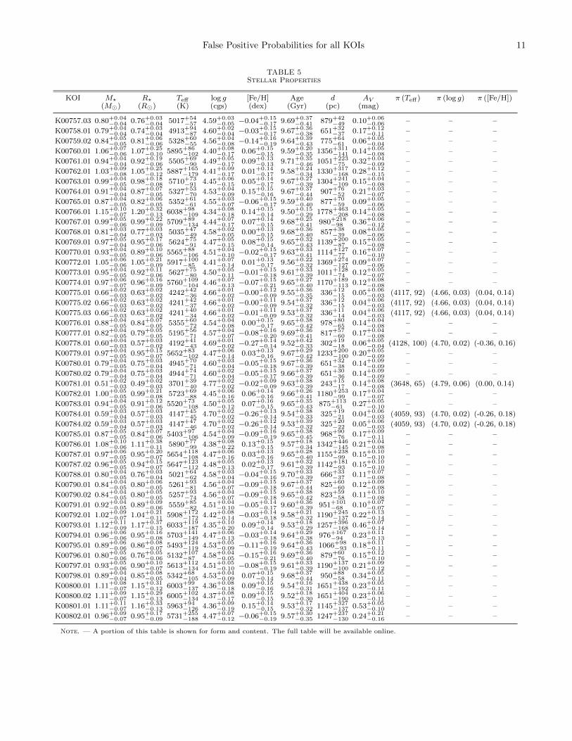
TABLE 5Stellar Properties

KOI M? R? Teff log g [Fe/H] Age d AV π (Teff) π (log g) π ([Fe/H])(M�) (R�) (K) (cgs) (dex) (Gyr) (pc) (mag)

K00757.03 0.80+0.04−0.04 0.76+0.03

−0.04 5017+54−57 4.59+0.03

−0.05 −0.04+0.15−0.17 9.69+0.37

−0.41 879+42−49 0.10+0.06

−0.06 – – –

K00758.01 0.79+0.04−0.04 0.74+0.03

−0.04 4913+94−87 4.60+0.02

−0.04 −0.03+0.15−0.17 9.67+0.36

−0.38 651+32−37 0.17+0.12

−0.11 – – –

K00759.02 0.84+0.05−0.05 0.81+0.06

−0.06 5328+60−55 4.56+0.04

−0.08 −0.14+0.16−0.19 9.64+0.39

−0.43 775+64−61 0.06+0.05

−0.04 – – –

K00760.01 1.06+0.07−0.06 1.07+0.25

−0.10 5895+86−102 4.40+0.08

−0.17 0.06+0.15−0.15 9.59+0.20

−0.35 1356+311−141 0.14+0.05

−0.08 – – –

K00761.01 0.94+0.04−0.04 0.92+0.19

−0.06 5505+69−90 4.49+0.05

−0.17 0.09+0.13−0.13 9.71+0.35

−0.46 1051+223−75 0.32+0.04

−0.09 – – –

K00762.01 1.03+0.09−0.08 1.05+0.25

−0.12 5887+165−179 4.41+0.09

−0.17 0.01+0.14−0.17 9.58+0.24

−0.34 1330+317−168 0.28+0.12

−0.15 – – –

K00763.01 0.99+0.04−0.05 0.98+0.18

−0.08 5710+73−91 4.45+0.06

−0.15 0.05+0.14−0.17 9.67+0.27

−0.39 1304+241−109 0.15+0.04

−0.08 – – –

K00764.01 0.91+0.04−0.04 0.87+0.07

−0.05 5327+53−70 4.53+0.04

−0.09 0.15+0.15−0.16 9.67+0.37

−0.44 907+76−52 0.21+0.03

−0.07 – – –

K00765.01 0.87+0.04−0.05 0.82+0.06

−0.05 5352+61−61 4.55+0.03

−0.07 −0.06+0.15−0.17 9.59+0.40

−0.40 877+70−59 0.09+0.05

−0.06 – – –

K00766.01 1.15+0.10−0.07 1.20+0.32

−0.13 6038+98−109 4.34+0.08

−0.18 0.14+0.15−0.14 9.50+0.15

−0.29 1778+463−208 0.14+0.05

−0.08 – – –

K00767.01 0.99+0.05−0.06 0.99+0.22

−0.09 5709+89−134 4.44+0.07

−0.17 0.07+0.14−0.15 9.68+0.25

−0.41 980+218−98 0.36+0.06

−0.12 – – –

K00768.01 0.81+0.03−0.04 0.77+0.03

−0.03 5035+47−49 4.58+0.02

−0.05 0.00+0.13−0.15 9.68+0.36

−0.40 857+38−39 0.08+0.05

−0.06 – – –

K00769.01 0.97+0.05−0.04 0.95+0.17

−0.06 5624+75−91 4.47+0.05

−0.15 0.08+0.15−0.14 9.65+0.32

−0.43 1139+200−87 0.15+0.05

−0.08 – – –

K00770.01 0.93+0.04−0.05 0.89+0.10

−0.06 5565+88−106 4.51+0.04

−0.10 −0.02+0.15−0.17 9.63+0.33

−0.41 1114+127−77 0.16+0.07

−0.10 – – –

K00772.01 1.05+0.06−0.06 1.05+0.21

−0.09 5917+100−85 4.41+0.07

−0.14 0.01+0.13−0.17 9.56+0.22

−0.32 1369+274−127 0.09+0.07

−0.06 – – –

K00773.01 0.95+0.04−0.05 0.92+0.11

−0.06 5627+75−80 4.50+0.05

−0.11 −0.01+0.15−0.18 9.61+0.33

−0.39 1011+128−74 0.12+0.05

−0.07 – – –

K00774.01 0.97+0.06−0.07 0.96+0.16

−0.09 5760+109−104 4.46+0.07

−0.13 −0.07+0.15−0.21 9.65+0.27

−0.40 1170+189−113 0.12+0.08

−0.08 – – –

K00775.01 0.66+0.02−0.03 0.63+0.02

−0.02 4242+42−36 4.66+0.01

−0.02 −0.00+0.12−0.09 9.55+0.36

−0.35 336+12−15 0.05+0.06

−0.03 (4117, 92) (4.66, 0.03) (0.04, 0.14)

K00775.02 0.66+0.02−0.03 0.63+0.02

−0.02 4241+42−37 4.66+0.01

−0.02 −0.00+0.11−0.09 9.54+0.37

−0.32 336+12−15 0.04+0.06

−0.03 (4117, 92) (4.66, 0.03) (0.04, 0.14)

K00775.03 0.66+0.02−0.03 0.63+0.02

−0.02 4241+40−34 4.66+0.01

−0.02 −0.01+0.11−0.09 9.53+0.37

−0.32 336+11−14 0.04+0.06

−0.03 (4117, 92) (4.66, 0.03) (0.04, 0.14)

K00776.01 0.88+0.04−0.05 0.84+0.07

−0.05 5355+60−72 4.54+0.04

−0.08 0.00+0.15−0.17 9.65+0.38

−0.42 978+80−65 0.14+0.04

−0.08 – – –

K00777.01 0.82+0.04−0.05 0.79+0.05

−0.05 5195+56−71 4.57+0.04

−0.07 −0.08+0.16−0.20 9.69+0.36

−0.41 817+57−60 0.17+0.04

−0.08 – – –

K00778.01 0.60+0.04−0.03 0.57+0.03

−0.02 4192+41−43 4.69+0.01

−0.02 −0.27+0.14−0.14 9.52+0.42

−0.33 302+19−18 0.06+0.05

−0.04 (4128, 100) (4.70, 0.02) (-0.36, 0.16)

K00779.01 0.97+0.04−0.05 0.95+0.15

−0.07 5652+83−102 4.47+0.06

−0.14 0.03+0.13−0.16 9.67+0.29

−0.42 1233+200−100 0.20+0.05

−0.09 – – –

K00780.01 0.79+0.04−0.05 0.75+0.03

−0.04 4945+70−71 4.60+0.03

−0.04 −0.05+0.15−0.18 9.67+0.36

−0.39 651+32−38 0.14+0.09

−0.09 – – –

K00780.02 0.79+0.04−0.04 0.75+0.03

−0.04 4944+74−71 4.60+0.02

−0.04 −0.05+0.15−0.17 9.66+0.37

−0.39 651+30−36 0.14+0.09

−0.09 – – –

K00781.01 0.51+0.02−0.03 0.49+0.02

−0.03 3701+39−40 4.77+0.02

−0.02 −0.02+0.09−0.09 9.63+0.38

−0.39 243+15−17 0.14+0.08

−0.08 (3648, 65) (4.79, 0.06) (0.00, 0.14)

K00782.01 1.00+0.05−0.05 0.99+0.21

−0.08 5723+69−88 4.45+0.06

−0.16 0.06+0.14−0.16 9.66+0.26

−0.41 1180+253−99 0.17+0.04

−0.07 – – –

K00783.01 0.94+0.04−0.05 0.91+0.12

−0.06 5520+73−108 4.50+0.05

−0.12 0.07+0.16−0.15 9.65+0.35

−0.43 875+113−61 0.27+0.05

−0.10 – – –

K00784.01 0.59+0.03−0.04 0.57+0.03

−0.03 4147+45−45 4.70+0.02

−0.02 −0.26+0.13−0.14 9.54+0.38

−0.33 325+19−21 0.04+0.06

−0.03 (4059, 93) (4.70, 0.02) (-0.26, 0.18)

K00784.02 0.59+0.03−0.04 0.57+0.03

−0.03 4147+47−46 4.70+0.02

−0.02 −0.26+0.12−0.14 9.53+0.39

−0.32 325+20−22 0.05+0.06

−0.03 (4059, 93) (4.70, 0.02) (-0.26, 0.18)

K00785.01 0.87+0.05−0.05 0.84+0.07

−0.06 5403+97−106 4.54+0.04

−0.09 −0.09+0.16−0.19 9.65+0.38

−0.45 968+90−76 0.17+0.09

−0.11 – – –

K00786.01 1.08+0.10−0.06 1.11+0.38

−0.11 5890+77−99 4.38+0.08

−0.22 0.13+0.15−0.15 9.57+0.18

−0.34 1342+446−145 0.21+0.04

−0.08 – – –

K00787.01 0.97+0.06−0.05 0.95+0.20

−0.07 5654+118−108 4.47+0.06

−0.16 0.03+0.13−0.16 9.65+0.28

−0.40 1155+238−99 0.15+0.10

−0.10 – – –

K00787.02 0.96+0.05−0.05 0.94+0.15

−0.07 5647+123−112 4.48+0.05

−0.13 0.02+0.13−0.17 9.61+0.32

−0.39 1142+181−93 0.15+0.10

−0.10 – – –

K00788.01 0.80+0.04−0.05 0.76+0.03

−0.04 5021+64−62 4.58+0.03

−0.04 −0.04+0.15−0.16 9.70+0.33

−0.39 666+33−37 0.11+0.07

−0.08 – – –

K00790.01 0.84+0.04−0.05 0.80+0.06

−0.05 5261+93−81 4.56+0.04

−0.07 −0.09+0.15−0.18 9.67+0.37

−0.44 825+60−60 0.12+0.09

−0.08 – – –

K00790.02 0.84+0.04−0.05 0.80+0.05

−0.05 5257+93−74 4.56+0.04

−0.07 −0.09+0.15−0.18 9.65+0.38

−0.42 823+59−58 0.11+0.10

−0.08 – – –

K00791.01 0.92+0.04−0.05 0.89+0.09

−0.06 5559+85−82 4.51+0.04

−0.10 −0.05+0.14−0.17 9.60+0.36

−0.39 951+101−68 0.10+0.07

−0.07 – – –

K00792.01 1.02+0.09−0.07 1.04+0.21

−0.11 5908+172−172 4.42+0.08

−0.14 −0.03+0.14−0.18 9.58+0.21

−0.32 1190+245−137 0.22+0.13

−0.14 – – –

K00793.01 1.12+0.11−0.09 1.17+0.37

−0.15 6033+119−187 4.35+0.10

−0.20 0.09+0.14−0.14 9.53+0.18

−0.29 1257+396−168 0.46+0.07

−0.14 – – –

K00794.01 0.96+0.06−0.06 0.95+0.16

−0.08 5703+141−149 4.47+0.06

−0.13 −0.03+0.14−0.18 9.64+0.29

−0.38 976+167−94 0.23+0.11

−0.13 – – –

K00795.01 0.89+0.06−0.06 0.86+0.08

−0.07 5493+124−119 4.53+0.05

−0.09 −0.11+0.16−0.19 9.64+0.36

−0.43 1066+98−93 0.18+0.11

−0.11 – – –

K00796.01 0.80+0.05−0.06 0.76+0.05

−0.06 5132+107−87 4.58+0.04

−0.05 −0.15+0.16−0.21 9.69+0.36

−0.40 879+60−76 0.15+0.12

−0.10 – – –

K00797.01 0.93+0.05−0.06 0.90+0.10

−0.07 5613+112−134 4.51+0.05

−0.10 −0.08+0.15−0.19 9.61+0.33

−0.39 1190+137−100 0.21+0.09

−0.12 – – –

K00798.01 0.89+0.04−0.04 0.85+0.08

−0.05 5342+68−105 4.53+0.04

−0.09 0.07+0.15−0.14 9.68+0.37

−0.44 950+88−58 0.34+0.05

−0.11 – – –

K00800.01 1.11+0.08−0.07 1.15+0.31

−0.12 6003+99−137 4.36+0.08

−0.18 0.09+0.15−0.16 9.54+0.16

−0.31 1651+438−192 0.23+0.05

−0.11 – – –

K00800.02 1.11+0.09−0.07 1.15+0.29

−0.13 6005+102−134 4.37+0.08

−0.17 0.09+0.15−0.15 9.52+0.18

−0.30 1651+404−190 0.23+0.06

−0.11 – – –

K00801.01 1.11+0.11−0.07 1.16+0.33

−0.13 5963+94−126 4.36+0.09

−0.19 0.15+0.14−0.15 9.53+0.17

−0.32 1145+327−137 0.53+0.05

−0.10 – – –

K00802.01 0.96+0.09−0.07 0.95+0.17

−0.09 5731+255−188 4.47+0.07

−0.12 −0.06+0.15−0.19 9.57+0.30

−0.35 1247+237−130 0.24+0.21

−0.16 – – –

Note. — A portion of this table is shown for form and content. The full table will be available online.

12 Morton et al.

7000

8000

9000

10000

11000

12000

Eff

ect

ive T

em

pera

ture

[K

] 135/563 inconsistent (24.0%)

4500

5000

5500

6000

6500

7000

Eff

ect

ive T

em

pera

ture

[K

] 825/5165 inconsistent (16.0%)

2500

3000

3500

4000

4500

5000

Eff

ect

ive T

em

pera

ture

[K

] 133/374 inconsistent (35.6%)

Fig. 1.— Comparison between effective temperatures estimated from the isochrones analysis in this work and those from the Keplerstellar parameters catalog (Huber et al. 2014, hereafter H14). Bottom panel shows stars for which H14 predicts Teff < 4500 K, middle spans4500 K < Teff < 6500 K, and top has Teff > 6500 K. Blue horizontal bold lines are the H14 values in sorted order; blue shading representsthe error bars from H14. Vertical lines span the 1σ credible region of the isochrones fits; these lines are grey if they overlap with theH14 1σ region and red (with the median marked by a point) if they are inconsistent. This comparison shows that the stellar parametersestimated in this work are broadly consistent with H14, though less so for the coolest and hottest stars.

False Positive Probabilities for all KOIs 13

2.5

2.0

1.5

1.0

0.5

0.0

0.5

1.0

[Fe/H

]

698/6102 inconsistent (11.4%)

0.5

1.0

1.5

2.0

2.5

3.0

3.5

4.0

Ste

llar

Rad

ius

[Sola

r]

337/5607 inconsistent (6.0%)

0

5

10

15

20

Ste

llar

Rad

ius

[Sola

r]

205/495 inconsistent (41.4%)

Fig. 2.— Comparison between metallicities and radii estimated from the isochrones analysis in this work and those from the Keplerstellar parameters catalog (Huber et al. 2014, hereafter H14). Top panel shows metallicity for all stars in the sample. The middle panelshows stars for which H14 estimates R? < 2R�, and the bottom shows R? > 2R�. Blue horizontal bold lines are the H14 values in sortedorder; blue shading represents the error bars from H14. Vertical lines span the 1σ credible region of the isochrones fits; these lines are greyif they overlap with the H14 1σ region and red (with the median marked by a point) if they are inconsistent. This comparison shows thatthe stellar parameters estimated in this work are broadly consistent with H14, though less so for the more evolved stars. The metallicityestimates of the isochrones calculations are driven by the use of the local metallicity prior (Hayden et al. 2015; Casagrande et al. 2011,Table 1).

14 Morton et al.

2.0 1.5 1.0 0.5 0.0 0.5

log10(σFPP/FPP)

0

50

100

150

200

250

300

350

400

Nu

mb

er

of

KO

Is0.0

01 <

FP

P <

0.1

Fig. 3.— Fractional uncertainties for KOIs with FPPs between 0.001 and 0.1; that is, within an order of magnitude of the validationthreshold. FPP values and uncertainties are determined by the mean and standard deviations of vespa calculations based on 10 bootstrapresamplings (see Section 2.1) of a single set of simulated populations for each KOI.

False Positive Probabilities for all KOIs 15

Planet Radius [R⊕ ]

10-4

10-3

10-2

10-1

100F

als

e P

osi

tive

Pro

bab

ilit

y

1.0 1.5 2.0 2.5 3.0 4.0 10.0

419/2857 FPP > 50%1935/2857 FPP < 1%

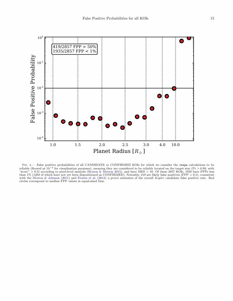
Fig. 4.— False positive probabilities of all CANDIDATE or CONFIRMED KOIs for which we consider the vespa calculations to bereliable (floored at 10−4 for visualization purposes), meaning they are considered to be reliably located on the target star (Pr > 0.99, with“score” > 0.3) according to pixel-level analysis (Bryson & Morton 2015), and have MES > 10. Of these 2857 KOIs, 1935 have FPPs lessthan 1% (1284 of which have not yet been dispositioned as CONFIRMED). Noteably, 419 are likely false positives (FPP > 0.5), consistentwith the Morton & Johnson (2011) and Fressin et al. (2013) a priori estimates of the overall Kepler candidate false positive rate. Redcircles correspond to median FPP values in equal-sized bins.

16 Morton et al.

Planet Radius [R⊕ ]

10-4

10-3

10-2

10-1

100F

als

e P

osi

tive

Pro

bab

ilit

y

1.0 2.0 3.0 10.0

1781/2533 FPP > 50%281/2533 FPP < 1%

Fig. 5.— Same as FIG. 4, but for KOIs currently dispositioned as FALSE POSITIVE. The vast majority are also identified by vespaas likely false positives. There are also some that have low FPPs, but this can be explained by the fact that many of the reasonsfor dispositioning a KOI as a FALSE POSITIVE also invalidate assumptions made by vespa; for example, that the signal is spatiallycoincident with the target star (see Section 4). This figure illustrates that vespa is effective (though not 100% efficient) at recovering knownfalse positives.

False Positive Probabilities for all KOIs 17

CONFIRMED (984)

FALSE POSITIVE (3168)

Calculation failed (100) MES < 10 (567)

Rp > 30 (278)

On-target probability < 0.99 or uncertain (516)

FPP > 0.9 (130)

0.01 < FPP < 0.9 (455)

FPP < 0.01 (1284)

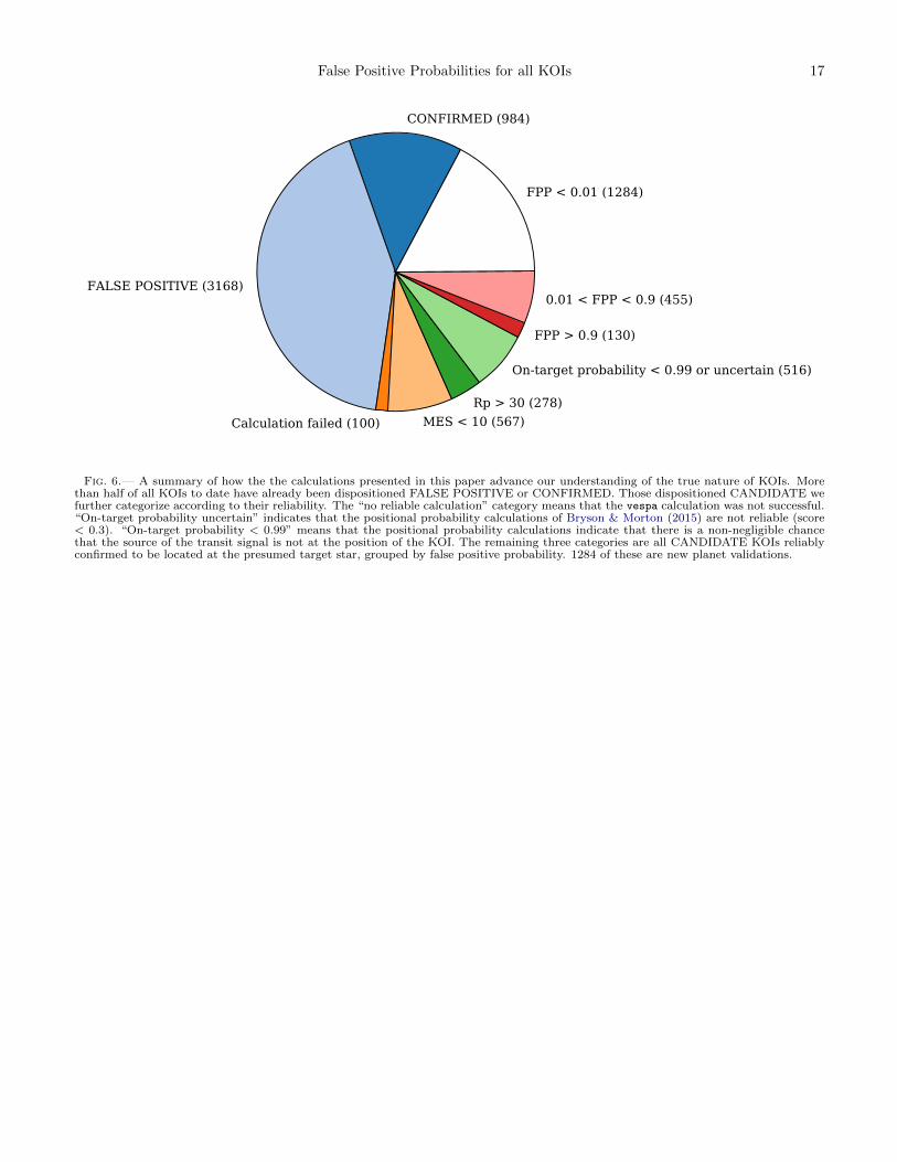
Fig. 6.— A summary of how the the calculations presented in this paper advance our understanding of the true nature of KOIs. Morethan half of all KOIs to date have already been dispositioned FALSE POSITIVE or CONFIRMED. Those dispositioned CANDIDATE wefurther categorize according to their reliability. The “no reliable calculation” category means that the vespa calculation was not successful.“On-target probability uncertain” indicates that the positional probability calculations of Bryson & Morton (2015) are not reliable (score< 0.3). “On-target probability < 0.99” means that the positional probability calculations indicate that there is a non-negligible chancethat the source of the transit signal is not at the position of the KOI. The remaining three categories are all CANDIDATE KOIs reliablyconfirmed to be located at the presumed target star, grouped by false positive probability. 1284 of these are new planet validations.

18 Morton et al.

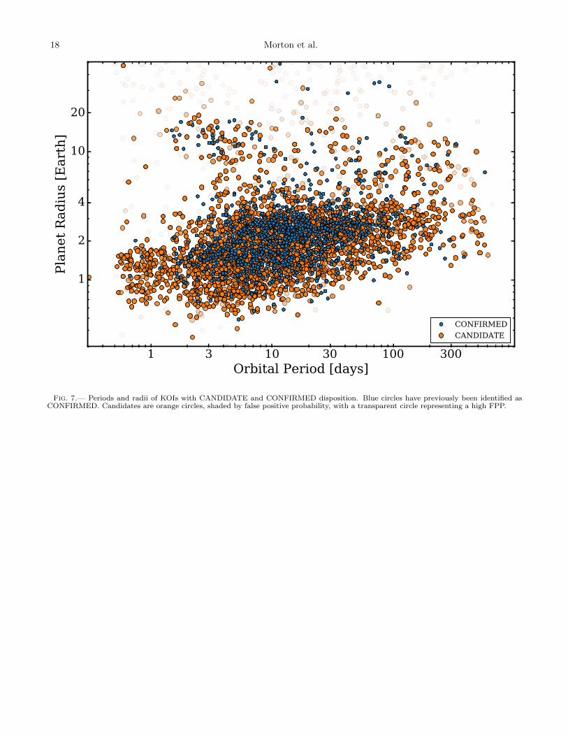
1 3 10 30 100 300Orbital Period [days]

1

2

4

10

20

Pla

net

Rad

ius

[Eart

h]

CONFIRMED

CANDIDATE

Fig. 7.— Periods and radii of KOIs with CANDIDATE and CONFIRMED disposition. Blue circles have previously been identified asCONFIRMED. Candidates are orange circles, shaded by false positive probability, with a transparent circle representing a high FPP.

False Positive Probabilities for all KOIs 19

3500

4000

4500

5000

5500

6000

6500

7000

7500

Eff

ect

ive T

em

pera

ture

[K

]

158/1212 inconsistent (13.0%)

0.5

1.0

1.5

2.0

2.5

3.0

3.5

4.0

Ste

llar

Rad

ius

[Sola

r]

55/1212 inconsistent (4.5%)

Fig. 8.— Comparison between temperatures and radii estimated from the isochrones analysis in this work and those from the Keplerstellar parameters catalog (H14), for the sample of stars hosting planets validated in this study. As seen in previous figures, the isochronesanalysis tends to over-predict the stellar radii compared to H14 for the coolest stars. A small number of stars are also estimated by thephotometric analysis of H14 to be evolved, but not by isochrones.

20 Morton et al.

TABLE

6False

PositiveProbabilityResu

lts

KO

IP

TT

V?

Rp

SN

Rδ s

ecar e

xclb

Pr E

Bc

Pr E

B2c

Pr H

EB

cP

r HE

B2c

Pr B

EB

cP

r BE

B2c

Pr b

oxy

dP

r long

dfp

ep

posfs p

osg

Dis

p.h

FP

Pi

σF

PP

jF

ailu

rek

Kep

l

(d)

(R⊕

)(p

pm

)(′′ )

K02360.0

12.3

04

N6.6

422.6

42

0.5

00

00

00

0.0

053

00.9

90.0

52

0.0

00.1

2F

P1

0–

–K

02361.0

15.7

84

N2.4

916.7

156

2.1

90.0

25

0.0

016

0.0

016

0.0

0026

0.0

095

0.0

054

00

0.2

01

1.0

00.2

5C

A0.0

43

0.0

026

––

K02362.0

12.2

37

N1.9

022.3

152

0.6

30

1.5

e-05

00

0.0

027

0.0

13

00

0.1

89

0.7

21.0

0F

P0.0

16

0.0

0047

––

K02362.0

211.0

85

N2.3

215.8

316

0.8

70.0

018

0.0

0013

8.8

e-05

1.6

e-05

0.0

0091

0.0

0018

00

0.2

15

1.0

00.6

4C

A0.0

031

0.0

0054

–1208b

K02363.0

13.1

39

N1.0

319.6

51

0.9

00

0.0

0025

02.7

e-05

0.0

29

0.0

15

00

0.1

01

1.0

00.8

8C

A0.0

44

0.0

016

––

K02364.0

15.2

42

N1.5

018.1

73

0.5

40

00

00

00.0

67

0.1

20.1

46

1.0

01.0

0C

A0.1

90.0

57

––

K02365.0

135.9

68

N1.9

819.4

81

1.4

40.0

20.0

004

0.0

0072

4.1

e-05

0.0

023

0.0

012

1.2

e-06

00.2

08

1.0

00.8

8P

L0.0

24

0.0

021

––

K02365.0

2110.9

74

N1.4

510.6

65

3.3

00

00

00.0

0031

4.1

e-05

0.0

01

00.1

45

1.0

00.5

9P

L0.0

013

0.0

001

––

K02366.0

125.3

69

N1.5

118.4

32

1.3

20.0

016

04.1

e-06

00

00.0

05

00.1

52

1.0

01.0

0C

A0.0

066

0.0

0055

–1209b

K02367.0

16.8

92

N1.4

016.4

25

2.1

60.0

66

0.0

22

0.0

15

0.0

03

0.4

20.4

10

00.1

37

1.0

00.9

9C

A0.9

40.0

029

––

K02368.0

18.0

71

N1.7

016.0

111

1.0

86.3

e-05

1.4

e-05

01.3

e-06

0.0

002

0.0

0011

2.3

e-06

00.1

77

1.0

00.6

2C

A0.0

004

4.7

e-05

–1210b

K02369.0

111.0

18

N2.5

518.3

138

0.7

80

00

01.3

e-05

08.2

e-06

00.2

02

1.0

00.9

9C

A2.2

e-05

4.8

e-06

–1211b

K02369.0

37.2

27

N1.3

27.5

116

2.2

20

00

02.6

e-05

0.0

0044

0.0

0015

1e-

05

0.1

30

0.8

60.3

3C

A0.0

0062

0.0

0012

––

K02370.0

178.7

32

N5.3

917.7

188

0.5

40.4

40.0

027

0.0

74

0.0

017

0.0

26

0.0

012

00

0.0

51

1.0

01.0

0C

A0.5

40.0

34

––

K02371.0

112.9

41

N2.1

419.4

85

1.7

48.1

e-05

00

02.3

e-05

01.1

e-05

00.2

12

1.0

00.9

9C

A0.0

0012

2.7

e-05

–1212b

K02372.0

15.3

50

N1.1

920.2

18

2.1

00

00

01.1

e-06

02.8

e-05

00.1

08

1.0

00.7

8C

A3e-

05

1.6

e-06

–1213b

K02373.0

1147.2

81

N2.1

913.5

176

2.8

80.0

0042

3.4

e-05

3.5

e-06

3.3

e-06

0.0

017

0.0

04

0.0

0019

00.2

16

0.9

71.0

0C

A0.0

064

0.0

0052

––

K02374.0

15.2

62

N1.3

018.5

56

0.7

50

00

00.0

0012

0.0

0016

1.1

e-05

1.3

e-06

0.1

32

1.0

00.8

8P

L0.0

0029

5.8

e-05

––

K02374.0

212.1

63

N1.4

814.8

138

2.5

20.0

012

0.0

04

6.2

e-06

0.0

0058

0.3

0.1

80

00.1

53

1.0

00.5

6P

L0.4

90.0

055

––

K02375.0

140.8

79

N2.0

018.4

109

2.4

90

0.0

0026

06.9

e-06

0.4

0.6

00

0.2

09

0.0

10.0

6F

P0.9

90.0

024

––

K02376.0

118.8

26

N2.3

617.1

229

1.2

30.0

021

4.1

e-06

9.7

e-06

08.3

e-05

4.3

e-06

1.1

e-05

00.2

14

1.0

00.9

0C

A0.0

023

0.0

0063

–1214b

K02377.0

113.9

03

N1.5

015.0

131

0.9

02e-

05

2.2

e-06

01.5

e-06

0.0

025

0.0

0065

2e-

06

00.1

51

0.0

70.8

8C

A0.0

031

0.0

0012

––

K02378.0

14.7

67

N1.2

212.8

65

1.2

30

6.4

e-05

02.3

e-05

0.0

024

0.0

0051

3.6

e-06

00.1

21

1.0

00.6

4C

A0.0

031

0.0

0016

–1215b

K02379.0

140.0

09

N80.5

417.8

553

1.2

90.3

40.0

61

0.0

26

0.0

089

0.3

70.2

00

0.0

01

1.0

00.9

8F

P1

0–

–K

02380.0

16.3

57

N1.9

315.6

102

0.7

80.0

33

0.0

14

0.0

027

0.0

019

0.0

14

0.0

14

1.4

e-06

00.2

19

1.0

00.9

7C

A0.0

81

0.0

057

––

Note.

—A

port

ion

of

this

table

issh

ow

nfo

rfo

rmand

conte

nt.

The

full

table

will

be

available

online.

aM

axim

um

secondary

eclipse

depth

allow

ed.

b“E

xclu

sion

radiu

s”in

side

of

whic

hfa

lse

posi

tive

scenari

os

are

allow

ed.

cP

robabilit

ies

for

diff

ere

nt

ast

rophysi

cal

fals

ep

osi

tive

scenari

os:

unble

nded

eclipsi

ng

bin

ary

(EB

),hie

rarc

hic

al

eclipsi

ng

bin

ary

(HE

B),

and

back

gro

und/fo

regro

und

eclipsi

ng

bin

ary

(BE

B).

”2”

indic

ate

sdouble

-peri

od

scenari

o.

dA

rtifi

cia

lm

odels

toid

enti

fysi

gnals

that

are

poorl

ydesc

rib

ed

by

any

of

the

ast

rophysi

cal

scenari

os.

eA

ssum

ed

“sp

ecifi

cpla

net

occurr

ence

rate

”fo

rth

ispla

net.

fP

robabilit

yof

signal

tob

eon

targ

et

star,

accord

ing

toB

ryso

net

al.

(2015,

inpre

p).

gP

osi

tional

pro

babilit

ysc

ore

,fr

om

Bry

son

et

al.

(2015).

hE

xopla

net

Arc

hiv

edis

posi

tion:

fals

ep

osi

tive

(FP

),candid

ate

(CA

),or

confirm

ed

(PL

).i

Fals

ep

osi

tive

pro

babilit

y;

mean

of

10

boots

trap

recalc

ula

tions.

jFals

ep

osi

tive

pro

babil

ity

uncert

ain

ty;

standard

devia

tion

of

10

boots

trap

recalc

ula

tions.

kR

easo

nfo

rfa

ilure

:(1

)N

oM

CM

Cm

odeling

available

from

Row

eet

al.

(2015);

(2)

Unphysi

cal

MC

MC

fit

from

Row

eet

al.

(2015);

(3)

No

stellar

para

mete

rsavailable

from

Hub

er

et

al.

(2014);

(4)

No

weak

secondary

data

available

;(5

)M

CM

Ctr

ap

ezoid

fit

did

not

converg

e;

(6)

Peri

od

too

short

for

implied

star

(orb

itw

ithin

star)

;(7

)O

ther

unsp

ecifi

edvespa

err

or.

lK

eple

rnum

ber

ass

igned,

ifvalidate

d.