Title An exact WKB approach to the 2-level adiabatic transitionproblems(Spectral and Scattering Theory and Related Topics)

Author(s) Watanabe, Takuya

Citation 数理解析研究所講究録 (2006), 1510: 8-25

Issue Date 2006-07

URL http://hdl.handle.net/2433/58588

Right

Type Departmental Bulletin Paper

Textversion publisher

Kyoto University

An exact WKB approach to the 2-1eveladiabatic transition problems

Takuya Watanabe (渡部拓也)Mathematical Institute, Tohoku University (東北大学大学院理学研究科)

1 Introduction

We consider the time-dependent Schr\"odinger equation:

$ih \frac{d}{dt}\psi(t)=\mathcal{H}(t.\epsilon)\psi’(t\rangle$ , $\mathcal{H}(t,\epsilon)=(V(t)\epsilon$ $-V(t)\epsilon)$ (1)

on $\mathrm{R}$ , where $\epsilon$ and $h$ are small positive parameters and $V(t)$ is a real-valued function. $\psi(t)$

is a vector-valued function with complex components. This equation (1) describes theadiabatic time evolution associated to the Hamiltonian $\mathcal{H}(_{b_{d}^{\wedge}}, h)$ . This 2 $\mathrm{x}2$ real symmetricand trace-free matrix $\mathcal{H}(\epsilon, h)$ has two real eigenvalues $E_{3_{\sim}^{\sim}}(t,\epsilon)=\pm\sqrt{V(t)^{2}+\epsilon^{2}}$ . Thedifference of these eigenvalues

$E_{+}-E_{-}=‘ 2\sqrt{V(t)^{2}+\epsilon^{2}}$

is strictly positive for all $t\in \mathrm{R}$ and has its minimum $2\hat{\epsilon}$ at the zeros of $V(t)$ .From the physical point of view, the two different unperturbed energy levels $V(t)$ and

$-V(t)$ cross each other at the zeros of $V(t)$ and $\tilde{\epsilon}$ is the interaction at the intersection.Because of this interaction, $E_{+}(t,\epsilon)$ and $F_{J}-(t,\tau.)$ do not cross (avoided crossing), but thetransition occurs by the quantum effect. The parameter $h$ is the adiabatic parameter andthe quantum effect becomes small in the adiabatic limit. On the other hand, $-C$ is the gapat the avoided crossing. One expects, then, that the transition probability $P(\epsilon, h)$ is smallwhen $h$ is small while it is large when $.c$ is small. It is an interesting problem to study itsasymptotic behavior as both $\vee c$ and $h$ go to $0$ .

The study of the transition probability $P$ has its origin at the works by L. D. Landau[L] and C. Zener [Z]. In 1932, they studied the case $V(t)=at,$ where $a$ is a positiveconstant, and derived the following explicit formula:

$P= \exp[-\frac{\pi^{c^{2}}}{ah}\vee]$

for all positive $\vee c$ and $h$ . This is the so-called Landau-Zener formula. There have been manystudies about the transition probability in the adiabatic limit $harrow \mathrm{O}$ (see the summaries[BT]. [HJ], [T] $)$ . The adiabatic limit of the transition probability is expressed in terms ofactions between complex eigenvalue crossing points:

$\{t\in \mathbb{C} ; V(t)^{2}+W(t)^{2}=0\}$ ,

which we call turning points.

数理解析研究所講究録1510巻 2006年 8-25 8

In this proceeding we consider more general $V(t)$ which vanishes at one point to order$n$ , and compute the asymptotic behavior of $P(\epsilon, h)$ as $(\epsilon, h)arrow(\mathrm{O},0)$ under the condition$h/\epsilon^{(n+1)/n}arrow 0$ . In case $n=1$ , this problem is studied in more general settings by [CLP]and [Ro].

Recently new approaches of an exact WKB method have been studied. These ap-proaches give the rigorous argument to the divergent power series solution on the singularperturbation $h$ . [AKT] studied the Hamiltonian, which is 3 $\mathrm{x}3$ real symmetric matrix withpolynomial elements, by the exact WKB method based on the Borel resummation. In thispaper we apply the exact WKB method developed by C.G\’erard and A.Grigis [GG], andS.Fujii\’e, C.Lasser and L.Nedelec [FLN] to this adiabatic transition problem. This methodenables us to express the Wronskian of two exact WKB solutions as a convergent seriesdefined inductively by integrations along a path. Careful observations of the phase func-tion on the path gives us their asymptotic behavior of the Wronskian as $(\epsilon_{!}.h)arrow(\mathrm{O},0)$

with $h/\epsilon^{(n+1)/n}arrow 0$ .Finally we remark that this is similar to the scattering problem for Schr\"odinger oper-

ator over the maximum of the potential. See [Ra], [FR] for a non-degenerate maximumcase and [BM] for a degenerate maximum case.

2 Definitions and ResultsWe first define the scattering matrix and the transition probability for the equation (1)under the following assumptions on $V(t)$ :

(A) $V(t)$ is real valued on $\mathrm{R}$ and there exist two real numbers $0<\theta_{0}<\pi/2$ and $\rho>0$

such that $V(t)$ is analytic in the complex domain:

$S=\{t\in \mathbb{C} ; |{\rm Im} t|<|{\rm Re} t|\tan\theta_{0}\}\cup\{|{\rm Im} t|<\rho\}$ .

(B) There exist two real non-zero constants $E_{r},$ $E_{l}$ and $\sigma>1$ such that

V $(t)=\{$$E_{r}+O(|t|^{-\sigma})$ as ${\rm Re} t\overline,$ $+\infty$ in $S$ ,

$E_{l}+O(|t|^{-\sigma})$ as ${\rm Re} tarrow-\infty$ in $S$ .

Under the conditions (A) and (B), there exist four solutions th$r+\cdot\psi_{-}^{r},$ $\psi_{\vdash}^{l}$ , and $\psi_{-}^{l}$ to(1) uniquely defined by the following asymptotic conditions:

$\{$

$\psi_{+}^{f}(t)\sim\exp[+\frac{i}{h}\sqrt{E_{f}^{2}+\epsilon^{2}}t]$ , as ${\rm Re} tarrow+\infty$ in $S$ ,

$\psi_{-}^{r}(t)\sim\exp[-\frac{i}{h}\sqrt{E_{r}^{2}+\epsilon^{2}}t]$ , as $\mathrm{R}\epsilon tarrow+\infty$ in $S$ ,

$\psi_{+}^{l}(t)\sim\exp[+\frac{i}{h}\sqrt{E_{l}^{2}+\vee^{-2}\llcorner}\iota]$ , as ${\rm Re} tarrow-\infty$ in $S$ ,

$\psi_{-}^{l}(t)\sim\exp[-\frac{i}{h}\sqrt{E_{l}^{2}+\epsilon^{2}}t]$ . as ${\rm Re} tarrow-\infty$ in $S$ ,

(2)

9

where $\tan 2\theta_{r}=\epsilon/E_{r}$ and $\tan 2\theta_{l}=\vee^{\wedge}\vee/E_{l}(0<\theta_{r}.\theta_{l}<\pi/2)$ . These solutions are calledJost solutions to (1). We notice that the principal term of each Jost solution, for example$\exp[+\frac{i}{h}\sqrt{E_{r}^{2}+\epsilon^{2}}t]{}^{t}(-\sin\theta_{r}\cos\theta_{r})$. is a solution to the constant coefficient system:

$ih \frac{d}{dt}\psi(t)=\psi(t)$ .

The pairs of Jost solutions $(\psi_{+}^{f},\psi_{-}’)r.$ and $(\psi_{+}^{l}, \psi_{-}^{l})$ are orthonormal bases on $\mathbb{C}^{2}$ for anyfixed $t$ . Moreover they have the following relations:

$\psi_{\pm}^{f}(t)=\mp\overline{\psi_{+}^{r}(t)}$ , $\psi_{\pm}^{l}(t)=\mp\overline{\psi_{\mp}^{l}(t)}$ . (3)

The scattering matrix $S$ is defined as the change of bases of Jost solutions:

$(\psi_{+}^{l}\psi_{-}^{l})=(\psi_{+}^{r}\psi_{-}^{r})S(\hat{\in}, h)$ , $S(\epsilon, h)=$ .

$S$ is an unitary matrix independent of $t$ and moreover, by (3),

$s_{11}(\epsilon, \mathrm{h})=s_{22}(- h\vee)’,$ , $s_{12}(\epsilon, h)=-\overline{s_{21}(\epsilon,h)}$.The transition probability $P(\epsilon.h)$ is defined by

$P(\overline{\epsilon},h)=|s_{21}(\epsilon, h)|^{2}$ .

Let us assume

(C) V$(t)=0$ if and only if $t=0$ .

Then the eigenvalues have the so-called avoided crossing at the origin. We call turningpoint a complex zero of V $(t)^{2}+_{\vee}c^{2}$ , and in particular, simple turning point if it is a simplezero.

Let $n\in \mathrm{N}=\{1,2, \cdots\}$ be the number such that $V^{(k)}(0)=0$ for $0\leq k<n$ and$V^{(n)}(0)\neq 0$ . We can assume $V^{(n)}(0)>0$ without loss of generality. Then there are $2n$

simple turning points $T_{j}(\epsilon)$ and $\overline{T_{j}(\hat{\epsilon})}(j=1, \ldots , n)$ with $0<\arg T_{1}<\cdots<\arg T_{n}<\pi$

which converge at the origin as $\epsilon$ tends to $0$ . We define the action integral $A_{j}(\epsilon)$ by,

$A_{j}(_{\dot{\mathrm{c}}}^{\backslash })=2 \int_{0}^{T_{j}(\epsilon)}\sqrt{V(t)^{2}+\epsilon^{2}}dt$,

where the integration path is the complex segment from $0$ to $T_{j}(\in\rangle$ and the branch of thesquare root is $\epsilon$ at $t=0$ . Our main result is the following asymptotic formula of $P(\epsilon, h)$

when $\epsilon$ and $h$ are both small.

Theorem 2.1. Assum,$e(\mathrm{A}),$ $(\mathrm{B})$ , and (C). If $n=1$ there exists $\epsilon_{0}>0$ such that rv$e$

have$P( \epsilon,h)=\exp[-‘\frac{2\mathrm{I}\mathfrak{n}\iota A_{1}(\overline{\mathrm{a}})}{h}](1+O(h))$ as $harrow 0$

10

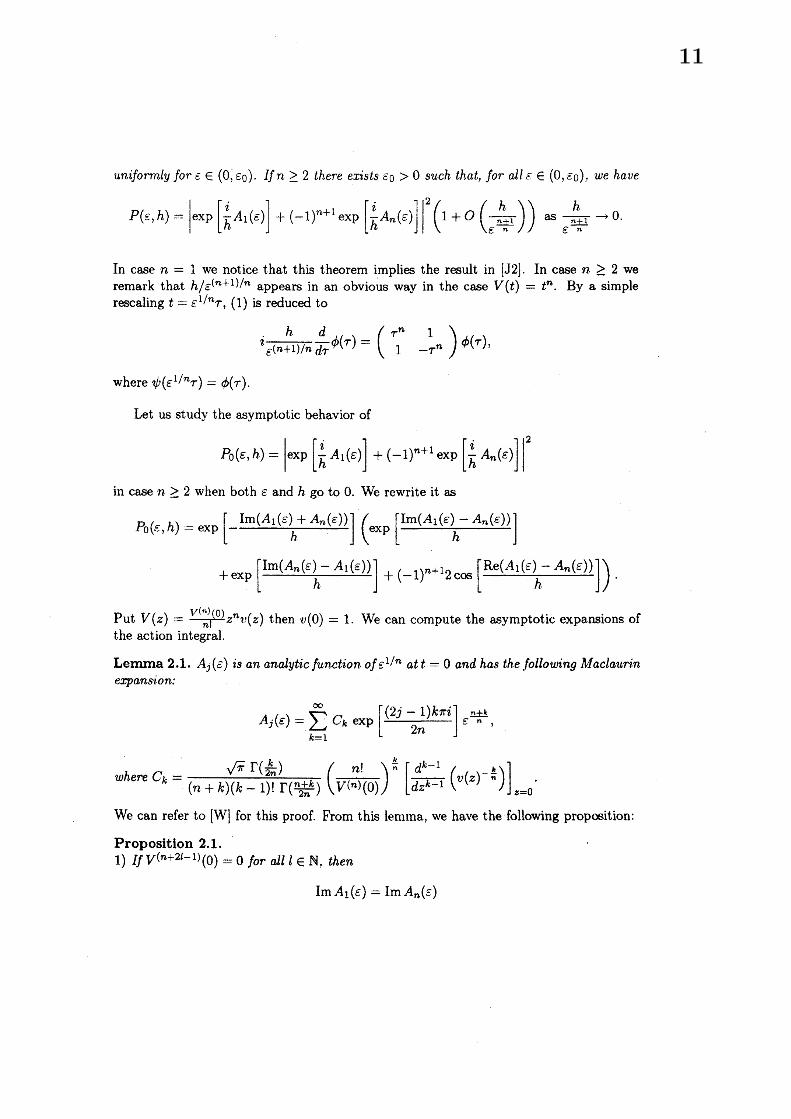
uniformly $for\overline{\vee\succ}\in(0, \epsilon 0)$ . If $n\geq 2$ there exists $\epsilon_{0}>0$ such that, for all $\epsilon\in(0,4\vee^{\wedge}0)$ . we have

$P(^{-}. \cdot, h)=|\exp[\frac{?}{h}A_{1}(\epsilon)]+(-1)^{n+1}\exp[\frac{i}{h}A_{n}(\epsilon)]|^{2}(1+O(\frac{h}{\epsilon^{\frac{n+1}{n}}}))$ as $\frac{h}{\epsilon^{\frac{n+1}{n}}}arrow 0$ .

In case $n=1$ we notice that this theorem implies the result in [J2]. In case $n\geq 2$ weremark that $h/\epsilon^{(n+1)/n}$ appears in an obvious way in the case $V(t)=t^{n}$ . By a simplerescaling $t=\epsilon^{1/n}\tau,$ (1) is reduced to

$i \frac{h}{\epsilon^{(n+1)/n}}\frac{d}{d\tau}\phi(\tau)=\phi(\tau)$ ,

where $\psi(\epsilon^{1/n}\tau)=\phi(\tau)$ .

Let us study the asymptotic behavior of

$P_{0}( \epsilon, h)=|\exp[\frac{i}{h}A_{1}(\epsilon)]+(-1)^{n+1}\exp[\frac{i}{h}A_{n}(\epsilon)]|^{2}$

in case $n\geq 2$ when both $\epsilon$ and $h$ go to $0$ . We rewrite it as

$P_{0}( \in, h)=\exp[-\frac{{\rm Im}(A_{1}(\epsilon)+A_{n}(\epsilon))}{h}](\exp[\frac{{\rm Im}(A_{1}(\epsilon)-A_{n}(\Xi))}{h}]$

$+ \exp[\frac{{\rm Im}(A_{n}(_{\vee}^{\mathrm{r}})-A_{1}(\Xi))}{h}]+(-1)^{n+1}2$coe $[ \frac{{\rm Re}(A_{1}(\epsilon)-A_{n}(\epsilon))}{h}])$ .

Put $V(_{\sim}’)= \frac{\mathrm{t}\gamma(n\prime(0)\backslash }{n\mathrm{I}}z^{n}v(z)$ then $v(\mathrm{O})=1$ . We can compute the asymptotic expansions ofthe action integral.

Lemma 2.1. $A_{j}(\epsilon)$ is an analytic fun.ction of $\overline{\epsilon}^{1/n}$ at $t=0$ and has th.$e$ following Madaurinexpansion:

$A_{j}( \epsilon)=\sum_{k=1}^{\infty}C_{k}\exp[\frac{(2j-1)k\pi i}{2n}]\epsilon^{\frac{n+k}{n}}$

where $C_{k}= \frac{\sqrt{\pi}\Gamma(\frac{k}{2n}\rangle}{(n+k)(k-1)!\Gamma(\frac{n+k}{2n})}(\frac{n!}{V^{(n)}(0)})^{\frac{k}{n}}[\frac{d^{k-1}}{d_{\tilde{k}}k-1}(v(z)^{-\frac{k}{\mathfrak{n}}})]_{z=0}$

We can refer to [W] for this proof. From this lemma, we have the following proposition:

Proposition 2.1.1) If $V^{(n+2l-1)}(0)=0$ for all $l\in \mathrm{N}$ . then

${\rm Im} A_{1}(\epsilon)={\rm Im} A_{n}(-.)$’

11

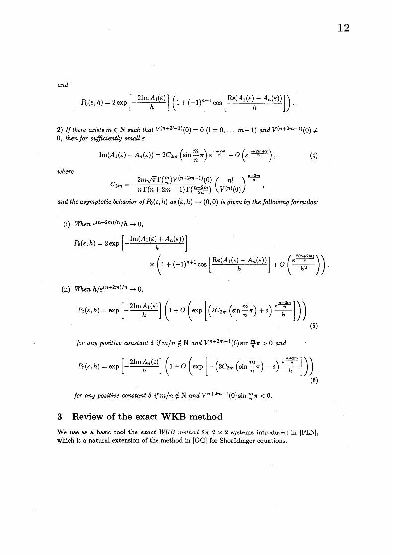
and

$P_{0}( \circ, h\mathrm{c})=2\exp[-\frac{2{\rm Im} A_{1}(\epsilon)}{h}](1+(-1)^{n+1}\cos[\frac{{\rm Re}(A_{1}(\epsilon)-A_{n}(\epsilon))}{h}])$ .

2) If th.$ere$ eansts $m\in \mathrm{N}$ such that $V^{(n+2l-1)}(0)=0(l=0, \ldots, m-1)$ and $V^{(n+2m-1)}(0)\neq$

$0$ , then for sufficiently small $\epsilon$

${\rm Im}(A_{1}( \epsilon)-A_{n}(\epsilon))=2C_{2m}(\sin\frac{m}{n}\pi)\epsilon^{\frac{n+2m}{n}}+O(\epsilon^{\frac{n+2m+2}{n}})$ , (4)

where

$C_{2m}=- \frac{2m\sqrt{\pi}\Gamma(\frac{m}{n})V^{(n+2m-1)}(0)}{n\Gamma(n+2m+1)\Gamma(\frac{n+2m}{2n})}(\frac{n!}{V^{(n)}(0)})^{\frac{n+2m}{n}}$ ,

and the asymptotic behavior $ofP_{0}(\epsilon, h)$ as $(\epsilon, h)arrow(\mathrm{O}, 0)$ is given by the following formulae:

(i) When $\epsilon^{(n+2m)/n}/harrow 0$,

$P_{0}( \epsilon,h)=2\exp[-\frac{{\rm Im}(A_{1}(\epsilon)+A_{n}(\epsilon))}{h}]$

$\mathrm{x}(1+(-1)^{n+1}\cos[\frac{{\rm Re}(A_{1}(\epsilon\rangle-A_{n}(\epsilon))}{h}]+O(\frac{\epsilon^{\frac{2(n+2n)}{n}}}{h^{2}}))$

(ii) When $h/\epsilon^{(n+2m)/n}arrow 0$ ,

$P_{0}( \epsilon, h)=\exp[-\frac{2{\rm Im} A_{1}(\epsilon)}{h}](1+O(\exp[(2C_{2m}(\sin\frac{m}{n}\pi)+\delta)\frac{\epsilon^{\frac{n+2m}{n}}}{h}]))$

(5)

for any positive constant 6 $ifm/n\not\in \mathrm{N}$ and $V^{n+2m-1}(0) \sin\frac{m}{n}\pi>0$ and

$P_{0}( \epsilon^{-}, h)=\exp[-\frac{2{\rm Im} A_{n}(\epsilon)}{h}](1+O(\exp[-(2C_{2m}(\sin\frac{m}{n}\pi)-\delta)\frac{\epsilon^{\frac{n+2m}{n}}}{h}]))$

(6)

for any positive constant 6 if $m/n\not\in \mathrm{N}$ and $V^{n+2m-1}(0) \sin\frac{m}{n}\pi<0$ .

3 Review of the exact WKB method

We use as a basic tool the exact $WKB$ method for 2 $\mathrm{x}2$ systems introduced in [FLN],which is a natural extension of the method in [GG] for Shor\"odinger equations.

12

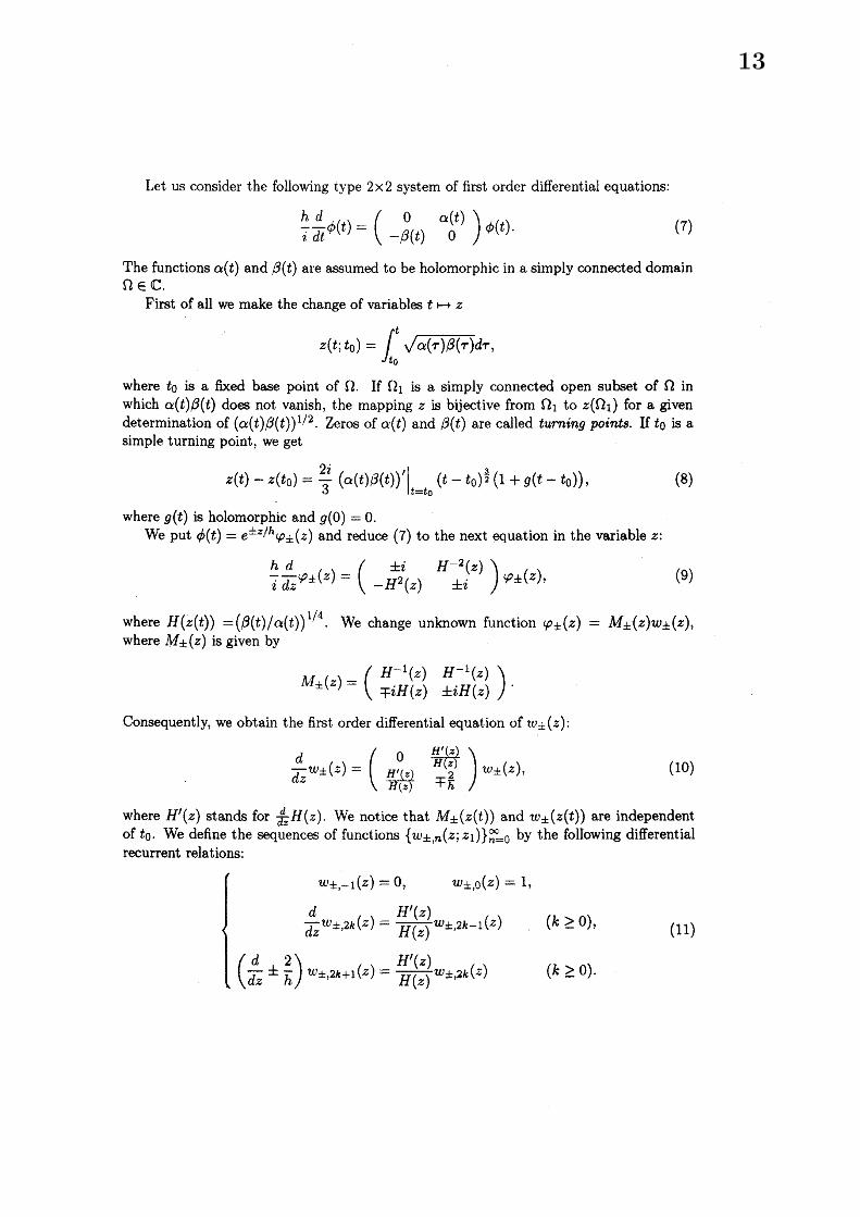
Let us consider the following type $2\cross 2$ system of first order differential equations:

$\frac{h}{i}\frac{d}{dt}\phi(t)=\phi(t)$ . (7)

The functions $\alpha(t)$ and $\beta(t)$ are assumed to be holomorphic in a simply connected domain$\Omega\in$ C.

First of all we make the change of variables $trightarrow z$

$z(t;t_{0})= \int_{t_{0}}^{t}\sqrt{\alpha(\tau)\beta(\tau)}d\tau$ ,

where $t_{0}$ is a fixed base point of St. If $\Omega_{1}$ is a simply connected open subset of $\Omega$ inwhich $\alpha(t)\beta(t)$ does not vanish, the mapping $z$ is bijective from $\Omega_{1}$ to $z(\Omega_{1})$ for a givendetermination of $(\alpha(t)\beta(t))^{1/2}$ . Zeros of $\alpha(t)$ and $\beta(t)$ are called turreing points. If $t_{0}$ is asimple turning point, we get

$z(t)-z(t_{0})= \frac{2i}{3}(\alpha(t)_{}\theta(t))’|_{t=t_{0}}(t-t_{0})^{\frac{3}{2}}(1+g(t-t_{0}))$, (8)

where $g(t)$ is holomorphic and $g(\mathrm{O})=0$ .We put $\phi(t)=e^{\perp_{z/h}}"\varphi_{\mathrm{x}}(z)$ and reduce (7) to the next equation in the variable $z$ :

$\frac{h}{i}\frac{d}{d_{\wedge}\sim}\varphi\pm(z)=\varphi\pm(z)$ , (9)

where $H(z(t))=(\theta(t)/\alpha(t))^{1/4}$ We change unknown function $\varphi\pm(z\rangle=M_{\pm}(z)w\pm(z)$ ,where $M_{\pm}(z)$ is given by

$\Lambda I_{\pm}(z)=$ .

Consequently, we obtain the first order differential equation of $\mathrm{c}\iota_{\pm}’(z)$ :

$\frac{d}{d_{\tilde{4}}}w_{\pm}(z)=(\neq_{\langle z)}^{0}H’z\mathit{1}$ $\frac{H’(z)}{H(z),\mp_{\mathrm{F}}^{2}})w_{\pm}(z)$ , (10)

where $H’(z)$ stands for $\frac{d}{dz}H(z)$ . We notice that $M_{\pm}(\approx(t))$ and $w_{\pm}(z(t))$ are independentof $t_{0}$ . We define the sequences of functions $\{u_{\pm,n}’(z:, z_{1})\}_{n=0}^{\infty}$ by the following differentialrecurrent relations:

$\{$

$\mathrm{e}\iota|\pm,-\iota(z)=0$ , $w_{\pm,0}(z)=1$ ,

$\frac{d}{dz}w_{\neq,2k}(z)=\frac{H’(_{\sim})}{H(z)},w_{\pm,2k-1}(z)$ $(k\geq 0)$ ,

$( \frac{d}{dz}\pm\frac{2}{h})w_{\pm,2k+1}(z)=\frac{H’(z)}{H(\sim\prime)}w_{\pm,2k}(z)$ $(k\geq 0)$ .

(11)

13

The vector-valued functions $w\pm(z(t))=$ with

$u_{\pm}^{e}’(z(t))= \sum_{k\geq 0}w\pm,2k(z(t))$,

satisfy (10) formally.$H’(z)/H(z)$ is, in terms of $t$ ,

$w_{\pm}^{o}(z(t))= \sum_{k\geq 0}w_{\pm,2k-1}(z(t)\rangle$ .

$\frac{d{}_{\tau z}H(z(t\rangle)}{H(z(t))}=\frac{\alpha(t)\beta’(t)-\alpha’(t)\beta(t)}{4i(\alpha(t)\beta(t))^{3/2}}$ . (12)

From (8) and (12), we see that $H’(z)/H(z)$ has a simple pole at $z=z(t_{0})$ .We fix a point $z_{1}=z(t_{1})$ with $t_{1}\in\Omega_{1}$ and take the initial conditions to $w_{\pm,n}(z_{1})=0$

for every $n\in$ N. Then the differential recurrent equations (11) are transformed to theintegral recurrent equations:

$\{$

$w_{\pm,0}(z;z_{1})=1$ ,

$w_{\pm,2k+1}(z;z_{1})= \int_{z_{1}}^{z}e^{\pm\frac{2}{h}(\zeta-z)}\frac{H’(\zeta)}{H(\zeta)}u_{\pm,2k}’(\zeta;z_{1})d\zeta$ $(k\geq 0)$ ,

$w_{\pm,2k}(z;z_{1})= \int_{z_{1}}^{z}\frac{H’(\zeta)}{H(\zeta)}w_{\pm,2k-1}(\zeta;z_{1})d\zeta$ $(k\geq 1)$ .

From these integral representations, we obtain the following proposition on the convergenceof these formal series.

Proposition 3.1. Th.e elements of the function, $w_{\pm}(z;z_{1})$ :

$w_{\pm}^{e}(z;z_{1})= \sum_{k\geq 0}w_{\pm,2k}(z;z_{1})$ $w_{\pm}^{o}(z;z_{1})= \sum_{k\geq 0}w_{\pm,2k-1}(z;z_{1})$(13)

converge absolutely and uniformly in a neighborhood of $z=z_{1}$ .

Hence $nj+(z_{\backslash }z\iota)$ are exact solutions to the equation (10) and

$\phi_{\pm}(t, h;t_{0},t_{1})=e^{\pm z(t;t_{0})/h}hf_{\pm}(z(t))w_{\pm}(z(t\rangle, h;z(t_{1}))$. (14)

define exact solutions to (7). We call $\emptyset\pm(t, h;t_{0},t_{1})$ exact $WKB$ solutions. (14) are holo-morphic in a neighborhood of $t=t_{1}$ , and extended to $\Omega$ analytically because (14) satisfy(7) with the holomorphic coefficients in $\Omega$ . We call $t_{0}$ the base point of the phase and $t_{1}$

the base point of the symbol.The series (13) are also asymptotic expansions as $harrow \mathrm{O}$ in certain domains.

14

Proposition 3.2. There exist a positive integer $N$ and a positive constant $h_{0}$ such that,for all $h\in(\mathrm{O}, h_{0})_{j}$ we have

$w_{\pm}^{e}(z(t), h;z(t_{1}))- \sum_{k=0}^{N-1}v_{\pm,2k}’(z(t), h;z(t_{1}))$ $=O(h^{N})$ ,

$w_{\pm}^{o}(z(t), h;z(t_{1}))- \sum_{k=0}^{N-1}u_{\pm,2k-1}’(z(t), h;z(t_{1}))=O(h^{N+1})$ ,

$unifo7mly$ in $\Omega_{\pm}$ , where $\Omega_{\pm}=\{t\in\Omega_{1}$ ; there erists a curve from $t_{1}$ to $t$ along which$\pm{\rm Re} z(t)$ increases strictly}.

Moreover the Wronskian between two exact WKB solutions $\mathcal{W}[\phi(t),\tilde{\phi}(t)]=\det(\phi(t)\tilde{\phi}(t))$

is given by $w_{+}^{e}:$

Proposition 3.3. Linearly independent exact $WKB$ solutions $\phi_{+}(t, h;t_{0}, t_{1})$ and$\phi_{-}(t, h;t_{0}, t_{2})$ satisfy the $follo\dot{w}ng$ Wronskian formula:

$\mathcal{W}[\phi_{+}(t, h;t_{0},t_{1}), \phi_{-}(t, h;t_{0}.t_{2})]=2iw_{+}^{e}(z(t_{2});z(t_{1}))$.

In particular, if there $e$ rists a curve from $t_{1}$ to $t_{2}$ along which ${\rm Re} z(t)$ increases strictly,

$\mathcal{W}[\phi_{+}(t, h, t_{0}, t_{1}), \phi_{-}(t, h;t_{0}.t_{2})]=2i(1+O(h))$ .

Notice that the Wronskian is independent of the variable $t$ because the matrix of right-handside of (7) is trace-free. The latter claim is evident from Proposition 3.2.

4 Stokes geometry

We introduce the so-called Stokes line. which plays an important role in our problem.

Deflnition 4.1 (Stokes line). The Stokes lines passing by $t=t_{0}$ in $S$ are defin.$ed$ as theset:

$\{t\in S$ ; ${\rm Im} \int_{t_{0}}^{t}\sqrt{V(\tau)^{2}+\epsilon^{2}}d\tau=0\}$ .

A Stokes line is a level set of the real part of the WKB phase function $z(t:t_{0})$ referringto (16). The turning points are the branch points of $z(t;t_{0})$ . If ${\rm Re} z(t)$ increases alongan oriented curve, then this curve is transversal to Stokes lines. Such a curve is calledcanonical curve.

We first state the local properties of Stokes lines near a fixed point $t_{0}\in S$ .

(i) If to is not a turning point, then $z(t;t_{0})$ is conformal near $t=t_{0}$ .

(ii) If $t_{0}$ is a turning point of order $r\in$ N. that is $V(t)^{2}+\epsilon^{2}=(t-t_{0})^{r}\dot{V}(t)$ with$\tilde{V}(0)\neq 0$ . then there exist $r+2$ Stokes lines emanating from $t=t_{0}$ and every anglebetween two closest Stokes lines is $2\pi/(r+2)$ at $t=t_{0}$ .

15

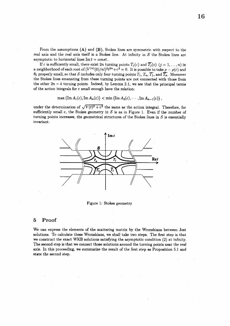
From the assumptions (A) and (B), Stokes lines are symmetric with respect to thereal axis and the real axis itself is a Stokes line. At infinity in $S$ the Stokes lines areasymptotic to horizontal lines ${\rm Im} t=const.$ .

If $\epsilon$ is sufficiently small, there exist $2n$ turning points $T_{j}(\overline{\epsilon})$ and $\overline{T_{j}}(\in)(j=1, \ldots , n)$ ina neighborhood of each root of $(V^{(n)}(0)/n!)^{2}t^{2n}+\tau^{2}.=0$ . It is possible to take $\rho=\rho(\epsilon)$ and$\theta_{0}$ properly small, so that $S$ includes only four turning points $T_{1},$ $T_{n},$ $\overline{T_{1}}$, and $T_{n}$ . Moreoverthe Stokes lines emanating from these turning points are not connected with those fromthe other $2n-4$ turning points. Indeed, by Lemma 2.1. we see that the principal termsof the action integrals for $\epsilon$ small enough have the relation:

$\max\{{\rm Im} A_{1}(\epsilon),{\rm Im} A_{n}(\epsilon)\}<\min\{{\rm Im} A_{2}(\epsilon), \cdots,{\rm Im} A_{n-1}(\epsilon)\}$ ,

under the determination of $\sqrt{V(t\rangle^{2}+\epsilon^{2}}$ the same as the action integral. Therefore, forsufficiently small $\epsilon$ , the Stokes geometry in $S$ is as in Figure 1. Even if the number ofturning points increases, the geometrical structures of the Stokes lines in $S$ is essentiallyinvariant.

Figure 1: Stokes geometry

5 Proof

We can express the elements of the scattering matrix by the Wronskians between Jostsolutions. To calculate these Wronskians, we shall take two steps. The first step is thatwe construct the exact WKB solutions satisfying the asymptotic condition (2) at infinity.The second step is that we connect those solutions around the turning points near the realaxis. In this proceeding, we summarize the result of the first step as Proposition 5.1 andstate the second step.

16

First of all, by the change of the unknown function $\psi’(t)=Q\phi(t),$ $Q= \frac{1}{2}$ ,

(1) is reduced to an equation of the form (7):

$\frac{h}{i}\frac{d}{dt}\phi(t)=\phi(t)$ . (15)

In this case, the phase function $z(t;t_{0})$

$z(t;t_{0})=? \int_{t_{0}}^{t}\sqrt{V(\tau)^{2}+\epsilon^{2}}d\tau$ $(t_{0}\in S)$ . (16)

Recalling that we take the branch of $\sqrt{V(t)^{2}+\epsilon^{2}}$ which is $\epsilon$ at $t=0$ . we aee that ${\rm Re} z(t)$

increases as ${\rm Im} t$ decreases, and ${\rm Im} z(t)$ increases as ${\rm Re} t$ increases around the real axis.Similarly the branch of

$H\langle z(t))=\sqrt[4]{\frac{iV(t)+\sigma}{iV(t)-\vee c}=}$.

is $e^{\pi/4}$ at $t=0$ . We introduce four symbol base points $r_{+},$ $r_{-},$ $l_{+},$ $l$ -and make the branchcuts as in Figure 2. We write, for short, the exact WKB solutions by

$\emptyset\pm(t, h;T_{j},t_{1})=\phi_{\pm}^{(J)}(t_{1})$ . $\emptyset\pm(t, h;T_{j}, t_{1})=\phi_{\pm}^{(\overline{j})}(t_{1})$ ,

because the Wronskian calculation is independent of $t$ . Then we sum the first step asfollows:

Figure 2: symbol base points

17

Proposition 5.1. We obtain the following relations between the Jost solutions and theexact $WKB$ solations:

$\psi_{+}^{r}(t)=-Q\exp[\frac{i}{2h}(-A_{\infty}(\epsilon)+A_{1}(\epsilon))]\phi_{+}^{(1)}(r_{+})(1+O(h))$ ,

$\psi_{-}^{r}(t)=-iQ\exp[\frac{i}{2h}(A_{\infty}(\epsilon)-\overline{A_{1}(\epsilon)})]\phi_{-}^{(\overline{1})}(r_{-})(1+O(h))$ ,

$’ \psi_{+}^{l}(t)=-Q\exp[\frac{i}{2h}(-A_{-\infty}(\epsilon)+A_{n}(\epsilon))]\phi_{+}^{(n)}(l_{+})(1+O(h))$ ,

$\psi_{-}^{l}’(t)=-iQ\exp[\frac{i}{2h}(A_{-\infty}(\epsilon)-\overline{A_{n}(\epsilon)})]\phi_{-}^{(\overline{n})}(l_{-})(1+O(h))$,

where

$A_{\infty}( \epsilon)=2\int_{0}^{\infty}(\sqrt{V(t)^{2}+\epsilon^{2}}-\lambda_{t})dt$, $A_{-\infty}( \epsilon)=2\int_{0}^{-\infty}(\sqrt{V(t)^{2}+\epsilon^{2}}-\lambda_{l})dt$

and $O(h)$ is uniform for small $\epsilon$ .

We can refer to [W] for the proof of this proposition. Now we explain the second step ofconnecting thp exact WKB solutions around the avoided crossing.

5.1 Transition at the avoided crossing

The elements of the scattering matrix can be expressed by Wronskians.

$S= \frac{1}{\mathcal{W}[\psi_{+}^{r},\psi_{-}^{r}]}$ ( $\mathcal{W}[\prime l_{+}^{l}’,\psi \mathcal{W}[\psi_{+}^{f},4’|^{\frac{r}{\iota+}]}]$ $\mathcal{W}[\psi,\psi^{r}]\mathcal{W}[\psi^{\frac{l}{+f}},\psi^{\iota}=]$ ).From Proposition 5.1, we obtain the diagonal and off-diagonal elements:

$\frac{\mathcal{W}[\psi_{+}^{r},\psi_{+}^{l}\prime]}{\mathcal{W}[\psi_{+}^{r},\psi_{-}^{r}]}=-i\exp[\frac{i}{2h}(-A_{-\infty}(_{\vee}^{-}.)-A_{\infty}(\in)+\overline{A_{1}(\epsilon)}+A_{n}(\epsilon))]$

$\cross\frac{\mathcal{W}[\phi_{+}^{(1)}(r_{+}),\phi_{+}^{(n)}(l_{+})]}{\mathcal{W}[\emptyset_{+}((1)r_{+}),\phi_{-}^{(1\rangle}(r_{-})]}(1+O(h\rangle)$. (17)

$\frac{\mathcal{W}[\psi_{+}^{r},\psi^{l}\prime]}{\mathcal{W}[\psi_{+}^{r},\psi^{r}]},==\exp[\frac{i}{2h}(A_{-\infty}(\epsilon)-A_{\infty}(\grave{\epsilon})+\overline{A_{1}(\hat{\mathrm{e}})}-\overline{A_{n}(\epsilon)})]$

$\cross\frac{\mathcal{W}[\phi_{+}^{(1)}(r_{+}),\phi^{(\overline{n})}(l)]}{\mathcal{W}[d_{+}^{(1)}(r_{+}\rangle,\phi^{(1)}(r)]}==(1+O(h))$ . (18)

In order to know the asymptotic property of the Wronskian of two exact WKB solutionsthere should be a canonical curve between their symbol base points (see Proposition 3.3).If it is not the case. it is necessary to define some intermediate exact WKB solutions.

18

Two Wronskians $\mathcal{W}[\phi_{+}^{(1)}(r_{+}), \phi_{-}^{(\overline{1})}(r-)]$ , $\mathcal{W}[\phi_{+}^{(1)}(r_{+}), \phi_{-}^{(\overline{n})}(l_{-})]$ in (18) can be calculateddirectly by Proposition 3.3 as follows.

$\mathcal{W}[\phi_{+}^{(1)}(r_{+}), \phi_{-}^{(\overline{1}\rangle}(r_{-})]=\exp[-\frac{i}{2h}(A_{1}(_{\vee}^{c})-\overline{A_{1}(\epsilon)})]\mathcal{W}[\phi_{+}^{(1)}(r_{+}), \phi_{-}^{(1)}(r_{-})]$,

$=2i \exp[-\frac{i}{2h}(A_{1}(\epsilon)-\overline{A_{1}(\epsilon)})]w_{+}^{e}(z(r-); z(r_{+}))$.

$\mathcal{W}[\phi_{+}^{(1)}(r_{+}), \phi_{-}^{(\overline{n})}(l_{-})]=\exp[-\frac{i}{2h}(A_{1}(\epsilon)-\overline{A_{n}(\epsilon)})]\mathcal{W}[\phi_{+}^{(1)}(r_{+}), \phi_{-}^{(1)}(l_{-})]$ ,

$=2i \exp[-\frac{i}{2h}(A_{1}(\epsilon)-\overline{A_{n}(\epsilon)})]w_{+}^{e}(z(l-); z(r_{+}))$

Therefore we have

$\frac{\mathcal{W}[\phi_{+}^{(1)}(r_{+}),\phi_{-}^{(\overline{n})}(l)]}{\mathcal{W}[\phi_{+}^{(1)}(r_{+}),\phi_{-}^{(\overline{1})}(r)]}==\exp[\frac{i}{2h}(\overline{A_{n}(\epsilon)}-\overline{A_{1}(\overline{\epsilon})})]\frac{w_{\perp}^{e}(\sim \mathit{7}(l);z(r_{+}))}{\iota\iota 1(_{\sim}^{\gamma}e(\perp r);z(r_{+}))}=$. (19)

By Proposition 3.2, we can obtain the asymptotic expansions of these Wronskians as $harrow \mathrm{O}$

for the reason why there exist canonical curves form $r_{+}$ to either $r_{-}$ or $l_{-}$ (see \S 5.2).However we must be careful in calculating the Wronskian $\mathcal{W}[\phi_{+}^{\langle 1)}(r_{+}), \phi_{+}^{(n)}(l_{+})]$ , be-

cause there exist remarkable differences on the geometrical structures of the Stokes lineswhether $n=1$ or $n\geq 2$ . Therefore we will separately discuss the cases where $V(t)$ has asimple zero or a zero of higher order.

5.1.1 Transition at a simple zeroIn the case where $n=1$ . there are two simple turning points $T_{1}(_{\vee}^{c})$ and $\overline{T_{1}(\epsilon)}$ . Thecalculation of $\mathcal{W}[\phi_{+}^{(1)}(r_{+}), \phi_{+}^{(1)}(l_{+})]$ is the connection problem at the turning point of order1 over the branch cut as in Figure 3. Let $l_{+}^{\wedge}$ be the same point as $\iota_{+}$ but continued from$r_{+}$ passing by the branch cut from $T_{1}$ .

Proposition5.2. If $n=1$ , we obtain

$\mathcal{W}[\phi_{+}^{(1)}(r_{+}), \phi_{\neq}^{(1)}(l_{+})]=-2w^{e}"(z(t_{+})_{\backslash }.z(r_{\mathrm{T}}))$ .

Proof of Proposition5.2. We can not apply Proposition 3.:3 to this calculation directly.Therefore we consider the following lemma, which give the relation between exact WKBsolutions on the different Riemann surfaces.

Lemma 5.1. Let $T$ be a simple tuming point and $t_{1}\neq T$ sufficiently dose to T. Then

$\phi\pm(t;T,T+(t_{1}-T)e^{-2\pi i})=\{$

$i\phi_{\mp}(t,T_{k},\hat{t}_{1})$ ( $T$ is a zero of $V(t)-i\epsilon$),$-i\phi_{\mp}(t;T_{k},\hat{t}_{1})$ (I’ is a zero of $V(t)+i_{\vee}^{\sigma}$ ).

19

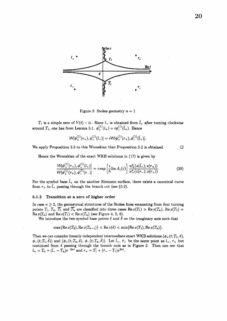
Figure 3: Stokes geometry $n=1$

$T_{1}$ is a simple zero of $V(t)-i\epsilon$ . Since $l_{\tau}$ is obtained from $l_{+}\mathrm{a}\mathrm{R}\mathrm{e}\mathrm{r}$ turning clockwisearound $T_{1}$ , one has from Lemma 5.1. $\phi_{\mathrm{Y}^{t}}^{(1)}(l_{+})=i\phi_{-}^{(1)}(l_{+})\wedge$ . Hence

$\mathcal{W}[\phi_{+}^{(1)}(r_{+}), \phi_{+}^{(1)}(l_{+})]=i\mathcal{W}[\phi_{+}^{(1)}(r_{+}\rangle,\phi_{-}^{(1)}(l_{+}^{\wedge})]$.We apply Proposition 3.3 to this Wronskian then Proposition 5.2 is obtained. $\square$

Hence the Wronskian of the exact WKB solutions in (17) is given by

$\frac{\mathcal{W}[\phi_{+}^{(1)}(r_{+}),\phi_{+}^{(1)}(l_{+})]}{\mathcal{W}[\phi_{+}^{(1)}(r_{+}),\phi_{-}^{(\overline{1})}(r_{-})]}=i\exp[\frac{i}{h}$im $A_{1}( \epsilon)],.\frac{w_{+}^{e}(z(l_{+}^{\wedge});z(r_{+}))}{u_{+}^{e}(\sim\sim(r_{-});z(r_{+}))}$ . (20)

For the symbol base $l_{+}^{\wedge}$ on the another Riemann surface, there exists a canonical curvefrom $\mathrm{r}_{+}$ to $l_{+}\wedge$ passing through the branch cut (see \S 5.2).

5.1.2 Transition at a zero of higher order

In case $n\geq 2$ , the geometrical structures of the Stokes lines emanating from four turningpoints $T_{1},$ $T_{n},$ $\overline{T_{1}}$ and $\overline{T_{n}}$ are classified into three cases ${\rm Re} z(T_{1})>{\rm Re} z(T_{n}),$ ${\rm Re} z(T_{1})=$

${\rm Re} z(T_{n})$ and ${\rm Re} z(T_{1})<{\rm Re} z(T_{n})$ (see Figure 4, 5, 6).We introduce the two symbol base points 6 and $\overline{\delta}$ on the imaginary axis such that

$\max\{{\rm Re} z(T_{2}), {\rm Re} z(T_{n-1})\}<{\rm Re} z(\delta)<\min\{{\rm Re} z(T_{1}), {\rm Re} z(T_{n})\}$ .

Then we can consider linearly independent intermediate exact WKB solutions $(\phi_{+}(t;T_{1}.\delta)$ ,$\phi_{-}(t;T_{1},\overline{\delta}))$ and $(\phi_{+}(t;T_{n},\delta),$ $\phi_{-}(t:T_{n},\overline{\delta}))$ . Let $\hat{l}_{+},\hat{r}_{+}$ be the same point as $\iota_{+},$

$r_{\mathrm{i}}$ butcontinued from 6 passing through the branch cuts as in Figure 2. Then one see that$\iota_{+}=T_{n}+(l_{+}^{\wedge}-T_{n})e^{-2\pi i}$ and $r_{+}=T_{1}+(\hat{r}_{+}-T_{1})e^{2\pi i}$ .

20

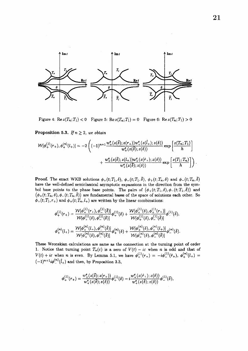
Figure 4: ${\rm Re} z(T_{n};T_{1})<0$ Figure 5: ${\rm Re} z(T_{n};T_{1})=0$ Figure 6: ${\rm Re} z(T_{n}; T_{1})>0$

Proposition 5.3. If $n\geq 2$ , we obtain

$\mathcal{W}[\phi_{+}^{(1)}(r_{+}), \phi_{+}^{(n)}(l_{+})]=-2((-1)^{n+1}\frac{w_{+}^{e}(z(\overline{\delta});z(r_{+}))w_{\tau}^{e}(z(l_{+}^{\wedge});z(\delta))}{w_{+}^{e}(z(\overline{\delta});z(\delta))}\exp[\frac{z(T_{n};T_{1})}{h}]$

$+, \frac{w_{+}^{e}(z(\overline{\delta});z(l_{+}))w_{+}^{e}(\sim\prime(\hat{r}_{\vdash}\rangle\}\tilde{\wedge}(\delta))}{u_{+}^{e}(z(\overline{\delta});z(\delta^{\neg}))}\exp[\frac{z(T_{1\backslash }T_{n})}{h}])$ .

Proof. The exact WKB solutions $\phi_{+}(t;T_{1}, \delta),$ $\phi_{-}(t;T_{1}.\overline{\delta}),$ $\phi_{+}(t\backslash T_{n}.\delta)$ and $\phi_{-}(t_{j}T_{n},\overline{\delta})$

have the well-defined semicl\"assical asymptotic expansions in the direction from the sym-bol base points to the phase base points. The pairs of $(\phi_{+}(t:T_{1}, \delta),$ $\phi_{-}(t;T_{1}.\overline{\delta}))$ and$(\phi_{+}(t;T_{n}, \delta),$ $\phi_{-}(t;T_{n},\overline{\delta}))$ are fundamental bases of the space of solutions each other. So$\phi_{+}(t;T_{1},r_{+})$ and $\phi_{+}(t;T_{n}, l_{+})$ are written by the linear combinations:

$\phi_{+}^{(1)}(r_{+})=\frac{\mathcal{W}[\phi_{+}^{(1)}(r_{+}),\phi_{-}^{(1)}(\delta)]}{\mathcal{W}[\phi_{\vdash}^{(1)}(\delta),\phi_{-}^{(1)}(\overline{\delta})]}\phi_{+}^{(1)}(\delta)+\frac{\mathcal{W}[\phi_{+}^{(1)}(\delta),\phi_{+}^{(1)}(r_{+})]}{\mathcal{W}[\phi_{+}^{(1)}(\delta),\phi_{-}^{(1)}(\overline{\delta})]}\phi_{-}^{(1)}(\overline{\delta})$,

$\phi_{+}^{(n)}(l_{+})=\frac{\mathcal{W}[\phi_{+}^{(n)}(l_{+}),\phi_{-}^{(n)}(\overline{\delta})]}{\mathcal{W}[\phi_{+}^{(n)}(\delta)_{!}\phi_{-}^{(n)}(\overline{\delta})]}\phi_{+}^{(n)}(\delta)+\frac{\mathcal{W}[\phi_{+}^{(n)}(\delta),\phi_{+}^{(n)}(l_{+})]}{\mathcal{W}[\phi_{+}^{(n)}(\delta)_{\backslash }\phi_{-}^{\langle n\rangle}(\overline{\delta})]}\phi_{-}^{(n)}(\overline{\delta})$.

These Wronskian calculations are same as the connection at the turning point of order1. Notice that turning point $T_{n}(\epsilon)$ is a zero of $V(t)$ –is when $n$ is odd and that of$V(t)+i\epsilon$ when $n$ is even. By Lemma 5.1, we have $\phi_{+}^{(1)}(r_{+})=-i\phi_{-}^{(1)}(\hat{r}_{+}),$ $\phi_{+}^{(n)}(l_{+})=$

$(-1)^{n+1}i\phi_{-}^{(n)}(l_{+})\wedge$ and then, by Proposition 3.3,

$\phi_{+}^{(1)}(r_{+})=’\frac{u_{+}^{e}(z(\overline{\delta}):z(r_{+}))}{w_{+}^{\rho}\prime(z(\delta);z(\delta))}\phi_{+}^{(1)}(\delta)-i\frac{u_{+}^{e}1(z(\hat{r}_{\mathit{1}})_{\backslash }z(\delta))}{w_{+}^{e}(\wedge(\sim\overline{\delta});\sim(r\delta))}.\phi_{-}^{(1)}(\overline{\delta})$ .

21

$\phi_{+}^{(n)}(l_{+})=,\frac{w_{+}^{e}(z(\overline{\delta});z(l_{+}))}{u_{+}^{e}(z(\overline{\delta});z(\delta))}\phi_{+}^{(n)}(\delta)+(-1)^{n+1}i’\frac{u_{+}^{e}(z(l_{+}^{\wedge});z(\tilde{\delta}))}{w_{+}^{\mathrm{e}}(z(\overline{\delta});z(\delta))}\phi_{-}^{(n)}(\overline{\delta})$,

$= \frac{w_{+}^{e}(z(\overline{\delta});z(l_{+}))}{w_{+}^{e}(z(\overline{\delta});z(\delta))}e^{z(T_{1;}T_{n})/h}’\phi_{+}^{(1)}(\delta)+(-1)^{n+1}i.\frac{w_{+}^{e}(r(l_{+}^{\wedge}))\sim\prime(\delta)\rangle}{w_{+}^{e}(z(\overline{\delta});z(\delta))}e^{z(T_{n_{)}}\cdot T_{1})/h}\phi_{-}^{(1)}(\overline{\delta})$ .

From these relations, we have Proposition 5.3.$\square$

Applying Proposition 5.3, we have

$\frac{\mathcal{W}[\phi_{+}^{(1)}(r_{+}),\phi_{+}^{(n)}(l_{+})]}{\mathcal{W}[\phi_{+}^{(1)}(r_{+}),\phi_{-}^{(\overline{1})}(r_{-})]}=i\exp[-\frac{i}{2h}(\overline{A_{1}(\epsilon)}+A_{n}(\epsilon))]\frac{1}{w_{+}^{e}(z(r_{-});z(r_{+}\rangle)}$

$\mathrm{x}((-1)^{n+1}\frac{w_{+}^{e}(z(\overline{\delta});z(r_{+}))w_{+}^{e}(z(l_{+}^{\wedge});z(\delta))}{w_{+}^{e}(z(\mathit{5});z(\delta))}\exp[\frac{i}{h}A_{n}(\epsilon\rangle]$

$+ \frac{w_{+}^{e}(z(\hat{\delta});z(l_{+}))w_{\perp}^{e}(z(\hat{r}_{+}):z(\delta))}{w_{+}^{e}(z(\overline{\delta});z(\delta))}\exp[\frac{i}{h}A_{1}(\epsilon)])$ (21)

Note that there exists a canonical curve for each Wronskian calculation (see \S 5.2).

5.2 Asymptotics of the Wronskians as $harrow \mathrm{O}$

About the calculations of the asymptotic expansions of the Wronskian (19), $(20\rangle,$(21) as$harrow \mathrm{O}$ , we must pay attention to the distance between the canonical curve and the turningpoints on the complex $z$-plane because $z=z(T_{j})$ are simple poles of $H’(z)/H(z)$ . We givethe figures of the canonical curve on the complex $z$-plane, where the phase base point isequal to $0$ .

For the Wronskian in (19), the canonical curve from $z(r_{+})$ to $z(l_{-})$ passes between$z(T_{1})$ and $z(\overline{T_{1}})$ as in Figure 7. Therefore we get

$w_{+}^{\mathrm{e}}(z(l_{-});z( \mathrm{r}_{+}))=1+O(\frac{h}{{\rm Re} z(\overline{T_{1}})-{\rm Re}_{\tilde{k}}(T_{1})})$ as $harrow 0$ .

By Lemma 2.1, we have

${\rm Re} z(\overline{T_{1}})-{\rm Re} z(T_{1})=O(\epsilon^{\underline{n}\pm\underline{1}}n)$ as $\epsilonarrow 0$ .

In case $n=1$ , for the Wronskian in (20), the canonical curve from $z(r_{+})$ to $z(l_{+})\wedge$

through the branch cut passes over $z(T_{1})$ as in Figure 8.

$w_{+}^{e}(z(l_{+}^{\wedge});z(r_{+}))=1+O(h)$ as $harrow 0$ .

Therefore we obtain, in case n— 1,

P$($ \^e, $h)= \exp[-\frac{2}{h}{\rm Im} A_{1}(rightarrow)\overline{\vee}](1+O(h\rangle)$ as $harrow$. $0$ .

22

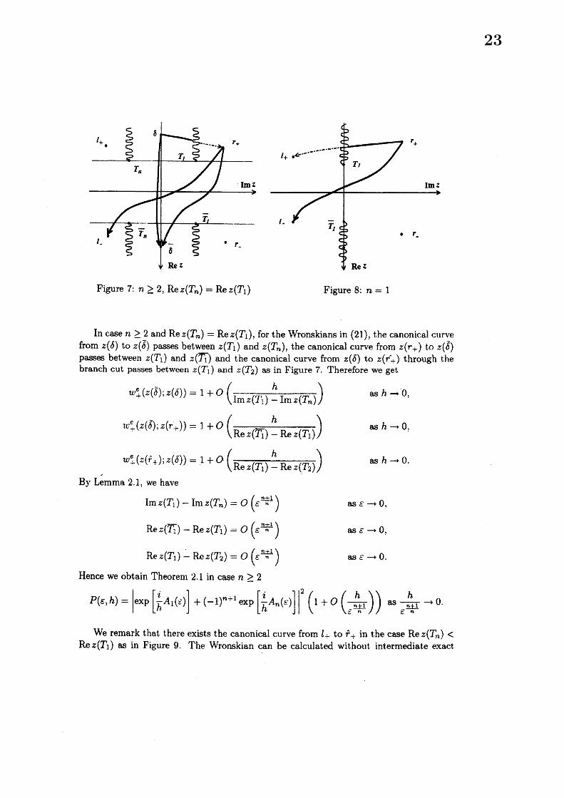
Figure 7: $n\geq 2,$ ${\rm Re} z(T_{n})=\mathrm{R}\epsilon z(T_{1})$ Figure 8: $n=1$

In case $n\geq 2$ and ${\rm Re} z(T_{n})={\rm Re} z(T_{1})$ , for the Wronskians in (21), the canonical curvefrom $z(\delta)$ to $z(\overline{\delta}\rangle$ passes between $z(T_{1})$ and $z(T_{n})$ , the canonical curve from $z(r_{+})$ to $z(\overline{\delta})$

passes between $\sim \mathit{7}(T_{1})$ and $z(T_{1^{-}})$ and the canonical curve from $z(\delta)$ to $\approx(r_{+}^{\wedge})$ through thebranch cut passes between $z(T_{1})$ and $z(T_{2})$ as in Figure 7. Therefore we get

$u_{+}^{e}’(z( \hat{\delta});z(\delta))=1+O(\frac{h}{{\rm Im} z(T_{1})-{\rm Im} z(T_{n})})$ as $harrow 0$ ,

$\iota\iota_{+}^{e}.(z(\delta);z(r_{+}))=1+O(\frac{h}{{\rm Re}_{\wedge}^{\sim}(\overline{T_{1}})-{\rm Re} z(T_{1})})$ as $harrow 0$ ,

$u_{+}^{e}’(x( \hat{r}_{+});z(\delta))=1+O(\frac{h}{{\rm Re} z(T_{1})-{\rm Re}_{\sim}(T_{2})},)$ as $harrow 0$ .

By Lemma 2.1, we have

${\rm Im}\approx(T_{1})-{\rm Im} z(T_{n})=O(\epsilon^{\frac{\mathfrak{n}+1}{n}})$ as $\epsilonarrow 0$ ,

${\rm Re}\approx(\overline{T_{1}})-{\rm Re} z(T_{1})=O(\epsilon^{\frac{n+1}{n}})$ as $\epsilonarrow 0$ ,

${\rm Re} z(T_{1})-{\rm Re} z(T_{2})=O(\epsilon^{\frac{n+1}{n}})$ as $\epsilonarrow 0$ .

Hence we obtain Theorem 2.1 in case $n\geq 2$

$P( \epsilon,h)=|\exp[\frac{i}{h}A_{1}(\epsilon)]+(-1)^{n+1}\exp[\frac{i}{h}A_{n}(\epsilon)]|^{2}(1+O(\frac{h}{\vee^{\frac{n+1}{n}}=}))$ as $\frac{h}{\epsilon^{\frac{n+1}{n}}}arrow 0$ .

We remark that there exists the canonical curve from $l_{+}$ to $\hat{r}_{+}$ in the case ${\rm Re} z\langle T_{n})<$

${\rm Re} z(T_{1})$ as in Figure 9. The Wronskian can be calculated without interm\’eiate exact

23

WKB solutions as follows:

$\mathcal{W}[\phi_{+}^{(1)}(r_{+}), \phi_{+}^{(n)}(l_{+})]=\exp[\frac{i}{2h}(A_{1}(\epsilon)-A_{n}(\epsilon))]\mathcal{W}[\phi_{+}^{(1)}(r_{+}), \phi_{+}^{(1)}(l_{+})]$ ,

$=-i \exp[\frac{i}{2h}(A_{1}(\epsilon)-A_{n}(\epsilon))]w_{+}^{e}(\approx(\hat{r}_{+});z(l_{+}\rangle)$ .

$w_{+}^{e}(z( \hat{r}_{+});z(l_{+}))=1+O(\frac{h}{{\rm Re} z(T_{1})-{\rm Re} z(T_{n})})$ as $harrow 0$ .

By Lemma 2.1, we have

${\rm Re} z(T_{1})-{\rm Re} z(T_{n})=O(\epsilon^{(n+2m)/n})$ as $\epsilonarrow 0$ .

The asymptotic expansions (6), (5) in Proposition 2.1 imply that $P(\epsilon, h)$ in case $n\geq 2$

can be calculated as in case $n=1$ when $h$ goes to $0$ faster than $\epsilon^{(n+2m)/n}$ tends to $0$ (seeFigure 4).

Figure 9: $n\geq 2,$ ${\rm Re} z(T_{n})<{\rm Re} z(T_{1}\rangle$

References[AKT] T. Aoki, T. Kawai and Y. Takei: Exact WKB analysis of non.-adiabatic transition

probabilities for three levels, J. Phys. A: Math. Gen. 35 (2002), 2401-2430

[BM] H. Baklouti and M. Mnif: Asymptotique des r\’esonances pour une barri\‘ere de poten-tial d\v{c}g\’en\’er\’ee, preprint

[BT] V. Betz and S. Teufel: Landau-Zener formulae from adiabatic transition histories,preprint

[CLP] Y. Colin de Verdi\‘ere, M. Lombardif and J.Poll\"et: The microlocal $Land_{\text{ノ}}au$-Zenerfor.mula, Annales de I’I.H.P. Physique Th\’eorique 71, 1 (1999), 95-127

24

[FLN] S. Fujii\’e, C. Lasser and L. Nedelec: Semiclassical resonances for a two-levelSchr\"odinger operator with a conical intersection, preprint

[FR] S. Fujii\’e, and T. Ramond: Matrice de scattering et r\’esonances associ\’ees a’ une orbiteh\’et\’erocline, Annales de I’I.H.P. Physique Th\’eorique 69, 1 (1998), 31-82

[GG] C. G\’erard and A. Grigis: Precise estimates of tunneling and eigenvdues near apotential barrier, J. Diff. Equations 42 (1988), 149-177

[H] Hagedorn G. A.: Proof of the Landau-Zener formula in an adiabatic limit with smalleigenvalue gaps, Commun. Math. Phys. 136, 4 (1991), 33-49

[HJ] Hagedorn G. A. and A. Joye: Recent results on non-adiabatic transitions in Quan-tum m,echanics., Proceedings of the 2005 UAB International Conference on Differen-tial Equations and Mathematical Physics, Birmingham, Alabama. March 29-April 2(2005)

[J1] A. Joye: Non-Tbtvial Prefactors in Adiabatic Transition Probabilities Induced by High-Order degeneracies, J. Phys. A 26 (1993), 6517-6540

[J2] A. Joye: Proof of the Landau-Zener formula, Asymptotic Analysis 9 (1994), 209-258

[JKP] A. Joye, H. Kunz and C.-E. Pfister: Exponential Decay and Geom.et,ric Aspect ofTransition Probabilities in the Adiabatic Limit, Ann. Phys. 208 (1991), 299-332

[JP1] A. Joye and C.-E. Pfister: Semiclassical Asymptotics Beyond all Orders for Simple$Scatte;\dot{\tau}ng$ Systems, SIAM J. Math. Anal. 26 (1995), 944-977

[L] L. D. Landau: Collected Papers of L.D.Landau, Pergamon Press (1965)

[M] A. Martinez: Precise exponential estimates in adiabatic theory, J. Math. Phys. 35(1994), 3889-3915

[Ra] T. Ramond: Semidassical study of Quantum scattering on the line, Commun. Math.Phys. 177 (1996), 221-254

[Ro] V. Rousse: Landau-Zener transitions for eigenvalue avoided crossing in the adiabattcand $Bom$-Oppenheimer approanmations, Asymptot. Anal. 37 (2004): no. 3-4, 293-328

[T] S. Teufel: Adiabatic Perturbation Theory in Quantum Dynamics. Springer LectureNotes in Mathematics 1821 (2003)

[W] T. Watanabe: Adiabatic transition probability for a tangential crossing. preprint

[Z] C. Zener: Non-adiabatic crossing of energy levels: Proc. Roy. Soc. London 137 (1932),696702

[ZN] C. Zhu and H. Nakamura: Stokes constants for a certain dass of second-order ordi-nary differential equations, J. Math. Phys. 33 (1992), 2697-2717

25