RIGHT:

URL:

CITATION:

AUTHOR(S):

ISSUE DATE:

TITLE:

Diffraction of Seismic SH WavesCaused by the Earth's Core

SAKAI, Akio

SAKAI, Akio. Diffraction of Seismic SH Waves Caused by the Earth'sCore. Bulletin of the Disaster Prevention Research Institute 1974, 24(2):81-105

1974-06

http://hdl.handle.net/2433/124842

Bull. Disas. Prey. Res. Inst., Kyoto Univ., Vol. 24, Part 2, No. 220, June, 1974 81

Diffraction of Seismic SH Waves Caused by the Earth's Core

By Akio SAKAI

(Manuscript received June 29, 1974)

Abstract

The amplitude decay function of diffracted SH waves caused by the earth's core near the geometrical shadow point is explicitly derived from the Kelvin's stationary phase method with

inhomogeneity parameters. Seismic SH waves from six intermediate and deep earthquakes are Fourier analysed by selecting

suitable stations in the epicentral distances beyond 90 degrees. We empirically introduced the amplitude decay r from the observed trend of the relation between distances and logarithmic

amplitude spectra of the SH component. It is verified that the amplitude decay function is appropriate for interpreting r in the first order. It is also suggested that a low velocity layer and

lateral inhomogeneities might exist at the base of the mantle.

1. Introduction

Much work has been done on the velocity structure of the interface between the earth's core and the mantle from the beginning of this century by a number of in-vestigators such as Wiechert", Gutenberg'', Jeffreys'', Dahm4', Lehmanns' and others. Their immediate purpose was to provide or improve travel time tables for seismic waves of P, S, PcP, ScS and other types. These researches have produced stimulating results. But closer investigations must still be concentrated on singular

points of the travel time curves which are associated with discontinuities of the velocity structure, such as the core-mantle interface, since the method taken so far was restricted principally to the time-domain.

Through progress in the wave form analysis (Fourier transform) by the aid of an

electronic computer, the attention of the seismologist is attracted to the "frequency dependence of travel time curves", particularly of diffracted waves caused by the earth's core. This type of research became possible through development of theory and research techniques. There are now a number of observational data of teleseismic body waves and some results from experiments on wave transmission by Rykunov61,

Sacks'', Alexander and Phinneys', Teng and We, Teng'°', and Shimamuraw. The present author intends to study seismic disturbances caused by a cylinder

which is a model of the earth's core, and furthermore, to provide a theoretical basis for elucidating the velocity structure of the core-mantle interface by using diffracted SH waves. As is well known, by using the SH mode we make the equations of motion and boundary conditions degenerative. We also present the observational data adequate to Fourier transform and calculate an apparent attenuation function r

near the geometrical shadow point.

82 A. SAKAI

2. Theoretical Formulation

a. Histrical Review and Some Comments

We must pay careful attention to the study of the diffraction phenomena in optics and accoustics, since their mathemetical treatment is generally the same whenever we are dealing with waves disturbed by a spherical or cylindrical body.

Historically a scattering law of Rayleigh'2' is the first solution to the problem established under the assumption that the product of the wave number and the dimension of the obstacle is very small. The high frequency scattering problem is

partly solved by using analytical approximation method by Watson's', van der Pol and Bremmer14', Rubinow and Keller's', Nussenzweig16', Duwalo and Jocobsn' et al., and numerically on an electronic computer by Phinney and Alexander's', Phinney and Cathles19), sato20)21', Chapman and Phinney22' et al.

We may group them according to mathematical formulation. One is a "direct" summing, which is the so-called partial wave expansion, and the other is an "integral

transformed" summing, which is derived from the so-called Watson's transformation or Poisson's summation formula. The former has revived at the age of electronic computers, but we cannot 'know the change of the results when certain alternation of each parameter may take place. The latter has some limitations in the approximation of the Hankel function, but by paying careful attention to the conditions of the fre-

quencies, the dimensions of the obstacle and the observation points, we can obtain a direct representation of the principal part of the solution.

b. Condition and Formalism

The amplitude field disturbed by a sphere or a cylinder is divided into some regions characterized by the frequencies and the dimensions of the obstacle, say, a Fresnel region, a transition and a deep shadow region (Nussenzweig)16'. The analysis so far made using seismic body wave data to infer the structure of the core-mantle interface was based on the fact that the first pole of a reflection coefficient is a structure-sensitive

parameter (Phinney and Alexander)m. Their results; however, are incomplete or impractical on the handling of seismic body wave data, because the long-period seismograms (T1=1.5-30 sec, T2=90--100 sec) obtained at the WWSSN (world-wide standardized station network) are inadequate to the wave form analysis, even if a most appropriate seismic event is selected in a sense of the magnitude and the observed SN ratio at each station, far beyond one hundred degrees. This is one reason why this field of research is difficult. In accordance with demands on practical observations stated above, the behavior of wave amplitudes in the region of transition i.e., near one hundred degrees, must be discussed fully.

The factors affecting the amplitude function may be as follows.

(A) Modes of the oscillation (SH or P–SV type) (B) Boundary conditions

(C) Energy dissipation in the medium : departure from perfect elasticity

Diffraction of Seismic SH Waves Caused by the Earth's Core 83

(D) Observation point and frequency response of observation apparatus Although point (C) is the most important information on the present physicochemical

state and moreover on evolution of the earth, our knowledge about theories and experiments on anelasticity under the condition of conjectured temperature and

pressure is awfully poor. A mathematical formulation is now impossible; thus an effect such as anelasticity is left pendent. It is to be noted, however, that there are some studies of Shimamura"), Tenglo, and Mikumo and Kurita23' which assume

Q-type (frequency independent) dissipation models. Let's investigate points (B) and (D). We assume that a plane SH wave is incident

on a cylindrical cavity whose line of symmetry is parallel to wave front and to the direction of oscillation. We set the cylindrical coordinates simultaneously centered

by the line of symmetry of a cylindrical cavity and an observation point as (r,0). It is easily proved that a scattered wave will be of the same type as the incident wave and

that the boundary is stress free if the rigidity in the cavity is neglected, whenever an incident wave is of the SH type.

( r ,e)

cavity mod e 1.1

SH waves Fig. I Scattering geometry for an incident wave and an observer in cylindrical

coordinates (r,O,z). All of the quantities are not functions of z and the direction of the oscillations is restricted to that of z, where b is the radius of the cavity (Model 1)

When we expels an incident wave as U, = exp(i Icor cos 0) (1) and a scattered wave as U,

(for brevity we neglect the term exp(—hot)), we easily get the Neumann expansion or more popularly the partial wave expansion,

exp(i Icor cos@) = (kor)exp [i (a + 2ni(2) where k. is the wave number of an incident wave and b istheradius of a cylindrical

cavity. Applying the asymptotic expansion of the Hankel function H„")(p) and H,'2' (p) when the variable p tends to infinity, we may have conditions necessary for 11

a scattered wave U,'"'2— C„1-1."' (k.r) and for an incident wave U,("1——2 H„(2)

(kJ) (providing that U,'"' and Us") is the n-th term concerning the variable r) Then we have,

–

U5 =1—E [H„(2) (Icor) C, Ha") (kJ)] exp [i (61+2(3) 2 n=-0.

84 A. SAKAI

C. will be determined by boundary conditions including a cylindrical layered structure at the interface. Later we will show the relation C_„ = exp(—i 27r n) C,, in the assumed models. Consequently utilizing Poisson's summation formula,

E co (n) (r) exp ( — i27rvr) dr (4) -co

-r7r Uz =1—Eexp [i (-2 + B + 2nm) r] 1.11,(2) (kJ) + CJI,") (kor)] dr 2 .,0

exp [i2— 0 + 2nm)r] [14(2) (kor)CJI,(1)(kor)idri (5) If contributions to the integral ofthe integral function near infinity on the r-plane

can be neglected (actually we have already assumed the above condition in deriving the above relation (4)), Cauchy's theorem in complex calculus is applicable with the

path of integration transformed into the loop (See Fig. 2). The above stated fact can be demonstrated in the case of Model I defined so that the medium of the mantle is uniform. The outline of demonstration is based on the fact that the Hankel function shows a different approximate behavior in the domains split by the anti-Stokes lines, the real axis and imaginary axis. On the other hand, the poles of the function C,

(reflection coefficient) of the variable r reside on the first quadrant, in case of a sphere, which has been shown"). Hence we suppose that the principal term of Uz is

1 Uz—2 [f exp [i 2— 0)r]CH:" (k or) dr R limy

exp [i (-172+ 0) r] C, H,"(k or) dr] (6) R „

on the condition that 0 < 0 < 2

"C- Plane

411

0

Fig. 2 The path of integration transformed into the upper half-plane and real axis where the dotted lines represent anti-Stokes lines of Hankel function

in the first quadrant ($=kob, p=kor)

Diffraction of Seismic SH Waves Caused by the Earth's Core 85

The remnant terms may be interpreted physically as creeping waves contributed by poles of Cr (See Fig. 3)

Fig. 3 Homeomorphic-transformed creeping waves which encircle the cylindrical cavity repeatelly and decay exponentially in an order of exp(---$34 x path

length)

Next we shall estimate the above obtained function U: analytically near the

shadow point 80 = sin-1 —6 In the first place, under the same assumption as neglect-

ing contributions from the so-called creeping waves, we may neglect the second term. Now replacing Icab by

rd andIcor by p (6) can be rewritten as, 21./, ffexp[i(-27r— 0)r]CA") (p)dr

f exp [i (-2— 0)r] (Cr-1) H,") (p)dr

±rexp [i 2— 0)r] H1(,)(p) dr (7)

The division into three terms is performed with the intention of getting analytical expressions separately ; the terms related to the dimensions of the obstacle (the radius of the cylinder) and the boundary condition of Model 1 or of more general models, and a non-related term which does not include the term of a reflection coefficient. The asymptotic behaviors of Cr change from the oscillatory ones to the convergent ones with passing through the point 8 on the real axis. As for the behavior of 1-1,'"(p) it is oscillatory if the path of integration is restricted to the left of the anti-Stokes line on the first quadrant. If I r p is comparable with I r Ix, the expansion of 14")(p) and

11,")(p) is expressed by the Airy function Ai(*) by which computations at the neigh-bourhood of the shadow point r=3 will be performed with using the Debye's expan-sion of 14")(p) for lr <p under the conditions stated below.

With regard to the third term, we use the first term of the Debye's asymptotic expansion of the Hankel functions" 11,:u (p)

86 A. SA X.41

When iri < p and Iv— pl >11"A

I,")(p).-- (p2—r2)-X exp i [(p2 z-934 — rcos-1 —p — —4] (8) Hence Integrand (-2 )}1 (p2—r2)-)( exp i [r (sin-l— — + (02 —1.2)34 —

4

(9)

With sine substituted for -- , the method of stationary phase is applicable. From

the expression of partial derivative of f(co) =69-0) psinvpcosv—-7-4 with respect to co, the saddle point 9=0.

Including higher derivatives,

1 f(co) pcos0 —4 +2 —1 °cos°—3— 0)2 — psin0—+ (10)

re 9-nxpL-pcoso (the 3rd term) (2 pcos0 )Kexp (i pcose i4)2— 0)2] do r=0

(I I)

where rpm corresponds to infinite point in the expression (7), noticing the condition

for neglecting the higher order term, ({0 — (03 psin0 << 1. (12)

Because the principal contribution to the integral of the integrand resides in the neighbourhood of the saddle point, we may replace rpm for infinity in this case. For later convienience the half of the 3rd term is transformed as,

1- l'exp (i (62) dm x exp (1 pcos0 — i —4) (13)

where 0, = sin-1 —r and v = (pco2s0 )x (0-0a) With regard to the 1st and 2nd terms, we use the expansion as in the first case for

11;1'(p) and the asymptotic expansion for the function Cr on the conditions r and <

(2pcose)54 exp pcos04i7r) [.1.6°C2 .exp [ipops° (yo— 0)2]4 ri ocosoor]d co](14)

as

— 1) exp L

If we replace (1)x p(sinv — sinea) by X

(-82 )1/2 (0 — 0) by Y and (A,2Azpeoscor,, by Z

Diffraction of Seismic SH Waves Caused by the Earth's Core 87

then

(the 1st + the 2nd term) — ( irpco2sy7)M exp (i pcos0 —i 42i 2) (11)M • (const) (15)

where

(const) — C exp (i Z2X2 iXY)dX (C-1) exp (i Z2X2 iXY)dX (16)

0

Adding the terms evaluated analytically, we have reached the expression of the

amplitude in the neighbourhood of the shadow point with inhomogeneity parameters

included implicitly in the function C,

(i1))4 • const 7t 1( 2irPCOSO-)342 exp (i pcos0 — i4) [ 2 exp 4 (00-0) + (27rpcos0)x

(17)

In the case of Model 1. calculated results of "const" are, in numerical integration under the assumption that Y and Z is neglected with the expansions of

11,.")($) = 2 exp (i3)(r2 )}� AlAi (exp (2 )m—713)) (18) H(2)(6) = 2 exp (— 3)(r—)S Ai (exp (—3)(irr(r —B))

r U

for the condition thatOr= 0 at r = b, const = —0.55-0.95 1 (19) and for the

condition that Li, = 0 at r b (rigid core) const = 0.64 + 1.10 i (20) which show

good agreement with the analytical calculations based on a somewhat different formulation from ours 25'26' For computations the Hankel function of the 3rd order

is used as the following forms.27)

Z < 0 Ai(Z) = —1 23Z(-- [ef; Hs") (C)e-tr -K(2)(C)]

Ai(a. Ze17) = Leif (— Z314�"}(C) (21)

Z> 0 Ai(Z)= 2(Z3)31 e* He)(Ces.)

Ai(Zea3xe = — - Z 23YEetHx'" (Cet;)

3

where C = ( 3-/1ZT These results suggest the rigidity in the core has significant effects on the determi-

88 A. SAKAI

nation of the core radius even with the aid of scalar waves i.e., SH waves. If the ri-

gidity in the core is negligibly small, we should estimate a radius of the core much smaller from the amplitudes decay of seismic waves. Hence it must be useful for the determination of the core radius, the core rigidity and stress conditions at

the interface to estimate the shadow point from the amplitude spectra of rather high frequencies with taking care of frequency dependence of the shadow point expressed

by (17). Although it has not yet been fully established, we may incidentally mention

that the amplitudes just near the shadow point would depend only on the local curvature of the scatterer, for example, a cylinder, a sphere, an ellipsoid and a

paraboloid. It will be studied explicitly in near future.

c. Recurrence Formula for Layered Models

In this section we shall introduce a layered model as a representative of inhomo-

geneity to obtain a functional form of C, The equation of motion is obtained by adding forces

2

Dt 2 U. — (O ± 1 )r z+ r 001a OzOzzz (22)

r

rz, Oz and zz being the Eulerian stress tensor which can be replaced by

Uz 1 OU.prz =az r 00 Or-/Iand zz — (A + 2p) azUz (23)

where p is the density and it the rigidity of the elastic media. If we suppose that

D2/Dt2 cr#.0210t2, Olaz 0, p = constant, Uz is proportional to exp (inc —hot). For simplicity Uz is substituted for a function of the variable r,

d dU, p d n2 drdrr dr

U z(pm' — r2g) Ur = 0 (24) where /2 is an integer.

We can rewrite it as follows,

1n'

d (U1) owz(1_k2r2u dr k U2 1

0 (U2)(25)

U, = u dr11. , U2 = Ur

where k = colA and 82 pip This is a well-known second order differential equation system. Although there are

many methods for solving this system, say the Runge-Kutta interpolation method, for the time being we are not relying on that method. For the solution can be re-

presented by the Hankel function, in case p(r) is proportional to the power of Y.

Diffraction of Seismic SH Waves Caused by the Earth's Core 89

core

interface mantle

Fig. 4 Model A composed of a uniform mantle and a layer with the rigidity continously varied

We introduce Model A as given below,

= 0 r <b

= ao(r1102° b < r <ri (a> —1) (26)

= it0 < r

The equation (24) under the structure (26) is easily resolved in the form

1 U. cc—2 {H,(2) (kJ) + C„Hn") (kor)} r> r1

U. cc —1IilfiraH„(2)(Z)Bnralt(" (Z)) b < r <1'1 2

where kn,11and Z are expressed bya) N b,(a2+122)HI(n+ 1) anda+J'1(r)a+1 respectively. A„ is the amplitude of the n-th partial wave in the interface between

the uppermost layer and the cavity which descends to the cavity, B, is the one which ascends to the uppermost layer and C, is the one which ascends to the observation

point. The conditions for the continuity of the displacements and the stresses at each of interfaces and for the stress free at the base of the mantle yield A„, B„ and

C. as functions of the variable r. An, B, and C, for a more general multi-layered model will easily be derived by the matrix-product formalism.28)

It should be reminded here that we have to demonstrate supplementary relations.

To establish C., = exp (—i2nt) C, we make use of the relations

H(1)(Z)= exp (kit) H,'"(z) and H_,)2)(Z)= exp (— kr) Hr(2)(Z) (27)

The Wronskian of Hr(1)(Z) and H,(2)(Z) for inversion of the matrix are necessarily used. The final product of matrices is

(C., 1) = K (aims, alb)

where K is the complex constant. As C. is the amplitude of the n-th partial wave in the uppermost layer of the general model, the total wave amplitude is proportional

90 A. SAKAI

to H,,(2' (kor)± C„.11„") (kor) with respect to the radial parameter. If we select

J„(Z) and Y.(Z) for the general solution of the wave equation, the final matrix pro-duct will be (C, + 1, i (C. — I)) = K' (a,' D',a2' D') As far as the parameter n is a real number, the absolute value of C. is equal to unity. This result is helpful for the application of the method of stationary phase to general models.

3. Observation Data

a. Data and Assumptions

The long-period seismograms recorded at stations of the WWSSN are analysed

by the Fourier transform method, in the distance range beyond ninety degrees, which corresponds to the region of interference between incident and scattered waves. From the Fourier spectra of the NS and EW components, SH component is derived by the transformation of the Cartesian coordinates. Local station effects which

possibly alter the direction of oscillation are not taken into consideration here, because the crustal structure beneath the stations are still open to argument.

Things relevant to the analysis such as window techniques and aliasing are referred to Blackman and Tukey (1959)29) and Goldman (1953)°1. The adopted time window, the truncated length for seismic phase and digitized interval are

W(1)= 0.54 + 0.46 cos (rtIT)

T = 30 sec 60 sec (28)

dt = 0.5 sec — 1.2 sec

respectively. We have selected stations in almost the same azimuth seen from the epicenter to minimize possible differences in the spectral structure of the waves radiated from the source. We also assumed that the structure in the neighbouhood of the source is almost uniform and that effects of the crust and upper mantle due to lateral inhomo-

geneity is negligible. The presumed linear response system of the SH component will be written

as follows;

aPo(w)—> PM, (w) —> PM CB (W) P M 2(0) P (CO

where a is the spatial term and Po(w) the frequency dependent term due to the source time function, Pm,(0) the frequency response along a ray path from a source down to the base of the mantle, PAIC BM the response of a diffracted wave or a ray grazing the earth's core, PM2(0) the response along a ray path from the base of the mantle up to the earth's surface and 131(o)) the response of an apparatus. When the corrected amplitude at the i-th station by terms of a, Po(o) and Pt(w) is expressed as Mao) and PmcB(0)) at the i-th station as /12,„(0)),

Diffraction of Seismic SitWaves Caused by the Earth's Core 91

P an(60) A g),-(10) (29)

nc,3(0) AVA04

The above stated circumstances are diagrammed simply in Fig. 5.

mantle

source

c ore

Fig. 5 A diagram of rays grazing along the base of the mantle: we assume that the distortion of the amplitude and phase spectra is attributed to the structure near the core-mantle interface except the effects of the source

spectra of each direction.

The adopted criteria of selecting seismic events for executing the wave form analysis

are to restrict ourselves to the focal depths greater than 100 km in order to isolate the diffracted S waves from adjacent phases, such as SKS, SKKS, pS or SP, to a range of magnitudes to avoid contamination by other phases and to suitable regions of the epicenters subject to present distribution of stations of the WWSSN with the spatial term of radiation taken into consideration.

We also refer to Katsumata and Sykes (1970)3", Fitch and Molnar (1970)32', 'sacks and Molnar (1971)33' and others34'35' in selecting suitable seismic event, of

which parameters together with information on relevant stations are listed in Table I and 2. The radiation pattern of P wave first motions projected on a Wulf net and contours of a seismic zone near the source are reproduced from their papers with

Table I Data of the earthquakes and referred papers

EventOrigin Time Epicenter Depth Magnitude Referred Paper (GMT)

No. 1 1968 May 14 29.93" 129.37E 168 km 5.9 Mikumo (1971)) 14" 5m 6.048

No. 4 1965 Sept 21 28.96" 128.23E 195 6.0 Katsumata and lh 38m 30.38 Sykes (1969)30

No. 5 1963 May I 19.0" 168.9E 142 6.8 Isacks and 1.0h 3m 20.08 Molnar (1971)331

No. 6 1965 Aug 20 5.74" 128.63E 328 6.1 Fitch and 5h 54m 50.68 Molnar (1970)14

No. 7 1967 May 21 0.97" 101.47E 173 6.3 Fitch and 18h 45m 11.7a Molnar (1970)341

No. 8 1966 Mar 17 21.08" 179.18' 626 6.2 Isacks, Sykes 15h 50m 32.28 and Oliver (1969)34'

92 A. SAKAI

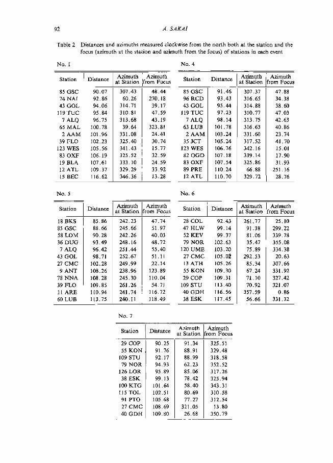
Table 2 Distances and azimuths measured clockwise from the north both at the station and the focus (azimuth at the station and azimuth from the focus) of stations in each event

No. 1 No. 4

Azimuth Azimuth Azimuth Azimuth Station DistanceStation Distance at Station from Focusat Station from Focus

85 GSC 90.07 307.43 48.44 85 GSC 91.46 307.37 47.88 74 NAL 92.86 60.26 270.18 96 RCD 93.43 316.65 34.38 43 GOL 94.06 314.71 39.17 43 GOL 95.44 314.88 38.60 119 TUC 95.84 310.81 47.59 119 TUC 97.23 310.77 47.03 7 ALQ 96.75 313.68 43.19 7 ALQ 98.14 313.75 42.63 65 MAL 100.78 39.64 323.81 63 LUB 101.78 316.63 40.86 2 AAM 101.96 331.08 24.41 2 AAM 103.24 331.60 23.74 39 FLO 102.23 325.40 30.74 35 JCT 105,24 317.52 41.70 123 WES 105.56 341.43 15.77 123 WES 106.76 342.16 15.01 83 OXF 106.19 325.52 32.59 82 OGD 107.18 339.14 17.90 19 BLA 107.61 333.10 24.59 83 OXF 107.54 325.86 31.93 12 ATL 109.37 329.29 33.92 89 PRE 110.24 66.88 251.16

15 BEC 116.62 346.36 13.28 12 ATL 110.70 329.72 28.76

No. 5 No. 6

Station Distance Azimuth AzimuthStation DistanceAzimuth Azimuth at Station from Focusat Station from Focus

18 131(5 85.86 242.23 47.74 28 COL 92.43 261.77 25.10 85 GSC 88.66 245.66 51.97 47 HLW 99.14 91.38 299.22

58 LOM 90.28 242.26 40.03 52 KEV 99.37 81.06 339.78 36 DUG 93.49 248.16 48.72 79 NOR 102.63 35.47 355.08 7 ALQ 96.42 251.44 55.40 120 UME 103.20 75.89 334.38 43 GOL 98.71 252.67 51.11 27 CMC 105.02 292.53 20.63 27 CMC 102.28 249.99 22.14 13 ATH 105.26 85.34 307.66

9 ANT 108.26 238.96 123.89 55 KON 109.30 67.24 331.92 78 NNA 108.28 245.30 110.04 29 COP 109.31 71.10 327.42 39 FLO 109.85 261.26 i 54.71 109 STU 113.40 70.92 321.07 11 ARE 110.94 241.74 116.72 40 GDH 116.56 357.59 0.86

60 LUB 113.75 240.11 118.49 38 ESK 117.45 56.66 331.32

No. 7

Azimuth Azimuth Station Distanceat Station from Focus

29 COP 90.25 91.34 325.51 55 KON J 91.76 88.91 329.48 109 STU 92,17 88.99 318.58 79 NOR 94.93 62.23 352.52 126 LOR 95.89 85.06 317.26 38 ESK 99.13 78.42 325.94 100 KTG 101.64 58.40 343.31 115 TOL 102.51 80.69 310.58 91 PTO 105.68 77.27 312.54 27 CMC 108.69 321.05 13.80

40 GDH 109.80 26.68 350.79

Diffraction of Seisime SH Waves Caused by the Earth's Core 93

No. 8

Station Distance Azimuth Azimuth at Station from Focus

7 ALQ 88.62 243.13 51.69 28 COL 89.04 209.11 12.84 26 CHG 89.37 112.41 290.31

22 BOZ 90.24 239.67 40.46 43 GOL 91.52 243.79 47.83 35 JCT 91.82 246.69 58.10 96 RCD 94.86 245.41 44.57 61 LPB 95.05 249.64 76.71 78 NNA 96.98 246.80 105.63

27 CMC 100.14 238.58 20.29 103 SHA 101.31 252.22 61.44 83 OXF 101.45 252.34 57.41 60 LPB 102.77 243.32 113.41

67 MDS 103.75 254.03 48.65 12 ATL 105.19 254.63 59.70 21 BOG 105.75 249.51 91.08 54 KOD 105.99 109.06 274.99

87 POO 111.81 105.82 282.19 82 OGD 114.30 262.64 53.42

123 WES 116.89 265.33 52.25

some revisions and superposed by the approximate azimuthal coverage of emergent

rays to the station concerned in Fig. 6.

b. Analysis

The waveforms of S waves containg some other phases, ie. SKKS, SKS and pS

from event No. 7 are illustrated in Fig. 7, and those from event No. 8 are also given

in the figure as an example. The Fourier spectra of the diffracted SH waves from

event No. 4 are illustrated in the frequency range between 0.01 and 0.15 Hz in Fig. 8.

Although the derived spectra are rather complicated, some regularity can possibly

be detected. The frequencies for peaks and troughs of the amplitude spectra nearly

coincide with those of the phase spectra. These fluctuations of the spectra would be

ascribable to the effects of finite dimension of the source and of moving sources or

partly contamination of preceded or later phases. The latter effects are usually negligible because the wave types are those of S V and P. The phase spectra in lower

frequencies indicate similar features for most of the stations. It is noteworthy that

there are no systematic transitions of the peaks and troughs of the amplitude and

phase spectra with increasing epicentral distances in all of the events. The logarithmic amplitudes of events No. 4 and No. 7 at a frequency of 0.05 Hz

are plotted against distances in Fig. 9, after normalizing the spectra at a distance of

90 degrees by way of example. It is immediately noticed that the amplitudes decline

linearly with distances beyond 93 to 95 degrees and that they show some fluctuations

around 90 degrees. On the basis of the former trend, we can assume that the apparent

94 A. SAKAI

124E 13.134 '

0T30

1

0- .. and 4 s

•

26 %

B

28/ NO 115.OO- 650 ‘Co77 FIJI C 710022\v

.../50

(..." NO.420©' 24QNO.5 --- —TRENCH

120 124 128 IGO E 165 170 175

10 0 E 110 120 .1/ 0 -0 400 \\\N„ .........:-............._................e........NOT 200 14°•6,......2

0 200— ' - -..

,. TRENCH 4 Os

O.

15

$

/' 20e 20PI --•-rrNO. 8

00i 0;Thr et 0°0 0°0°

25 : 17,,

1

175E ISO 175 W

Fig. 6 (a) Epicenters of seismic events, azimuth-distributions to each station, contours of a seismic zone and radiation patterns of P waves projected

on a Wulf net (events Nos. 1,4,5,6,7 and 8)

Diffraction of Seismic 511 Waves Caused by the Earth's Core 95

..

Ttr,,,,,..-,aR c n S 0..110—

Zr- g

, s 4 PI - -- . a 1/43.1 .03 ' a , $ a e I;

_ en! _ a 3 ---ri—s, Ajlar– a– ''1/40 -3 Z."- i32=a/ IN • . ,r z

'air • 1;Ar:zge fit--=- °I&r!Rite-—;--,

on... 0

38c..

E sti----,-,,,,,- 21 –----'0St)_

Ila? _)o 3 o

1Ell0... llo a --0-iror 1 0 2 0

.7

° n, ' 2 cn ‘ K-'1 ,:r ' . \ \ , .15 ,Lt e..0

ccg . v(f.0 IE

?....= .4'-. ..,c 1 -As 33 co

o – 3 – ,... cr-4' 1 74 – – :2 f. 38 zr * ..c a a 3

O —45,—..r..• % IL, ;3 ...N., p ..n ..

, eil

2 d _, .. "Jr , .. _. p91 r, -4 8. ' k\tC--F.• –..

astsa08OSen .t-•Ott1/40

_OMon c3,

? , '-',:_ _ 1 1 2" . -3. 1 – – - '

r_-6•;:o

z_,e.°oelat a••--i.•`'

ea.la_TA-, w.... W•!

I—41 zi;•e!:1 .a..- I I

96 A. SAKAI

±-,fr._,_vi, STU85GS C /fliv 7 A L 0A.Am \i-Ai \A 1‘

--v-Avi\'--^ ../Af-v\-/\,- NORtri

t

--Ar- \1\--^, ,/ \ --r. fv`i \ i 74NA I

65MA L '1

(\c„..1(Uv\II VAtvi ESL '1/-*`•-• 2 AA M r\^---

k 1 \--- ir j\iv,i-A14Al \4 3GOL....I

Ii 123WErs- n,, ____ -fit .

I---I A,„Ii:x,----t(v‘'AAPTO119 TUCTAA Jr^

A1 ri 1 \\ ,PV)'\A Ai 39 FLO-xi. t' TN<V- 'Ne 1\ -..." -IV AmpliNi' CMC 830XFN- -6(\i‘rty--\\\ix,1•V`'

ird"--- Fig. 7 Examples of waveform recorded -i

on long-period seismographs I 9EILA (Events Nos.7,I and 8) )P\ Thewaveform ofthe upper part

in each stations is the EW com-

ponent and that of the lower one is the NS component. Especially Fig. 7 (continued: Event No. I)

for Event No. 7, the I minute time interval is shown by the

inserted line segment and each figures of the EW component are

arranged downwards in propor- tion to the distances,

Diffraction of Seismic SH Waves Caused by the Earth's Core 97

4

?AL 0 / 43 GOL1 Vi et rd.1‘

vily 35JCT 2BCOL A-.-"•

„I tilik_

26CHG" .--"\

7\1 96 RC D A \ad., 6ILPS 1 VII

22602'

It TBNNA P --

\\\VV i

V

.V\IMA

Fig. 7 (continued: Event No. 8)

98 A. SAKAI

54 K OD'AIL"-------- 27 CM C1 .,./-

--4-----VAK"- Vp.Ar."---

8 7 PO 0 -Th\-----r-- ...—...r.- 10351-14 "INliC"'--j*---

•

riker 830XF • -e‘i \fr 82 0 GD-\.ror

12 3WES... ...-..

,./Nr•-^ "--. % Akv"---• n 6 0 L PB 1t•-/N.r.-./\--'`

106SJG "V\i‘K•-••-•./-- ------...--- .-

67 MDS Ark,--,--- kr-e"--

12A TL 1\r"---- --ir.----

2180 6Ni,...„ fAAN-

Fig, 7 (continued; Event No. 8)

Diffraction of Seismic SH Waves Caused by the Earth's Core 99

N —N \

o

., .\--...

\ ?._ ..:N".... .-...N N \‘ \ \\ N--. \ \ — \ N

N \ \ \ N \ \ \ , o N. \ Al \ \ ---\, \--,/ --c- ,-- 2 , \N____•. „.. _„\N\

.\--_.... N...,. \ 'N\ 0

a . v

.4 ---., .,\--..,.,..., a

E \N---N\, --.___\‘.. .= a`,..‘,\n\\N ., _\„, .\ \\,.,

,\

freq \ freq 0.05 0.10 015 005 0.10 •. 5

Fig. 8 Examples of amplitude and phase spectra of event No. 4

amp

1.00. . . . e.0

, . 4 ..• 01

90 100 110 deg

Fig. 9 Logarithmic amplitude spectra of event No. 4 (closed circle) and event No. 7 (open circle) at 0.05 Hz to the base ten

attenuation function has a form of exp(—r4) beyond the above distance where 4

is the epicentral distance of the relevant station and r a frequency-dependent para-meter. The fluctuations can be interpreted as a result of interference between S and ScS in view of their close travel times and can be illustrated by the Fresnel's diffraction

pattern.

100 A. SAKAI

In each of the events analysed here, we calculated the parameter r by the least square method to fit the function exp (-7,4). The relations between r and logarithmic frequency log 10 f are illustrated with estimated standard errors in Fig. 10 where the dimension of r is [deg-']. The trend of r's in events No. 1, No. 4 and No. 7 has similarity with each other including the absolute value of r's. Event No. 6 belongs

to the above class except its absolute value, and it can be said that for higher fre-

quencies r' in events No. 6 and No. 8 are similar. Owing to large standard errors, however, we cannot get any meaningful value of r for event No. 5. This might be attributable to an inappropriate combination of stations due to some allowance for the fault plane solution, abnormal regional structures at the base of the mantle and/or trapping of seismic energy within a seismic zone near the source region. It should be remarked that the distance ranges of the stations used are somewhat different; for events No. I, 4 and 7, 95 to 110 degrees, for events No. 6 and 8, 95 to 117 degrees, for event No. 5, 95 to 114 degrees.

In spite of some differences in the absolute value of r's we notice that a trough around 0.08 to 0.09 Hz is most remarkable in common, and that a trough around 0.03 to 0.04 Hz is next remarkable except for event No. 1. It is very interesting that

DECAY DECAY DECAY

010

I 01C I III aio

-

o

0

0

00 °

0 n 000° 0 0

N 0.1 FM o.4 FREO N O.5

•

DECAY DECAY DECAY

010 010- 01e

a°5- I QV- ov I I _ IIII

II MO FRED NO.6N.7 N 0.8

Fig. 10 Relations between r and logarithmic frequency with estimated standard errors where the dimension of T is [deg 9 and the frequency range is

between 0.01 and 0.05 Hz

Diffraction of Seismic SH Waves Caused by the Earth's Core 101

these features appear to suggest the existence of a "gallery" through which seismic waves transmit selectively.

Further we should add that the effect of the upper limit of the distance ranges on

is could not be disregarded from comparison of events No. 6 and No. 8 with others. A probable elucidation is that the deeper is the upper limit of the distances, the worse the SN ratio is, while closer examinations of Fig. 9 suggest that the amplitudes become saturated gradually. The second probable elucidation for this trend is that the effects of the deep shadow zone expressed by the poles of C, begin to excel those of the critical shadow zone.

4. Discussions

Let's investigate the applicability of Model 1 with the Nuemann condition to the analysed results. We have placed several assumptions for deriving an approximate amplitude function of U, near the geometrical shadow point as stated in (8), (6),

(12) and (18),

(A) kr — kb 191�

(B) B ± 0,119x 1

(C) e — e. f(-;� (30)

/ 8\g (D) 2 /(2 kr cosO);� < 1 (under these assumptions "const" have been caluculated)

where sine° = b/r

Plausible data of the earth are, for example, r=6370 km, 6=3470 km and n=7.0 km/sec. In the frequency range between 0.01 and 0.15 Hz, the substitutions for (A),

(B), (C), and (D) are 26 -- 400 > 3.1 -- 7.8, 3.0 -- 7.7» I, 0.45 < 0.58 < 0.71, 0.26 -- 0.16 < 1 and these estimates show that fitness to the assumptions is satis-factory in the order of magnitude.

Because the empirical formula fitted to the analysed data is exp(—r4), we shall make a slight modification to the formula of 1.1.. With an intention of saving trouble, we make use of the fact that the difference between the geometrical shadow point and the shadow point, which is defined by the point of the half-amplitude on the analogy of Sommerfeld's problem of diffraction is frequency-dependent, for the

time being. The above procedure would be admissible except the case of the exis-tence of an interfacial structure of velocity decrease with depth at a rate extremely

greater than critical. Substituting 28 for p which represents the radial components of an observation

point r-26 multiplied by wave number k, we rewite (17) as,

z1, = ± K2 8—%

and exP(—r•41) = 1/2(31)

102 A. SAKAI

In this expression K1 is the difference between the distance at which the amplitude begins to decline and the geometrical shadow point, and K2 depends on the boundary conditions.

In 2 Hence r = (32) K

1+ K2II-46

under the condition 8h >> 1

rKIn 2 (1KK2 19-4�. . .) (33)

1

It is interesting that from this formula, the order of r could be determined by K1, and that fluctuations of r could be determined by the parameter K2, which is strongly conditioned by an interfacial layer. Tentatively when we substitute 0.1 for r, K1=7 degrees. It is not an unreasonable value in view of Model 1 with the Neumann condition noticing that K1 is not a frequency sensitive parameter from the above

derived observations. If we attribute the estimated value of r entirely to a Q-type (frequency-independent)

dissipation, the resulted Q value would be unreasonably small. It is also to be men-tioned that the behavior of T agaist frequencies is concave, which may not be ac-counted for solely by the above Q-type dissipation. Conversely speaking, it would be difficult to elucidate models of dissipation of the material at the base of the mantle, from the above stated order estimate of r.

There can be alternative interpretations of the results although these are rough estimates and it is not enough to directly relate the model to the diffraction caused by a curved body. It can be shown that the condition of constructive interference

between plane waves undergoing multiple reflection in the layer at angles of incidence beyond the critical angle composes the head waves (Sato (1952)361). (See Fig. I I)

observer

A source

V V yv, semi infinite v2

Fig. II Paths of multiply reflected and refracted waves which may interfere with each other

(ivi)2y = nl2f(34) \\ V2

where n is an integer. The illustrations of analogical construction are shown in Fig. 12. If we adopt

plausible parameters H1=100 km, v1=7.0 km/sec and from the graphs of r against log f, 41=0.04 Hz, for instance, then vi/v2=0.23. We can say that this velocity

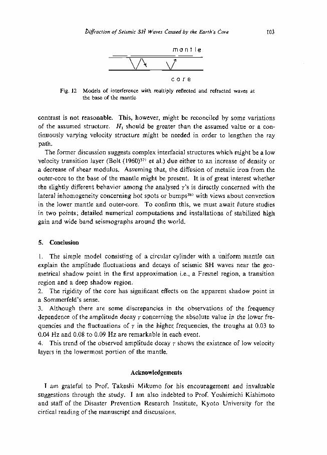
Diffraction of Seismic Sli Waves Caused by the Earth's Core 103

mantle

core

Fig. 12 Models of interference with multiply reflected and refracted waves at the base of the mantle

contrast is not reasonable. This, however, might be reconciled by some variations of the assumed structure. HI should be greater than the assumed value or a con-tinuously varying velocity structure might be needed in order to lengthen the ray

path. The former discussion suggests complex interfacial structures which might be a low

velocity transition layer (Bolt (l960)37) et al.) due either to an increase of density or a decrease of shear modulus. Assuming that, the diffusion of metalic iron from the outer-core to the base of the mantle might be present. It is of great interest whether the slightly different behavior among the analysed r's is directly concerned with the lateral inhomogeneity concerning hot spots or bumps38) with views about convection in the lower mantle and outer-core. To confirm this, we must await future studies in two points; detailed numerical computations and installations of stabilized high

gain and wide band seismographs around the world.

5. Conclusion

1. The simple model consisting of a circular cylinder with a uniform mantle can

explain the amplitude fluctuations and decays of seismic SH waves near the geo-metrical shadow point in the first approximation i.e., a Fresnel region, a transition region and a deep shadow region. 2. The rigidity of the core has significant effects on the apparent shadow point in a Sommerfeld's sense. 3. Although there are some discrepancies in the observations of the frequency dependence of the amplitude decay r concerning the absolute value in the lower fre-

quencies and the fluctuations of r in the higher frequencies, the troughs at 0.03 to 0.04 Hz and 0.08 to 0.09 Hz are remarkable in each event. 4. This trend of the observed amplitude decay r shows the existence of low velocity layers in the lowermost portion of the mantle.

Acknowledgements

I am grateful to Prof. Takeshi Mikumo for his encouragement and invaluable suggestions through the study. I am also indebted to Prof. Yoshimichi Kishimoto and staff of the Disaster Prevention Research Institute, Kyoto University for the cirtical reading of the manuscript and discussions.

104 A. SAKAI

Computations were made on a FACOM 230-60 at the Data Processing Center,

Kyoto University.

References

1) Wiechert, E.: Ober Erdbebenwellen. I. Theoretisches fiber die Ausbreitung der Erdbeben- wellen, Nachr. Ges. Wiss. Gottingen Math. Physik, B. K1, 1907, pp. 415-529.

2) Gutenberg, B.: Ober Erdbebenwellen VIIA. Beobachtungen an Registrienrugen vom Fernbeben in G6ttingen and Folgerungen Ober die Konstitution des ErdkOrpers., Nachr.

Ges. Wiss. Gottingen Math. Physik. B. KI. 1914, pp. 166-218. 3) Jeffreyes, H.: The Times of P, S and SKS and the Velocities of P and S, Monthly Notices

Roy. Ast. Soc. Geophys. Suppl. Vol. 4, 1939, pp. 498-533. 4) Dahm, C.H.: Velocity of P Waves in the Earth Calculated from the Macelwane P Curve,

1933, Bull. Seism. Soc. Amer., Vol. 26, 1936, pp. 1-11. 5) Lehmann, I.: On the Shadow of the Earth's Core, Bull. Seism. Soc. Amer., Vol. 43, 1953,

pp. 291-306. 6) Rykunov, S.L.: A Study of the Character of Diminution of Amplitudes of Waves in the

Shadow Zone of the Earth Model, Bull. Acad. Sci. USSR, Geophys. Ser., Vol. 10, 1957,

pp. 73-77. 7) Sacks, S.: Diffracted Wave Studies of the Earth's Core, 2, Lower Mantle Velocity, Core

Size, Lower Mantle Structure, J. Geophys. Res., Vol. 72, No. 10, 1967, pp. 2589-2594. 8) Alexander, S.S and R.A. Phinney: A Study of the Core-Mantle Boundary Using P Waves

Diffracted by the Earth's Core, J. Geophys. Res., Vol. 71, 1966, pp. 5943-5958. 9) Teng, T.L. and F.T. Wu: A Two-Dimensional Ultrasonic Model Study of Compressional

and Shear-Wave Diffraction Patterns Produced by a Circular Cavity, Bull. Seism. Soc. Amer., Vol. 58, No. I, 1968, pp. 171-178.

10) Teng, T.L.: Attenuation of Body Waves and the Q Structure of the Mantle, J. Geophys. Res., Vol. 73, 1968, pp. 2195-2208.

11) Shimamura, H.: Model Study on Core-Mantle Boundary Structure, J. Phys. Earth., Vol. 17, 1969, pp. 133-168.

12) Rayleigh, F.R.S.: On the Electomagmetic Theory of Light, Phil. Mag., Vol. XII, 1881,

pp. 81-101. On the Transmission of Light through an Atmosphere Containing Small Particles in Sus-

pension, and on the Origin of the Blue of the Sky, Phil. Mag., Vol. XLVII, 1899, pp. 375- 384.

13) Watson, G.N.: The Diffraction of Electric Waves by the Earth, Proc. Roy. Soc. London, A, Vol. 95, 1918, pp. 83-99.

14) Pol, B.v.d. and H. Bremmer.: The Diffraction of Electromagnetic Waves from an Electrical Point Source round a Finitely Conducting Sphere, with Applications to Radiotelegraphy

and the Theory of the Rainbow, Part 1, Phil. Mag., Vol. 24, No. 164, 1937, pp. 141-176. Part II, Phil. Mag., Vol. 24, No. 164, 1937, pp. 825-864.

15) Rubinow, S.I. and J.B. Keller: Shift of the Shadow Boundary and Scattering Cross Section of an Opaque Object, J. Appl. Phys., Vol. 32, No. 5, 1961, pp. 814-820.

16) Nussenzweig, H.M.: High Frequency Scattering by an Impenetrable Sphere, Ann. Phys., Vol. 34, 1965, pp. 23-95.

High Frequency Scattering by a Transparent Sphere., J. Mathem. Phys., Vol. 10, No. 1, 1969, pp. 82-176.

17) Duwalo, G., and J.A. Jacobs: Effects of a Liquid Core on the Propagation of Seismic Waves, Can. J. Phys., Vol. 37, 1959, pp. 109-127.

18) Phinney, R.A. and S.S. Alexander: P Wave Diffraction Theory and the Structure of the Core-Mantle Boundary, J. Geophys. Res. Vol. 71, 1966, pp. 5959-5975.

19) Phinney, R.A. and L.M. Cathles: Diffraction of P by the Core: A Study of Long-Period Amplitudes near the Edge of the Shadow, .1. Geophys. Res., Vol. 74, 1969, pp. I556-1574.

Diffraction of Seismic SE Waves Caused by the Earth's Core 105

20) Sato, R.: Amplitudes of PcP and PcS Obtained from Ray and Waves Theory Solutions and Amplitudes near Shadow Boundary, J. Phys. Earth, Vol. 17, 1969, pp. 1-12.

21) Sato, R.: Body Wave Amplitudes near Shadow Boundary-SH Waves-, J. Phys. Earth, Vol. 16, 1968, pp. 55-59.

22) Chapman, C.H. and R.A. Phinney: Diffraction of P Waves by the Core and an Inhomoge- neous Mantle, Geophys. I.R. Astr. Soc., Vol. 21, 1970, pp. 185-205.

23) Mikumo, T. and T. Kurita.: Q Distribution for Long-Period P Waves in the Mantle, J. Phys. Earth, Vol. 16, 1968, pp. 11-29.

24) Debye, P.: Näberungs Formeln ffir die Zylinderfunktionen fiir groBe Werte des Arguments und unbesehrdnkt Veranderliche Werte des Index., Miinchen, Math. Phys., B. XXXVIII, 1908, pp. 535-558.

Semikonvergente Entwickelungen ffir die Zylinderfunktionen und ihre Ausdehung ins Komplexe, Mfinchener Sitzungsberichte, B. XL, 1910, pp. 1-29.

25) Rubinow, S.I. and T.T. Wu: First Correction to the Geometric-Optics Scattering Cross Section from Cylinders and Spheres, J. Appl. Phys. Vol. 27, No. 9, 1956, pp. 1032-1039.

26) Wu, T.T.: High-Frequency Scattering, Phys. Review 2nd Ser. Vol. 104, No. 5, 1956, pp. 1201-1212.

27) Abramowitz, M., and I.A. Stegun: Handbook of Mathematical Functions with Formula, Graphs and Mathematical Tables, Dover Publication, 1965.

28) Sakai, A.: An Investigation of a Fine Structure of the Earth's Core-Mantle Interface Using Diffracted SH Waves (in Japanese) M. Sc. Thesis, Kyoto University, 1973.

29) Blackman R.B., and LW. Tukey: The Measurement of Power Spectra, Dover Publication, 1958.

30) Goldman, S.: Information Theory, Dover Publication, 1953. 31) Katsumata, M. and L.R. Sykes: Seismicity and Tectonics of the Western Pacific: Izu-

Mariana-Caroline and Ryukyu-Taiwan Regions, J. Geophys. Res., Vol. 74, 1969, pp. 5923-5948.

32) Fitch, T.J. and P. Molnar: Focal Mechanisms along Inclined Earthquake Zones in the Indonesian-Philippine Region, J. Geophys. Res., Vol. 75, 1970, pp. 1431-1444.

33) Isacks, B. and P. Molnar: Distribution of Stresses in the Descending Lithosphere from a Global Survey of Focal-Mechanism Solutions of Mantle Earthquakes, Reviews of Geo- phys. and Space Phys., Vol. 9, No. 1, 1971, pp. 103-174.

34) Isacks. B, L.R. Sykes and J. Oliver: Focal Mechanisms of Deep and Shallow Earthquakes in the Tonga-Kermadic Region and the Tectonics of Island Arcs, Bull. Geol. Soc. Amer.,

Vol. 80, 1969, pp. 1443-1470. 35) Mikumo, T.: Source Process of Deep and Intermediate Earthquakes as Inferred from

Long-Period P and S Waveforms 2. Deep-Focus and Intermediate- Depth Earthquakes Around Japan, J. Phys. Earth, Vol. 19, No. 4, 1971, pp. 303-320.

36) Sato, Y.: Study on Surface Waves VI. Generation of Love and Other Type of SH Waves Bull. Earthquake Research Inst. Vol. 30, 1952, pp. 101-120.

37) Bolt, B.A.: PdP and PKiKP Waves and Diffracted PcP Waves, Geophys. J.R. Astr. Soc., Vol. 20, 1970, pp. 367-382.

38) Morgan, W.I.: Convection Plumes in the Lower Mantle, Nature, Vol. 230, 1971, pp. 42-43.