Title Nonequilibrium Statistical Physics Young Physicists' SummerSchool 2000

Author(s) KITAHARA, Kazuo

Citation 物性研究 (2001), 75(4): 565-611

Issue Date 2001-01-20

URL http://hdl.handle.net/2433/96933

Right

Type Departmental Bulletin Paper

Textversion publisher

Kyoto University

Nonequilibrium Statistical PhysicsYoung Physicists' Summer School 2000

Kazuo KITAHARA

International Christian University

e-mail kazuo@icu.ac.jp

Summer, 2000

VfE1*~: j3~t ~ *ti'r1m~" ~1~2Jm~" ig.Jj{0)1Jt1&m~ ~ ~~5f1lr~JJ~O)t~*JiJ;. -r:~Jlt! L-r: J;.~ 0 ~ ~ ~" .:L~ r 0 ~ -0)5:k:ll.~~0)!=j:t~:" ~WO)VfEtL~~T~~~2JAT ~ 0 ~1E

1*h~£~" 1Jt1&h~~~" .I.~, )v~' -WJt~:j;JT ~96~h~~~~ c~~;J:" 1lJ~~$5tc ~1lJ~

~tl~5tc ~:5t~~tL" -ftL-f'tL~~il'7;1. - -7 ~:j;JL -r:" l~);Jfti*~" j;Jft1*fx~: J: -?-r:*fiL;f'tL ~ 0 ~ 0) m~~fiB';J:" ~ t? ~: NUrJT5f1lT5t:;fp~£* c T ~ Zubarev 0)h~~: J: ~ " ~fJ!

89~ ~p* ~ ~ t? 1P C~ ~ 0 *')v 'J 7 ~ h~£A;" ~St%ht~Jlt!~fiB~: ~ v)-r: O)1fjH5t ~ iT ~ 0

1 What is nonequilibrium1.1 Nonequilibrium Thermodynamics

1.2 External Contact . . . . . . . . .

566... 567

· 570

2 Thermodynamics of one-component fluids in motion2.1 Total energy .

2.2 Extended Gibbs relation .

570

· 570· 571

572. . . . . . . . . . . . . . . . . . 572

. .. 572

......................... 575

3 Hydrodynamics of one-component fluids3.1 Mass Conservation . . . . . . . . . . . . .

3.2 Momentum Conservation ...

3.3 Evolution equation of entropy

4 Linear response4.1 Mathematical structure of hydrodynamics

4.2 Microscopic reversibility in equilibrium ..4.3 Onsager's hypothesis .

4.4 Canonical equations for an ideal fluid . . .

577

· 579

· 583. . 583

. . 585

- 565-

5 Multicomponent fluid

5.1 Thermodynamic relation .5.2 Relaxation of diffusion flow .5.3 Hydrodynamic equations for mixture

6 Zubarev's method6.1 Deviation from local equilibrium.6.2 Kawasaki-Gunton projection formalism6.3 Mori Theory . . . . ..6.4 Nose-Hoover dynamics .

7 'Master equation and stochastic processes7.1 Stochastic processes.7.2 Markoffian process7.3 Brownian motion ..

8 Nonequilibrium fluctuations of macroscopic variables8.1 WKB method for macroscopic variables.8.2 Ehrenfest's model of random walk.8.3 Models of chemical reactions.8.4 Multivariate master equation.

9 Boltzmann equation9.1 Distribution function .9.2 H function .9.3 Local equilibrium distribution function9.4 Collision invariants . . . .9.5 Hydrodynamic equations

10 Electric conduction10.1 Correlation function method10.2 Electric conduction .....

1 What is nonequilibrium

586

· 586· 588· 588

590

· 590· 591

· 595· 595

596

. . 596

· 596· 598

599599

· 600· 601.602

602· 602

· 603.605

· 606· 606

608608

· 610

An isolated system tends to an equilibrium state, which is macroscopically static anduniform. Chemical reactions tend to an equilibrium state, where forward and backwardreactions are in balance.

A-tB

- 566-

7 c.-rD

Suppose a gas is confined in a half region of a box separated by a wall from the otherhalf region which is vacuum. When we remove the wall which separates gas and vacuum,the gas diffuses into the vauum region. This transient process is nonequilibrium with thegas flow. If one waits long enough, the whole system will be in an equilibrium state.

In order to keep a nonequilibrium state, we put the system in contact with baths, whichhave different temperatures or different chemical potentials on both sides of the system.Then heat flow or matter flow is sustained. We may also sustain velocity gradient by theshear of the two boundaries of the fluid.

In this case, viscosity is regarded as the transfer of momentum from a fast-flow regionto a slow-flow region.

When we say "nonequilibrium", it implies not only a transient state towards an equilib­rium state but also a stationary state, sustained by nonequilibrium boundary conditions.In this lecture, we first generalize entropy in order to include velocity of fluid as an inde­pendent variable of entropy. If we formulate nonequilibrium thermodynamics in terms ofentropy, we can discuss fluctuations in an equilibrium state, since by Boltzmann-Einsteinprinciple, we have the probability of having fluctuation X in the form of

This can be extended to nonequilibrium fluctuations by constructing a master equationfor the nonequilibrium probability P(X, t) "by assuming that the master equation shouldhave the equilibrium state Peq(X) = eS(X)/k.

Also, we can give a basis to "fluctuation dissipation theorem" 1 purely phenomenolog­ically. The reason why I insist on phenomenology is that it is the most sound basis ofstatistical physics and I hope to be able to extend thermodynamics to complex systems.

1.1 Nonequilibrium Thermodynamics

Here we extend thermodynamics of equilibrium systems to nonequilibrium systems. Weconsider particularly multi-component fluids. Nonequilibrum thermodynamics of solidstates has not yet been well studied. For the moment, I have no idea how to formulatenonequilibrium thermodynamics of solids which may contain defects, such as point defects,dislocations, surfaces etc.

An equilibrium system is described in terms of a set of extensive variables; internalenergy U, volume V, mass M k of the k-th component. The Gibbs relation reads

n

TdS = dU + PdV - L J-lkdMkk=l

1 This is in principle due to M. S. Green J. Chern. Phys. 35 (1956) 836.

- 567-

The Gibbs Duhem relation, which is derived from the extensivity of entropy, is

n

U + PV - L tlkMk = TSk:::;;l

n

VdP - L MkdJ-tk = SdTk:::;;l

We consider a non-equilibium system, in which there are flows of heat, matter or mo­mentum. These are caused by the spatial gradient of temperature, chemical potential orvelocity field. In order to deal with such continuum fluid, it is more convenient to usequantities per unit mass rather than absolute quantities, such as U, V and M k •

S8= M'

U1l = M'

V 1v = - =-,

M p

A f3

135]

Then we need not refer to the size of the local subsystems. By using these quantities perunit mass, we consider the system as a continuum, in which these quantities are spatiallydistributed. Then the Gibbs-Duhem relation reads,

n

U + Pv - L J-tkCk = T Sk:::;;l

n

vdP - L CkdJ-tk = sdTk:::;;l

Of course, for a one-component system, we have

{

u + Pv - J-t =Ts

vdP - dtl = sdT

Now we want to consider hydrodynamic phenomena in the framework of thermodynamics.First, we note that the viscosity is an irreversible process, in which the kinetic energy ofmacroscopic flow is transformed into internal energy. So the viscosity should be relatedto entropy production, Therefore entropyshould contain velocity as an independentvariable. Another point is that in the pres­ence of convective flow, internal energy is nomore conserved but the sum of internal en­ergy and kinetic energy is conserved. The ir­reversible transport of a conserved quantityis related to the spatial gradient of the asso­ciated intensive parameter. For example, weconsider a conserved quantity X.

- 568-

Before the transport, we have X A in the box A and X B in the box B. Thus the totalentropy before the transport is SA(XA)+SB(XB). After the transport of the amount 6.Xfrom A to B, we have the entropy SA(.XA- 6.X) +SB(XB+ .6.X). Thus the net increaseof the total entropy is

The second law requires that the transport bJ.X > 0 takes place in the spatial directionof the increasing intensive parameter. Thus in order to deal with irreversible transport ofenergy, we express the entropy as a function of total energy and the irreversible energyflow is caused by the gradient of the associated intensive parameter which will be theinverse of temperature. It should be noted that irreversible processes of non-conservedquantities obey different laws. For example, local magnetization or polarization can growor decrease without any transport. A non-conservative variable evolves in the directionof increasing entropy. So its associated intensive parameter. itself is the thermodynamicforce.

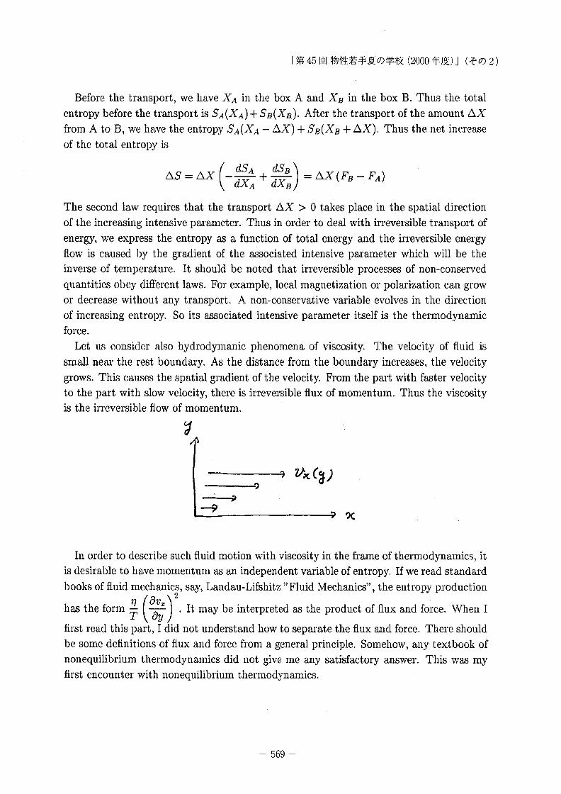
Let us consider also hydrodymanic phenomena of viscosity. The velocity of fluid issmall near the rest boundary. As the distance from the boundary increases, the velocitygrows. This causes the spatial gradient of the velocity. From the part with faster velocityto the part with slow velocity, there is irreversible flux of momentum. Thus the viscosityis the irreversible flow of momentum.

------.:j3 V'~ (d-)-----it)

?C

In order to describe such fluid motion with viscosity in the frame of thermodynamics, itis desirable to have momentum as an independent variable of entropy. If we read standardbooks of fluid mechanics, say, Landau-Lifshitz "Fluid Mechanics", the entropy production

has the form ; (0;;;)2. It may be interpreted as the product of flux and force. When I

first read this part, I did not understand how to separate the flux and force. There shouldbe some definitions of flux and force from a general principle. Somehow, any textbook ofnonequilibrium thermodynamics did not give me any satisfactory answer. This was myfirst encounter with nonequilibrium thermodynamics.

- 569-

1.2 External Contact

Depending on how a system contacts with environments, we can distinguish "isolated

system", "system in contact with a thermal bath" and "system in contact with two

different baths". In the last case, we can keep the energy flow if the two baths have

different temperature. If they have different chemical potentials, mass flow is sustained in

the system. If there is flow of energy, mass or momentum due to the contact with baths,

we may call the system" nonequilibrium open system,,2 .

Ib~ ~D

e = u+ Iv l2

2If we put 'this to the Gibbs-Duhem relation, we have

2 Thermodynamics of one-component fluids

in motion

2.1 Total energy

We consider here one-component fluids. As we noted above, internal energy u is not

a conserved variable. We constitute thermodynamics in terms of total energy instead of

internal energy.

(IVI2)p e - 2 +P - PI-l = psT

2 G. Nicolis, "Introduction to Nonlinear Science" ( Cambridge University Press, 1997)

- 570-

Then we differentiate both sides,

psdT + Td(ps) = d(pe) - d (pl"r) - pdl' -pdp + dP

Then subtracting both sides by the Gibbs-Duhem relation psdT = dP - pdj.L, we obtain

1 v 1 ( IV I2 )d(ps) = -d(pe) - - . d(pv) - - j.L - - dpT T T 2

Indeed, we have

Ivl2

Td(ps) = d(pe) - dp-2- - pv . dv - pdj.L - j.Ldp

+dP - psdT

=d(pe) - dpl~12 - v· (d(pv) - vdp) - j.Ldp

(IVI2)= d(pe) - v . d(pv) - j.L - 2: dp

Certainly this is reduced to the equilibrium relation

1 j.Ld(ps) = Td(PU) - Tdp

when there is no convective flow ( v = 0 ). In this extended Gibbs relation, we have themomentum density pv as an independent variable of entropy density ps.

2.2 Extended Gibbs relation

When we write

d(ps) = ~ Fjdajj

where CLj is the density of an extensive variable, we may call Fj intensive parameterassociated with the extensive variable aj' Thus we have the following table.

extensive variable density intensive parameter thermodynamic forces

total energy pe liT V(lIT)

momentum pv -viT -\1(vIT)

mass p - (!t - ¥) IT -\1 (j.L - ~) IT

- 571-

Since the momentum is conserved, the force which causes the irreversible flow of mo­

mentum, namely viscosity stress, is the spatial gradient of the intensive parameter -vIT.The total energy is also conserved. Thus the thermodynamic force, which causes the ir­

reversible flow of energy, namely, heat, is the spatial gredient of liT. From the extendedGibbs relation, we may discuss the viscosity phenomena in the framework of irreversibleprocess in nonequiibrium thermodynamics.

3 Hydrodynamics of one-component fluids

3.1 Mass Conservation

Fluid is an idealized concept of gas and liquid. Fluid can change its shape freely as

the boundary imposes. Real liquid behaves as fluid or as elastic body, depending on thespeed of phenomena. For a very high speed, or a very high frequency, liquid can behaveas elastic3 . For a slow motion, liquid can change its shape freely.

Fluid is charecterized by the mass density p(r,t) and the velocity v(r,t), which arefunctions of space and time. pv is the flux of mass, which passes through a unit area perunit time. Thus the mass conservation can be written as

aaP +div(pv) = 0t

This can be understood by the analogy with the continuity equation in the electromagnetictheory. The increase of the mass inside the volume V is given in terms of surface integralof mass flux pv

%t fv pdV = - fs(pv) . ndS

The right hand side can be transformed into the volume integral

- r(pv) . ndS = - r div(pv)dVis iv

3.2 Momentum Conservation

Now I explain the equation of motion of fluid. In order to obtain the equation ofmotion, we consider a mass element in the fluid which moves with a given velocity v(r, t)

3 D. Forster, Hydrodynamic Fluctuation.9, Broken Symmetry, and Correlation Function.9 (Benjamin,Frontiers in Physics 47, 1983).

- 572-

at each point of space and time. The position of the mass element at time t is denoted

as R(t) = (X(t), Y(t), Z(t)). The velocity of the mass element is the velocity of the fluid

at the position. Namely

d~?) = v(R(t), t)

If we write the component of the vector explicitly we have

/R(t)

The acceleration of the mass element is obtained by differentiating the velocity withrespect to time. For example, the x component of the acceleration is

d2X(t) ddt2 = dt vx(X(t), Y(t), Z(t), t)

= 8vx d.X(t) + 8vx dY(t) + 8vx dZ(t) + 8vx8x dt 8y dt 8z dt 8t

8vx 8vx 8vx 8vx=~vx + ~Vy + ~vz +~u:r uy uZ ut

( )8vx

= v· V Vx + 8t

For the mass element contained in a small volume dxdydz, the force acting from the other

part of the fiuid is called "stress". More precisely, we define the stress Pij as follows.

Suppose a surface Si which is perpendicular to the i-direction (i = x, y, z) at :riQ. The

force which is exerted from the part Xi > XiQ on the part Xi < XiO is denoted by a vector

Here Si is the area of the surface. Namely Sx = dydz, Sy = dzdx and Sz = dxdy.The the equation of motion, say, for the x-component is

pdxdydz~: = pdxdydz ((v. V)vx+ a~x )

= Sx [Pxx(x + d:r, y, z) - Pxx(x, y, z)]

+Sy [Pyx(x, y + dy, z) - Pyx(x, y, z)]

- 573-

and

+sz [PZX(X, y, z + dz) - Pzx(x, y, z)]

=d 'd d (8P:r.x + 8Py:c, + 8Pzx )xyz 8 8 8 .:r y z

Thus by dividing both sides by dxdydz we obtain

(( . V) 8Vx) _ (8Pxx 8Pyx 8Pzx )P v Vx + 8t - 8x + 8y + 8z .

Similar equations hold for vy and Vz .

(( . V) 8Vy) = (8Pcy 8Pyy 8Pzy)p v vy+ 8t 8x + By + 8z

(( . V) 8Vz) = (8Pxz 8Pyz 8Pzz )p v V z + at 8x + 8y + 8z

These will be combined to be written into a vector form,

If we combine with the continuity equation, we have

8(pv) 8p 8v8t = 8t v +P7fi

=-V(pv)v - p(v. V)v + V: P

=- V (pvv) + V : P

In general the stress tensor can be written as

p. - -p~ .. + II··~J - U~J ~J

The first term on the right hand side stands for hydrostatic pressure, which is negativeand always perpendicular to the surface, The second term is the viscosity tensor.

II (8Vi 8vj 2 ~ d' ) (J: d· ,.. = '11 - +. - - -u" IVV + u .. IVV

~J •/ 8 8 3 ~J ~JXj Xi

Especially when the fluid is incompressible, we have divv = O. Thus we have

- 574-

and

[a aVi a

2]

=7] --+-2VjaXi aXi aXi

In this incompressible case, we have

(( ) a'Ux) ap 2p V . V 'Ux + at = - ax + 7]"V 'Ux·

We can see that the viscosity is the diffusion of momentum.

3.3 Evolution equation of entropy

In the extended Gibbs relation for a one-component fluid

1 v 1 ( IV\2)d(ps) = -d(pe) - - . d(pv) - - fJ - - dpT T T 2 '

the derivatives denoted by d can be understood as time derivative.

a(ps) = !.. a(pe) _ v . a(pv) _ !.. (fJ _ IV I2) apat Tat Tat T 2 at

The time derivative is of the order of T = 1/ Vth, where 1 is the mean free path and Vth isthe thermal velocity Vth = JkT/m. We substitute the Navier-Stokes equation and thecontinuity equation in the second and the third terms on the right hand side. For thetime derivative of the total energy density, we substitute pe = pu + ~lvI2. Then,

a(pe) = a(pu) ~ (~lvI2) .at at + at 2

We note

= _ap ~lvl2 +v. a(pv)at 2 at

Then we can substitute the evolution equation for the density p and the momentumdensity pv. Here for the time derivative of the internal energy density, we use

a(pu) . ( ) '" aVi .-.- + dlV puv +Q = L.J Ilij - - PdlVVat .. ax)·l,)

- 575-

The term puv is the internal energy conveyed by the convective motion of the fluid. Qis heat flow. The first term on the right hand side is the viscosity heating. The kineticenergy of the convective motion is transformed into the internal energy by the viscosity.This viscosity heating term is always positive since

OViLIIij -o

.. 'i,j x)

'" (OVi OVj 2 -' . ) OVi ",'. OVi= TJ L..J -. + -" - -uijdlVV -. + ( L..J OijdlVV-,

.. ox) ox~ 3 ox)" . ox)·~J ~J

( )2 ()2TJ OVi OVj ,OVi 2. 2= - L - +- + 2TJ L - + (( - -TJ) (dlVV)2 ii=j OXj OXi i OXi 3

( )

2TJ OVi OVj 2. 2= - L -. + - + ((- -TJ) (dlVV)2 i,j OXj OXi' 3

_ TJ "', (OVi OVj) 2 I"(d' )2- - L..J - + - + ':> IVV2 i:j;j OXj OXi

2TJ [('avx avv )2 (avy avz)2 (avz av:r.) 2]+- ---- + --- + --- >03 ,ax ay ay az az ax

Thus we have the energy balance equation

a~e) +div(pev + Pv +Q - II: v) = O.

Thus the entropy balance equation is written as

a~s) + divJs =a[S]

where J s is the entropy fluxQ

J s = T + pSV

and a[S] is the entropy production rate

(1) 1 aVia[S] = Q. V - + -I:IIij-,T T.. ax)·

~,)

which can be rewritten as

- 576-

we have

Note that ~ (2-) is the thermodynamic force for the irreversible energy transport,aXj T

which is heat, and~ (-Vi) is the thermodynamie force for the irreversible momentumax· TJtransport, which is viscosity stress. As shown in the next section, these two transports

are mutually interfering.

4 Linear response

We have seen that the thermodynamic force for an irreversible transport of a con­served variable ai is the gradient of the corresponding intensive parameter Fi . Supposeirreversible flows and thermodynamic forces are linearly related. Then we can write theviscosity tensor as the linear combination of gradients of -viT and liT.

-IT .. =L"kl~ (- VI) +L"k~ (2-)~J ~J, aXk T ~J, aXk T

The right hand side can be written as

Lij,kl aVI a (1) a (1)-ITij = -r aXk - Lij,kIV/ aXk T + Lij,k aXk T

Note that the viscosity stress should be Galilei invariant. Namely, for the change ofvelocity v -+ v + u where u is the constant velocity, the viscosity stress tensor - ITij

should be invariant. If not, a bucket of water would experience different stress when thebucket is carried by constant velocity. Therefore v should appear only in the form of V'v.Thus the second and the third terms on the right hand side should cancel out.

Then we have Galilei-invariant viscosity tensor

ITij

= Lij,kl aVI

T aXk

If we compare the expression for Newtonian flow

IT (aVi aVj 2s: d' .) (S: d'.. = 71 - + - - -u·· IVV + u .. IVV

~J 'I a. a 3 ~J ~JXj Xi

Lij,kl = TTl (OikOjl + OilOjk - ~OijOkl) + T(ijOkl

For the irreversible energy flow we may put

- 577-

Then we have

For the Galilei invariance, J e should not have terms proportional to v. Thus we shouldhave

lei = Aik~ (2-) _Li,kl 8Vl8Xk T T 8Xk

As we will see soon, we have the symmetry relation

As we have seen in the expression of viscosity tensor

IT _ Lij,kl 8Vli j --T -8"

Xk

Lij,kl should be independent of velocity due to Galilei invariance. On the other hand, bythe relation

Lij.k is proportional to v. We may write as

Now note that Lij,k(v) gives the linear relation between the stress tensor and the temper­ature gradient. On the other hand, Li,kl(V) gives the relation between the heat flow andthe velocity gradient. Onsager's reciprocity requires

Therefore we can put

Thus

Hence we may write

where

is the heat flow.

- 578-

4.1 Mathematical structure of hydrodynamics

Suppose we can write the differential of entropy density ps in terms of densities of

extensive variables aid(ps) = L Fidai

i

Then we may call Fi intensive parameters. I will show that all hydrodynamic equationscan be cast into the following form

aai1:,t) =Jd3r'Mij (r,r')Fj(r') =Jd3r'Lij (r,r')Fj(r')

with the antisymmetric relation

This antisymmetry can be derived from a microscopic theory. We consider the systemconsists of N particles, whose coordinates and momenta are denoted as qI"", qN andPI' ... ,PN' The equations of motion are

dqi artdt

-api

dpi artdt

-aqi

,

which can be written in the form of Poisson's brackets

where £ is a linear operator defined by the Poisson's bracket

£f = {f, rt}

If we introduce an abbreviated notation

we may write the equation of motion as

df(t) = (£f)(t)dt

- 579-

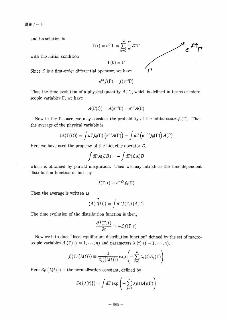
and its solution is

with the initial conditionf(O) = f

Since £ is a first-orderdifl'erential operator, we have

Thus the time evolution of a physical quantity A(f), which is defined in terms of micro­

scopic variables f, we have

Now in the f-space, we may consider the probability of the initial statesfo(f). Then

the average of the physical variable is

Here we have used the property of the Liouville operator £,

JdfA(£B) = - Jdf(£A)B

which is obtained by partial integration. Then we may introduce the time-dependent

distribution function defined by

f(f, t) == e-£t fo(f)

Then the average is written as..

(A(f(t))) =Jdf f(f, t)A(f)

The time evolution of the distribution function is then,

af(f, t) = -£f(f )at . ,t

Now we introduce "local equilibrium distribution function" defined by the set of macro­

scopic variables Ai(f) (i = 1", . ,n) and parameters Ai(t) (i = 1"" ,n).

ft(f, {'x(t)}) = ZI( {;(t)}) exp ( - ~ A;(t)Aj(r))

Here Zt({A(t)}) is the normalization constant, defined by

-580 -

The time-dependent parameters Aj (t) are defined as functions of the average values

through the condition

a;(t) = (A;), =JdfA;(r)j,(f, {A(t)}) = Z,({~(t)}) JelfA;(r) exp ( - ~ Aj(t)Aj(r))

Somehow, we will consider the situation in which the local equilibrium distribution is agood reference state as the first approximation. We define entropy of the system by

s = - kB Jdrit(r, {A( t)} ) In II (r, {A (t)} )

n

=kBIn Zl( {A(t)}) + kBL Aj(t)(Aj)tj=l

n

=kBIn Zl( {A(t)}) + kBL Aj(t)aj(t)j=l

The entropy is a function of {a( t)} through {A(t)}. Thus we have

as = kBaIn Zl( {A(t)}) + kBt aAj aj + kBAiaai aai j=l aai .

Now note that

aIn Zl ({A(t)})aai

1 aZl ({A(t)} )-

Zl( {A(t)}) oai

= 1 t OAj OZt({A(t)})Z[({A(t)}) j=l oai aAj

n aAo 1 (n)= ~ iJa; Z,( {A(t)}) Jdf(-Aj)exp - ~ AjAj

Thus we obtainas- = kBAiaai

If we compare this result with the thermodynamic relation

n

dS = LFjdajj=l

- 581 -

we may identify the parameter Aj(t) in the local equilibrium distribution function with

the intensive parameter Fj

Fj = kBAj

By the definition of ai(t) = (Ai(r)), we have

~~i =JdrAi(r) af~, t)

= - JdrAi(r)£f(r, t)

=Jdr(£Ai)(r)f(r, t).

We write f(f, t) = fl(f, t) +f'(f, t). Then we can write it as

~~i =(~~i) + (~~i). 're1J trr

where the reversible part and the irreversible part are defined by

and

( ~~i). =Jdf(£Ai)!,(f, t)lrr

Then we have

Thus it is clear that if we put

we have the antisymmetric relation

This implies

- 582-

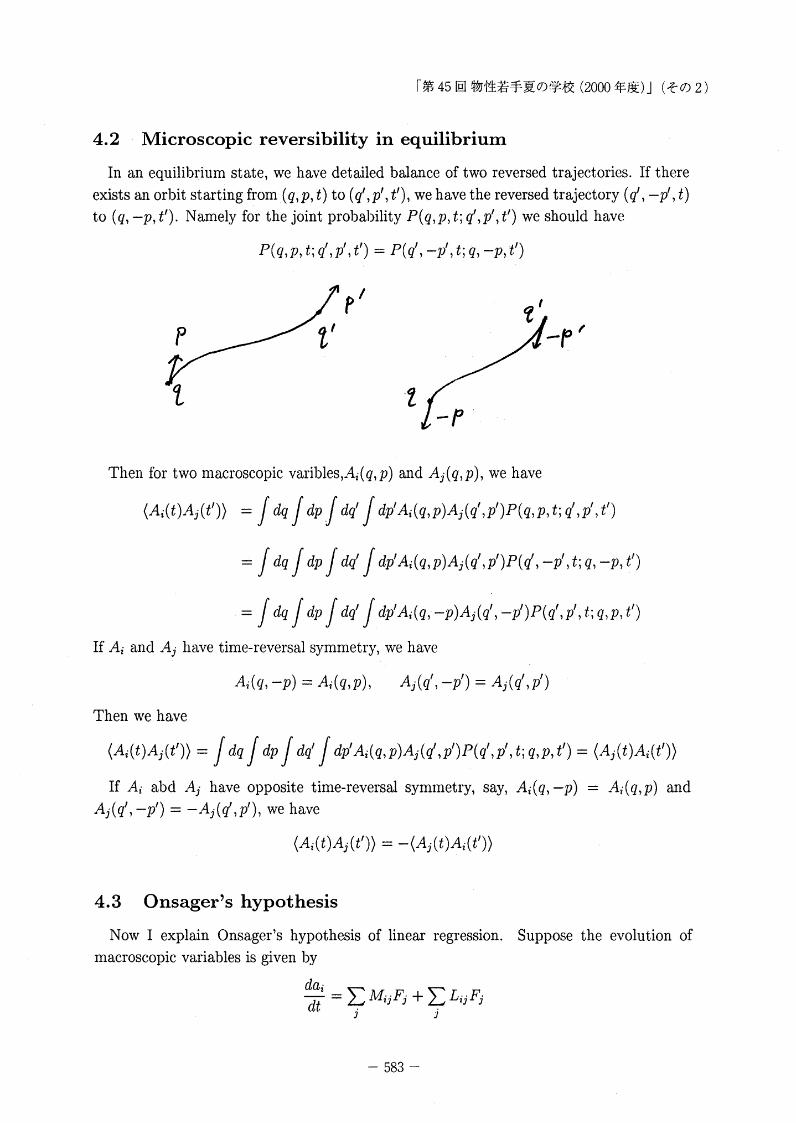
4.2 Microscopic reversibility in equilibrium

In an equilibrium state, we have detailed balance of two reversed trajectories. If thereexists an orbit starting from (q,p, t) to (q',p', t'), we have the reversed trajectory (q', -p', t)to (q, -p, t'). Namely for the joint probability P(q,p, t; q',p', t') we should have

P(q,p, t; q',p', t') = P(q', -p', t; q, -p,t')

pi

Then for two macroscopic varibles,Ai(q,p) and Aj(q,p), we have

(Ai(t)Aj(t')) =Jdq JdPJ dq' Jdp'Ai(q,p)Aj(q',p')P(q,p,t;q',p',t')

=Jdq Jdp Jdq' Jdp'Ai(q,p)Aj(q',p')P(q', -p', t; q, -p, t')

=Jdq Jdp Jdq' Jdp'Ai(q, -p)Aj(q', -p')P(q',p', t; q,p, t')

If Ai and Aj have time-reversal symmetry, we have

Then we have

(Ai(t)Aj(t')) = JdqJdpJdq' Jdp'Ai(q,p)Aj(q',p')P(q',p',t;q,p,t') = (Aj(t)Ai(t'))

If Ai abd Aj have opposite time-reversal symmetry, say, Ai(q, -p) = Ai(q,p) andAj(q', -p') = -Aj(q',p'), we have

4.3 Onsager's hypothesis

Now I explain Onsager's hypothesis of linear regression. Suppose the evolution ofmacroscopic variables is given by

dai(it = ~ MijFj +~ LijFj

J J

- 583-

This describes the approach of a macroscopic state towards the equilibrium state. Soit describes the evolution of a macroscopic nonequilibrium state. After arriving at theequilibrium state, the macroscopic state is stationary, namely time-independet. But thereexists fluctuations. If we collect the fluctuation data, which start from a given initialvalue ao, and take the average, we will get the average evolution with a given initial data.Onsager assumed that the average evolution of fluctuations obeys the same law as themacroscopic law. First note that the macroscopic evolution for a short time, we have

.) ° ['" 8S 0) '" 8S 0] 2ai(t = ai + L..t Mij~(a + L..t Lij~(a) t +O(t )j va) j va)

Onsager assumed that the average of fluctuation with a given initial condition ai(O) = a?(i = 1, ... , n) also follows the macroscopic law,

(ai(t))aO = a? + [LMij ~S. (aO) + L Lij ~S. (aO)] t +O(t2)

j va) j va)

where we put

a = (al' ... , an)

Then the correlation function in equilibrium is defined by the average over the initialconditions

This implies

(ai(t)aj(O)) = {a?a~)eq + [2: /Mij:: (aO)aZ) +2: Lij / :: (aOM ) ] t + O(t2)

) \ ) eq) \) eq

In order to calculate the average over the initial conditions, we use Boltzmann-Einsteinprinciple for equilibrium fluctuations

Peq(a) = exp [S(a)/kB]

Thus

= Jda? ... Jda~ :~aZ exp [S(a)/k B])

= kB Jda? ..Jda~a~ 8~Q exp [S(a)/kB])

J ° J °8aZ=-kB da l .. . dan 8aQexp [S( a )/kB])

- 584-

Thus we obtain

Thus we have'" (as 0 0) _~ Lij aa' (a )ak - -kBLik

3 3 eqIf ai and aj are time-reversal symmetric, we have

Thus as far as the irreversible part is concerned, we have Lij = L ji . Similarly, if ai istime-reversal symmetric and aj is anti-symmetric, we have L ij = -L ji .

For detail, see S. R. de Groot and P. Mazur4 •

Now how about the reversible part? We may make the following approximation

~ (Mi j::. (aO)a~) ~ ~ (Mij)eq (:: (aO)a2)

3 3 eq J 3 eq

~ -(1i{Ai, Ak } )eq

Thus if .41: and Ak have the same time-reversal symmetry, we have (1i{Ai1 Ad )eq = O.Ifnot,(1i{A i ,Ak })eq # 0 but antisymmetric.

4.4 Canonical equations for an ideal fluid

The reversible part of hydrodynamic equation can be formulated in an analogous wayto Hamiltonian dynamics. Let us consider irrotational flow; the velocity is given as thegradient of the velocity potential ¢.

v = '\l¢

and define the Hamiltonian by

1i =Jd3r (~lvI2 + f(p)) =Jd3r (~1'\l¢12 + f(P))

Then

81i = Jd3r (6;IV¢12 +p(V¢)V(6¢) + j'(P)6P)

= Jd3r [6P (lV:12

+ j'(P)) - 6¢V(PV¢)]

a¢ = _ 81i = _ (1'\l¢1 2f'())at 8p(r) 2 + P

ap 81iat = 8¢(r) = -'\l(p'\l¢) = -'\l(pv)

------------4 S. R. de Groot and P. Mazur, Nonequilibrium Thermodynamics(Dover, paperback).

- 585-

where we should have

The first equation is the Euler's equation for an ideal fluid. Indeed, if we take the gradientof both sides, we have

Va

¢ = -~VIV¢12 - V!'(p)at 2For example, for x-component, we have

avx a a '() 1 ap- = -\l¢. -\l¢- -f p = -v· \Iv;" ---m fu fu pfu

df = ~dPP

There are more involved formulations; see Morrison5 .

5 Multicomponent fluid

5.1 Thermodynamic relation

We consider mixture. Let M k is the mass of the k-th component. Entropy is a function

of internal energy U, volume V and masses Mk (k = 1,'" ,n).

The Gibbs relation isn

TdS = dU + pdV - L J.1kdMkk=l

The extensivity of entropy, namely the scaling

requiresn

U + PV - LJ.1kMk =TSk=l

n

SdT = VdP - L MkdJ.1kk=l

n

Let M = L lvh be the total mass. Then we introduce quantities per unit mass;k=l

S U V 1 M kS = M' U = M' v = M = p' Ck = M

-------------5 D. D. Holm, J. E. Marsden, T. Ratiu and A. Weinstein, Phys. Rep.123(1985) 1; J. E. Marsden, R.

Montgomery, P. J. Morrison and W. B. Thompson, Ann. Phys. 169 (1986) 29.

- 586-

Then we haven

U + Pv - L J.LkCk = T Sk=l

n

psdT = dP - L PkdJ.Lkk=l

Now we have ma.<:lS flow of each component, whose velocity is Vk. Thenn

V = LCkVkk=l

is the barycentric velocity. Then kinetic energy per unit mass is

n I 12 2L Ck IVkl 2 =~ + L Ck IW kl 2

k=l 2 2 k=l 2

where we introduce the diffusional velocity

W = Vk - V

Then the total energy per unit ma.'3S is

. IvI2 2 Cke=U+T+L-ilwkI2

k=l

Then we have

where we introduced a notation

Pk = PCk

for the mass density of the k-th component. From the Gibbs-Duhem relation above, wemay derive the extended Gibbs relation,

1 v n Wk n ( IvI2 IWkI2 )d(ps) = -d(pe) - - . d(pv) - L - . dJk - L J.Lk - - - - dPkT T k=l T k=l 2 2

Here we put J k = PkWk and we should note

which implies that all J k are not independent. Thus we should write

1 v n-l Wk - Wnd(ps) = -d(pe) - -. d(pv - L T . dJkT T k=l

- 587-

5.2 Relaxation of diffusion flow

Since the diffusion flows are not conserved, the irreversible process of diffusion flows of

a two-component system can be written as

dJI _ L ( WI;W2)dt - 11

for the solute species. Since the solvent fluid is abundant, we may put W2 ~ 0 due to the

condition CI WI +C2W2 = O. Thus, we have

dJ I = -£11 WI = _ £11 J Idt T TPI

where we have used PI WI = J 1. Thus we may identify the friction coefficient /'1 in

Brownian motion theory with L11 ITPl. Namely

5.3 Hydrodynamic equations for mixture

Now let us construct the hydrodynamic equations. The mass conservation is

a~k + \7 . (pVk) = chemical reaction rate

The right hand side depends on details of chemical reactions. In the following, we willdiscard chemical reactions 'unless it is necessary.

The Navier-Stokes equation for multicomponent fluid is obtained by considering themotion of a mass element of the k-th component as obtained previously for the case of

one-component fluid. Let Rk(t) is the position of a mass element of the k-th componentat time t.

Then its velocity is the velocity of the k-th component at the position

Therefore its accerelation is

Thus we may write

- 588-

The problem is to find the proper force F k per unit mass. By using the continuity

equation without chemical reactions, we have

Summing both sides with respect to k leads to an equation for the barycentric velocity

a~v) +'\1. (PVV+ ~PkWkWk+Pl-II) =0

II is the irreversible part of stress tensor. It is not at all clear whether we can assume a

simple Newtonian expression for the stress tensor as we constructed for the one-conponentfluid case.

Since we have PkVk = PkV + J k, we derive an equation for the diffusional flow J k in thefollowing form,

8Jk = (8Jk) + (8Jk)8t 8t 8t.

. nv tIT

The reversible forces described in terms of thermodynamic functions should reduce to thegredient of partial pressure - VPk in the limit of dilution of the k-th component. Indeed,

it turns out that

(8J k)8t rev

n

= -(V· v)Jk - (Jk . V)v - V(PkWkWk) + Ck L (Pk,Wk,Wk')k'=l

Enthalpy term hi. reduces to partial enthalpy hk = 88MH = 5

2kB T in the dilute limit and

k mkthe partial pressure is defined by

dTdPk = PkdJ.1k + Pk(hk - J.1k)T

Thus in the dilute limit, we have

Thus the solute is driven by its partial pressure.

The irreversible part should be

(8Jk) (1) n-l (- = LkeV - + L Lkk,8t irr T k'=l

- 589-

Suppose temperature is uniform \IT = 0 and there is no convective flow, v = O. We

assume further that the mixture consists of two components; a solute and a solvent. The

solvent is much more abundant; CI ~ C2 and W2 ~ O. We also assume that the volocity

of the solute WI is so small that we may neglect the second-order terms in WI and W2·

Then we have

where we have introdueed

kBTIII =-- In PI + ... ,

ml

When the diffusion flow becomes stationary, namely a~l ~ 0, we have Fiek's law,

J I = -D\IPI

where the diffusion constant is given by

This is called "Einstein's relation".

6 Zubarev's method

6.1 Deviation from local equilibrium

Up to now, we have discussed irreversible processes on the phenomenological ground.

There is a formulation to derive nonequilibrium thermodynamies at least fonnally6 . This

is different from Mori's theory, which derives the linear Brownian motion of fluctuationin equilibrium.

Let j(f, {A(t)}) is the distribution function in the r-space. Aj(r) is a macroscopic

variable defined in the r -space. The local equilibrium distribution jl(f, {A( t)} ) is definedby

Mr, P(t)}) - Z,t {~(t)}) exp ( - ~ Aj (t)Aj (r))

The parameters Aj(t) are determined as functions of the ensemble average aj(t) = (Aj(f))through the relations

JdrAj(f)j(f, t) =JdfAj(f)!L(f, {AU)})-------------

6 D. Zubarev, V. Morozov and G. Ropke, Statistical Mechanics of Nonequilibrium Processe.9, ·vol.l(Akademie Verlag, 1996)

- 590-

We have already seen that the reversible part of the evolution equations of thermodynamicvariables are given in terms of the local equilibrium distribution function. Now we will

estimate the other part of the distribution function f'(f, t).Zubarev introduced the following Liouville equation, which includes the coupling with

external thermal bath. The external bath drives the system into the state, which isrepresented by then local equilibrium distribution function.

ai . .- = -.ci - c(j - il)atWe assume that at the infinite past the system was exactly in a state, which is representedby the local equilibrium distribution.

lim (i - il) = 0t--oo

Namely,

lim i' = 0t-..-oo

If we substitute i = il + i' into the Liouville equation, we obtain,

af' (a)- = -(.c + c)1' - - +.c ilat at

6.2 Kawasaki-Gunton projection formalism

Now we introduce so-called "Kawasaki-Gunton" projection operator. First note that thelocal equilibrium distribution function !l(f, {A(t)}) depends on time through the param­eters {A(t)} = (AI (t)," . ,An(t)), which are again functions of {a(t)} = (al(t)," . ,an(t))due to the relation

ai(t) =JdfAi(f)!l(f, {A(t)})

Therfore from now on we write the local equilibrium distribution function as il(f, {a(t)}).Then the projeetion operator P(t) is defined by

(P(t)G)(f) = !l(f, {a(t)}) Jdf'G(f')

+~ afL(~~j~~jt)}) (J dr'G(r')Aj(f') - aj(t) Jdf'G(f'))

for an arbitrary function G(f). The projection operator P(t) is time-dependent and ithas the following properties.

- 591-

P(t)P(t') = P(t)

/ df(P(t)G)(f) = / dfG(f)

P(t)f(f, t) = f,(f, {a(t)})

p(t)af~,t) = :tf't(f, {a(t)})

The first peoperty can be proved as follows: First note

(P(t)P(t')G)(f) = f,(f, {a(t)}) / df'(P(t')G)(f')

+~ 8fI(~~}(~jt)}) (J dr'(P(t')G)(f')A; (r') - a;(t) Jdr'(P(t')G)(f'))

We also have fi·om the normalization condition

/ df(P(t)G)(f) = / dff,(f, {a(t)}) / df'G(f')

+~Jdf8M~~;{(~jt)}) (J df'G(f')A;(f') - a;(t) Jdf'G(f'))

= / df'G(f')

Furthermore

/ dfAj(f)(P(t)G)(f) =/ dfAj(f)f,(f, {a(t)}) / df'G(f')

+2: / dfAj(f) af,(f, {a(t)})k . aak(t)

x (/ df'G(f')Ak(f') - ak(t) / df'G(f'))

= aj(t) / df'G(f')

+2: aaj(t) (/df'G(f')Ak(f') - ak(t)/df'G(f'))k aak(t)

= aj(t) / df'G(f')

+ (/ df'G(f')Aj(f') - aj(t) / df'G(f'))

- 592-

This proves the first property.The second one was already proved in the proof of the first one.The third one can be proved from the definition of the projection operator,

(P(t)f)(f) = fl(f, {a(t)}) J df'f(f')

+2t aft(~~j\~it)}) (J dr'J(r')Aj(r') - aj(t) Jdr'J(r'))

8fl(f, {a(t)})=fl(f,{a(t)})+L 8.() (aj(t)-aj(t))

j aJ t

= jl(f, {a(t)})

where we have used the normalization condition

Jdff(f, t) = 1

and the definition of macrovariables

aj(t) = J dfAj(f)j(f, t)

The last property can be proved by substituting

8j = £jat

into the definition of the projection operator;

(P(t) ~{) (r) = -(P(t)£.)J(r)

= -jl(f, {a(t)}) J df'£j(f')

-2t Of, (~~j\~it)}) (J dr'£.J(r')Aj (r') - aj(t) Jdr'£.J(r'))

Now note that

and

Thus we have

Jdf£j(f, t) = 0

- J dfAj(f)£j(f, t) = d;:

(P(t) OJ) (f) = L 8!L(f, {a(t)}) daj = 8jl(f, {a(t)})

8t j aaj(t) dt at

- 593-

Then we can derive

is

Here

~' = -[Q(t)£ + e]f' - Q(t)£ft

where we have introduced another projection operator

Q(t) = 1 - P(t)

Indeed, we have

8f' = 8f _ 8fl = 8f _ p(t)8f = Q(t)af = Q(t)(-£(j +1') - e1')at at at 8t 8t 8t I

Note that P(t)f = P(t)ji from the third property. Therefore we have

P(t)1' = P(t)(f - ft) = P(t)f - P(t)fl = 0

This implies

Q(t)1' =l'This completes the proof of the evolution equation for f'.

Note also

£fl(f, t) = - L Aj(£Aj)fl(f, {a(t)})j

from the definition of the local equilibrium distribution function.We introduce an operator U(t) defined by

d ~ ~

dt U(t) = -[Q(t)£ +e]U(t)

with the initial condition U(O) = 1. Then the irreversible part of the distribution function

f'(f, t) =~ lco dt'U(t)U-1(t') Q(t')fi(f, {a(t')} )Aj(t')J

Therefore, the irreversible part of the evolution is

(d;iL= Jdf(.cAi)j'(f, t) = itL, dt' Li;(t, t'),;(t')

whereL ij =Jdf(£Ai)U(t)U-1(t')Q(t')(£Aj)fl(f, {a(t')})

Namely, the irreversible part is written as the linear combination of intensive parameters{A(t')} in the past.

Suppose we are in a stationary situation in which the intensive parameters are constant.Then we have

Lij = [Oco dt'Jdf(£Ai)U-1(t')Q(-oo)(£Aj)fl(f, {a})

is the Onsager's coefficients for non-equilibrium systems. It is not yet clear to me how itis related to the traditional Green-Kubo formula.

- 594-

I~ 45 !ill !tmtEE=FJiO)~~ (2000 1FJt)J (-f0) 2)

6.3 Mori Theory

Nlori considered the fluctuation of macroscopic variables in equilibrium. Let Ai(f) is amacroscopic variable. Suppose the system is in equilibrium. A projection operator P isdefined in terms of macroscopic variables.

PC = 2;: Ai(f) ((AA) -I) ij (AjC)J

where (AA) -1 is the inverse matrix of the matrix (AiAj ) defined by

(AiAj ) =~Jdfe-{31lAiAj , Z = Jdfe-{31l

The equation of motion of the· macroscopic variable Ai

dAi = £A·dt t

is transformed into the form of a Brownian motiondA· rt

dtt = - 2;: Jo drfij(t - r)Aj(r) + Ri(t)

J

where Ri(t) is interpreted as a random noise with the property

I:(Ri(t)Rl(O))( (AA)-l )lj = fij(t)l

which is the expression of fluctuation-dissipation theorem7 • Note the random noise doesnot follow Hamilton dynamics

Ri ( t) = eQ.et£A i

where Q = 1 - P. No one has yet succeed to create computer algorithm to simulate theprojected dynamics represented by the operator Q£. If we are interested in the dynamicsof physical quantity in the small wave number, the corresponding wave number dependentoperator Qk£ becomes £ itself. However, it is not clear whether we can take this limitfirst before the final expression for the transport coefficient is reached8 .

6.4 Nose-Hoover dynamics

In order to compute dynamics of particles in contact with a heat bath, Nose inventedthe following equations,

7 R. Kubo, M. Toda and N. Hashitsume, Statistical Physics II (Springer)8 D. J. Evans and G. P. Morris,"Statistical Mechanics of Nonequilibrium Liquids" (Academic Press,

1990).

- 595-

where ex depends on the dynamical state of all particles

ex = 2;:PiFi({q})/ 2;:p;t t

This choice assures that the kinetic energy of particles is conserved

L PT = constanti

This Nose-Hoover dynamics assures the convergence of transport coefficients in the rep­resentation of correlation functions. However, there is a serious problem; Nose-Hooverdynamics does not assure lotal conservation of momentum.

7 Master equation and stochastic processes

7.1 Stochastic processes

When we discuss fluctuations, the probabilistic description is appropriate9 . SupposeX(t) is a fluctuating variable, called "random variable". The probability of having .Tl <X(td < Xl + dXl is denoted by Pl(Xl,tl)dxl' Similarly the probability of having Xl <X(tl) < Xl + dXl and X2 < X(t2) < X2 + dX2 is denoted by P2(X2, t2; Xl, tl)dxldx2. Wecan define Pn(xn,tn;· .. ;Xl, tl) similarly. We define "conditional probability"

Namely, it is the probability of having Xn < X(tn) < Xn + dXn under the condition thatwe had .X(td = .Tl, ... ,.X(tn-d = Xn-l.

7.2 Markoflian process

The Markoffian process is defined by

In this case, we have Chapman-Kolmogorov equation

JdX2T(X3' t31 x2, t2)T(X2, t2l x l, td = T(X3' t3l x l, td

The conditional probability for a short time interval b..t is estimated to be

9 Wax, Selected Papers on Noise and Stochastic Processes (Dover, paperback)

- 596-

where

Normalization condition requires

Thus we may write

TV(XI --+ X2) is called "transition probability", but I prefer to call it "transition rate"since it is not probability in the sense of normalization. This gives the transition rateper unit time. If we substitute this expression into Chapman-Kolmogorov equation, weobtain "master equation" ,

ap~~, t) == _ Jdx'W(x --+ x')P(x, t) + Jdx'W(x' --+ x)P(x', t)

This can be rewritten in the form of "Kramers-Moyal expansion"

ap(x, t) = f (-l,)n (~) nCn(x)P(x, t)at n=l n. ax

Cn(x) =JdrW(x --+ x + r)rn = lim ~ JdrT(x + r, tlx, 0)t-O t

The last equality comes from the definition of the transition rate in terms of the shorttime expansion of the conditional probability. Therefore, we may write

Here (.. ')x(O)=x is the average with a fixed initial value (0) = x. This interpretation isused when we derive a master equation from a mechanical equation of fluctuation. Forexample, we consider the Langevin eqaution

dxdt = F(x) + R(t)

Then we have

- 597-

Therefore

(x(t) - x)

Thus we haveC1(x) =F(x)

and from the second moment, we obtain

where we put

7(lt) J tU.~--.;;./

~ ~at1tr4{.

7.3 Brownian motion

Let u be the velocity of a solute particle in a solvent.

dum dt = -,mu + R(t)

with (R(tl)R(t2)) = 2Du b(tl - t2)' The master equation becomes "Fokker-Planck" equa­tion,

ap =~ (,u+ Du~) pat au m2 auThe steady state solutionwith the boundary condition lim P(u, t) = 0 should be Maxwellian

lul-oo

(mU

2)Peq(u) ex exp - 2k

BT

Therefore we have to put

D == lim ((x(t) - X(O))2)t-oo 2t

This is called "Fluctuation-dissipation theorem". The diffusion constant is also estimatedfrom this model by noting

and

x(t) - x(O) = l t

dru( r)

The result is

which is called "Einstein's relation" .

- 598-

8 Nonequilibrium fluctuations of macroscopic

variables

8.1 WKB method for macroscopic variables

We consider a macroscopic system, described by a variable X, which is extensive in thatit is proportional to the size of the system n. When the variable changes, X -+ .x + T, T

is microscopic. X may be the population of a town. T is the number of new-born babies.The town consisits of many subregions, each of which can give birth to some babies. Thusthe size of the town increases, the probability of finite increment l' per unit time increasesin proportionality to the size of the system n and may be dependent on the density ofpopulation x/no Thus the transition rate should have the form

VV(.X -+ X +1') =Ow (~;1')

Then we have for the scaled probability distribution function P(x, t),

8P-8 = -0 L (1 - e-(r8/8x)/H) l:(X; r)P(x, t)

t 7'

which may be rewritten in a familiar form

18P (1 8)Oat=-H x'08x P(x,t)

where the "Hamiltonian" is defined by

H(x,p) =L (1 - e- rp) w(x; 1')

r

In analogy with quantum mechanics, we use "WKB approximation",

P(x, t) =A(:r, t)eH</J(X,l)

Then we have "Hamilton-Jacobi equation" .

If we make further a Gaussian approximation

)1 2¢(x t = --(x - y(t)) + .... , 20"(t)

we obtain a closed set of equations,

- 599-

Then we have

8.2 Ehrenfest's model of random walk

Let us consider a one-dimensional lattice consisting of 2N +1 sites. Suppose a particleis at site M. The transition rate for M ~ M ± 1 is given by

IW(M - M + 1) = :(N - M)

vV(M ~ M -1) = -(N +M)7

Suppose we have a large lattice, N ~ 00, and put x = MIN. Then we may write

NW(M ~ M + 1) = 27(1- x) = Nw(x,+l)

NW(M ~ M -1) = 27(1 + x) = Nw(x, -1)

ICl(X) = ~~

C2(x) = -7

The equations for y(t) and O"(t) are easily obtained,

dy-

dtYT

dO" 2dt =-:;: (0" - 1)

Namely, the model converges to a Gaussian distribution. We may apply a general methodof Hamilton - Jacobi equation; solve the caconical equations

dx 81idt = lJp

dp 81idt = - ax

- 600-

with the Hamiltonian

H(x,p) = 21r [(1 - e-p

) (1- x) + (1 - eP) (1 + x)]

The phase flows look like the figure below.

8.3 Models of chemical reactions

Suppose there is a reaction of the scheme,

A~X, X~A

Let X be the number of X molecules. Then the transition rates are

{

vV(X ~ X + 1) = kA

lV(.X" ~ X-I) = k'X

Let 0 be the size of the reactor and xXjO and a = AjO are the concentrations. Thenwe may put

{

W(X ---. X +1) = nka = nw(x; +1)

vV(X ~ X-I) = Ok'x = Ow(x; -1)

If the system is closed, one should be careful since A also changes with A + X ­N(total number of molecules). Then we have a different transition rate

{

W(X,A~X+1,A-1)=kA

W( X, A ~ X-I, A +1) = k'X

- 601 -

8.4 Multivariate master equation

If the master equation as the following transition rate

W({X} ~ {X+r})=Ow({x};{r})

with Xi = Xi, we haveClI.:({x}) = I>'kW({X}; {r})

{r}

C2kl({X}) = I>'krlw({X}; {r}){r}

The evolution equations are

dYk { }Cit = C1k( Y )

d;t = L (I<kmuml + (JkmKlm) +C2k1 ( {x})m

with

9

9.1

, aClkI\.km =~

uXm

Boltzmann equation

Distribution function

We denote by f( c, r, t )d:3cd3r the number of particles with velocity and position within

a small region d3cd3r in the ~t-space. By this definition, we have

where N is the total number of particles,

n(r,t) =Jf(c,r,t)d3c

in the number density, If there is no collision, we have

f(c, r, 0) = f(c, r + ct, t)

Thus if we take time-derivative, we obtain,

of of-+c,-=Oat or

- 602-

If we take the collision effect into account, we should get

8f (8f )-+(c'\I)f= -at at coll

The collision term

( 8f

) =Jd3c'Jd3CI Jd3c~u(ccdc'cDf(c',r,t)f(c~,r,t)at coil

= - Jd3c'Jd3CI Jd3C~u(c'C~ICCI)f( c, r, t)f(CI, r, t)

The scattering rate has the following symmetry due to the time-reversal symmetry of

collision process

U(C'C~ICCI) = u( -c - cII- c' - c~)

Furthermore due to the space-reversal symmetry we have

Therefore we have

u(c'c~ IccI) = u(ccdc'cD

We introduce the following abbreviated notations

f = f(c,r,t), it = f(CI,r,t), f' = f(c',r,t), f~ = f(CI,r,t)

Then the collision term becomes

9.2 H function

Now we introduce "H function" defined by

H (r , t) =Jd3Cf In f

Then we have

= -\I. Jd3c(cflnf) +Jd3c (it) (Inf + 1)coll

- 603-

We may call

J H =Jd3c(cflnf)

"H flow". Then we have We may call

Note

Jd3c (8f ) = 08t coli

Therefore

X (/'f: - f Ii) In (;'~J ::; 0

The last inequality comes from the fact that for Va, Vb > 0, we have

(a-b)ln(~) <0

The equality holds only if f' ff = f II·Especially when f is independent of r, namely the system is homogeneous, we can prove

the system will be in an equilibrium state. Let the equilibrium distribution function be

(m )3/2 (m 1vI2 )

feq = n 27rkBT. exp - 2k

BT

Then we can show that the H function, defined by

H(t) = Jd3cfln (f.J

has the following properties

1. H ~ 0 and the equality holds only when f = feq.

dH .2. dt ~ 0 and the equalIty holds only when f = feel'

Thus feq is the asymptotic limit of f for t --t 00.

- 604-

9.3 Local equilibrium distribution function

Let us go back to the inhomogeneous situation. The H function takes a stationary value

when we have 1"f~ = f fI· Since the consition of 0"(c'c~ Iccl) requires

2. c + Ct = c' + c;

the function f which satisfies 1"ff = ffl should be of the following form,

f(O)(c,r,t) = exp (Alcl2 + B· c+ C)

If we choose the parameters A, Band C,we may write

( )

3/2 ( I ()1 2)'(0) _ m m c - v r, t

f (c,r,t)-n(r,t) 21rkBT(r,t) exp - 2k

BT(r,t)

This is called local equilibrium distribution function.To see 1"ff = f fI implies the local equilibrium, we assume first that f(O) is of the form,

Then we have

Thus we may assumeG(C)G(Cl) = G(c')G(cD

F(lcj2)F(lclI2) = F(lc'12)F(lc; 12)

Then the task is to determine the function f(:r), which satisfies f(x)f(y) = f(z)f(x+y­z). If we differentiate both sides with respect to x, we have 1"(x)f(y) = f(z)1"(:r+y-z).Then we put x = z = O. We obtain 1"(O)f(y) = f(O)1"(y). This implies f(x) is anexponential function.

The parameters n(r, t), T(r, t) and v(r, t) are defined by the distribution functions

Jd3cf = n

- 605-

and we have the following relations

9.4 Collision invariants

A funetion <p(c) is eaJled "eollision invariant" if it satisfies

Jd3

c<p (~) =0coil

In faet, we ean prove the following relation by using the symmetry of (J,

Thus the eollision invariant implies

<p(c) + <p(Cl) = <p(c') + <p(c;)

Therefore there are five eollision invariants

1

<p(c) = c

9.5 Hydrodynamic equations

The eollision invariants are closely related to hydrodynamies1o We may write

10 P. Resibois and M. DeLeener,Clas.~ical Kinetic Theory of Fl'uids (John-Wiley, 1977).

- 606-

Then we have

Thus

aat (n(<p) ) + "V . (n (<pc)) = 0

Namely the collision term does not appear explicitly and the resulting equation takes theform of a conservation law.

For example, if we choose <pl,we have

an-+"V·(nv)=Oat

If we put p = mn we oftain the mass conservation

ap- + "V . (pv) = 0atIf we choose <p = c we obtain

If we put

and p = mn, we obtain

If we compare it with the hydrodynamic equation, we can conclude

Suppose the distribution function f, which is the solution of the Boltzmann equation, canbe written as

f = feD) + 1"we can write

The local equilibrium is a Gaussian distribution around the average velocity, we can easilycalculate the local equilibrium average

(0) pkBTp((Cj - Vj)(Ci - Vi)) =Oij-- = oijnkBT = POij

mThis is hydrostatic pressure. Therefore we can identify the viscosity tensor

- 607-

If we choose <p = lel2, we have

We put againe=v+(e-v)

we have

Thus if we identify

we have

Next we note

Then we will get

3 .pu = ~(Ic - v1 2

) = "2nkBT

(leI 2e) = Ivl 2v + (Ie - vl 2 )v

+2v· ((e - v)(e - v)) + (Ie - vl 2 (e - v))

a~e) + \7. (pev + pv. ((e - v)(e - v)) + ~(Ic - vl 2(e - v))) = 0

Therefore if we identify this with the energy balance equation, we can put

This is heat current.

10 Electric conduction

10.1 Correlation function method

The hostory of research of transport theory in Japan was thoroughly studied by Ichiyanagi11,

who passed away leaving us his last Japansese monograph12 . The electric conduction is

a thermodynamic phenomena in which matter flows inside a medium, which is subject to

the boundariesy with different chemical conditions o

However, in Kubo's formula, this thermodynamic point was not taken. At infinite past,

the system was in equilibrium with a given temperature, i. e., in canonical ensemble.

11 M. Ichiyanagi,"Conceptual developments of Non-equilibrium statistical mechanics in the early daysof Japan", Phys. Rep. 262 (1995) 227-310

12 -1»PJE*IJ, r~w¥~*:fC~t:;l]~J

- 608-

Then the system was separated from the bath and an external field was switched on and

gradually set stronger. Then a matter flow is established at time t = O. Therefore, itis natural to suppose that the temperature of the system is raised due to Joule heat­ing but this effect is considered to be of the second order with respect to the electricfield. The mechanism of establishing steady electric current in such an isolated systemis not at all dear. There are theoretical investigation concerning the existence of such anonequilibrium steady state, called BSR(Bowen-Sinai-Ruelle) condition.

We denote the charge of a particle by q and the electric field by E. The position and

the momentum of a partide are denoted by qi and Pi' The perturbation Hamiltonian is

N

H'(t) = -qE(t) . L qii=l

The generalization leads toH'(t) = -F(t)A(f)

The dynamics intrinsic to the system is described by Ho. Then the Liouville equation is

~{ = {H(t), f} = -£(t)f

where corresponding to the Hamiltonian

H(t) = Ho + H'(t)

we have

£(t) = £0 + £'(t)

We write the distribution function as

f = feq + j'(t)

The in the first-order approximation we have

al' '( ) '( )at = -£of t -£ t fell

Since the system is in equilibrium at infinite past, we have

lim j'(t) = 0t->-ooThus we have

j'(t) = - J~oo dse-£o(t-s)£'(s)feq

We observe a quantity B(f), whose equilibrium value is supposed to vanish.

(B(f))eq = 0

- 609-

Then

We note

and

We write

Then we have

Here we call

(B(f)) =JdfB(f)j'(f, t)

= - [00 ds JdfB(t - s)£'(s)feq

.c'(s)feq = -{H'(s),feq} = F(s){A,feq} = F(s) :!::o {A, Ho}

dfeq feqd1io = - kT

(B(f)) = k~ [00 ds JdfB(t - s)F(s)feqA

=[00 dsiI?(t - s)F(s)

1 .iI?(t) = kT (B(t)A)

"response function" .

10.2 Electric conduction

For the case of electric conduction, we choose

A = qLqi' B =q~ ~b(qi - r) = J(r)i t

Then we have. " . "qi J 3A=q~qi=q~m= drJ(r)=J

t t

andF(t) = E(t)

Therefore the response function is expressed as the correlation function of current.

(B(t)A) = (J(r, t)J) = ~J(t)J(O))

- 610-

If we specify the time-dependence of the electric field as

we obtain(JAr, t)) = EO(J(w)eiwt+ct

Here the conductivity

q2N roo(J(w) = kTV J

odt(Vlx(t)Vlx(O))e-(iw+c)t

For DC electric field we have

is now frequency dependent. When charged particles move independently of each other,we have

The theory of Brownian motion predicts that the diffusion coefficient is given interms of

velocity correlation function of a particle

Thus we have

(J(O) = q:n:This gives the relation between diffusion coefficient and conductivity for a dilute carriercase.

- 611-