title of the paper - agecon searchageconsearch.umn.edu/bitstream/170682/2/aaea submission.pdfinto...
TRANSCRIPT

Title of the Paper
The Public Benefits of Private Technology Adoption
Author, Author Affiliation, and Author email
Anil K. Bhargava, University of California, Davis [email protected] Travis J. Lybbert, University of California, Davis
David J. Spielman, International Food Policy Research Institute
Selected Paper prepared for presentation at the Agricultural & Applied Economics Association’s
2014 AAEA Annual Meeting, Minneapolis, MN, July 27‐29, 2014. Copyright 2014 by [authors]. All rights reserved. Readers may make verbatim copies of this document
for non‐commercial purposes by any means, provided that this copyright notice appears on all such
copies.

The Public Benefits of Private Technology Adoption
Anil K. Bhargava, Travis J. Lybbert and David Spielman
May 2014
1 Introduction
The recent acceleration of climate change due to global warming has been linked to erratic and
extreme weather patterns around the globe. India’s drought in 2012 was its fourth in the previous 12
years, and the United Nations World Meteorological Society projects the frequency, intensity and
duration of these to increase. Moreover, future monsoon rains–on which Indian agriculture relies–
are expected to be heavier but shorter in duration, reducing the amount of water table recharge.
Among the most vulnerable to the fallout from these climate changes are the poorest farmers who
have the fewest opportunities to adapt through alternative livelihoods or adopting conservation
agriculture techniques. Much has been written about possible reasons for low uptake of high
return agricultural practices, such as the higher risk, lack of information, liquidity constraints, and
credit and insurance market failures.
This paper builds on recent analyses of farmer demand and private returns to resource conserv-
ing technology in India by evaluating total benefits inclusive of those accruing to nonadopters. In
particular, it aims to measure the public benefits to small Indian farmers of private water-conserving
agricultural technology adoption in their village. We study the agricultural land preparation tech-
nology laser land leveling (LLL), which has been shown to decrease water usage by 26% on flood-
irrigated staple-crop lands. Private benefits to this technology are captured by reduced expenditures
1

on diesel needed to fuel pumping. We measure additional public benefit on pumping costs to non-
adopters stemming from the changes in water table depth caused by the adopters.
We estimate public impacts by building hydro-economic models that capture how water ta-
bles may be affected by private adoption. This can either happen broadly through aquifer-wide
withdrawal and recharge of water tables or more locally around water wells, where the size and
duration of temporary cones of depression formed during pumping can interact with neighboring
pumps and affect the withdrawal process. In this analysis, we specify a model that allows for
both of these channels in generating spillover effects from adopters to nonadopters. The model
we develop here resembles some of the modeling in Madani and Dinar (2012), which focuses on
numerical analyses of groundwater management systems to see how altering private incentives can
lead to improved public water use.
In terms of common pool resources, whether one can expect an impact from adopters to non-
adopters through either of these channels depends on the nonexcludability and subtractability of
the resource (Ostrom, 1995). In terms of LLL, both water table extraction and digging water wells
that lead to interacting cones of depression are nonexcludable: anybody can access the water un-
derground and anybody can set up a pump if they are financially able. However, while cones of
depression within a close enough radius are subtractable, it is not clear that extraction from wa-
ter tables necessarily affects their neighbor’s hydraulic head, even if hydraulic conductivity rates
are low. We do not try to completely measure impacts through water table extraction but instead
adjust the weight that each of these channels receive in our model in generating spillover effects.
Methodologically, these two channels involve several overlapping explanatory variables, such as
soil type, rainfall, geographical positioning, and technology use.
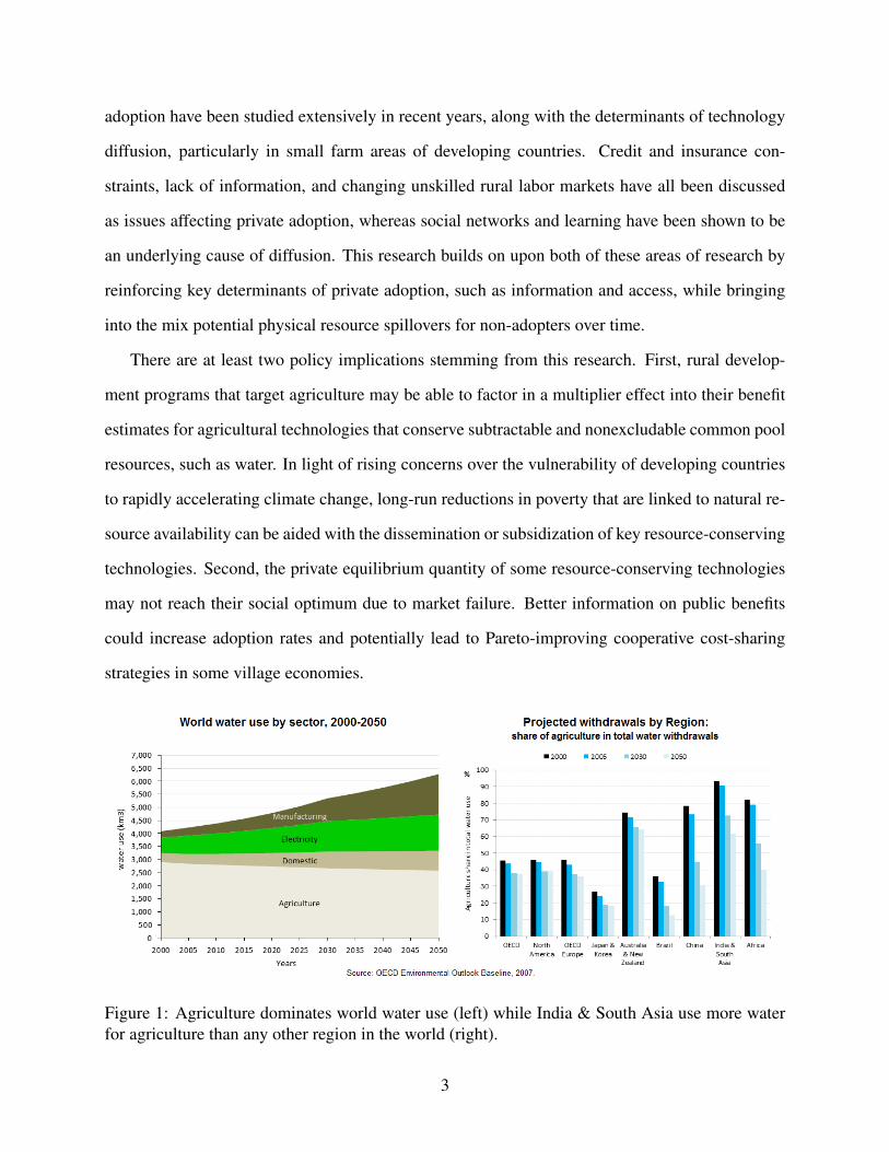
Results from this research have the potential to impact agricultural development policy in India,
where overextraction is becoming a more severe problem in a country that already has the highest
share of public water going to agriculture (see Figure 1). The diffusion of resource-conserving
technologies not only has an immediate impact on the poverty of individual farmers but also on
farmers unable to adopt both now and in the future. The determinants of agricultural technology
2
adoption have been studied extensively in recent years, along with the determinants of technology
diffusion, particularly in small farm areas of developing countries. Credit and insurance con-
straints, lack of information, and changing unskilled rural labor markets have all been discussed
as issues affecting private adoption, whereas social networks and learning have been shown to be
an underlying cause of diffusion. This research builds on upon both of these areas of research by
reinforcing key determinants of private adoption, such as information and access, while bringing
into the mix potential physical resource spillovers for non-adopters over time.
There are at least two policy implications stemming from this research. First, rural develop-
ment programs that target agriculture may be able to factor in a multiplier effect into their benefit
estimates for agricultural technologies that conserve subtractable and nonexcludable common pool
resources, such as water. In light of rising concerns over the vulnerability of developing countries
to rapidly accelerating climate change, long-run reductions in poverty that are linked to natural re-
source availability can be aided with the dissemination or subsidization of key resource-conserving
technologies. Second, the private equilibrium quantity of some resource-conserving technologies
may not reach their social optimum due to market failure. Better information on public benefits
could increase adoption rates and potentially lead to Pareto-improving cooperative cost-sharing
strategies in some village economies.
Figure 1: Agriculture dominates world water use (left) while India & South Asia use more waterfor agriculture than any other region in the world (right).
3

2 Background
All of India’s major rivers originate either from the Himalayas, Vindhya and Satpura ranges in the
middle of the country, or the Sahyadri or Western Ghats along the western coast. Most of India’s
seven main rivers and their tributaries pour into the Bay of Bengal to the east, though some go west
into the Arabian Sea and others have inland drainage from Ladakh through the Aravali mountain
range and deserts of Rajasthan.
In Uttar Pradesh, the rivers flow west to east mostly from the Himalayas. The two main rivers
are the Ganges (or Ganga) and the Ghaghra. The Ganga flows through the heart of the state–from
northwest to southeast–until it merges with the Yamuna in Allahabad, then absorbs the Gomti
River near Varanasi, and finally leaves the state for Bihar at Patna just south of Deoria district in
eastern U.P. The Ghaghra River starts in southwestern Nepal and flows into the Ganges in Bihar but
not before converging with the Rapti River, which flows along the southwestern border of Deoria
starting near Rudrapur, at Barhai and flowing along the southern border of Deoria for roughly
50 kilometers. The Gandaki River also starts in Nepal and flows on the northeastern border of
Maharajganj. The smaller Rapti River flows within the southwestern portion of Maharajganj.
Figure 2: River flow through sample area. Source: Wikimedia Commons
4
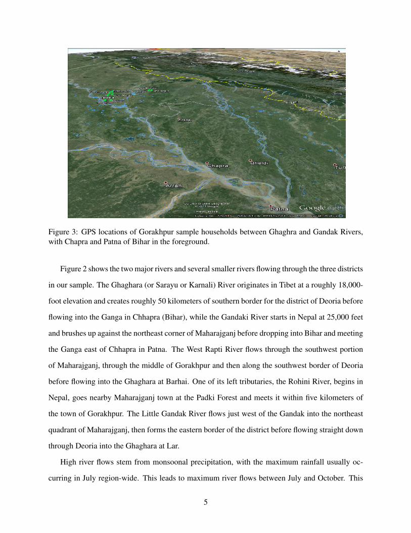
Figure 3: GPS locations of Gorakhpur sample households between Ghaghra and Gandak Rivers,with Chapra and Patna of Bihar in the foreground.
Figure 2 shows the two major rivers and several smaller rivers flowing through the three districts
in our sample. The Ghaghara (or Sarayu or Karnali) River originates in Tibet at a roughly 18,000-
foot elevation and creates roughly 50 kilometers of southern border for the district of Deoria before
flowing into the Ganga in Chhapra (Bihar), while the Gandaki River starts in Nepal at 25,000 feet
and brushes up against the northeast corner of Maharajganj before dropping into Bihar and meeting
the Ganga east of Chhapra in Patna. The West Rapti River flows through the southwest portion
of Maharajganj, through the middle of Gorakhpur and then along the southwest border of Deoria
before flowing into the Ghaghara at Barhai. One of its left tributaries, the Rohini River, begins in
Nepal, goes nearby Maharajganj town at the Padki Forest and meets it within five kilometers of
the town of Gorakhpur. The Little Gandak River flows just west of the Gandak into the northeast
quadrant of Maharajganj, then forms the eastern border of the district before flowing straight down
through Deoria into the Ghaghara at Lar.
High river flows stem from monsoonal precipitation, with the maximum rainfall usually oc-
curring in July region-wide. This leads to maximum river flows between July and October. This
5

seasonal distribution of flows is similar for all the river basins in the region. The snowmelt con-
tributes to the flow in the snow-fed rivers considerably both during dry and pre-monsoon seasons
when there is less rainfall but higher temperature conditions. Although river flow is highly cor-
related with annual precipitation, monthly flows are not as tightly correlated due to lags in runoff
time, site-specific rainfall amounts, and the indirect relationship between rainfall input and catch-
ment runoff output due to hydrological storage.
Uttar Pradesh is the most populated state in India, partially because of the fertile Indo-Gangetic
Plains (IGP) that make up much of the area. Our sample districts are in the middle of the the IGP.
Figure 5 shows our sample area, which is located in the eastern part of the state, just south of the
Nepal border and west of Bihar. Figure 5 shows how our sample villages (eight per district) are
spaced within each district and Figure 3 shows the exact GPS coordinates of many of our sample
households across all three districts.
Figure 4: Location of eastern Uttar Pradesh districts and spacing of sample villages within districts.
6
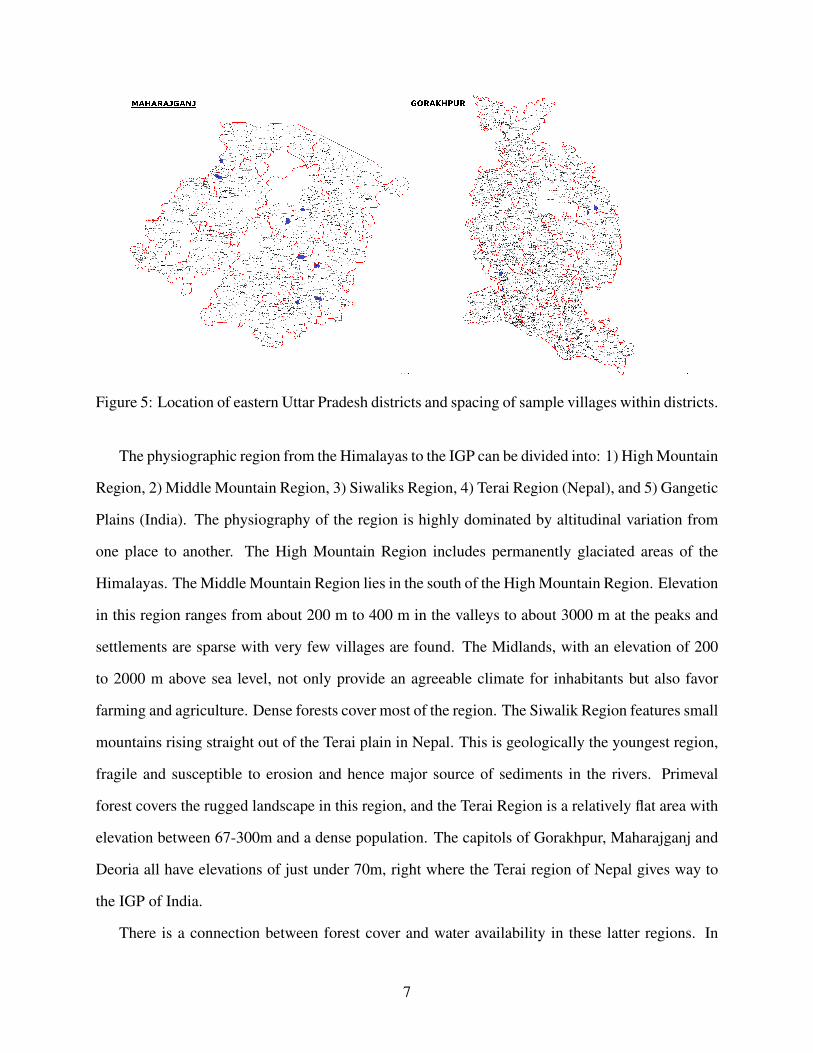
Figure 5: Location of eastern Uttar Pradesh districts and spacing of sample villages within districts.
The physiographic region from the Himalayas to the IGP can be divided into: 1) High Mountain
Region, 2) Middle Mountain Region, 3) Siwaliks Region, 4) Terai Region (Nepal), and 5) Gangetic
Plains (India). The physiography of the region is highly dominated by altitudinal variation from
one place to another. The High Mountain Region includes permanently glaciated areas of the
Himalayas. The Middle Mountain Region lies in the south of the High Mountain Region. Elevation
in this region ranges from about 200 m to 400 m in the valleys to about 3000 m at the peaks and
settlements are sparse with very few villages are found. The Midlands, with an elevation of 200
to 2000 m above sea level, not only provide an agreeable climate for inhabitants but also favor
farming and agriculture. Dense forests cover most of the region. The Siwalik Region features small
mountains rising straight out of the Terai plain in Nepal. This is geologically the youngest region,
fragile and susceptible to erosion and hence major source of sediments in the rivers. Primeval
forest covers the rugged landscape in this region, and the Terai Region is a relatively flat area with
elevation between 67-300m and a dense population. The capitols of Gorakhpur, Maharajganj and
Deoria all have elevations of just under 70m, right where the Terai region of Nepal gives way to
the IGP of India.
There is a connection between forest cover and water availability in these latter regions. In
7

the Terai and hill areas, forests decreased at an annual rate of 1.3% between 1978 and 1979, and
2.3% between 1990 and 1991. As the Terai is increasingly deforested, drained and brought under
cultivation, an evolving permeable mixture of gravel, boulders, and sand enables the water table
to sink deeper. On the other hand, where the Terai zone is composed of less permeable layers of
clay and fine sediments, groundwater rises to the surface in springs and wetlands, causing heavy
sediment load to fall out of suspension. This enables the frequent massive floods in the greater
region as monsoon-swollen rivers overflow their low banks and and rich sediment is washed away.
The 2008 Bihar flood was an example of this.
Broadly, the IGP itself can be divided into two drainage basins by the Delhi Ridge; the west-
ern part consists of the Punjab Plain and the Haryana Plain, and the eastern part consists of the
Ganga–Bramaputra drainage systems. This divide is only 300 meters above sea level, causing the
perception that the IGP appears to be continuous between the two drainage basins. The middle
Ganga plain extends from the Yamuna River in the west to the state of West Bengal in the east.
The lower Ganges plain and the Assam Valley are more verdant than the middle Ganga plain. The
lower Ganga is centered in West Bengal, from which it flows into Bangladesh. Some geographers
subdivide the Indo-Gangetic Plain into more parts based on regional availability of water. These
include the Indus Valley Plain, the Punjab Plain, the Haryana Plain, and the middle and lower
Ganges Plains.
U.P.’s climate is primarily defined as humid subtropical with dry winter, though parts of eastern
U.P. are classified as semi-arid. Though the IGP gives a predominantly single climatic pattern, U.P.
has a climate of extremes with temperatures fluctuating between 0 °C to 50 °C in several parts of
the state and cyclical droughts and floods due to unpredictable rains. The region is dependent
on the southwest monsoon, with rains varying from an annual average of 1700mm in hilly areas
to 840mm in Western U.P. Because most of this rainfall comes within those four months, excess
rain can lead to floods and shortages can lead to droughts, causing these two situations to happen
frequently in the state, especially as weather patterns become more erratic.
The population densities in the Uttar Pradesh and Bihar portions of the IGP are 415 and 760
8

persons/km2, respectively. The main occupation is agriculture, since the entire catchment is cul-
tivable with rabi crops dominating the agricultural pattern. The area is practically devoid of any
mineral resources except limestone, which are found in the form of marls in the Unnaw and Bara-
banki districts of Uttar Pradesh. There is little industry in the area, though a few small-scale
industries are based on agriculture or forest produce.
3 Model
3.1 Impact through groundwater recharge
One of the most prominent equations relating plot characteristics to water table recharge is Darcy’s
Law. The viscosity of fluid and pressure drop over a given distance determine the fluid’s discharge
rate through a porous medium. The porosity of the medium is determined by its permeability and
the area over which the fluid flows. In the most general form,
Q =−kA(Pb−Pa)
µL, (1)
where Q is the total fluid discharge (m3/s), k is the intrinsic permeability of the medium (m2), A is
the cross-sectional area to flow (m2), (Pb−Pa) is change in pressure drop of the area in question
(in pascals), µ is the fluid viscosity (in pascal-seconds), and L measures the length over which the
pressure drop is taking place (m).
To capture the flow of groundwater in and out of an aquifer, the medium properties of the above
law are normally assumed to be constant for small volumes. However, in agriculture, the medium
can be quite varied, especially when it comes to soil types, plot elevation and how level the land
is. For example, the more level a plot is, the better retention of water it will have for plant uptake
during the flood irrigation process. But it may also have higher rates of evapotranspiration because
flooded water sits more exposed for longer periods of time before it has a chance to seep back into
water tables. An unlevel field may indeed expedite the discharge of fluid back into the ground, but
9

this will have impacts on under-watered plants or increases in water pumped.
To account for this variability in porosity, we take the standard diffusion equation generated
from equation 1 over time:
∂h∂ t
= S−1(−∇ ·q−G), (2)
where h is the hydraulic head, or depth to pumped water, S is specific storage that characterizes
the capacity of an aquifer to release groundwater, q is the volume flux from Darcy’s Law in units
of (m/s) after dividing equation (1) by A, and G captures rainfall, access to rivers, and other aquifer
sources/sinks. This equation uses the standard assumptions that water can be considered incom-
pressible (density does not depend on pressure) and q can be defined as the negative product of
hydraulic connectivity, K, and the change in hydraulic head, ∇h.
At this point it is often assumed that K, the hydraulic connectivity, or property of plants, soils
and rocks that describes the ease with which a fluid can move through pore spaces or fractures,
is spatially uniform, and the equation above is further reduced to obtain the groundwater flow
equation. However, we make K a function of key variables we believe account for spatial variation:
soil type (s) and whether a plot is upland or lowland (u) so that K = K(s,u). This yields our final
theoretical village-level groundwater recharge equation:
∂h∂ t
= S−1(−∇ · (−K(s,u)∇h)−G) (3)
3.2 Impact through cones of depression
The likelihood that leveling affects water table depths through hydraulic conductivity appears to
be less than the chance that it is channeled through a well’s cone of depression. Figure 6 illustrates
how this channel works. Consider two wells nearby each other as in the top panel of the figure.
Each well pumping on its own depresses the water table in a cone-shape fashion as it pumps,
which causes the groundwater around it to flow into the well. However, if the two wells have cones
10

of depression that overlap, then this reduces the amount of water available to each well, thereby
lowering the effective water table from which the well is drawing.
Figure 6: If the cones of depression for two or more wells overlap, there is said to bewell interference.This interference reduces the water available to each of the wells. Source:http://wellwater.oregonstate.edu/groundwater/html/GroundwaterWells.htm
The size of the cones during pumping depends both on the soil above the water table and the
amount of pumping undertaken. Clay soils are very dense, which means that the radius of the cones
are less mutable during pumping. Thus, the cones tend to not expand as much but have a duration
that lasts longer on a per-meter basis. Sandy soils, on the other hand, affect their neighbors’
water table depths more during pumping because they radially expand much faster. However, after
pumping, they return to form faster, as well.
If it’s the case that neighboring plots pump their water at roughly the same time due to prevail-
ing weather conditions common to the area, then the duration of the depression is less important
than the size of the cone radius. On the other hand, if farmers stagger their pumping as much as
possible to account for this, then the duration of the depression may matter more. In our sample
area, farmers appeared heavily reliant on the timing of rains, especially in low rainfall months,
when planning their pumping at the individual level.
Groundwater flow can also depend on surface water. The proximity of rivers and streams can
induce recharge that brings flowing surface water into the groundwater aquifer within the well’s
11
cone of depression. Proximity to stream or river may counter the negative impacts of a nearby
well’s cone of depression on that plot’s water table depth. Rainfall may also shorten the duration
of depression if farmers pump with the rainfall window but this is not likely to happen since farmers
tend to pump more precisely when rainfall is not abundant.
In sum, using a cone of depression framework, we model effective water table depth–that is, the
depth that a farmer pumps due to cones of depression and not the hydraulic head of an aquifer–as
follows:
h = f (soil,nsoil, pdist,L,simul,river), (4)
where soil indicates soil type and, thus, the extent and duration of its cone of depression, pdist
measures proximity of other pumps, nsoil is the type of soil on nearby plots, L captures land leveled
within a radius of the plot, simul is a binary variable indicating whether farmers simultaneously
pump with neighbors, and river captures distance to river or stream if it is within a quarter-mile of
the plot.
4 Methodology
In order to estimate the impact of laser leveling on water table depths using equations (3) and (4),
we rely heavily on data collected in eastern Uttar Pradesh on soil types, leveling intensity, water
table depths, rainfall, water use, and changes in irrigation patterns due to leveling. For hydrological
parameters, we calculate values based on the current state of knowledge, then experiment with
ranges of these.
The outcome of interest is the monetary savings for nonadopters of LLL. To calculate this,
we combine the change in effective water table depth for a non-adopting farmer with the share of
water obtained from the ground (versus the surface) and the diesel cost of pumping per meter of
water table depth. The following equation captures the nature of these relationships:
12

yi = |4wi| picosti, (5)
where y is the monetary savings by non-adopter i as a function of their change in their effective
water table depth,4wi, percent of irrigation water obtained from pumping versus surface, pi, and
the cost of pumping per meter of water table depth.
Effective water table depth is related to the amount of nearby leveling and the two main hy-
drological processes described above: groundwater recharge and cones of depression. We express
these as additively separable, starting with the village water table depth, wv, as the intercept:
wNLi = wv− (rainv + riverv)Ki + pumpv/Ki +gdvolr/rdist2
i (6)
+∑j 6=i
1 j[(ri pumpi + r j pump j)/pdistej +(duri pumpi +dur j pump j)/pdiste
j ],
where wNLi is the effective water table depth for plot i, with no leveling. This number falls with
rainfall (rain) and riverflow (river), especially as a plot’s hydraulic conductivity, Ki, goes up. The
water table depth increases with village-level pumping,1 pumpv, but this effect is mitigated if Ki is
high, allowing pumped water on fields to pass into the aquifers below.
The remaining terms in equation (6) capture the potential impacts on water table depth via
cones of depression. Absent leveling, actual water table depths will be altered if cones of depres-
sion interact between two farmers’ pumps, as in figure (6), or if a plot’s pump is by a nearby river.
Distance to river, rdist, affects how much the volume of river flow enters a plot’s cone of depres-
sion underground, gdvol. If the cones of two plots interact simultaneously (indicated by 1 if plot
j pumps at the same time as plot i), then the effect of another farmer’s pumping on my effective
water table depth depends on how big the cones get (radius, r) on each plot and how long they
remain depressed (duration, dur). These effects diminish exponentially with e > 1 as pump j gets
farther away from plot i, denoted by pdist j.
1Here, we assume an aquifer is village-wide.
13

Three terms in equation (6) need to be further defined. Hydraulic conductivity, K, depends
primarily on soil type. The cone radius depends on K and amount pumped, while the duration of
the cone depends on K, the amount pumped, and nonlinearly on the radius of the cone2. This leads
to the functions K = K(soil), r = r(pump,K), and dur = dur(pump,r,K), where soil is inversely
related to K and r and positively correlated with duration. In other words, more clay in the soil
reduces the hydraulic conductivity in the soil, while increasing the duration of a depression and
reducing the size of the radius. Pumping increases both the cone’s radius and duration.
Now we introduce leveling in our equation. Leveling impacts water tables via hydraulic con-
ductivity in the same way as pumping. That is, it will have more of an impact the lower is K. Thus,
the second term in equation (7) interacts acres of leveling in village v with K in the same way as
pumping in equation (6). Leveling also affects water savings through its direct impacts on water
pumped, β , number of irrigations, γ , and duration of irrigations, δ , for all plots j that are leveled
around farmer i. Thus, with leveling effective water table depth is modeled as
wLi =wNL
i −Lv/Ki−γ ∑j 6=i
1[(ri pumpi+r jβ pump j)/pdistej +(duri pumpi+δdur jβ pump j)/pdiste
j ],
(7)
where γ reduces the chance that plots level simultaneously through its reduced number of irriga-
tions, β reduces the amount pumped on those plots and δ impacts the duration of cones due to
leveling. The difference between equations (7) and (6) is
∆wi =−Lv/Ki− γ ∑j 6=i
1[(ri pumpi + r jβ pump j)/pdistej +(duri pumpi +δdur jβ pump j)/pdiste
j ].
(8)
This is ultimately the equation for the change in effective water table depth that is part of the
calculation of monetary savings to nonadopters in equation (5).
2Cones expand rapidly initially and then more slowly as equal marginal volumes of water are pumped. The reduc-tion of the cone takes the opposite pattern, diminishing slowly at first and then more rapidly. Thus, the duration of thecone depends nonlinearly on radius of the cone, lasting increasingly longer for each additional meter of expansion.
14
5 Data
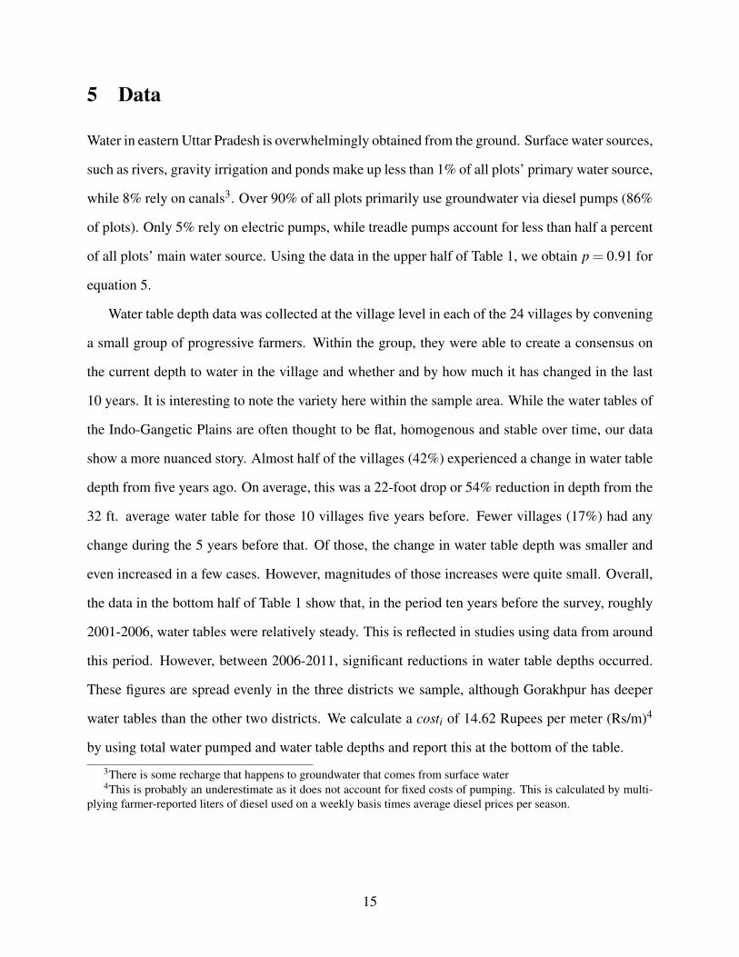
Water in eastern Uttar Pradesh is overwhelmingly obtained from the ground. Surface water sources,
such as rivers, gravity irrigation and ponds make up less than 1% of all plots’ primary water source,
while 8% rely on canals3. Over 90% of all plots primarily use groundwater via diesel pumps (86%
of plots). Only 5% rely on electric pumps, while treadle pumps account for less than half a percent
of all plots’ main water source. Using the data in the upper half of Table 1, we obtain p = 0.91 for
equation 5.
Water table depth data was collected at the village level in each of the 24 villages by convening
a small group of progressive farmers. Within the group, they were able to create a consensus on
the current depth to water in the village and whether and by how much it has changed in the last
10 years. It is interesting to note the variety here within the sample area. While the water tables of
the Indo-Gangetic Plains are often thought to be flat, homogenous and stable over time, our data
show a more nuanced story. Almost half of the villages (42%) experienced a change in water table
depth from five years ago. On average, this was a 22-foot drop or 54% reduction in depth from the
32 ft. average water table for those 10 villages five years before. Fewer villages (17%) had any
change during the 5 years before that. Of those, the change in water table depth was smaller and
even increased in a few cases. However, magnitudes of those increases were quite small. Overall,
the data in the bottom half of Table 1 show that, in the period ten years before the survey, roughly
2001-2006, water tables were relatively steady. This is reflected in studies using data from around
this period. However, between 2006-2011, significant reductions in water table depths occurred.
These figures are spread evenly in the three districts we sample, although Gorakhpur has deeper
water tables than the other two districts. We calculate a costi of 14.62 Rupees per meter (Rs/m)4
by using total water pumped and water table depths and report this at the bottom of the table.
3There is some recharge that happens to groundwater that comes from surface water4This is probably an underestimate as it does not account for fixed costs of pumping. This is calculated by multi-
plying farmer-reported liters of diesel used on a weekly basis times average diesel prices per season.
15
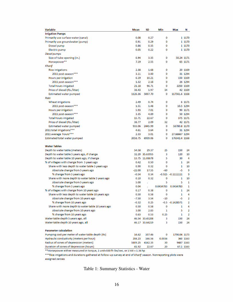
Table 1: Summary Statistics - Water
16

Rainfall during the kharif and rabi seasons of 2010-2011–the year leading up to the household
survey–was more erratic than over the 5-year average (see Figure ). The dry planting periods
of April and May 2010 saw about 24 inches of rain total, compared to an average of nearly 73
inches for those two months between 2008-2012. However, the monsoon period of July-September
produced 50% more rain than normal in this area. The rabi season then produced almost no rain,
only a sixth of the average.
Figure 7: Rainfall during 2010-2011 in eastern UP was erratic compared to the five-year average
Typical ranges of hydraulic conductivity for the different soils found in eastern Uttar Pradesh
are between 0.1 and 0.000001 meters per second for the soils in EUP and can go up to 1 x 10^-9
for pure clay elsewhere. Converting to meters per hour produces a range for soils in our sample
between 0.0036 to 360 m/hr. The soil types in this area are Balvi domat (sandy loam), Kali (black),
Chikni domat (clay loam), and Martika (clay), the first three of which are mostly found in lowland
areas and generally have more moisture and clod formation. Balvi domat, by contrast, is a light soil
that erodes quickly and leads to uneven fields because of continuous need for tillage and puddling
17

in agricultural preparation. There was more demand for laser land leveling on lands for plots with
this soil.
Figure (8) shows how the soils in this area of India fall between the most porous, sandy type
and the hardest, most dense clay variety. The majority of plots, 51%, consist of Balvi domat,
which, because of its light consistency, leads to bigger but shorter duration cones of depression, as
well as higher rates of hydraulic conductivity. Over a third of plots have either clay or clay loam,
as shown in Table 2. Pure clay plots, on which hydraulic conductivity is the lowest and cones of
depression the smallest and longest in duration, do not make up much of the sample, at only 7%.
The climate of UP suggests that black soils may contain up to 30% sand, more than 40% clay and
15-45% silt (Bhattacharyya et al. 2007). The clay in kali soil can be further broken down into a
majority coarse clay, as opposed to fine. This places it roughly in the middle of the soil triangle
and in the same neighborhood of weight and conductivity of clay loam. We use lower values of K
that represent differences in rates of hydraulic conductivity for these soil types and combine all of
these in proportion to their share in the sample.
Figure 8: This triangle shows the percentage of clay, silt and sand in various soil types. Sandy loammust be at least half sand and no more than 20% clay and 30% silt. Clay loam is lighter than clayand, thus, leads to larger-radius and shorter-duration cones of depression during pumping. Source:http://www.oneplan.org/Water/soil-triangle.asp
18

As mentioned earlier, the radius of cones of depression depends on hydraulic conductivity and
volume pumped5. We obtain values of these for each soil type/hydraulic conductivity combination,
as well as for durations of the cones. We generate values of cone duration per meter for each soil
type and multiply it by the radius when calculating the duration of cone. Duration per meter will be
highest for clay soils but clay soils allow the least amount of radial expansion. Further, it represents
only 7% of the sample.
Table 2: Summary Statistics - Farms
5This also depends the thickness of the unconfined aquifer with a maximum saturated thickness equal to the min-imum depth to water table (Maréchal et al 2011). Thus, when calculating estimated radii, we need use a value ofthickness not exceeding the depth to water table.
19
Because it has been shown that laser land leveling reduces water pumped by 26% (Lybbert
et al., 2013), we set β = 26. Here, we additionally estimate impacts of LLL on number of irriga-
tions and reduced duration of irrigations. The results in Tables 3 and 4 show that laser land leveling
additionally reduces the chance that plots level simultaneously through its effect of reducing the
duration of irrigations but not on total irrigations. Farmers spend up to 1.8 fewer hours pumping
water per year when their field is laser land leveled. Because the actual mean duration of pumping
in 2011 was 2.3 hours, this amounts to a 43-77% decrease in pumping duration. Thus, we start
with δ =−43 and then consider a range of δ ∈ (−77,−43), while setting γ = 1 so that there is no
multiplier effect via number of irrigations.
Table 3: Effect of Laser Land Leveling on Duration of Irrigations
20

Table 4: Effect of Laser Land Leveling on Number of Irrigations
Finally, the change in water table depth in equation 5 is the difference between equations 6 and
7. For each plot that is leveled, we generate plot-level water pumped, pumpi, as the product of tube
opening, horsepower of pump and total irrigation hours and report this in Table 1 (2,059 liters on
average per year). Total village acres leveled, Lv, is our variable during our simulations, as is the
number of farmers leveling as captured by the indicator in equation 7. In eastern Uttar Pradesh, 168
plots initially used LLL after our intervention, resulting in 1.3 acres leveled per leveling household,
6.4 acres per village, 126 acres in the sample, and 122 farmers total. These statistics are shown at
the bottom of Table 2.
6 Results
In the first specification, we assume all farmers are identical. They pump the same amount of
water on average and generate the same cones of depression in both size and duration. The same
21
distribution of soil within our sample applies uniformly within each village. Water wells are also
uniformly spaced 100 meters apart.
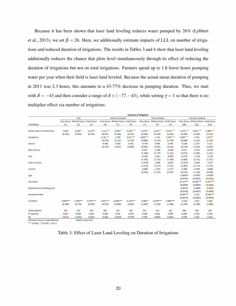
Using initial levels of adoption equal to those actually observed in eastern Uttar Pradesh, we
generate a ratio of impacts on water table depth between surface and ground of roughly 25:75. To
achieve this, we measure hydraulic conductivity in meters per minute and specify e = 5 in equation
7. The second term in this equation equals -1.88 meters and the third term -5.1, while the first term
cancels out when differencing from equation (6). Thus, the change in effective water table, ∆w,
equals 7 meters in our sample area, with a diesel cost savings to nonadopters of laser land leveling
of Rs. 1865.
We now use this initial equation to measure changes from increasing both the acres and number
of farmers involved with leveling. Doubling the number of farmers alone works through the indica-
tor function in the third term of the equation. Assuming all other parameters remain constant, this
simply doubles the effect on water table depth via cones to -10.2, bringing the total effect to -12.1
and a financial savings of Rs. 3230. Doubling area leveled only without changing the number of
farmers only impacts water tables through hydraulic conductivity, resulting in
From a practical perspective, one would more likely intervene at the farmer level in order to
increase leveling, not decide on amount of area targeted first. Nevertheless, if this ratio between
farmers leveling and area leveled is linear, then doubling the number of farmers adopting within a
village also doubles the area. This can simultaneously impact leveling through the surface. This is
captured in the additively separable form of equation 7.
Laser land leveling’s impact on duration of irrigation impacts water table depths and diesel
costs to nonadopters through cones only, specifically, via δ . We use the range of δ estimated
earlier and report the remaining results in Table (5).
22
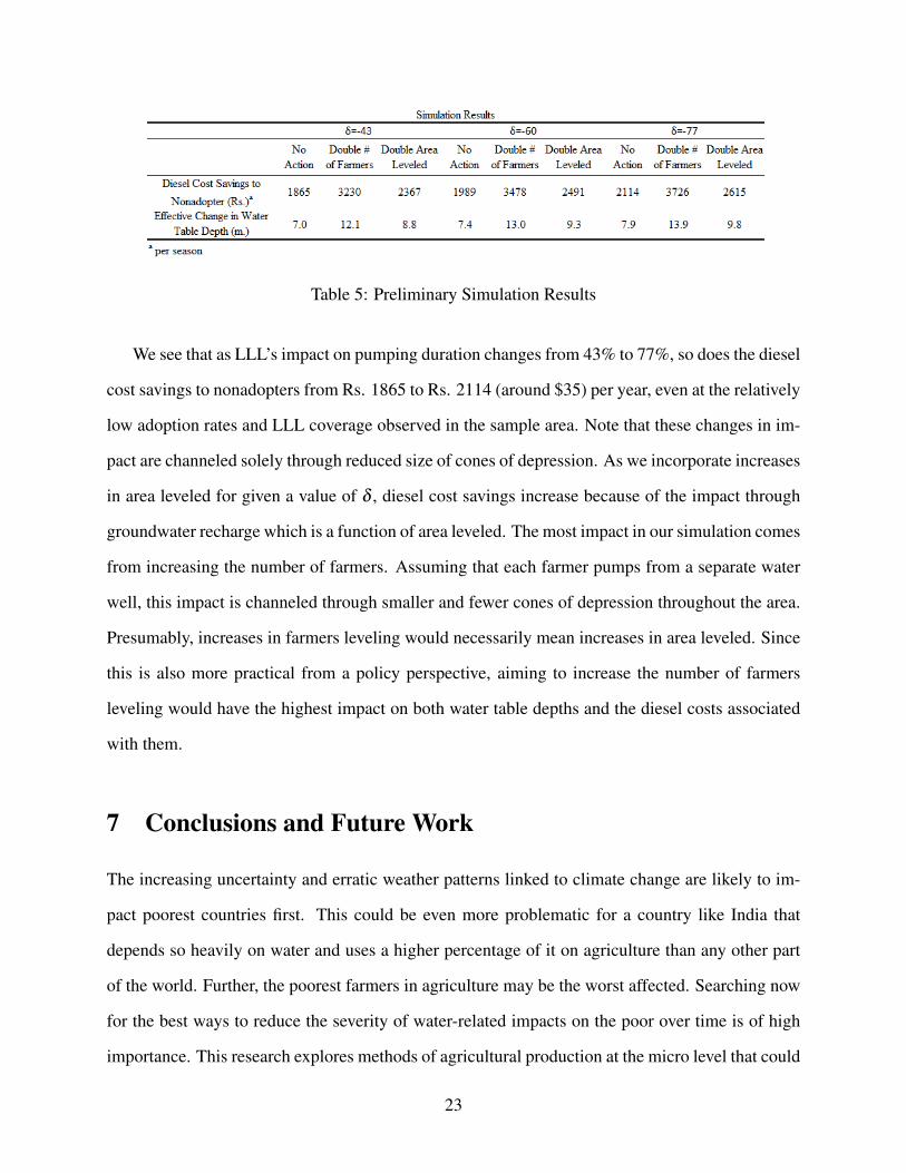
Table 5: Preliminary Simulation Results
We see that as LLL’s impact on pumping duration changes from 43% to 77%, so does the diesel
cost savings to nonadopters from Rs. 1865 to Rs. 2114 (around $35) per year, even at the relatively
low adoption rates and LLL coverage observed in the sample area. Note that these changes in im-
pact are channeled solely through reduced size of cones of depression. As we incorporate increases
in area leveled for given a value of δ , diesel cost savings increase because of the impact through
groundwater recharge which is a function of area leveled. The most impact in our simulation comes
from increasing the number of farmers. Assuming that each farmer pumps from a separate water
well, this impact is channeled through smaller and fewer cones of depression throughout the area.
Presumably, increases in farmers leveling would necessarily mean increases in area leveled. Since
this is also more practical from a policy perspective, aiming to increase the number of farmers
leveling would have the highest impact on both water table depths and the diesel costs associated
with them.
7 Conclusions and Future Work
The increasing uncertainty and erratic weather patterns linked to climate change are likely to im-
pact poorest countries first. This could be even more problematic for a country like India that
depends so heavily on water and uses a higher percentage of it on agriculture than any other part
of the world. Further, the poorest farmers in agriculture may be the worst affected. Searching now
for the best ways to reduce the severity of water-related impacts on the poor over time is of high
importance. This research explores methods of agricultural production at the micro level that could
23
combine with national and international climate policies at a macro level to achieve this.
We find that, in addition to 26% decreases in private water usage due to adoption of laser land
leveling, significant public reductions in diesel fuel needed to pump water also accrue to non-
adopters. This expands the total number of benefactors to include nonadopters and also produces
a secondary environmental benefit to water table depletion rates in the form of less diesel con-
sumed. Estimates produced here are likely to be lower bounds on water savings because increases
in effective water table depths can simultaneously increase marginal water usage by decreasing
the de facto price of pumping, which is a function of water table depth and pump horsepower and
specifications. National or state governments interested in reducing poverty and increasing water
availability both now and for future generations may want to consider such resource conserving
technologies as a policy tool.
Moving forward, improved data on hydrological variables in both in EUP and around India can
improve both estimates provided here and their applicability to other hydro-ecological systems.
And improved precision in converting hydrological parameters into economic results can help
bridge the gap between the specifics of the land on which so many poor farmers depend and the
economic prosperity and opportunities that have been sorely lacking in many of these villages in
the past.
References
Lybbert, T.J., N. Magnan, D.J. Spielman, A. Bhargava, and K. Gulati. 2013. Targeting technol-
ogy to reduce poverty and conserve resources: Experimental delivery of laser land leveling to
farmers in Uttar Pradesh, India, vol. 1274. Intl Food Policy Res Inst.
Madani, K., and A. Dinar. 2012. “Non-cooperative institutions for sustainable common pool re-
source management: Application to groundwater.” Ecological Economics 74:34 – 45.
Ostrom, E. 1995. “The institutional analysis and development framework: An application to the
24

study of common-pool resources in sub-Saharan Africa.” In Bloomington, Indiana: Workshop
in Political Theory and Policy Analysis, Indiana University. vol. 10.
25