title of thesis: embedded strain sensor with power
TRANSCRIPT

ABSTRACT
Title of Thesis: EMBEDDED STRAIN SENSOR WITH POWER
SCAVENGING FROM BRIDGE VIBRATION
Ming Wang, Master of Science, 2004
Thesis directed by: Professor Peter C. ChangDepartment of Civil Engineering
The Objective of this thesis is to investigate an embedded strain sensor system with
power scavenged from highway bridge vibration for structure health monitoring. A power
scavenging scheme is developed to power the sensor system so as to eliminate the
dependence of batteries. Three mechanisms (PZT patch, cantilever beam and PZT
stacks/slugs) are described that are suitable for the remote sensor system to scavenge
mechanical energy at different locations in a bridge. Calculations and experiments are taken
to examine the feasibility of the idea, and predicted power generation is compared to
solar/light power. A scheme of an embedded strain sensor using resonant MEMS beam
structure is introduced along with the theoretical analysis and simulation. The last
consideration is the signal propagation attenuation in concrete. Measurements are taken to

determine the RF signal attenuation at 900 MHz range transmitted through a concrete slab.
Theoretical calculations are validated by experimental results.

EMBEDDED STRAIN SENSOR WITH POWER SCAVENGING
FROM BRIDGE VIBRATION
by
Ming Wang
Thesis submitted to the Faculty of the Graduate School of theUniversity of Maryland, College Park in partial fulfillment
of the requirements for the degree ofMaster of Science
2004
Advisory Committee:
Professor Peter C. Chang, ChairProfessor Chung C. FuProfessor Darryll Pines

©Copyright by
Ming Wang
2004

ii
Table of Contents
List of Figures............................................................................................................. iiiList of Tables ................................................................................................................vIntroduction ..................................................................................................................1
1.1 Power scavenging from highway bridge vibration.......................................31.2 Embedded beam-type strain sensor ..............................................................51.3 Signal attenuation in concrete ......................................................................5
Embedded Sensor System for Structural Health Monitoring .......................................8Power Scavenging from Highway Bridge Vibration..................................................11
3.1 Bridge Vibration.........................................................................................113.2.1 Piezoelectric Phenomenon..................................................................173.2.2 PZT Patch ...........................................................................................18
3.2.2.1 Power generation from truckload-induced strain ...........................213.2.2.2 Power generation from strain induced by free vibration ................24
3.2.3 Cantilever Beam with Tip Mass .........................................................263.2.4 PZT Stacks/Slugs................................................................................32
3.3 Energy Storage Consideration....................................................................363.4 Experimental Results..................................................................................363.5 Comparison to other forms of available energy .........................................39
Resonant Beam-type Strain Sensor ............................................................................424.1 Beam Vibration Analysis ...........................................................................434.2 ANSYS Simulation Result .........................................................................45
4.2.1 Beam with no pre-tension...................................................................464.2.2 Pre-tensioned MEMS Beam...............................................................47
4.3 Capacitance Excitement of the Beam Vibration ........................................484.4 Capacitance Detection of the Beam Resonant Frequency..........................494.5 Temperature Compensation........................................................................51
Measurement of Propagation Attenuation through Concrete .....................................535.1 Electromagnetic Wave Propagation ...........................................................53
5.1.1 Reflection and Transmission Coefficient ...........................................535.1.2 Penetration Depth ...............................................................................57
5.2 Dielectric Constant of Concrete .................................................................585.3 Experimental Set-up and Results................................................................59
Conclusion..................................................................................................................656.1 power scavenging from highway bridge vibration .....................................656.2 Embedded MEMS beam-type strain sensor ...............................................666.3 Propagation Attenuation through Concrete at 900 MHz............................67
References ..................................................................................................................68

iii
List of Figures
Figure 1.1 SG-Link node..……………………………..…………………....…….… 2 Figure 2.1 Block diagram of embedded sensor system................................................9Figure 3.1 Schematic drawing of girder bridge and truckload model ........................12Figure 3.2 Truckload model used in ANSYS.............................................................12Figure 3.3 Finite element mesh plot ...........................................................................13Figure 3.4 First four vibration mode shapes...............................................................14Figure 3.5 Dynamic displacement of girder, (a) vertical displacement at mid-span
and (b) vertical displacement at a point 2 feet from support ..............................15Figure 3.6 Dynamic strains at (a) mid-span and.........................................................16Figure 3.7 Piezoelectric sensor operation modes .......................................................18Figure 3.8 Strain changes of girder bottom at (a) mid-span and ................................20Figure 3.9 Vibration signals after filters (mid-span location) ....................................23Figure 3.10 Peak power output under different test resistance load...........................23Figure 3.11 Instantaneous power under 3.85M Ohms load........................................24Figure 3.12 Peak power output under different test resistance load (for high
frequency vibration) ...........................................................................................25Figure 3.13 Instantaneous power under 281 K Ohms load ........................................26Figure 3.14 Schematic drawing of cantilever beam with tip mass.............................28Figure 3.15 Schematic drawing of cantilever-type generator ....................................28Figure 3.16 Beam distortion y(t) at tip and strain in PZT layer .................................31Figure 3.17 Peak power output under different test resistance load...........................31Figure 3.18 Power estimation with different PZT layer thickness .............................32Figure 3.19 Vehicle-induced compressive impact stress on PZT stack. PZT stack
locates at the mid-span point on the top of interior girder. A two-axle truck moves on bridge with speed 60mile/hour...........................................................34
Figure 3.20 A multilayer stack under stress ...............................................................35Figure 3.21 Stress amplification scheme....................................................................35Figure 3.22 PZT stack array .......................................................................................35Figure 3.23 Parasitic patch on a free vibration beam .................................................38Figure 3.24 Experimental and estimated peak power output .....................................38Figure 3.25 Solar panel……………………………………………………………...39Figure 4.1 System for resonant beam strain sensor ....................................................43Figure 4.2 x and w axis set up for studying the beam vibration.................................43Figure 4.3 Schematic diagram of the vibrating MEMS beam....................................46Figure 4.4 MEMS beam resonant frequency response with the strain change...........47Figure 4.5 Schematic diagram of compensation beam structure................................52Figure 5.1 Electromagnetic wave propagates from medium1 to medium 2...............55Figure 5. 2 Schematic drawings of TE and TM waves ..............................................55Figure 5.3 [Loulizi, 2001] Concrete dielectric constants vs. frequency.....................59Figure 5.4 Schematic drawing of experiment setup ...................................................61Figure 5.5 Schematic drawing of helical antenna ......................................................61

iv
Figure 5.6 Transmitting of RF energy through different material. (a) Open space. (b) Wood wall board. (c) Concrete slab. (d) Metal plate. For all four plots, x-axis frequency vary from 0.5 to 1.5 GHz, with 50 MHz per grid. y-axis is the 20log10(EOUT/EIN), with 10 dB per grid. .............................................................63

v
List of Tables
Table 3.1 Modal analysis results ................................................................................13Table 3.2 PZT (PSI-5A-S4-ENH [Piezo Systems, Inc.]) material properties ............20Table 3.3 Power generation comparison ....................................................................40Table 3.4 Power obtained v.s. Power Demand...........................................................41Table 5.1 Attenuation taken at 917.5MHz .................................................................63

1
Chapter 1
Introduction
The traditional method to ensure the structural safety of civil infrastructure is to
do visual inspection regularly. This is a simple but ineffective means since the health of
structures can not be diagnosed adequately by its appearance alone. Critical
deteriorations or damages often occur inside the structure, for example the corrosion of
rebars in concrete. Corrosion initiation and growth are difficult to be perceived and
controlled. Research on structural health monitoring for civil infrastructures and
space/aircraft transportation system has experienced rapid growth in recent years. For
example, accelerometers are placed on a structure, and then the vibration of the structure
can be used to determine the condition of the structure. This is a global health
monitoring method by observing changes of dynamic properties of the structure. Local
monitoring method is to place sensors at some pre-determined hot spots where damage is
expected. Both global and local methods need to install sensors in the investigated
structure. Useful structural information (e.g.: strain/stress, acceleration, temperature etc.)
is then obtained by monitoring those sensors.
The traditional methods of communication between sensors and data collection
units rely on wire connections. However not only is the wiring a large number of sensors
costly, but also large bundles of wires from different parts of a structure are difficult to
manage and they are subjected to environmental deterioration. So, remote wireless
technology becomes an attractive means to establish communication between sensors
and a central unit.

2
The concept of wireless monitoring system was introduced in [Straser et al.,
1998], and a wireless modular monitoring system (WiMMS) [Lynch et al., 2000] was
then developed using economical and commercially available components for
implementing the wireless communication of sensor measurements in structures. A
WiMMS unit is powered by 3 groups of 6 AA alkaline batteries (18 total), which
provides up to 21 days in sleep mode and up to 11 hours for continuous operation [Straser
et al., 2000]. SG-Link™ Wireless Strain Gauge System [MicroStrain, Inc.] is a
commercially available product which combines full strain gauge conditioning with
micro datalogging transceiver system for fulfilling wireless strain monitoring. SG-Link
node, as shown in Figure 1.1, is powered by a 3.6 volt lithium ion AA size internal
battery which provides up to 230 hours of lifespan.
In this thesis, an
embedded sensor system
for structural health
monitoring of highway
bridges is described. This
sensor system employs a
power scavenging device
to harvest energy from the
bridge vibration so that the
dependence of batteries is
eliminated, and the lifespan of the sensor system is then increased. Strain information is
obtained by a vibrating beam-type stress sensor and the integrated transmitter sends
Figure 1.1 SG-Link node

3
those results back to a handheld monitor via radio frequency signals. This realizes the
operation of a wireless, self-powered and embedded sensor system for structural health
monitoring.
This thesis concentrates on three main aspects: power scavenging from highway
bridge vibration, embedded beam-type strain sensor and signal attenuation in concrete.
1.1 Power scavenging from highway bridge vibration
The capability of health monitoring system relies on the performance and
reliability of sensors. So sensors should be able to work in a sustained mode and do not
need to be replaced or repaired over the life of the structure. Embedded sensors are
recently considered as promising means. However, powering these sensor systems is a
significant problem since battery power offers only a limited life span, and battery
management is inconvenient and impractical. Self-powered sensors are attractive
because they allow the sensors to be tetherless. Moreover they make use of the energy
from the ambient environment which is usually dissipated as heat and radiation. The
harvested energy could be converted into a useful form upon the demand of sensors. The
ideal case is that the harvested power is sufficient to provide a constant power supply for
the sensor system. This depends on both the amount of power harvested from the
environment and the power consumption of the sensors. An alternative way is to store
the generated energy and give a power burst to the sensor system when power is needed.
Various approaches have been studied to convert and store energy from ambient
energy sources, including solar [Lee et al., 1995], [Warneke et al., 2002], human power
[Starner, 1996], radio frequency [Friedman et al., 1997], [Wu et al., 2001], [Jung et al.,
4
1999], thermal gradients [Glosch et al., 1999] and mechanical vibration [Williams et al.,
1997], [Meninger et al., 2001], [Amirtharajah et al., 1998], [Glynne-Jones et al., 2001],
[El-hami et al., 2001], [Shearwood et al., 1997].
A successful example of power scavenging is the “parasitic piezoelectric shoe”
[Shenck et al., 2001] developed by the MIT Media Laboratory. The “piezoelectric” shoe
utilizes PZT uniform and polyvinylidene fluoride (PVDF) stave mounted under an insole
as the power generating element; an average of 1.3 to 8mW of power was collected at a
0.9 Hz walking pace. The harvested energy successfully powered an RFID tag system
and transmitted an identification signal to local surroundings. Similarly researchers in
Sandia National Laboratory have developed piezoelectric-based self-powered sensor tags
and proposed the idea to use the sensor tags to monitor the state-of-health of structures
[Pfeifer et al., 2001]. The design of a MEMS transducer system that converts ambient
mechanical vibration into electrical energy through the use of a variable capacitor was
presented in [Meninger et al., 2001]. The feasibility of operating a digital system from
power generated through a vibration-based power generator is demonstrated in
[Amirtharajah et al., 1998], in which an integrated chip was designed and tested. A thick-
film piezoelectric microgenerator and vibration-based electromechamical power
generator were introduced and experimental setups described in [Glynne-Jones et al.,
2001] and [El-hami et al., 2001], respectively.
With the development of vibration-to-electric energy conversion technology,
researchers have begun to think of using energy harvesting means to power the sensors
installed in highway bridges, such as accelerometers, strain gages, thermometers,
anemometers, and even video monitors. [Williams et al., 1997] presented a feasibility

5
study of a vibration-to-electric generator designed to generate power from bridge
vibration. However it is not clear how much power can be harvested in a highway
bridge. This thesis attempts to estimate the power that can be generated quantitatively.
1.2 Embedded beam-type strain sensor
The most common strain sensors are surface mounted resistance strain gauges.
Vibrating wire spot-weldable strain gauge [Ace Instrument Co., Ltd.] is designed to be
embedded in reinforced concrete to detect strain in concrete or strain in steel rebars. This
kind of embedded strain gauge needs shielded cables to transmit the signals out. So the
amount of such sensors in a structure has to be restricted in order not to influence the
performance of the structure.
In this thesis, a MEMS beam-type strain sensor which can be either mounted on
the surface or embedded inside of a structure is investigated. The device is a beam fixed
at both ends for which the resonant frequency is determined by its axial strain which is
related to its resonant frequency. This kind of strain sensor is more stable than the
traditional resistance strain gauges. The linear relationship between strain and frequency
is studied by simulating a beam-type device under different axial stresses. The
capacitance excitement and detection technologies are also investigated.
1.3 Signal attenuation in concrete
Once an embedded sensor is installed in a bridge, and it is powered by the means
of energy scavenging, it is necessary to know if the harvested power is sufficient for the
sensor’s demand. The attenuation of radio frequency energy is ineluctable when radio

6
frequency wave transmits through concrete to reach the embedded sensors or when the
sensors transmit signals out. For a scheme of power scavenging, the energy harvested by
the sensors should be sufficient to complete sensing, data processing and data out-
transmitting. If the propagation attenuation is too big, the signal strength sent from
transmitter has to be high enough, but sometimes this requirement is infeasible when the
power supply is limited. Some empirical and theoretical models have been developed to
investigate the influence of construction material such as concrete wall, wood or steel
door, windows and so on in modern office building environment [Lafortune et al., 1990],
[Honcharenko et al., 1992], [Honcharenko et al., 1993], [Seidel et al., 1994], [ Lawton et
al., 1994] and [Lawton et al., 1999]. In order to determine the depth at which an
embedded sensor can possibly be placed, the attenuation of RF energy through concrete
needs to be studied.
In this thesis, chapter 2 introduces the embedded sensor system for structural
health monitoring. Chapter 3 describes the simulation of the traffic-induced vibration of
a girder bridge model and then investigates three approaches for piezoelectric-based
power scavenging based on the simulation results. Power storage considerations and
some experimental results are also discussed in this chapter, and the expected power
generation is compared to solar power and the power demand estimation of the
embedded strains sensor system. In Chapter 4, a resonant MEMS beam strain sensor is
studied. The capacitance excitement and detection technologies are also discussed. In
chapter 5, the measurement of propagation attenuation through concrete at 900 MHz
range was presented. Chapter 6 concluded this thesis with summary of results and
insights and indicates areas of future research.

7

8
Chapter 2
Embedded Sensor System for Structural Health Monitoring
Strain sensors often need to be embedded inside the structure to measure local
strain of the structural components such as reinforcement steel. The goal of this research
is to investigate the possibility of using an embedded sensor system for health monitoring
of highway bridges. The sensor system consists of a sensor module, a power scavenging
module, a system controller module and a transceiver module. The sensor module takes
measurements of structural information such as strain. The power scavenging module is
to harvest energy from ambient sources such as highway bridge vibration, and the
harvested energy is stored in a power storage device. This module provides the power
demand for the sensor system. The system controller module controls the operation
modes of the system including sleeping mode and working mode. The transceiver module
has two functions: receiving command signals from a handheld monitor and transmitting
information of structures back to the handheld monitor. The system block diagram is
shown in Figure 2.1.

9
Figure 2.1 Block diagram of embedded sensor system
Without commands from handheld monitor, the sensor system is in “sleeping”
status. The power scavenging module provides a constant power for receiver and system
controller module to be sustained in a “waiting” status. When the receiver gets a “wake
up” command signal from the handheld monitor, the system controller module gives
“working” commands to the sensor and power scavenging modules. The power
scavenging module provides sufficient power for the demand of the sensor module and
the transceiver module by discharging the power storage device. The embedded sensor
starts to collect structure information and the transmitter sends those results back to the
handheld monitor. When the handheld monitor obtains the expected information, it sends
a “sleeping” command out, and the sensor system goes to “sleeping” mode. The collected
information is either stored in the handheld device or sent to a central unit for advanced
analysis.
The sensor system has three main advantages:
Hand held monitor
Transceiver Module
Receiver
Transmitter
Power Scavenging Module
Power scavenging device
Power storage device
comm
and
Structure Inform
ation
Sensor Module
Embedded sensor
System Controller Module
Power supply
Power supply
Power supply
“working/sleeping”
“working/
sleeping”
Structure Inform
ation
comm
and

10
� Wireless
� Embedded in structures
� Self-powered
Since the operation of the embedded sensor system relies on the power supplied
by the power scavenging module, Chapter 3 gives the estimation of expected power
generation from bridge vibration, and compares it to solar power. Finally, the power
demand estimation of the sensor system is also given for comparison.
Traditional resistance strain gauges drift significantly in even short periods of
time, so they are not suitable for the purpose of long-term monitoring. Chapter 4
introduces a MEMS resonant beam-type strain sensor which is more stable, and it can be
embedded and it is wireless. Excitation and detection methods are also investigated.
Since the embedded sensor system is designed to be placed inside of a structure,
the signal attenuation has to be considered when the transceiver module sends a signal
out or receives a signal from handheld monitor. Chapter 5 investigates the signal
attenuation problem by doing measurement.

11
Chapter 3
Power Scavenging from Highway Bridge Vibration
3.1 Bridge Vibration
Highway bridges vibrate considerably because of vehicle loading and wind. This
mechanical energy is dissipated to the environment as heat. In order to determine the
amount of mechanical energy that can be harvested, a typical T-shape girder bridge
model was developed using ANSYS [ANSYS, Inc., 1998] and the dynamic
characteristics of the bridge were obtained by modeling the passage of trucks.
A typical single span bridge is assumed. It is supported by three T-shape girders,
and it is assumed to be simply supported at both ends. The traffic on the bridge consists
of two lanes with a single lane in each direction as shown in Figure 1. The span length, L,
is 88 feet and the deck thickness is 7 inches, which represents a typical highway overpass
bridge. The height of the T-shape girder is 65 inches and the thickness is 8 inches. The
span space, S, is 10 feet.
The truck wheel load is considered as a three-axle truck (36KN-142KN-142KN)
as described in AASHTO Standard (HS20-44 Loading). Figure 3.2 shows the truck
loading model. Assume the trucks speed to be 96 km/hour (60 mph). At this speed a
wheel takes approximately 1 second to cross this single span.

12
Figure 3.1 Schematic drawing of girder bridge and truckload model
Figure 3.2 Truckload model used in ANSYS
A four-node isoparametric shell (Shell 63) [ANSYS, Inc., 1998] is chosen as the
structure element in ANSYS. Both modal and transient dynamic analyses were
performed. Figure 3.3 shows the finite element mesh used.
Traffic
Direction
Traffic
Direction
L
S
S
T Girder section
16K
4K
16K
16K 16K
4K
20 feet14 feet
6 feet
13
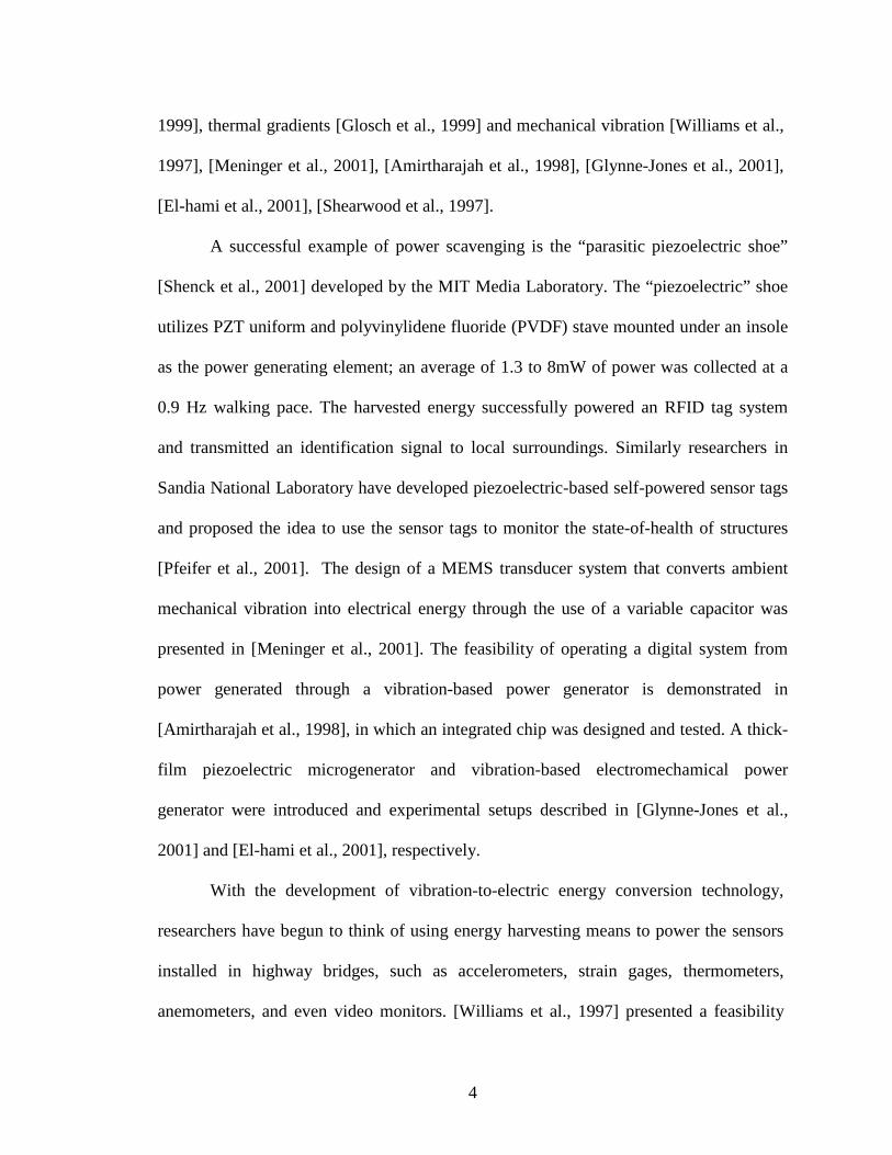
The modal analysis shows that the natural frequency of the first mode is 8.51 Hz.
Table 3.1 shows the first five modes of vibration. Figure 3.4 gives the first four vibration
mode shapes.
Transient dynamic analysis is performed to determine the dynamic response of
the structure under the action of the moving truck. The dynamic displacement of an
interior girder was obtained from the transient dynamic analysis. Figure 3.5 (a) and (b)
shows the time-history displacement at the mid-span point and a point 2 feet from the left
support, respectively. Figure 3.6 (a) and (b) show their dynamic strains.
Table 3.1 Modal analysis results
Figure 3.3 Finite element mesh plot
1st mode 2nd mode 3rd mode 4th mode 5th mode
8.51Hz 8.56Hz 12.14Hz 17.71Hz 19.35Hz

14
Figure 3.4 First four vibration mode shapes

15
0 1 2 3 4 5 6-5.400
-5.200
-5.000
-4.800
-4.600
-4.400
-4.200
Dis
plac
emen
t (m
m)
Time (t)
(a)
(b)
Figure 3.5 Dynamic displacement of girder, (a) vertical displacement at mid-span and (b) vertical displacement at a point 2 feet from support
0 1 2 3 4 5 6-1.200
-1.000
-0.800
-0.600
-0.400
-0.200
0.000
Dis
plac
emen
t (m
m)
Time (s)

16
(a)
(b)Figure 3.6 Dynamic strains at (a) mid-span and
(b) a point 2 feet from support
These results show that the dynamic responses consist of two parts. One part
corresponds to the bridge’s free vibration which corresponds to the higher frequency
0 1 2 3 4
85
90
95
100
105
110
115
120
Str
ain
(10
-6
m/m
)
T im e (s)
0 1 2 3 4
21 0
21 5
22 0
22 5
23 0
23 5
24 0
24 5
Str
ain
(10
-6
m/m
)
T im e (s )

17
signals (around 8 Hz), and the other part corresponds to the truckload-induced vibration
which appears as the higher amplitude signal with lower frequency (around 0.8 Hz).
3.2 Approaches for Power Scavenging
The idea of energy scavenging here is to employ a piezoelectric structure as the
power generation element. Piezoelectric materials generate an electricity when subjected
to a mechanical deformation; and vice versa. The piezoelectric materials such as PZT
(lead zirconate titanate), ZnO, Quartz, PVDF (polyvinylidene fluoride) etc. have been
widely used as sensors and actuators. In [Weinberg, 1999] the solutions of working
equations for a piezoelectric beam are derived.
In this thesis, three types of approaches are studied: patch, cantilevered beam,
and stacks/slugs. They are suitable for harvesting different kinds of mechanical energy in
a bridge: structural strain, vibration, and impact compression.
3.2.1 Piezoelectric Phenomenon
Piezoelectric phenomenon was first discovered in 1880s by Pierre and Jacque
Curie. They found that some crystalline materials generate a voltage when compressed
(generator effect) and change shape when an electric field is applied (motor effect).
Although some natural materials (eg: quatz) are found to show piezoelectric effects,
most modern piezoelectric devices are made with artificial polycrystalline ceramics such
as PZT (lead zirconate titanate), which is considered in this thesis. Piezoelectric
properties are directionally dependent. Figure 3.7 shows the 33 and 31 operation modes
under generator effect. P denotes the polarization direction of the PZT material.

18
Figure 3.7 Piezoelectric sensor operation modes
The piezoelectric behavior can be described by the following equations:
ij ijD d X Eε= + (3.1a)
i ij iS sX d E= + (3.1b)
The index i indicates that the electrodes are perpendicular to axis i, and index j
indicates that the piezoelectric induced strain or the applied stress is in the direction j. D
is electrical displacement along polarization axis, and S is strain. dij is defined as
piezoelectric strain coefficient. ε is the dielectric constant of the material. E is the electric
field generated between electrodes. X is mechanical stress developed in piezoelectric
material. s is mechanical compliance in a constant electrical field. Equation 3.1a reflects
the generator effect and equation 3.1b reflects the motor effect.
3.2.2 PZT Patch
The patch configuration is the most direct and simple means to convert bridge
vibration into power. PZT patches can be placed on the surface of girders, usually on top
+-
P
F
F
+-P
FF
(a) 33 mode
3
1
2(b) 31 mode

19
of a flange or on the bottom of a slab, where the strain change is high relative to other
locations. At these locations, the PZT patches are subjected to stress changes due to
traffic loads. If the bond between the PZT patch and concrete transfers the deflection
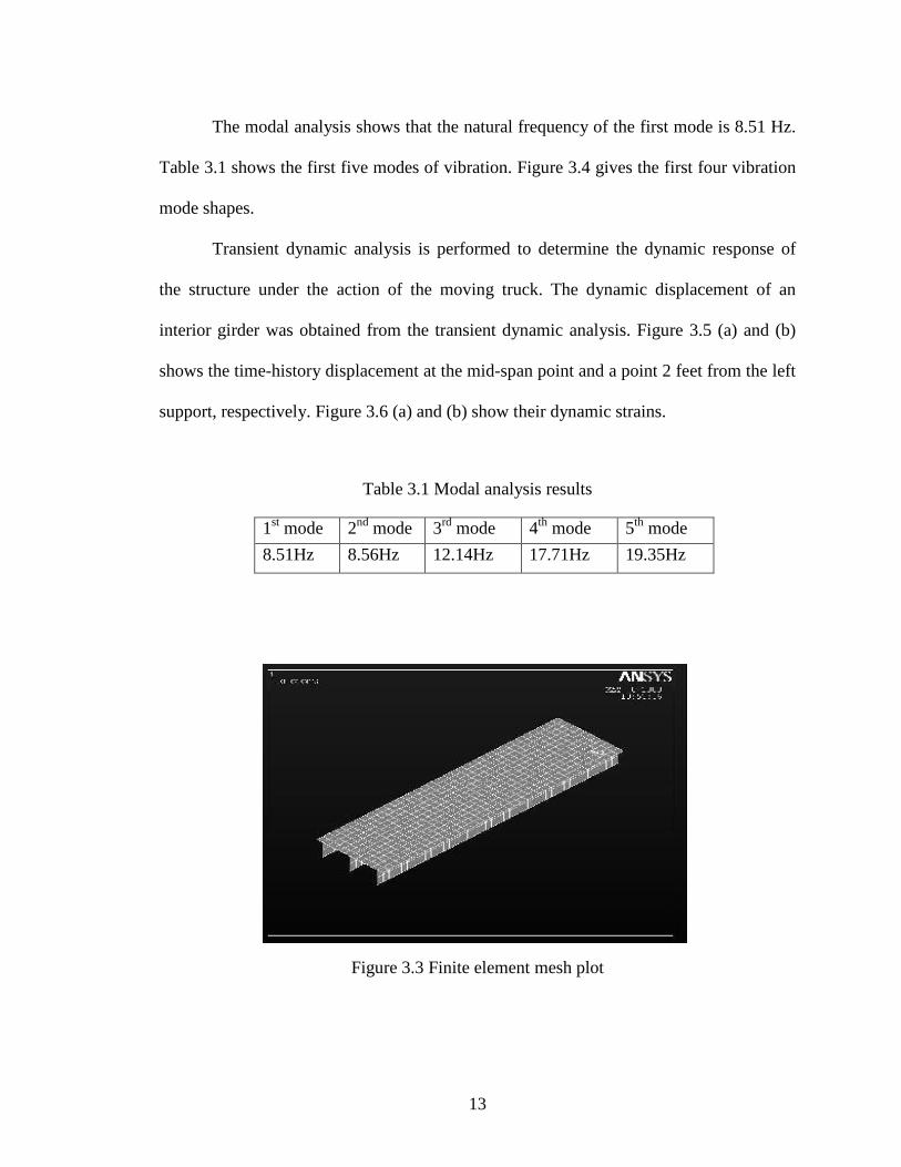
perfectly, the attached PZT patch has the same strain as the girder. Figure 3.8 (a) and (b)
show the strain change at the mid-span point on the bottom of girder and at the point
close to the support, respectively. The strain change in the PZT patch can be divided into
two parts: (1) traffic-induced strain and (2) free vibration strain. The traffic-induced
output has the properties of high amplitude but low frequency (26 micro strain and 0.77
Hz). The free vibration output has the properties of low amplitude but relatively high
frequency (4 micro strain and 8 Hz). The total power harvested by the PZT patches is
from the combination of these two vibration sources. Here a low-pass filter is used to
obtain the truck-induced vibration and a high-pass filter used to obtain the free vibration.
Then the power generation from these two vibration sources is calculated. Figure 3.9
shows the vibration signals after the filters.
If a 10cm×10cm×0.2cm PZT patch with mechanical and piezoelectric properties
shown in Table 3.2 is used, the harvested power can be estimated.
20
Table 3.2 PZT (PSI-5A-S4-ENH [Piezo Systems, Inc.]) material properties
(a)
(b)Figure 3.8 Strain changes of girder bottom at (a) mid-span and
(b) the point which is 2 feet to the left support
0 1 2 3 4
-5
0
5
10
15
20
25
30
Str
ain
chan
ge (
10
-
6 m
/m)
T im e (s)
d31
(m/volts)g31
(volt⋅m/N)εεεε3 k31 ρ
(Kg/m)E11
(N/m2)νννν
-190E-12 -11.6E-3 1800 0.32 7800 6.6E10 0.31
d31: piezoelectric strain coefficientg31: piezoelectric voltage coefficientε3: relative dielectric constant between poling electrodesk31: coupling coefficientρ: densityE11: elastic modulus in longitude ν: Poisson’s ratio
0 1 2 3 4
-5
0
5
10
15
20
25
30
Str
ain
chan
ge (
10
-6
m/m
)
Time (s)

21
3.2.2.1 Power generation from truckload-induced strain
This part of the time-history of strain change can be considered as a periodic
signal with frequencies around 0.5 Hz which is shown in Figure 3.9. The generated open
circuit voltage from the PZT patch can be written in terms of strain:
11 31open sV E g Tε= (3.2)
where εS is the longitudinal strain of the patch. T is the thickness of the PZT ceramic
layer.
From Figure 3.9, the maximum strain of the truck-induced vibration εs=21 micro
strain. Substituting it into (3.2), the maximum open circuit voltage is approximately 31.5
volts. Then the average energy generated in the PZT patch can be calculated based on the
peak voltage output:
2
2
1CVEe =
(3.3)
C is the capacitance of the PZT patch which is determined by
T
AC 30εε= (3.4)
A is the surface area of the electrode. In this case, A is equal to 100 cm2. ε3 is the relative
dielectric constant between poling electrodes and ε0 is the permittivity of vacuum.
(ε0=8.85×10⁻¹² farads/m)
From (3.4) the capacitance of the single PZT patch is about 80 nF. The available
energy then is calculated from (3.3):
JJvoltsFaradE e µ40100.4)5.31(100.82
1 528 =×=⋅×⋅= −−

22
The average available power in the 0.5Hz vibration is then:
52 2 0.5 4.0 10 40e eP f E Hz J Wµ−= × × = × × × =
f is frequency in Hz, and f is equal to 0.5Hz in this case. The area of the PZT
patch is 100cm2. So the power density is about 0.4µW/cm2.
The output power can also be determined by connecting a test resistance to the
patch device. The output power can be written: [Kendall, 1998]
211 31
2
( )
(1 ( ) )S
o
A E d RP
CR
ε ωω=
+(3.5)
where ω=2πf, and R is the test resistance.
If the maximum strain from Figure 3.9 (εs=21 micro strain) is substituted into to
(3.5), the peak power output can be obtained at an optimized test resistance. Figure 3.10
illustrates the peak power output versus test resistance, and it shows that the peak power
is around 124 µW at 3850 K Ohms.
If the optimized test resistance (R=3850 K Ohms) is substituted into (3.5), and use
the time-history strain change to replace εs, the instantaneous power can be obtained, and
is shown in Figure 3.11. The average power output is about 33 µW, which is close to 40
µW estimated by equations 3.3 and 3.4.

23
Figure 3.9 Vibration signals after filters (mid-span location)
1000 2000 3000 4000 5000 6000 7000 800070
80
90
100
110
120
130
Pea
k po
wer
out
put (
mic
ro W
atts
)
Test resistance (K Ohms)
Figure 3.10 Peak power output under different test resistance load
(for low frequency vibtation)
0 1 2 3 4
-5
0
5
1 0
1 5
2 0 lo w fre q u e n c y v ib ra tio n h ig h fre q u e n c y v ib ra tio n
Str
ain
Cha
nge
(10
-
6 m
/m)
T im e (s )

24
Figure 3.11 Instantaneous power under 3.85M Ohms load
(for low frequency vibration)
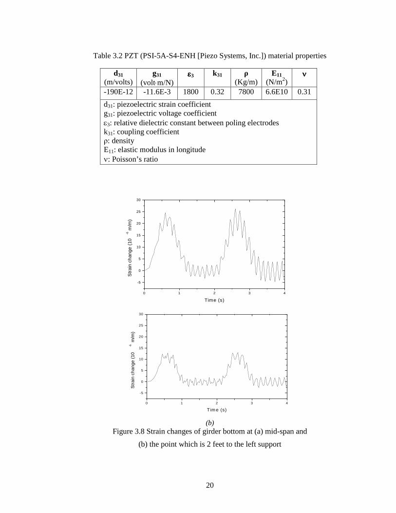
3.2.2.2 Power generation from strain induced by free vibration
The part of free vibration can be considered as a periodic signal with frequency
8.51 Hz shown in Figure 3.9. Following the same procedure as described in section
3.2.2.1, the PZT single patch generates a peak power of about 100 µW at 281 K ohms as
shown in Figure 3.12, and an average power of 22 µW as shown in Figure 3.13.
The results show that both low frequency and high frequency vibrations have
contributions to the power generation. Under optimized resistive loads, the total available
power from the PZT device is around 55 µW. If the PZT patch is placed on the bottom of
the interior girder at 1/4 span, the total available power output is around 25 µW.
The harvested power is related to the size of the PZT patch. Making the single
patch thicker will increase the power output. A thick PZT patch is commercially
0 1 2 3 4
0
20
40
60
80
100
120
140
Average Power
Pow
er (
mic
ro W
atts
)
Time (s)
25
available. For example, Morgan Electro Ceramics Ltd. supplies PZT sheets with
thickness ranging from 0.2mm to 15mm [Morgan Electro Ceramics].
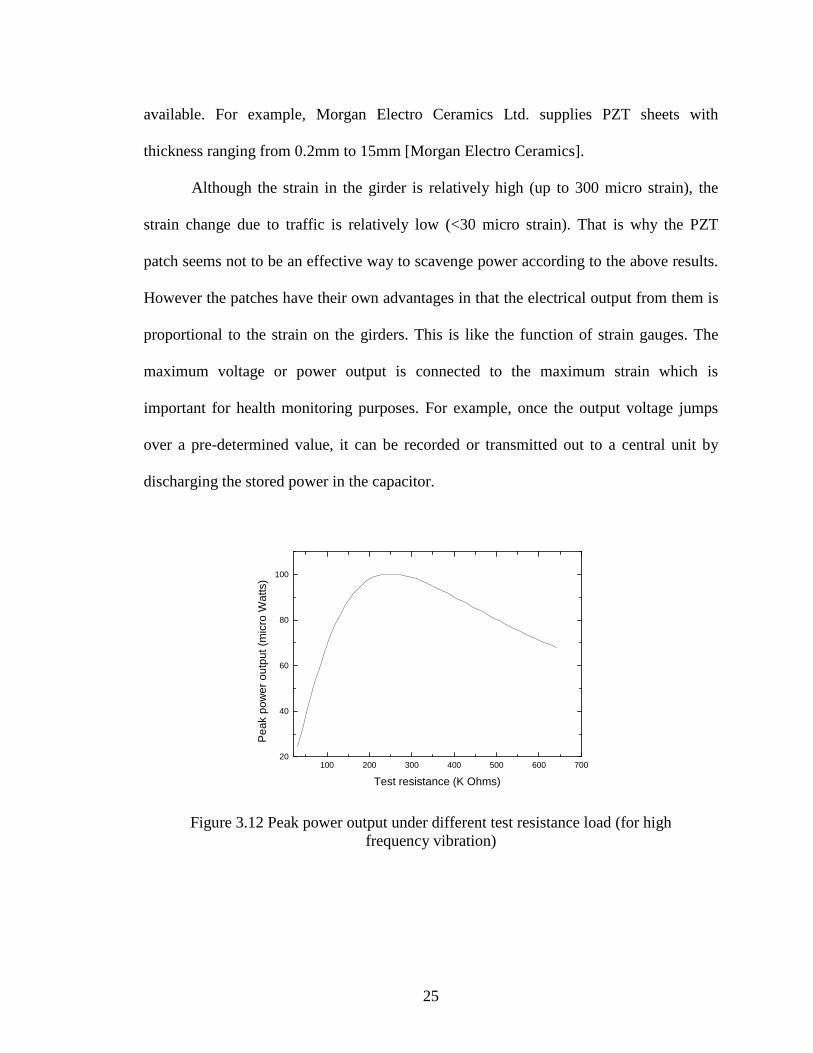
Although the strain in the girder is relatively high (up to 300 micro strain), the
strain change due to traffic is relatively low (<30 micro strain). That is why the PZT
patch seems not to be an effective way to scavenge power according to the above results.
However the patches have their own advantages in that the electrical output from them is
proportional to the strain on the girders. This is like the function of strain gauges. The
maximum voltage or power output is connected to the maximum strain which is
important for health monitoring purposes. For example, once the output voltage jumps
over a pre-determined value, it can be recorded or transmitted out to a central unit by
discharging the stored power in the capacitor.
Figure 3.12 Peak power output under different test resistance load (for high frequency vibration)
100 200 300 400 500 600 70020
40
60
80
100
Pea
k po
wer
out
put (
mic
ro W
atts
)
Test resistance (K Ohms)

26
Figure 3.13 Instantaneous power under 281 K Ohms load
(for high frequency vibration)
3.2.3 Cantilever Beam with Tip Mass
Figure 3.14 (a) is the schematic drawing of a cantilever beam structure with a tip
mass. The tip mass changes the natural frequency of the beam structure.
The model of the beam structure can be simplified since the weight of the beam is
small enough to be neglected compared to the tip mass. Figure 3.14 (b) and (c) show that
the clamped end is subject to a motion u(t), and y(t) is the displacement of the free end.
The equilibrium equation of the beam system is:
( )my cy ky mu P t+ + = − =�� � �� (3.6)
m is the mass at the free end; c is the mechanical damping coefficient and k is the
stiffness coefficient.
0 1 2 3 4
0
20
40
60
80
100
Average power
Pow
er (
mic
ro W
atts
)
Time (s)
27
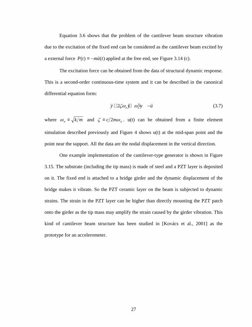
Equation 3.6 shows that the problem of the cantilever beam structure vibration
due to the excitation of the fixed end can be considered as the cantilever beam excited by
a external force )()( tumtP ��−= applied at the free end, see Figure 3.14 (c).
The excitation force can be obtained from the data of structural dynamic response.
This is a second-order continuous-time system and it can be described in the canonical
differential equation form:
22 n ny y y uζω ω+ + = −�� � �� (3.7)
where mkn =ω and nmc ωζ 2= . u(t) can be obtained from a finite element
simulation described previously and Figure 4 shows u(t) at the mid-span point and the
point near the support. All the data are the nodal displacement in the vertical direction.
One example implementation of the cantilever-type generator is shown in Figure
3.15. The substrate (including the tip mass) is made of steel and a PZT layer is deposited
on it. The fixed end is attached to a bridge girder and the dynamic displacement of the
bridge makes it vibrate. So the PZT ceramic layer on the beam is subjected to dynamic
strains. The strain in the PZT layer can be higher than directly mounting the PZT patch
onto the girder as the tip mass may amplify the strain caused by the girder vibration. This
kind of cantilever beam structure has been studied in [Kovács et al., 2001] as the
prototype for an accelerometer.

28
Figure 3.14 Schematic drawing of cantilever beam with tip mass
Figure 3.15 Schematic drawing of cantilever-type generator
As an example, a cantilever beam device with L1=50mm, L2=30mm, T1=0.2mm,
T2=0.3mm, T3=23mm and b=30mm is considered. Its stiffness coefficient is:
321
3
( )2
EIk
LL
=+
(3.8)
where E and I are the Young’s modulus and the moment of inertia of the two-layer
cantilever beam.
(a)
(b)
y(t)
m
u(t) u(t)+y(t)
P(t)
y(t)
(c)
T2T1
bL1 L2
PZT (E1) Steel (E2)
T3
x0 L1 L1+L2
Z

29
1 1 2 2
1 2
E T E TE
T T
+=+
(3.9)
3 3 2 21 2 1 2 1 2 2( ) ( / 2 ) ( / 2)
12
bI T T bT T T z bT z T== + + + − + − (3.10)
z denotes the distance from the bottom of the beam to its neutral axis. In order to
determine E and I, the position of the neutral axis of the two-layer beam needs to be
determined. z can be written as [Weinberg, 1999]:
1 1 2 1 2 2 2
1 1 2 2
( / 2) ( / 2)E T T T E T Tz
E T E T
+ +=+
(3.11)
The natural frequency of the cantilever beam is given by [Kovács et al., 2001]:
32 3 1 2
1 3
2 2 ( / 2)n
ns
EIf
L bT L L
ωπ π ρ= =
+(3.12)
where ρs is the density of the substrate layer. For the dimension chosen for the example
cantilever, the stiffness coefficient is found to be 572 N/m, and its natural frequency is
about 11Hz.
In [Williams et al., 1997], it is mentioned that u(t) can be transformed into a sum
of sinusoids by using a Discrete Fourier Transform algorithm, then average power is
derived by solving the differential equation 3.7. Here the differential equation 3.7 is
solved with the help of MATLAB [MathWorks, Inc.]. u(t) is the displacement of the mid-
span point from 0 to 1.5 second shown in Figure 3.5(a). The tip mass displacement y(t)
due to beam distortion was calculated and the result is shown in Figure 3.16.
The strain in the PZT layer is given by:
1 2 1 2( )( )( ) ( )
2s
k L x L T Tx y t
EIε − + += (3.13)

30
where x is the distance from the fixed end. The average strain is taken as the strain at
x=L1/2 in the PZT layer as shown in Figure 3.15. The average energy generation can be
written in terms of average strain εs:
2 231 31 1 2 1e n sP f g d L bT E ε= (3.14)
For a 5cm×3cm×0.02cm PZT ceramic layer deposited on the steel cantilever
beam, the average generated power is:
3 12 2 2 2
10 2 4 2
11.5 11.6 10 190 10 5 10 3 10 0.02 10
(6.6 10 ) (100 10 ) 330
eP
Wµ
− − − − −
−= × × × × × × × × × ×
× × × × =
The size of the cantilever beam is about 8cm by 3cm. So the power density is
around 14 µW/cm2. Figure 3.17 illustrates that the peak power is 1.1 mW at 120 KOhms.
Thicker PZT ceramic layer generates more power. But if the deposited PZT layer
is too thick, the stiffness of the cantilever beam becomes high so that it will not develop
much strain under excited vibration. To obtain the optimal thickness of PZT ceramic
layer T3 for energy harvesting, the power obtained through the cantilever vibration is
expressed in T3. Figure 3.18 shows the power scavenged as a function of the thickness of
PZT layer. The maximum power is about 330 µW, and the optimal thickness is 0.2mm.

31
Figure 3.16 Beam distortion y(t) at tip and strain in PZT layer
Figure 3.17 Peak power output under different test resistance load
0.0 0.5 1.0 1.5
-1.5
-1.0
-0.5
0.0
0.5
1.0
1.5
Time (s)
Dis
tort
ion
(mm
)
-150
-100
-50
0
50
100
150
Average strain in P
ZT
layer (10-6m
/m)
0 5 0 1 0 0 1 5 0 2 0 0 2 50 3 0 00
2 0 0
4 0 0
6 0 0
8 0 0
1 0 0 0
1 2 0 0
Pea
k po
wer
out
put (
mic
ro W
atts
)
T e s t re s is ta nc e (K O h m s)

32
Figure 3.18 Power estimation with different PZT layer thickness
3.2.4 PZT Stacks/Slugs
Vehicle wheels give high impact forces on the bridge deck when they move on a
bridge. This results in a compressive stress change between the decking and the girders.
PZT stacks or slugs can be placed on the top of girders to sense this vehicle-induced
compressive stress. Every time a vehicle moves over the point where a stack/slug of
piezoelectric material is embedded, the stack/slug is subjected to an impact compressive
force and generates a power impulse. Figure 3.19 shows the compressive stress change at
the mid-span point when a 4.8-ton two-axle truck moves over the girder bridge.
Single-layer piezoelectric stacks/slugs are usually used as elements for generating
high voltage [Morgan Electro Ceramics, 2000]. One application is the “Igniter” [Sensor
Technology Ltd.] which generates a high voltage due to an impact, and this high voltage
is applied to an air gap to generate an arc. The operation of the stack/slug generator
considered here is similar to the “Igniter.” Vehicle wheels push PZT stack/slugs to
generate electric power. However high charge, not high voltage, is more desirable in
generators. Multilayer PZT stacks are suitable for high stress environments and for
0.00 0.25 0.50 0.75 1.00 1.25 1.50 1.75 2.00 2.25
0
50
100
150
200
250
300
350
Pow
er e
stim
atio
n (m
icro
Wat
ts)
PZT layer th ickness (m m)

33
harvesting large volumes of charge. Figure 3.20 shows a multilayer stack. The open
voltage and capacitance are [Piezo Systems, Inc.]:
33_
s ss open
T gV
N
σ= (3.15)
0 3 ss
s
AC N
t
ε ε= (3.16)
Ts is the total thickness of the stack. N is the number of layers. g33 is the
piezoelectric voltage coefficient in the thickness direction. σs is the stress in the thickness
direction, and σs=F/As . As is the cross section area of the stack. ts is the thickness of a
single layer.
The values in Figure 3.19 show that the compressive stresses on the top of the
girder are not high. Higher impact force on a PZT stack/slug generates more electric
energy. So a high stress on the PZT stack/slug generator is expected. A way to amplify
the stress is to increase the vertical stress by using a piston type stress concentrator as
shown in Figure 3.21. The stress on the stack/slug can be calculated by:
amps c
s
A
Aσ σ= (3.17)
Aamp is the top area of stress amplification piston. σc is the traffic-induced vertical stress
on the piston.
A 1cm diameter×2cm long 10-layerPZT stack with g33=24×10-3m/Volt (PSI-5A-
S4-ENH [Piezo Systems, Inc.]) is considered. Assume Aamp=100cm2 (10cm×10cm),
σc=92KPa from simulated results. The open voltage and stack capacitance can be
calculated from equation 3.15 and 3.16: Vs_open=563Volts and Cs=6.25pF. So the
available energy is obtained from equation 3.3: Es=1mJ. Assuming the vertical

34
compressive stress on the stack reaches its peak value every 2 seconds, the available
power generated from the PZT stack is 1 mW.
The results show that the power generated in the PZT stack is relatively high
when a stress amplification scheme is used, because when cars or trucks move across a
bridge, the impact force between wheels and pavement is high. The high impact force on
the PZT stacks placed in pavement can generate a relatively high power for a short
duration. However, the high impact force may break the PZT stacks (compressive
strength=0.5GPa for PSI-5A-S4-ENH [Piezo Systems, Inc.]). Figure 3.22 shows a
scheme of stack array. This PZT stack array maybe also be used to sense the wheel
impact force and the displacement of the stacks can be controlled by restraining the
movement of the piston.
Figure 3.19 Vehicle-induced compressive impact stress on PZT stack. PZT stack locates at the mid-span point on the top of interior girder. A two-axle truck moves
on bridge with speed 60mile/hour.
0
10000
20000
30000
40000
50000
60000
70000
80000
90000
100000
0 0.2 0.4 0.6 0.8 1
time (s)
stre
ss (
Pa
)

35
Figure 3.20 A multilayer stack under stress
Figure 3.21 Stress amplification scheme
Figure 3.22 PZT stack array
PZT stackArray
PZT stacks
piston
housing
wheel impact force
PZT Stackstressamplification
piston
housing
Traffic-inducedcompressive stress
-+
F
As
ts
Ts=Nts
36
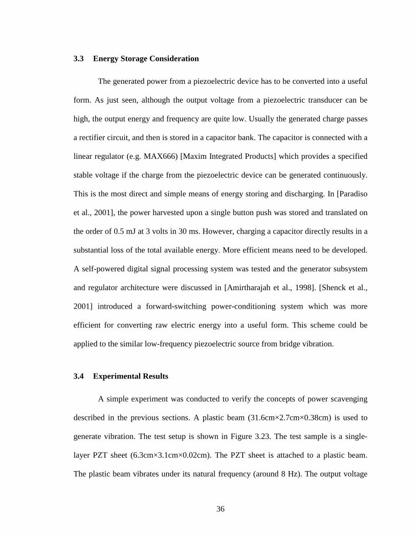
3.3 Energy Storage Consideration
The generated power from a piezoelectric device has to be converted into a useful
form. As just seen, although the output voltage from a piezoelectric transducer can be
high, the output energy and frequency are quite low. Usually the generated charge passes
a rectifier circuit, and then is stored in a capacitor bank. The capacitor is connected with a
linear regulator (e.g. MAX666) [Maxim Integrated Products] which provides a specified
stable voltage if the charge from the piezoelectric device can be generated continuously.
This is the most direct and simple means of energy storing and discharging. In [Paradiso
et al., 2001], the power harvested upon a single button push was stored and translated on
the order of 0.5 mJ at 3 volts in 30 ms. However, charging a capacitor directly results in a
substantial loss of the total available energy. More efficient means need to be developed.
A self-powered digital signal processing system was tested and the generator subsystem
and regulator architecture were discussed in [Amirtharajah et al., 1998]. [Shenck et al.,
2001] introduced a forward-switching power-conditioning system which was more
efficient for converting raw electric energy into a useful form. This scheme could be
applied to the similar low-frequency piezoelectric source from bridge vibration.
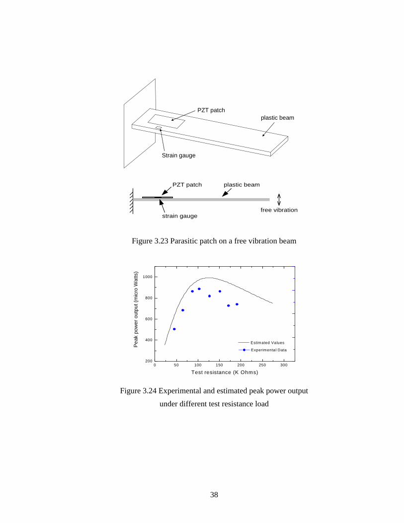
3.4 Experimental Results
A simple experiment was conducted to verify the concepts of power scavenging
described in the previous sections. A plastic beam (31.6cm×2.7cm×0.38cm) is used to
generate vibration. The test setup is shown in Figure 3.23. The test sample is a single-
layer PZT sheet (6.3cm×3.1cm×0.02cm). The PZT sheet is attached to a plastic beam.
The plastic beam vibrates under its natural frequency (around 8 Hz). The output voltage

37
from electrodes on the PZT sheet was observed in an oscillograph. This is a validation
testing for the patch-type generator. The output of PZT sheet subjected to mechanical
vibration is measured, and the strain on the PZT sheet is also obtained from the strain
gauge. The estimated values are calculated based on the strain value by applying the
equations introduced in section 3.2.2. So the experimental results are compared to the
estimated values. Moreover, various load resistances are connected to the patch
generator, and the generated power is compared to the estimated values which are
calculated by equation 3.5.
As shown in Figure 3.23, the single PZT sheet was attached close to the fixed end
of the plastic beam, and a strain gauge was also installed at the same location of the
plastic beam. The free end of the plastic beam was pushed to deflect 4cm then released.
When the free end was pushed down to deflect 4cm, the strain value obtained from the
strain gauge was 103 micro strain. Results show that the output is a periodic signal with
frequency around 8 Hz which is close to the natural frequency of the plastic beam. With
the effect of mechanical damping, the amplitude of the output signal decreased to zero
after 5 seconds. The maximum peak-to-peak open voltage was measured to be around 25
volts. This is close to the estimated open voltage 30 volts, which is calculated based on
the strain value obtained from the strain gauge. The power generation from the patch-type
generator is about 210µW (302µW, estimated value). The peak power output under
various load resistances is shown in Figure 3.24.
The experimental results show good agreement with the estimated values, and the
patch-type generator performed properly as expected, and a remarkable amount of raw
power is obtained from mechanical vibration.
38
Figure 3.23 Parasitic patch on a free vibration beam
Figure 3.24 Experimental and estimated peak power output
under different test resistance load
PZT patch
strain gauge
plastic beam
free vibration
0 50 100 150 200 250 300200
400
600
800
1000
Test resistance (K Ohms)
Pea
k po
wer
out
put (
mic
ro W
atts
)
Estimated Values
Experimental Data
PZT patchplastic beam
Strain gauge

39
3.5 Comparison to other forms of available energy
Solar radiation is an attractive source for energy scavenging as its technology is
well developed. A highway bridge has large amounts of surface exposed to sun light. No
doubt that the solar energy collection transducer can
provide abundant electric power on a sunny day. The
available energy is decreased to roughly one
hundredth of that on a cloudy day, and to one
thousandth for indoor lighting conditions. When
solar cells are placed on bridges, they are not always
exposed directly to the sun even on sunny days. At
locations of interior girders, the illumination is quite
low and it is similar to indoor lighting conditions.
Many types of solar cells have been fabricated and studied. New solar cells have
efficiency as high as 30%. Reference [Lee et al., 1995] introduces a miniaturized high-
voltage solar array (100 cells in 1 cm2) and it was utilized as a power supply for MEMS.
SmartDust [Warneke et al., 2002] was designed to be powered by a SOI solar cell array
which could harvest around 1 mW/mm2 in full sunlight or 1 µW/mm2 under bright indoor
illumination with 10 to 12% efficiency.
Flexible solar panels are now commercially available. Figure 3.25 shows a 5cm
×3.8cm PowerFilm 3V 22mA solar panel supplied by Iowa Thin Film Technologies
[Iowa Thin Film Technologies, Inc]. The power output is around 66 mW for direct sun
(100%) and 0.1mW under low illumination conditions (0.1%). So the power generation
density is in the range of 3.4mW/cm2 to 5µW/cm2.
Figure 3.25 Solar panel

40
Table 3.3 Power generation comparison
The piezoelectric based power generation density is in the range of 0.0004 to
1mW/cm2. This is quite low compared to that of solar cells in sunny conditions. Table 3.3
shows the comparison. Even so, it is hard to say that solar power generation is the best
choice to supply power for sensors in a bridge. The vibration-induced power generation
has its competitive advantages. It is totally independent of climate and weather. At this
point, solar cells are preferred in sunny conditions. Anytime the bridge is in use,
piezoelectric transducers can generate power continuously both in daytime and nighttime.
Moreover vibration-induced power generation is the most feasible means for powering
embedded sensors. So a good idea would be to combine a vibration-based generator and
solar cells together to power sensors in a bridge.
For a wireless sensor system, various operations consume different amount of
power. Usually the operations include sensing/data processing, data transmission and
system sleeping. The operation of sensing/data processing is to acquire the changes (e.g.:
resistance change) of sensors, and process the raw data (e.g.: delete some unwanted or
unimportant data). The operation of data transmission is to send out useful data as radio
frequency signals, and the operation of system sleeping is to maintain the mode of
sleeping, in which the system terminates other operations temporarily and waits for
activation commands. Table 3.4 shows the power requirement for the operations of a
sunny cloudy nighttime
Solar 3~10mW/cm2 0.01~0.1mW/cm2 0
Vibration 0.0004~1mW/cm2 0.0004~1mW/cm2 0.0004~1mW/cm2

41
wireless sensor system. The estimation of power scavenging from both solar and bridge
vibration is based on a 10 cm2 generator and solar cell. In sunny days, the harvested
power is sufficient for the operations of data transmission, sensing and data processing.
In nighttime, the harvested power from bridge vibration is still enough for sensing, data
processing and limited data transmission.
Table 3.4 Power obtained v.s. Power Demand
Power Obtained (based on 10 cm2) Power Demand [Amirtharajah et al, 1998], [Paradiso et al., 2001], [Arms et al., 2003], [Vittoz, 1994]
Daytime (sunny)
Nighttime Sensing/data procesing
Data transmission
System sleeping
Solar 30~100mW N/A
Vibration 0.004~10mW 0.004~10mW
Sloar+Vibration 30~110mW 0.004~10mW
0.1~10mW 5~50mW 0.01~0.1mW

42
Chapter 4
Resonant Beam-type Strain Sensor
Because traditional resistance strain gauges drift significantly over even short
periods of time, they are not suitable for the purpose of “embedding”. A more stable
strain sensor that is easily integrated with transceivers and system circuits is more
desirable. In this chapter, a resonant beam strain sensor using standard CMOS MEMS
technology [The MOSIS Service] is presented. Standard CMOS has been widely used to
fabricate various sensors [Baltes, 1993], [Eyre et al., 1998]. The device in this chapter is
a beam fixed at both ends for which the resonant frequency is determined by its axial
stress. Changes in its axial stress give changes in its resonant frequency. The beams can
be formed from metals or poly-silicon used in standard CMOS processing by etching
thick field oxides away from underneath a beam.
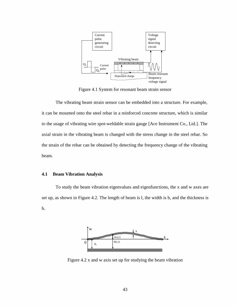
The system of the vibrating beam strain sensor is shown in Figure 4.1. A current
pulse generating circuit creates a positive pulse to charge up the capacitance with large
charge Q1 (to induce the beam vibration) and the discharge of the charge Q2 < Q1 (to
leave a small amount of charge Q for detecting the beam vibration). The reason this
scheme is chosen is explained in Section 4.3. The beam resonant frequency reflects the
axial strain on the beam.
43
Current pulse generating circuit
Current pulse
+ + + + +
- - - - -
Deposited charge
Vibrating beam
Beam resonant frequency voltage signal
Voltage signal detecting circuit
Q1
Q2
Figure 4.1 System for resonant beam strain sensor
The vibrating beam strain sensor can be embedded into a structure. For example,
it can be mounted onto the steel rebar in a reinforced concrete structure, which is similar
to the usage of vibrating wire spot-weldable strain gauge [Ace Instrument Co., Ltd.]. The
axial strain in the vibrating beam is changed with the stress change in the steel rebar. So
the strain of the rebar can be obtained by detecting the frequency change of the vibrating
beam.
4.1 Beam Vibration Analysis
To study the beam vibration eigenvalues and eigenfunctions, the x and w axes are
set up, as shown in Figure 4.2. The length of beam is l, the width is b, and the thickness is
h.
d0
d(x,t)
w(x,t) x
w
0
h
Figure 4.2 x and w axis set up for studying the beam vibration

44
In general, the differential equation of motion for beam structure is given by
equation 4.1 [Sniegowski et al., 1999]:
2 2 2 2
2 2 2 2
( , ) ( , ) ( , )( , )
w x t w x t w x tEI A P q x t
x x t xρ ∂ ∂ ∂ ∂+ − = ∂ ∂ ∂ ∂
(4.1)
where w(x,t) is the vertical deformation function of position x and time t. E is the
Young’s module, I is moment of inertia, ρ is density of the beam, A is the cross sectional
area of the beam. P is the internal axial load applied on the beam and P=εEA, where ε is
axial strain. q(x, t) is the external load on the beam. When there is neither axial nor
perpendicular external load on the beam, the equation of motion can be written as
equation 4.2.
2 2 2
2 2 2
( , ) ( , )0
w x t w x tEI A
x x tρ ∂ ∂ ∂+ = ∂ ∂ ∂
(4.2)
To obtain analytical solutions, separation of variables can be applied as shown in
equation 4.3 [Shames et al., 1991].
( , ) ( ) ( )w x t W x T t= (4.3)
Under the boundary conditions of both ends of the beam being clamped, the
eigenfunctions can be solved as shown in equations 4.4 and 4.5.
( )( ) cosn n nT t W tω α= + (4.4)
( ) ( ) ( ) ( )( ) ( ) ( ) ( )( )cos cosh
( ) cosh cos sin sinhsin sinh
n nn n n n n
n n
k l k lW x k x k x k x k x
k l k l
−= − + ⋅ −− (4.5)
in which ωn and kn are:
( ) ( )cos cosh 1n nk l k l = (4.6)

45
2 4n n
EIk
Aω ρ= n=1,2,3… (4.7)
When an axial force P is applied uniformly on the beam and the perpendicular
external load on the beam is zero, the equation of motion of the beam can be written as
equation 4.8.
2 2 2 2
2 2 2 20
w w wEI A P
x x t xρ ∂ ∂ ∂ ∂+ − = ∂ ∂ ∂ ∂
(4.8)
It is quite difficult to solve equation 4.8 analytically. One way to solve for the
resonant frequency is the Rayleigh-Ritz method, and the solution has the form as shown
in equation 4.9:
( )( , ) ( ) cosw x t W x tω α= + (4.9)
with W(x) as a trial function which satisfies the boundary conditions. Then ( , )w x t can be
solved by this method, and the beam resonant frequency ω is a function of the strain
applied on the beam. In this thesis, finite element code ANSYS is applied to simulate a
vibrating beam under axial forces.
4.2 ANSYS Simulation Result
In this section, the resonant frequency variation with respect to the strain is
presented. First, the situation when there is no pre-tension added on the beam was
studied. Later, a pre-tensioned beam scheme is considered because the strain gauge
should work under tension forces and compression forces. The simulation is done by
using ANSYS [ANSYS, Inc., 1998].

46
4.2.1 Beam with no pre-tension
The schematic diagram of the vibrating MEMS beam is shown in Figure 4.3. The
studied model is an fixed-end beam with length l of 100 micron, width of b=15 micron,
and thickness of h=2 micron. The resonant frequencies of the beam structure under
various situations of longitudinal axial stress are calculated in ANSYS. The composite
material consists of SiO2 and Metal layer (Aluminum). The Young’s Modulus E and
density ρ are given: for SiO2, ρ = 2200 Kg/m3, E=57 to 85 GPa; for Aluminum, ρ = 2702
Kg/m3, E=70 GPa [Gardner et al., 2001])
While applying a tensile stress σ along the beam, the strain in the beam is ε=σ/E.
The resonant frequency change can be observed when the strain in the beam is changed.
The ratio of the loaded resonant frequency and unloaded one, fr/f0, is used to measure the
resonant frequency change with respect to strain change. Figure 4.4 shows that the ratio
fr/f0 has approximately a linear behavior with strain change.
Figure 4.3 Schematic diagram of the vibrating MEMS beam

47
0 500 1000 1500 2000
1.0
1.1
1.2
1.3
1.4
1.5
f r / f 0
Strain (10-6 m/m)
Figure 4.4 MEMS beam resonant frequency response with the strain change.
With zero longitudinal axial stress in the beam, its resonant frequency is 1133.08
KHz. Under an application of 500 micro strains in tension, the resonant frequency is
shifted to 1300.83 KHz. The calculation result shows that the resonant beam is sensitive
to the axial strain change as low as 1 micro strain with an increase of resonant frequency
of about 0.5 KHz for 1 micro strain in tension.
4.2.2 Pre-tensioned MEMS Beam
A strain gauge is used to measure both tensile and compressive strain change in a
structure. For the MEMS resonant beam strain gauge presented here, a small compressive
stress will easily make the thin beam structure buckle. There have been studies and
reported results on growing pre-stressed layers [Ferman, 1999]. MOS fabrication is also
adopting the technology of growing pre-strained layers in MOS transistor fabrication to
improve the performance and to look for new devices [Ernst et al., 2002].The making of
pre-tensioned beams is not well developed, but it is possible.

48
For example, when the beam is pre-tensioned under 1000 micro strains, the initial
resonant frequency f0 will be 1447.33 KHz. If an external compressive force is applied on
the strain gauge, let’s say, 500 micro strains generated in compression, there is still 500
micro strains in tension in the beam. The resonant frequency is shifted to fr =1300.83KHz
comparing to1447.33KHz.
4.3 Capacitance Excitement of the Beam Vibration
To excite the beam vibration, a pulse of current is used to charge the capacitance
plates, with a large charge Q1. Then the Coulumb force on the beam bends the beam and
excites the vibration. The current-pulse driven electrostatic actuators are examined in
[Castañer et al., 2001].
The Coulumb force, q0, per unit length on the bridge is given in equation 4.10:
2
0 20
1
2
l bε= ⋅ (4.10)
Under a uniform force, q0, per unit length perpendicular to the beam, the deformation
equation of the resonant beam is:
( )4
04 4
1
21 cos
8 n
nq l l
w xEI n
π
π∞
=
− = ∑ (4.11)
The mid point of the beam has the maximum deformation:
( )4 40 04 4 4
1
1 cos 41
2 8 162n
nq l q llw
EI n EI
ππ π
∞
=
− = ≅ ∑ (4.12)
To be able to excite the beam, a charge Q1 has to be relatively large so the
Coulumb force could give the beam enough deformation. Assuming the mid point

49
deflection is 0.1 micro meters, the required charge on the beam is about 8.4×10⁻¹³
Coulumbs based on equations 4.10 to 4.12. This is much smaller than the charge
generated from a PZT patch described in section 3.2.2. The generated charge from the
PZT patch is in the order of 10-6:
-8 -60Q=C U=8×10 Farads×32volts=2.6×10 Coulumbs (4.13)
So the harvested power from bridge vibration, as described in section 3, is sufficient to
excite the beam considered here.
Since q(x,t) plays an important role in equation 4.1 which describe the motion of
the beam, solution of the eigenvalues cannot be usually done in closed-form. Also, the
resonant frequency of the beam is also charge dependant, something that leads to
difficulty for calibration.
The scheme considered to solve this problem here is to use a positive current
pulse, followed by a negative pulse. Therefore, the capacitance is charged up with a large
Q1 to excite the beam vibration. Then the capacitance is discharged by a slightly smaller
charge, Q2. Only a small amount of charge, Q1-Q2, is left on the capacitance. Since the
charge is small, the remaining Coulumb force on the beam is negligible in the equation of
motion. Equations 4.2 and 4.8 can be used to describe the motion of the beam without
and with axial force.
4.4 Capacitance Detection of the Beam Resonant Frequency
The beam resonant frequency can be determined by measuring the output AC
voltage frequency. The output voltage is related to the capacitance between the vibrating

50
beam and bottom plate. To calculate the capacitance, as shown in Figure 4.2, first look at
the infinitesimally small capacitance, which is expressed by equation 4.14,
0( , )( , )
bC x t dx
d x t
ε∆ = (4.14)
in which ε0=8.85×10⁻¹² farads/m, the permittivity of vacuum,
and
0( , ) ( , )d x t w x t d= + (4.15)
For 0( , )w x t d<< ,
0 0
0 0 0
0
1 ( , )( , ) 1
( , )1
b b w x tC x t
w x td d dd
ε ε ∆ = ⋅ ≅ ⋅ − +(4.16)
Then the capacitance between the two plates can be expressed as equation 4.17:
0
0 00 0
( , )( ) ( , ) 1
l lb w x tC t C x t dx
d d
ε = ∆ = ⋅ − ∫ ∫ (4.17)
Equation 4.17 can be rewritten as:
00 0
1( ) 1 ( , )
l
C t C w x t dxd l
= − ∫ (4.18)
in which C0 is the capacitance of the beam with no deformation:
00
0
blC
d
ε= (4.19)
where d0 is the gap distance between the vibrating beam and the substrate.
The current pulse generation circuit charges up the capacitance with fixed charge
quantantity Q, then the voltage between the two plates can be expressed as equation 4.19.

51
( )( )
QV t
C t= (4.20)
For 0),( dtxw << , and with 00 / CQV = ,
0
0 0
( )1
1 ( , )l
VV t
w x t dxd l
= − ∫(4.21)
Normally, when the beam is excited to vibrate, many modes exist. When the
uniformly distributed force is added to excite the beam vibration, the dominant mode is
the fundamental mode. To simplify the analysis, only the first mode is considered in this
case. The capacitance and voltage are expressed by equations 4.18 and 4.21.
As shown in equation 4.21, V(t) has the same frequency as w(x,t), so the small
AC voltage signal has the same frequency as the resonant frequency of the beam.
Therefore, by detecting the AC voltage frequency, the strain on the beam can be
obtained.
4.5 Temperature Compensation
Temperature compensation is a significant issue for a strain sensor. The ambient
temperature effect can be compensated by measuring the temperature with a strain-
insensitive resonant beam. The strain-insensitive beam can be a cantilevered beam with
the same width as the strain-sensitive beam, but it is detached from one support so that its
vibration is not affected by the strain, as shown in Figure 4.5.

52
Figure 4.5 Schematic diagram of compensation beam structure
The signal out from the compensation cantilever beam can be compared to its
calibration values so as to obtain the temperature effect. So the signal out from the fix-
end resonant beam can be adjusted.
In this chapter, a scheme of using resonant beam to detecting the strain on the
beam has been demonstrated. The theoretical analysis is given along with the ANSYS
simulation results. Also, a temperature compensation scheme is provided. The results
show that detection of the AC voltage frequency can be used to detect strain.

53
Chapter 5
Measurement of Propagation Attenuation through Concrete
Embedded sensors are designed to be mounted onto steel rebars of a reinforced
concrete structure, and the strain information can be sent out via a radio frequency
transceiver module as described in Chapter 2. In this way, the reliance of wires for
communicating between sensors and central units can be eliminated. Chapter 3 shows
that the harvested power from bridge vibration and solar cells can provide sufficient
power supply for the operations of the embedded sensor system. However, an important
issue has to be considered: signal attenuation in concrete. The higher the attenuation is,
the more power a transceiver module consumes in order to ensure that the received signal
strength can be sustained in a detectable level. The investigation on the signal attenuation
in concrete provides a reference for transceiver design and embedded sensors placement.
In this chapter, a theoretical study is presented and validates experimental
measurements. The measurements are taken at the 900 MHz radio frequency range which
is an unlicensed Industrial, Scientific, Medical (ISM) radio band widely used in civil
applications.
5.1 Electromagnetic Wave Propagation
5.1.1 Reflection and Transmission Coefficient
Consider a uniform plane wave impinging from medium 1 (ε1, µ1) to medium 2
(ε2, µ2). ε, µ are the electric permittivity and magnetic permittivity of the materials. At the

54
boundary of two different materials, part of the incident energy is reflected back into
medium 1 and the rest of the energy is transmitted into medium 2. The normal of the
boundary and the incident wave propagation vector form the plane of incidence, as shown
in Figure 5.1 The angle of incidence is denoted as θ1, and the angle of transmission is
denoted as θ2. θ2 can be obtained from Snell’s law:
1 1 12 1
2 2
sin ( sin )µ εθ θµ ε
−= (5.1)
Air and construction material such as concrete, wood etc. are low conducting
medium, and their relative magnetic permittivity are approximately equal to 1.
1 2 0µ µ µ= = (5.2)
µ0 is the magnetic permittivity of free space and equal to 74 10π −× Henry/meter.
So equation 5.1 can be written as:
1 12 1
2
sin ( sin )εθ θε
−= (5.3)
55
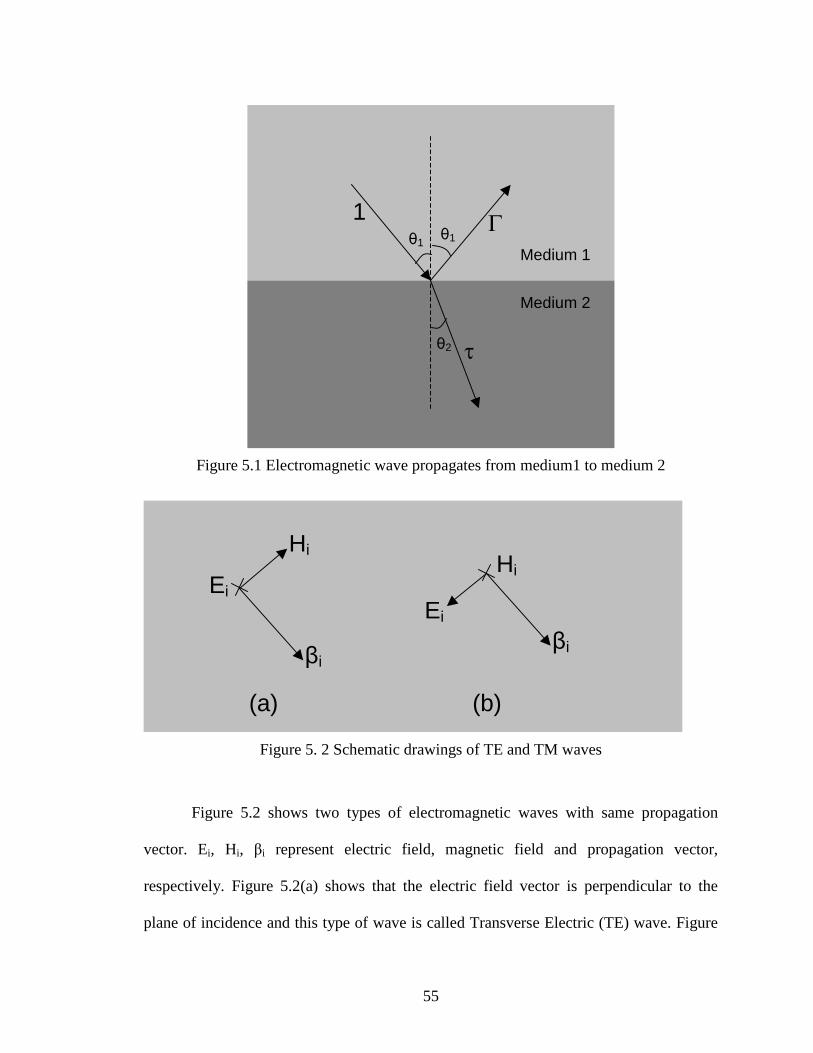
Figure 5.1 Electromagnetic wave propagates from medium1 to medium 2
Figure 5. 2 Schematic drawings of TE and TM waves
Figure 5.2 shows two types of electromagnetic waves with same propagation
vector. Ei, Hi, βi represent electric field, magnetic field and propagation vector,
respectively. Figure 5.2(a) shows that the electric field vector is perpendicular to the
plane of incidence and this type of wave is called Transverse Electric (TE) wave. Figure
Hi
Ei
βi
Hi
Ei
βi
(a) (b)
θ1θ1
θ2
Medium 1
Medium 2
1 Γ
τ

56
5.2(b) shows that the electric field vector is parallel to the plane of incidence and this
type of wave is called Transverse Magnetic (TM) wave.
When a handheld device is designed to communicate with embedded sensor, it is
necessary to know how much energy of the signal is transmitted into concrete and how
much can be received by sensors. So the reflection coefficient and transmission
coefficient are considered.
The reflection coefficient of TE wave is [Rao, 1999]:
1 1 2 2
1 1 2 2
cos cos
cos cosTE
ε θ ε θε θ ε θ
−Γ =+
(5.4)
The transmission coefficient of TE wave is [Rao, 1999]:
1 1
1 1 2 2
2 cos
cos cosTE
ε θτ ε θ ε θ=+
(5.5)
The reflection coefficient of TM wave is [Rao, 1999]:
1 2 2 1
1 21 2 1
cos cos
cos cosTM
ε θ ε θε θ ε θ
−Γ =+
(5.6)
The transmission coefficient of TM wave is [Rao, 1999]:
1 1
1 2 2 1
2 cos
cos cosTM
ε θτ ε θ ε θ=+
(5.7)
When a normal wave impinges to the interface (θ1=0), the reflection and
transmission coefficient can be written:
1 2
1 2
ε εε ε
−Γ =+
(5.8)

57
1
1 2
2 ετ ε ε=+
(5.9)
τ=1 means all wave energy is transmitted from medium 1 to medium 2, and τ=0
means all wave energy is reflected at the interface.
5.1.2 Penetration Depth
Consider a plane wave with electric field of the form:
*( 2 )0
jk j ftE E e ρ π− += (5.10)
where *k is complex wave number in direction ρ , and ρ is position vector. *k has real
part rk and imaginary part ik ( *r ik k jk= − ). The plane wave can be written:
( ( ) 2 ) ( 2 )0 0
r i i rj k jk j ft k jk j ftE E e E e eρ π ρ ρ π− − + − − += = (5.11)
It shows that the magnitude of the wave is changed to 0ikE e ρ− . This attenuation is
due to the wave propagation in dielectric material in direction ρ . Attenuation factor can
be written as:
20log( )ikeγ = (5.12)
The magnitude of the wave can be written in terms of propagation depth pgd :
0i pgk d
magE E e ρ−= (5.13)
For dielectric material with low conductivity, ki can be written in terms of εr’ and
εr” which are the real and imaginary parts of the relative dielectric constant:
0 0( )i rr
k fε µπ εε ′′= ′ (5.14)

58
The relative complex dielectric constant is defined as:
r r rjε ε ε′ ′′= + (5.15)
The real part rε ′ is related to the energy stored in dielectric material and the imaginary
part rε ′′ is related to the energy dissipated.
Penetration depth is defined as the distance at which wave field strength falls to
1/e (36.8%) of its initial value:
0 0
1 rp
i r
dk f
επ ε µ ε
′= = ′′ (5.16)
f is the frequency in Hz of incident wave.
5.2 Dielectric Constant of Concrete
The complex dielectric constant of concrete is dependent on the frequency in low
radio frequencies range, and this dependency is significantly reduced in the microwave
frequencies. This is shown in Figure 5.3. In [Loulizi, 2001], concrete slabs with different
mix constituents were tested to obtain the complex dielectric constant of concrete in the
frequency range of 0.5 to 1.0GHz. Reference [Rhim et al., 1998] also studied the
variation of dielectric constant of concrete with different moisture content in the
frequency range of 0.1 to 20GHz. With the knowledge of dielectric constant, the
transmission coefficient and penetration depth can be obtained from equations 5.4 to 5.7
and 5.16.
Figure 5.3 shows that the complex dielectric constant of concrete is about 9+2j.
Substitute rε ′ =9, rε ′′=2 and f =917.5MHz into equation 5.15, the penetration depth is:

59
6 12 7
915.6
3.14 917.5 10 8.85 10 4 3.14 10 2pd cm− −= =
× × × × × × × ×.
This means that the power of a signal (917.5MHz) falls to 36.8% of its initial value when
it penetrates a depth of 15.6cm in concrete.
Figure 5.3 [Loulizi, 2001] Concrete dielectric constants vs. frequency
5.3 Experimental Set-up and Results
Figure 5.4 shows the experimental set-up. Two antennas are placed facing each
other directly, and the samples are placed between them. Network analyzer is used to take
the measurement of the two antennas. Antennas are connected to the ports of the network
analyzer. The diffraction effects at sample edges have been minimized by increasing
sample area and by making antennas axially perpendicular to sample plane. The S12
reading (in dB) of the network analyzer gives the ratio of the energy received by the
receiving antenna and the energy sent by the transmitting one, S12=20log10(EOUT/EIN).

60
The Two helical antennas are designed with the working range of 0.8 GHz to 1.1
GHz and one functions as the transmitting antenna and the other as the receiving one.
Helical antenna is considered because of its high directivity when it is operating in the
axial mode [Balanis, 1982] as shown in Figure 5.5. Total length L=30cm, diameter
D=10cm, spacing s=7.5cm and total turns N=4. Helical antenna is formed by screwing a
conducting wire. The radiation characteristics of antenna can be changed by controlling
the dimensions. Axial mode is the most practical operation of helical antenna. In this
mode, the majority of radiation intensity is along the helix axis. In order to excite this
mode, the ratio πD/λ must be between 3/4 and 4/3. Usually the helical antenna is used
with a ground plane whose diameter is at least λ/2. For 917MHz wave, λ/2 is equal to
16.4cm. A 20cm×20cm copper plate is used in the experiment.
The nominal impedance of the helical antenna in axial mode is in the range of 100
to 200 Ohms. A thin metal strip is attached to the wire close to the feed point, and the
antenna impedance is then adjusted to 50 Ohms by changing the size of metal strip in
order to match the impedance of transmission lines.

61
Figure 5.4 Schematic drawing of experiment setup
Figure 5.5 Schematic drawing of helical antenna
In order to compare the influence of concrete with other materials, the
measurements were taken under four situations. (a) There is no blocking between the two
SAMPLE
S
L
D
copp
er
plate

62
antennas; (b) Wall board is inserted between the two antennas; (c) Concrete slab with 4.5
inch thickness is inserted between the two antennas. (d) Metal plate is inserted between
the two antennas. The output of the network analyzer gives the S12 reading (in dB) with
respect to wave frequency, as shown in Figure 5.6. X-axis denotes the frequency that
varies from 0.5 to 1.5 GHz. Since the antennas are designed to operate in 0.8 to 1.1 GHz,
Figure 5.6(a) shows that the antenna has less noise in this range. 917.5MHz is marked as
the tracking point and results of measurement taken at this point are presented in Table
5.1.
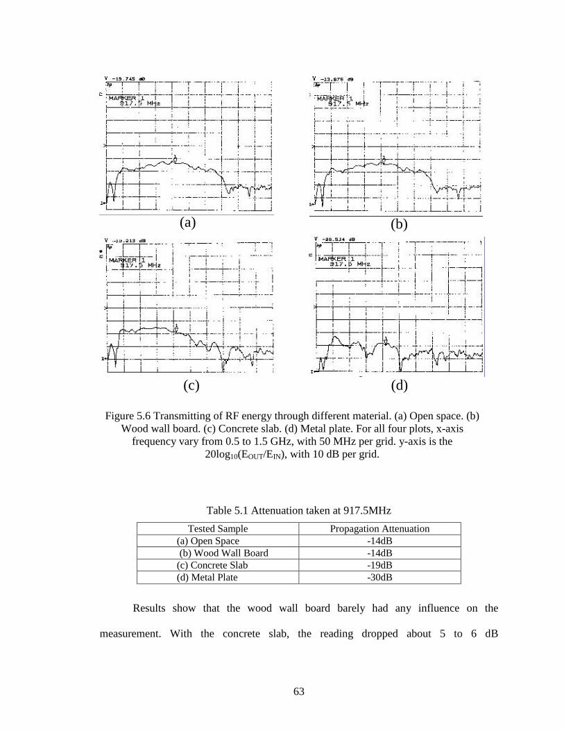
63
(a) (b)
(c) (d)
Figure 5.6 Transmitting of RF energy through different material. (a) Open space. (b) Wood wall board. (c) Concrete slab. (d) Metal plate. For all four plots, x-axis
frequency vary from 0.5 to 1.5 GHz, with 50 MHz per grid. y-axis is the 20log10(EOUT/EIN), with 10 dB per grid.
Table 5.1 Attenuation taken at 917.5MHz
Tested Sample Propagation Attenuation(a) Open Space -14dB(b) Wood Wall Board -14dB
(c) Concrete Slab -19dB(d) Metal Plate -30dB
Results show that the wood wall board barely had any influence on the
measurement. With the concrete slab, the reading dropped about 5 to 6 dB

64
( 21( / 20)/ 10 56.2% 50.1%SOUT INE E to= = ) at 917.5 MHz. That means there is about 50%
power lost. To get an idea about energy level of the scattering field, a metal plate was
inserted between the two antennas to block the direct transmission between them. The
reading dropped about 30 dB ( / 3.2%OUT INE E = ), which is 11 dB more than the loss due
to the concrete slab.
A 5 to 6 dB power loss due to a concrete slab with 4.5 inch (11.4cm) thickness
was found in the experiment. The experimental results also show that the signal
attenuation due to wood wall board is small enough to be neglected. Equation 5.15 shows
that every time the signal (917.5MHz) penetrates a depth of 15.6cm in concrete, the
power of the signal fall to 36.8%. So if the signal penetrates a depth of 4.5 inch (11.4cm),
the power falls to 48.2% ( 0.73e− , from equation 5.13) of its initial value. This is very close
to the experimental results (50.1% to 56.2%).

65
Chapter 6
Summary and Conclusion
In this thesis, an embedded sensor system for structural health monitoring is
described. The sensor system collects structural information by detecting embedded
strain sensors. A power scavenging device is employed to harvest energy from highway
bridge vibration for the power demand of the sensor system. The structural information is
sent back to a handheld monitor wirelessly. This thesis concentrates on three topics:
6.1 power scavenging from highway bridge vibration
Scavenging energy from the ambient is an attractive means to power sensors in
structures. This eliminates the dependence of batteries and allows the sensors to be
tetherless. Power scavenging from traffic-induced vibration of highway bridge vibration
is investigated and PZT (lead zirconate titanate) material is studied as the major
piezoelectric element for power generation. Three mechanisms (Patch, cantilever beam
and stacks) are described that are suitable for sensors to scavenge mechanical energy at
different locations. The PZT patches can also be used to sense the strain changes in
bridge girders. The harvested power is relatively low due to the low strain changes. The
generated power level is about 0.5µW/cm2. Cantilever beam device is design to sense
bridge vibration and generates high strain. The power generation from this mechanism is
about 20µW/cm2 and its dimension can be optimized in order to maximize the generated
power in different vibration environments. PZT stacks and stack arrays have the biggest
potential (1mW/cm2) of the three schemes investigated. By applying the stress

66
amplification scheme, a multilayer stack generates around 1mW power under traffic-
induced vertical compressive stress at the top of girders. A stack array scheme is
designed to be placed in pavement and it makes use of the wheel impact force on
pavement. All calculations are based on the vibration data of a single span girder bridge
using the finite element code ANSYS. The dynamic performance is studied by simulating
trucks moving across the bridge. The results show that the power generation density of
0.0004mW/cm2 (for patches) to 1mW/cm2 (for stacks) can be achieved. Solar power
harvested in solar cells is 3 to 10mW/cm2 in sunny day, and 0.01 to 0.1mW/ cm2 in
cloudy day. Solar cells have the limitation in nighttime and low light conditions.
However the vibration-induced power generation is independent of climate and weather.
So combing vibration-induced power generator and solar cells together is an effective
way to provide power supply for the operation an embedded sensor system, including
sensing, data processing and signal transmission.
6.2 Embedded MEMS beam-type strain sensor
A scheme of using resonant beam to detect the axial strain of the MEMS beam is
demonstrated. The resonant frequency of the vibrating beam is determined by its axial
stress. This allows for detection of under one micro strain (10-6 m/m) change in a 100
micron long beam both for compression and tension. The strain on the beam can be
sampled remotely by observing the resonant frequency of beam while compensation for
such factors as temperature change can be performed. The theoretical analysis is given
along with the ANSYS simulation results and the capacitance excitement and detection

67
technologies are provided. The results show that detection of the AC voltage frequency
provides beam strain information.
6.3 Propagation Attenuation through Concrete at 900 MHz
The propagation of radio frequency signal through concrete at 900 MHz range is
discussed. Measurements are taken to determine the radio frequency energy attenuation
while transmitting through a 4.5 inch concrete slab, a wood wallboard and a metal sheet.
The results show that the wood wallboard has very little effect on signal propagation. A 5
to 6 dB loss due to the concrete slab with 4.5 inch thickness is found. The experimental
results have a good agreement to the theoretical calculations. The theoretical study and
experimental measurement provide a reference for determining embedded depth of
sensors in concrete and designing the transceiver module of an embedded sensor system.
68
References
Ace Instrument Co., Ltd., http://my.ecplaza.net/aceins/3.asp
Amirtharajah R and Chandrakasan A.P., 1998, “Self-Powered Signal Processing Using Vibration-
Based Power Generation,” IEEE Journal of Solid-State Circuits, Vol. 33, No. 5, pp. 687-
695, May
ANSYS, Inc., 1998, Tenth Edition ANSYS Manuals Release 5.5, September
Arms S.W. and Townsend C. P., 2003, “Wireless Strain Measurement Systems
−Applications & Solutions,” Presented at NSF-ESF Joint Conference on
Structural Health Monitoring, Strasbourg, France, October
Balanis C. A., 1982, Antenna Theory Analysis and Design, pp. 386, Harper & Row Publishers
Baltes H. P., 1993, “CMOS as sensor technology,” Sensors and Actuaters, A37-38,
pp.51-56, June-August
Castañer L., Pons J., Nadal-Guardia R. and Rodríguez A., 2001, “Analysis of the
extended operation range of electrostatic actuators by current-pulse drive,”
Sensors and Actuators A 90, pp.181-190
El-hami M., Glynne-Jones P., White N. M., Hill M., Beeby S., James E., Brown A. D., Ross J.
N., 2001, “Design and fabrication of a new vibration-based electromechanical power
generator,” Sensors and Actuators Vol. 92, pp.335-342
Ernst T., Hartmann J.-M., Loup V., Ducroquet F., Dollfus P., Guegan G., Lafond D., Holliger P.,
Toffoli A., and Deleonibus S., 2002, “Fabrication of a Novel Strained SiGe: C-Channel
Planar 55nm nMOSFET for High-Perfomance CMOS,” 2002 Symposium on VLSI
Technol., Hilton Hawaiian Village, Honolulu, HI, June 11-15
Eyre B. and Miller L., 1998, “MEMS Magnetic Sensor in Standard CMOS,” Science
Closure and Enabling Technologies for Constellation Class Missions, edited by V.
Angelopoulos and P. V. Panetta, pp. 99-102, UC Berkeley, Calif.
Ferman M. A. 1999, “Silicon-Based Heterostructures: Strained-Layer Growth by Molecular
Beam Epitaxy,” Cryst. Res. Technol. Vol. 34, pp. 583-595
Friedman D., Heinreich H., and Duan D.W., 1997, “A low-power CMOS integrated circuit for
field-powered radio frequency identification tags,” ISSCC Dig. Tech. Papers, Feb. 1997,
pp. 294-295

69
Gardner J. W., Varadan V. K., Osama A. O., 2001, Microsensors MEMS and Smart Devices.
John Wiley & Sons Ltd, Chichester, England
Glosch H., Ashauer M., Pfeiffer U., Lang W., 1999, “A thermoelectric converter for energy
supply,” Sensors and Actuators Vol. 74, pp.246-250
Glynne-Jones P., Beeby S.P. and White N.M., 2001, “Towards a piezoelectric vibration-powered
microgenerator,” IEE Proc. –Sci. Meas. Technol., Vol. 148, No. 2, pp.68-72, March
Honcharenko W., Bertoni H. L., Dailing J. L., Qian J., and Yee H. D., 1992, “Mechanisms
Governing UHF Propagation on Single Floors in Modern Office Buildings,” IEEE
Transaction on Vehicular Technology, Vol. 41, No. 4, November
Honcharenko W., Bertoni H. L., and Dailing J., 1993, “Mechanism Governing Propagation
Between Different Floors in Buildings,” IEEE Transaction on Antennas and Propagation,
Vol. 41, No. 6, June
Iowa Thin Film Technologies, Inc., http://www.iowathinfilm.com/
Jung K., Bredow J. W., Joshi S. P., 1999, “Electromagnetically coupled embedded sensors,”
Proceedings of SPIE Vol. 3674, Industrial and Commercial Applications of Smart
Structures Technologies
Kendall C. J., 1998, “Parasitic Power Collection in Shoe Mounted Devices,” Thesis of Bachelor
Degree, Massachusetts Institute of Technology, June
Kovács Ádám and Vízváry Zsolt, 2001, “Structural parameter sensitivity analysis of cantilever-
and bridge-type accelerometers,” Sensors and Actuators A 89 (2001) 197-205
Lafortune J. F. and Lecours M., 1990, “Measurement and Modeling of Propagation Losses in a
Building at 900 MHz,” IEEE Transaction on Vehicular Technology, Vol. 39, No. 2, May
Lawton M. C. and McGeehan J. P., 1994, “The Application of a Deterministic Ray Launching
Algorithm for the Prediction of Radio Channel Characteristics in Small-Cell
Environments,” IEEE Transaction on Vehicular Technology, Vol. 43, No. 4, November
Lee J. B., Chen Z., Allen M. G., Rohatgi A. and Arya R., 1995, “A Miniaturized High-Voltage
Solar Cell Array as an Electrostatic MEMS Power Supply,” IEEE Journal of MEMES,
Vol. 4, No. 3, September
Loulizi Amara, 2001, “Development of Ground Penetrating Radar Signal Modeling and
Implementation for Transportation Infrastructure,” Ph.D. Dissertation, Virginia
Polytechnic Institute and State University, February
Lynch J. P., Law K. H., Straser E. G., Kiremidjian A. S. and Kenny T. W., 2000, “The
Development of a Wireless Modular Health Monitoring System for Civil Structures,”

70
Proceedings of the MCEER Mitigation of Earthquake Disaster by Advanced
Technologies (MEDAT-2) Workshop, Las Vegas, NV, USA, November
MathWorks, Inc., http://www.mathworks.com
Maxim Integrated Products, http://www.maxim-ic.com/quick_view2.cfm/qv_pk/1330
Meninger S.,Mur-Miranda J.O., Amirtharajah R, Chandrakasan A.P., Lang J.H., 2001,
"Vibration-to-Electric Energy Conversion," ISPLED99, pp. 48-53
MicroStrain, Inc., http://www.microstrain.com/SG-Link.htm
Morgan Electro Ceramics, http://www.morganelectroceramics.com/
Morgan Electro Ceramics, 2000, “Piezoelectricity High Voltage Generators,” Technical
Publication TP-219
Paradiso J. A. and Feldmeier M, 2001, “A Compact, Wireless, Self-Powered Pushbutton
Controller,” UBICOMP Conference Proceedings, Atlanta GA, Sept. 2001, Springer-
Verlag Berlin Heidelberg,
Pfeifer K. B., Leming S. K., and Rumpf A. N., 2001, “Embedded Self-Powered MicroSensors for
Monitoring the Surety of Critical Buildings and Infrastructures,” Sandia National
Laboratories, SANDIA REPORT, SAND2001-3619, Unlimited Release, Printed
November
Piezo Systems, Inc., Piezo Generator/Sensor Kit Manual, 186 Massachusetts Ave. Cambridge,
MA 02139 USA
Rao Nannapaneni N., 1999, “Elements of Engineering Electromagnetics,” Ftfth Edition,
PRENTICE HALL, Upper Saddle River, NJ 07458
Rhim H. C. and Büyüköztürk R., 1998, “Electromagnetic Properties of Concrete at Microwave
Frequency Range,” ACI Material Journal, pp. 262-271, May-June
Seidel S. Y., and Rappaport T. S., 1994, “Site-Specific Propagation Prediction for Wireless In-
Building Personal Communication System Design,” IEEE Transaction on Vehicular
Technology, Vol. 43, No. 4, November
Sensor Technology Ltd., http://www.sensortech.ca/igniter.html
Shames I. H., and Dym C. L., 1991, Energy and Finite Element Methods in Structural Mechanics.
Taylor & Francis, Levittown, PA
Shearwood C. and Yates R. B., 1997, “Development of an Electromagnetic Microgenerator,”
Electronics Letters, Vol. 33 No. 2, October
71
Shenck N. S. and Paradiso J. A., 2001, “Energy Scavenging With Shoe-Mounted Piezoelectrics,”
IEEE 0272-1732/01
Sniegowski J.J., Guckel H. and Christenson T. R., 1999, “Performance Characteristic of Second
Generation Polysilicon Resonanting Beam Force Transducers,” Solid-State Sensor and
Actuator Workshop, 4th Technical Digest, Hilton Head Island, SC, IEEE, pp. 9-12
Starner T., 1996, “Human powered wearable computing,” IBM Syst. J., Vol. 35, pp. 618-629
Straser E. G., Kiremidjian A S., Law K. H. and Blume J. A., 2000, “A Framework for
Health Monitoring of Structures,” Structures Congress and Exposition, ASCE,
Philadephia, PA, May 8-10
Straser E. G., Kiremidjian A. S., Meng T. H., and Redlefsen L., 1998, “Modular, wireless
network platform for monitoring structures,” Proceedings of the International Modal
Analysis Conference – IMAC, pp. 450-456
The MOSIS Service, http://www.mosis.org/
Vittoz E. A., 1994, “Low-power design: Ways to approach the limits,” ISSCC 1994 Dig.
Tech. Papers, Feb., pp.14-18
Warneke B. A., Scott M. D., Leibowitz B. S., Zhou L., Bellew C. L., Chediak J. A., Kahn J. M.,
Boser B. E., Pister K. S. J., 2002, “An Autonomous 16 mm3 Solar-Powered Node for
Distributed Wireless Sensor Networks,” IEEE 0-7803-7454-1/02
Weinberg M. S., 1999, “Working Equations for Piezoelectric Actuators and Sensors,” IEEE
Journal of MEMS, Vol. 8, No. 4
Williams C.B., Pavic A., Crouch R.S., and Woods R.C., 1997, “Feasibility Study of Vibration-
Electric Generator for Bridge Vibration Sensors,” IMAC-XVI Proceeding
Wu J., Quinn V., Bernstein G. H., 2001, “A simple, wireless powering scheme for MEMS
devices,” Proceedings of SPIE Vol. 4559 (2001), MEMS Components and Applications
for Industry, Automobiles, Aerospace, and Communication
Zhang H., Hayashida T., Takashi Yoshino, Shiro Ito and Yoji Nagasawa, 1999, “A Deterministic
Model for UFH Radio Wave Propagation through Building Windows in Cellular
Environments,” IEICE Transaction on Communication, Vol. E82-B, No. 6 June

72