title stata.com epitab perform breslow–day homogeneity test ... addplot(plot) add other plots to...
TRANSCRIPT
Title stata.com
epitab — Tables for epidemiologists
Description Quick start Menu SyntaxOptions Remarks and examples Stored results Methods and formulasAcknowledgments References Also see
Descriptionir is used with incidence-rate (incidence-density or person-time) data. It calculates point estimates
and confidence intervals for the incidence-rate ratio and difference, along with attributable or preventedfractions for the exposed and total population. iri is the immediate form of ir; see [U] 19 Immediatecommands. Also see [R] poisson and [ST] stcox for related commands.
cs is used with cohort study data with equal follow-up time per subject and sometimes with cross-sectional data. Risk is then the proportion of subjects who become cases. It calculates point estimatesand confidence intervals for the risk difference, risk ratio, and (optionally) the odds ratio, along withattributable or prevented fractions for the exposed and total population. csi is the immediate formof cs; see [U] 19 Immediate commands. Also see [R] logistic for related commands.
cc is used with case–control and cross-sectional data. It calculates point estimates and confidenceintervals for the odds ratio, along with attributable or prevented fractions for the exposed and totalpopulation. cci is the immediate form of cc; see [U] 19 Immediate commands. Also see [R] logisticfor related commands.
tabodds is used with case–control and cross-sectional data. It tabulates the odds of failure againsta categorical explanatory variable expvar. If expvar is specified, tabodds performs an approximateχ2 test of homogeneity of odds and a test for linear trend of the log odds against the numerical codeused for the categories of expvar. Both tests are based on the score statistic and its variance; seeMethods and formulas. When expvar is absent, the overall odds are reported. The variable varcase iscoded 0/1 for individual and simple frequency records and equals the number of cases for binomialfrequency records.
Optionally, tabodds tabulates adjusted or unadjusted odds ratios, using either the lowest levelsof expvar or a user-defined level as the reference group. If adjust(varlist) is specified, it producesodds ratios adjusted for the variables in varlist along with a (score) test for trend.
mhodds is used with case–control and cross-sectional data. It estimates the ratio of the odds offailure for two categories of expvar, controlled for specified confounding variables, varsadjust, andtests whether this odds ratio is equal to one. When expvar has more than two categories but noneare specified with the compare() option, mhodds assumes that expvar is a quantitative variable andcalculates a 1-degree-of-freedom test for trend. It also calculates an approximate estimate of the logodds-ratio for a one-unit increase in expvar. This is a one-step Newton–Raphson approximation tothe maximum likelihood estimate calculated as the ratio of the score statistic, U , to its variance, V(Clayton and Hills 1993, 103).
mcc is used with matched case–control data. It calculates McNemar’s chi-squared; point estimatesand confidence intervals for the difference, ratio, and relative difference of the proportion with thefactor; and the odds ratio and its confidence interval. mcci is the immediate form of mcc; see[U] 19 Immediate commands. Also see [R] clogit and [R] symmetry for related commands.
1

2 epitab — Tables for epidemiologists
Quick startCohort studies
IRR and difference for the number of cases stored in cases for binary indicator exposed given timeexposed time
ir cases exposed time
Crude and Mantel–Haenszel combined IRRs with test of homogeneity for strata defined by svar
ir cases exposed time, by(svar)
As above, and standardize the IRR by weighting variable wvar1
ir cases exposed time, by(svar) standard(wvar1)
As above, but use person-time of the unexposed group as weightsir cases exposed time, by(svar) estandard
IRR and difference for 10 cases over 50 person-years in the exposed group and 15 cases over 100person-years in the unexposed group
iri 10 15 50 100
Risk difference and ratio with binary indicators case and exposed using cumulative incidence datacs case exposed [fweight=wvar2]
Add odds ratios and calculate Fisher’s exact pcs case exposed [fweight=wvar2], or exact
Internally standardized risk ratio for strata defined by svar
cs case exposed [fweight=wvar2], by(svar) istandard
Risk difference and ratio for 12 cases and 55 noncases among exposed subjects and 16 cases and125 noncases among unexposed subjects
csi 12 16 55 125
Case–control studies
Odds ratios from summary data with binary indicators case and exposed and frequency weightwvar3
cc case exposed [fweight=wvar3]
As above, but stratify analysis by svar and perform Breslow–Day and Tarone’s homogeneity testscc case exposed [fweight=wvar3], by(svar) bd tarone
Odds ratios for 37 exposed cases, 148 unexposed cases, 7 exposed controls, and 137 unexposedcontrols
cci 37 148 7 137
Odds of binary event against catvar using summary data with frequency weight wvar4tabodds event catvar [fweight=wvar4]
As above, but report odds ratios with the fourth level of catvar as the referencetabodds event catvar [fweight=wvar4], or base(4)

epitab — Tables for epidemiologists 3
As above, but tabulate Mantel–Haenszel adjusted odds ratios adjusting for values of categoricalvariable a
tabodds event catvar [fweight=wvar4], base(4) adjust(a)
Graph odds and confidence intervals against categories of catvartabodds event catvar [fweight=wvar4], ciplot
Odds ratios for the effect of catvar on event controlling for categorical variable a using summarydata with frequency weight wvar5
mhodds event catvar a [fweight=wvar5]
As above, but calculate odds ratios for each level of svarmhodds event catvar a [fweight=wvar5], by(svar)
Maximum likelihood estimate of odds ratio for a equal to 4 compared with a equal to 1mhodds event a [fweight=wvar5], compare(4,1)
Statistics on the difference in the proportion with the factor for exposed cases indicated in expcaseand exposed controls indicated in expcontrol using summary data with frequency weight wvar6
mcc expcase expcontrol [fweight=wvar6]
As above, but indicate that there are 4 pairs where both cases and controls were exposed, 9 pairswhere the case was exposed but the control was not, 3 pairs where the control was exposed butthe case was not, and 14 pairs where neither subject was exposed
mcci 4 9 3 14

4 epitab — Tables for epidemiologists
Menuir
Statistics > Epidemiology and related > Tables for epidemiologists > Incidence-rate ratio
iri
Statistics > Epidemiology and related > Tables for epidemiologists > Incidence-rate ratio calculator
cs
Statistics > Epidemiology and related > Tables for epidemiologists > Cohort study risk-ratio etc.
csi
Statistics > Epidemiology and related > Tables for epidemiologists > Cohort study risk-ratio etc. calculator
cc
Statistics > Epidemiology and related > Tables for epidemiologists > Case-control odds ratio
cci
Statistics > Epidemiology and related > Tables for epidemiologists > Case-control odds-ratio calculator
tabodds
Statistics > Epidemiology and related > Tables for epidemiologists > Tabulate odds of failure by category
mhodds
Statistics > Epidemiology and related > Tables for epidemiologists > Ratio of odds of failure for two categories
mcc
Statistics > Epidemiology and related > Tables for epidemiologists > Matched case-control studies
mcci
Statistics > Epidemiology and related > Tables for epidemiologists > Matched case-control calculator

epitab — Tables for epidemiologists 5
Syntax
Cohort studies
ir varcase varexposed vartime
[if] [
in] [
weight] [
, ir options]
iri #a #b #N1 #N2
[, level(#)
]cs varcase varexposed
[if] [
in] [
weight] [
, cs options]
csi #a #b #c #d[, csi options
]
Case–control studies
cc varcase varexposed[
if] [
in] [
weight] [
, cc options]
cci #a #b #c #d[, cci options
]tabodds varcase
[expvar
] [if] [
in] [
weight] [
, tabodds options]
mhodds varcase expvar[
varsadjust] [
if] [
in] [
weight] [
, mhodds options]
Matched case–control studies
mcc varexposed case varexposed control
[if] [
in] [
weight] [
, level(#)]
mcci #a #b #c #d[, level(#)
]ir options Description
Options
by(varname[, missing
]) stratify on varname
estandard combine external weights with within-stratum statisticsistandard combine internal weights with within-stratum statisticsstandard(varname) combine user-specified weights with within-stratum statisticspool display pooled estimatenocrude do not display crude estimatenohom do not display homogeneity testird calculate standard incidence-rate differencelevel(#) set confidence level; default is level(95)

6 epitab — Tables for epidemiologists
cs options Description
Options
by(varlist[, missing
]) stratify on varlist
estandard combine external weights with within-stratum statisticsistandard combine internal weights with within-stratum statisticsstandard(varname) combine user-specified weights with within-stratum statisticspool display pooled estimatenocrude do not display crude estimatenohom do not display homogeneity testrd calculate standardized risk differencebinomial(varname) number of subjects variableor report odds ratiowoolf use Woolf approximation to calculate SE and CI of the odds ratioexact calculate Fisher’s exact plevel(#) set confidence level; default is level(95)
csi options Description
or report odds ratiowoolf use Woolf approximation to calculate SE and CI of the odds ratioexact calculate Fisher’s exact plevel(#) set confidence level; default is level(95)
cc options Description
Options
by(varname[, missing
]) stratify on varname
estandard combine external weights with within-stratum statisticsistandard combine internal weights with within-stratum statisticsstandard(varname) combine user-specified weights with within-stratum statisticspool display pooled estimatenocrude do not display crude estimatenohom do not display homogeneity testbd perform Breslow–Day homogeneity testtarone perform Tarone’s homogeneity testbinomial(varname) number of subjects variablecornfield use Cornfield approximation to calculate CI of the odds ratiowoolf use Woolf approximation to calculate SE and CI of the odds ratioexact calculate Fisher’s exact plevel(#) set confidence level; default is level(95)
epitab — Tables for epidemiologists 7
cci options Description
cornfield use Cornfield approximation to calculate CI of the odds ratiowoolf use Woolf approximation to calculate SE and CI of the odds ratioexact calculate Fisher’s exact plevel(#) set confidence level; default is level(95)
tabodds options Description
Main
binomial(varname) number of subjects variablelevel(#) set confidence level; default is level(95)
or report odds ratioadjust(varlist) report odds ratios adjusted for the variables in varlistbase(#) reference group of control variable for odds ratiocornfield use Cornfield approximation to calculate CI of the odds ratiowoolf use Woolf approximation to calculate SE and CI of the odds ratiograph graph odds against categoriesciplot same as graph option, except include confidence intervals
CI plot
ciopts(rcap options) affect rendition of the confidence bands
Plot
marker options change look of markers (color, size, etc.)marker label options add marker labels; change look or positioncline options affect rendition of the plotted points
Add plots
addplot(plot) add other plots to the generated graph
Y axis, X axis, Titles, Legend, Overall
twoway options any options other than by() documented in [G-3] twoway options
mhodds options Description
Options
by(varlist[, missing
]) stratify on varlist
binomial(varname) number of subjects variablecompare(v1,v2) override categories of the control variablelevel(#) set confidence level; default is level(95)
fweights are allowed; see [U] 11.1.6 weight.
8 epitab — Tables for epidemiologists
Options
Options are listed in the order that they appear in the syntax tables above. The commands forwhich the option is valid are indicated in parentheses immediately after the option name.
� � �Options (ir, cs, cc, and mhodds) / Main (tabodds) �
by(varname[, missing
]) (ir, cs, cc, and mhodds) specifies that the tables be stratified on
varname. Missing categories in varname are omitted from the stratified analysis, unless optionmissing is specified within by(). Within-stratum statistics are shown and then combined withMantel–Haenszel weights. If estandard, istandard, or standard() is also specified (seebelow), the weights specified are used in place of Mantel–Haenszel weights.
estandard, istandard, and standard(varname) (ir, cs, and cc) request that within-stratumstatistics be combined with external, internal, or user-specified weights to produce a standardizedestimate. These options are mutually exclusive and can be used only when by() is also specified.(When by() is specified without one of these options, Mantel–Haenszel weights are used.)
estandard external weights are the person-time for the unexposed (ir), the total number ofunexposed (cs), or the number of unexposed controls (cc).
istandard internal weights are the person-time for the exposed (ir), the total number of exposed(cs), or the number of exposed controls (cc). istandard can be used to produce, among otherthings, standardized mortality ratios (SMRs).
standard(varname) allows user-specified weights. varname must contain a constant within stratumand be nonnegative. The scale of varname is irrelevant.
pool (ir, cs, and cc) specifies that, in a stratified analysis, the directly pooled estimate alsobe displayed. The pooled estimate is a weighted average of the stratum-specific estimates usinginverse-variance weights, which are the inverse of the variance of the stratum-specific estimate.pool is relevant only if by() is also specified.
nocrude (ir, cs, and cc) specifies that in a stratified analysis the crude estimate—an estimateobtained without regard to strata—not be displayed. nocrude is relevant only if by() is alsospecified.
nohom (ir, cs, and cc) specifies that a χ2 test of homogeneity not be included in the output ofa stratified analysis. This tests whether the exposure effect is the same across strata and can beperformed for any pooled estimate—directly pooled or Mantel–Haenszel. nohom is relevant onlyif by() is also specified.
ird (ir) may be used only with estandard, istandard, or standard(). It requests that ircalculate the standardized incidence-rate difference rather than the default incidence-rate ratio.
rd (cs) may be used only with estandard, istandard, or standard(). It requests that cs calculatethe standardized risk difference rather than the default risk ratio.
bd (cc) specifies that Breslow and Day’s χ2 test of homogeneity be included in the output of astratified analysis. This tests whether the exposure effect is the same across strata. bd is relevantonly if by() is also specified.
tarone (cc) specifies that Tarone’s χ2 test of homogeneity, which is a correction to the Breslow–Daytest, be included in the output of a stratified analysis. This tests whether the exposure effect is thesame across strata. tarone is relevant only if by() is also specified.

epitab — Tables for epidemiologists 9
binomial(varname) (cs, cc, tabodds, and mhodds) supplies the number of subjects (cases pluscontrols) for binomial frequency records. For individual and simple frequency records, this optionis not used.
or (cs, csi, and tabodds), for cs and csi, reports the calculation of the odds ratio in addition tothe risk ratio if by() is not specified. With by(), or specifies that a Mantel–Haenszel estimateof the combined odds ratio be made rather than the Mantel–Haenszel estimate of the risk ratio.In either case, this is the same calculation that would be made by cc and cci. Typically, cc, cci,or tabodds is preferred for calculating odds ratios. For tabodds, or specifies that odds ratios beproduced; see base() for details about selecting a reference category. By default, tabodds willcalculate odds.
adjust(varlist) (tabodds) specifies that odds ratios adjusted for the variables in varlist be calculated.
base(#) (tabodds) specifies that the #th category of expvar be used as the reference group forcalculating odds ratios. If base() is not specified, the first category, corresponding to the minimumvalue of expvar, is used as the reference group.
cornfield (cc, cci, and tabodds) requests that the Cornfield (1956) approximation be used tocalculate the confidence interval of the odds ratio. By default, cc and cci report an exact intervaland tabodds reports a standard-error–based interval, with the standard error coming from thesquare root of the variance of the score statistic.
woolf (cs, csi, cc, cci, and tabodds) requests that the Woolf (1955) approximation, also knownas the Taylor expansion, be used for calculating the standard error and confidence interval for theodds ratio. By default, cs and csi with the or option report the Cornfield (1956) interval; ccand cci report an exact interval; and tabodds reports a standard-error–based interval, with thestandard error coming from the square root of the variance of the score statistic.
exact (cs, csi, cc, and cci) requests that Fisher’s exact p be calculated rather than the χ2 andits significance level. We recommend specifying exact whenever samples are small. When theleast-frequent cell contains 1,000 cases or more, there will be no appreciable difference betweenthe exact significance level and the significance level based on the χ2, but the exact significancelevel will take considerably longer to calculate. exact does not affect whether exact confidenceintervals are calculated. Commands always calculate exact confidence intervals where they can,unless cornfield or woolf is specified.
compare(v1,v2) (mhodds) indicates the categories of expvar to be compared; v1 defines the numeratorand v2, the denominator. When compare() is not specified and there are only two categories, thesecond is compared to the first; when there are more than two categories, an approximate estimateof the odds ratio for a unit increase in expvar, controlled for specified confounding variables, isgiven.
level(#) (ir, iri, cs, csi, cc, cci, tabodds, mhodds, mcc, and mcci) specifies the confidencelevel, as a percentage, for confidence intervals. The default is level(95) or as set by set level;see [R] level.

10 epitab — Tables for epidemiologists
The following options are for use only with tabodds.
� � �Main �
graph (tabodds) produces a graph of the odds against the numerical code used for the categoriesof expvar. All graph options except connect() are allowed. This option is not allowed with theor option or the adjust() option.
ciplot (tabodds) produces the same plot as the graph option, except that it also includes theconfidence intervals. This option may not be used with either the or option or the adjust()option.
� � �CI plot �
ciopts(rcap options) (tabodds) is allowed only with the ciplot option. It affects the renditionof the confidence bands; see [G-3] rcap options.
� � �Plot �
marker options (tabodds) affect the rendition of markers drawn at the plotted points, including theirshape, size, color, and outline; see [G-3] marker options.
marker label options (tabodds) specify if and how the markers are to be labeled; see[G-3] marker label options.
cline options (tabodds) affect whether lines connect the plotted points and the rendition of thoselines; see [G-3] cline options.
� � �Add plots �
addplot(plot) (tabodds) provides a way to add other plots to the generated graph; see[G-3] addplot option.
� � �Y axis, X axis, Titles, Legend, Overall �
twoway options (tabodds) are any of the options documented in [G-3] twoway options, excludingby(). These include options for titling the graph (see [G-3] title options) and options for savingthe graph to disk (see [G-3] saving option).
Remarks and examples stata.com
Remarks are presented under the following headings:
Incidence-rate dataStratified incidence-rate dataStandardized estimates with stratified incidence-rate dataCumulative incidence dataStratified cumulative incidence dataStandardized estimates with stratified cumulative incidence dataCase–control dataStratified case–control dataCase–control data with multiple levels of exposureCase–control data with confounders and possibly multiple levels of exposureStandardized estimates with stratified case–control dataMatched case–control dataVideo examplesGlossary

epitab — Tables for epidemiologists 11
To calculate appropriate statistics and suppress inappropriate statistics, the ir, cs, cc, tabodds,mhodds, and mcc commands, along with their immediate counterparts, are organized in the wayepidemiologists conceptualize data. ir processes incidence-rate data from prospective studies; cs,cohort study data with equal follow-up time (cumulative incidence); cc, tabodds, and mhodds,case–control or cross-sectional (prevalence) data; and mcc, matched case–control data. With theexception of mcc, these commands work with both simple and stratified tables.
Epidemiological data are often summarized in a contingency table from which various statistics arecalculated. The rows of the table reflect cases and noncases or cases and person-time, and the columnsreflect exposure to a risk factor. To an epidemiologist, cases and noncases refer to the outcomes ofthe process being studied. For instance, a case might be a person with cancer and a noncase mightbe a person without cancer.
A factor is something that might affect the chances of being ultimately designated a case or anoncase. Thus a case might be a cancer patient and the factor, smoking behavior. A person is said tobe exposed or unexposed to the factor. Exposure can be classified as a dichotomy, smokes or doesnot smoke, or as multiple levels, such as number of cigarettes smoked per week.
For an introduction to epidemiological methods, see Walker (1991). For an intermediate treatment,see Clayton and Hills (1993) and Lilienfeld and Stolley (1994). For other advanced discussions, seeKleinbaum, Kupper, and Morgenstern (1982) and Rothman, Greenland, and Lash (2008). For ananthology of writings on epidemiology since World War II, see Greenland (1987). See Jewell (2004)for a text aimed at graduate students in the medical professions that uses Stata for much of the analysis.See Dohoo, Martin, and Stryhn (2010) for a graduate-level text on the principles and methods ofveterinary epidemiologic research; Stata datasets and do-files are available. Also see Dohoo, Martin,and Stryhn (2012) for a text that is a revision of their veterinary epidemiology text, but examplesfrom human epidemiology are used.
Incidence-rate data
In incidence-rate data from a prospective study, you observe the transformation of noncases intocases. Starting with a group of noncase subjects, you monitor them to determine whether they becomecases (for example, stricken with cancer). You monitor two populations: those exposed and thoseunexposed to the factor (for example, multiple X-rays). A summary of the data is
Exposed Unexposed Total
Cases a b a+ bPerson-time N1 N0 N1 +N0
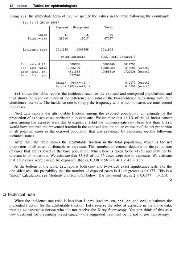
Example 1: iri
It will be easiest to understand these commands if we start with the immediate forms. Remember,in the immediate form, we specify the data on the command line rather than specifying names ofvariables containing the data; see [U] 19 Immediate commands. We have data (Boice and Monson[1977]; reported in Rothman, Greenland, and Lash [2008, 244]) on breast cancer cases and person-years of observation for women with tuberculosis repeatedly exposed to multiple X-ray fluoroscopies,and those not so exposed:
X-ray fluoroscopyExposed Unexposed
Breast cancer cases 41 15Person-years 28,010 19,017
12 epitab — Tables for epidemiologists
Using iri, the immediate form of ir, we specify the values in the table following the command:
. iri 41 15 28010 19017
Exposed Unexposed Total
Cases 41 15 56Person-time 28010 19017 47027
Incidence rate .0014638 .0007888 .0011908
Point estimate [95% Conf. Interval]
Inc. rate diff. .000675 .0000749 .0012751Inc. rate ratio 1.855759 1.005684 3.6093 (exact)Attr. frac. ex. .4611368 .0056519 .722938 (exact)Attr. frac. pop .337618
(midp) Pr(k>=41) = 0.0177 (exact)(midp) 2*Pr(k>=41) = 0.0355 (exact)
iri shows the table, reports the incidence rates for the exposed and unexposed populations, andthen shows the point estimates of the difference and ratio of the two incidence rates along with theirconfidence intervals. The incidence rate is simply the frequency with which noncases are transformedinto cases.
Next iri reports the attributable fraction among the exposed population, an estimate of theproportion of exposed cases attributable to exposure. We estimate that 46.1% of the 41 breast cancercases among the exposed were due to exposure. (Had the incidence-rate ratio been less than 1, iriwould have reported the prevented fraction in the exposed population, an estimate of the net proportionof all potential cases in the exposed population that was prevented by exposure; see the followingtechnical note.)
After that, the table shows the attributable fraction in the total population, which is the netproportion of all cases attributable to exposure. This number, of course, depends on the proportionof cases that are exposed in the base population, which here is taken to be 41/56 and may not berelevant in all situations. We estimate that 33.8% of the 56 cases were due to exposure. We estimatethat 18.9 cases were caused by exposure; that is, 0.338× 56 = 0.461× 41 = 18.9.
At the bottom of the table, iri reports both one- and two-sided exact significance tests. For theone-sided test, the probability that the number of exposed cases is 41 or greater is 0.0177. This is a“midp” calculation; see Methods and formulas below. The two-sided test is 2× 0.0177 = 0.0354.
Technical noteWhen the incidence-rate ratio is less than 1, iri (and ir, cs, csi, cc, and cci) substitutes the
prevented fraction for the attributable fraction. Let’s reverse the roles of exposure in the above data,treating as exposed a person who did not receive the X-ray fluoroscopy. You can think of this as anew treatment for preventing breast cancer—the suggested treatment being not to use fluoroscopy.

epitab — Tables for epidemiologists 13
. iri 15 41 19017 28010
Exposed Unexposed Total
Cases 15 41 56Person-time 19017 28010 47027
Incidence rate .0007888 .0014638 .0011908
Point estimate [95% Conf. Interval]
Inc. rate diff. -.000675 -.0012751 -.0000749Inc. rate ratio .5388632 .277062 .9943481 (exact)Prev. frac. ex. .4611368 .0056519 .722938 (exact)Prev. frac. pop .1864767
(midp) Pr(k<=15) = 0.0177 (exact)(midp) 2*Pr(k<=15) = 0.0355 (exact)
The prevented fraction among the exposed is the net proportion of all potential cases in the exposedpopulation that were prevented by exposure. We estimate that 46.1% of potential cases among thewomen receiving the new “treatment” were prevented by the treatment. (Previously, we estimated thatthe same percentage of actual cases among women receiving the X-rays was caused by the X-rays.)
The prevented fraction for the population, which is the net proportion of all potential cases inthe total population that was prevented by exposure, as with the attributable fraction, depends on theproportion of cases that are exposed in the base population—here taken as 15/56—so it may not berelevant in all situations. We estimate that 18.6% of the potential cases were prevented by exposure.
See Greenland and Robins (1988) for a discussion of how to interpret attributable and preventedfractions.
Example 2: ir
ir works like iri, except that it obtains the entries in the tables by summing data. You specifythree variables: the first represents the number of cases represented by this observation, the secondindicates whether the observation is for subjects exposed to the factor, and the third records the totaltime the subjects in this observation were observed. An observation may reflect one subject or agroup of subjects.
For instance, here is a 2-observation dataset for the table in the previous example:
. use http://www.stata-press.com/data/r15/irxmpl
. list
cases exposed time
1. 41 0 280102. 15 1 19017
If we typed ir cases exposed time, we would obtain the same output that we obtained above.Another way the data might be recorded is
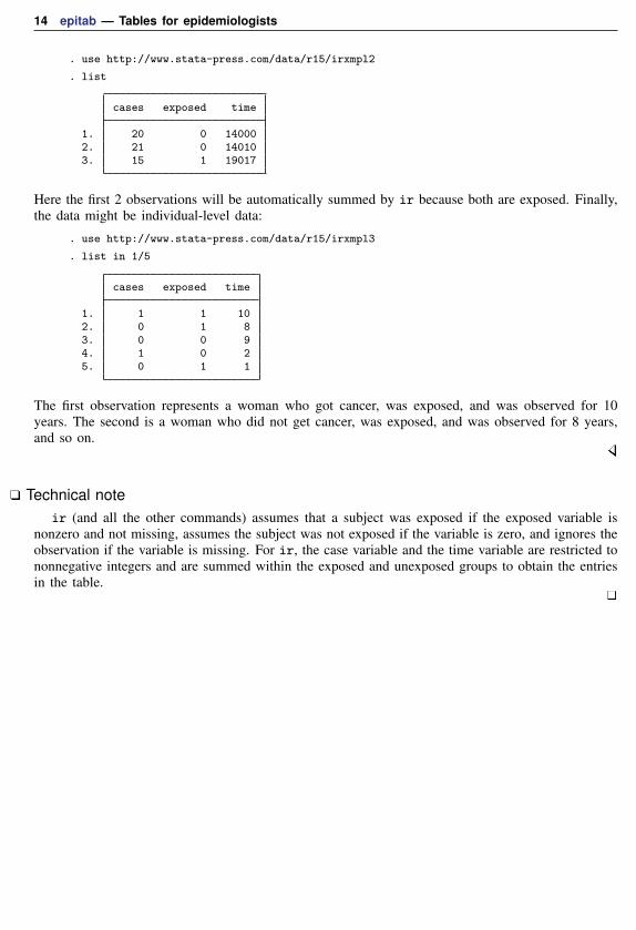
14 epitab — Tables for epidemiologists
. use http://www.stata-press.com/data/r15/irxmpl2
. list
cases exposed time
1. 20 0 140002. 21 0 140103. 15 1 19017
Here the first 2 observations will be automatically summed by ir because both are exposed. Finally,the data might be individual-level data:
. use http://www.stata-press.com/data/r15/irxmpl3
. list in 1/5
cases exposed time
1. 1 1 102. 0 1 83. 0 0 94. 1 0 25. 0 1 1
The first observation represents a woman who got cancer, was exposed, and was observed for 10years. The second is a woman who did not get cancer, was exposed, and was observed for 8 years,and so on.
Technical noteir (and all the other commands) assumes that a subject was exposed if the exposed variable is
nonzero and not missing, assumes the subject was not exposed if the variable is zero, and ignores theobservation if the variable is missing. For ir, the case variable and the time variable are restricted tononnegative integers and are summed within the exposed and unexposed groups to obtain the entriesin the table.
epitab — Tables for epidemiologists 15
Stratified incidence-rate data
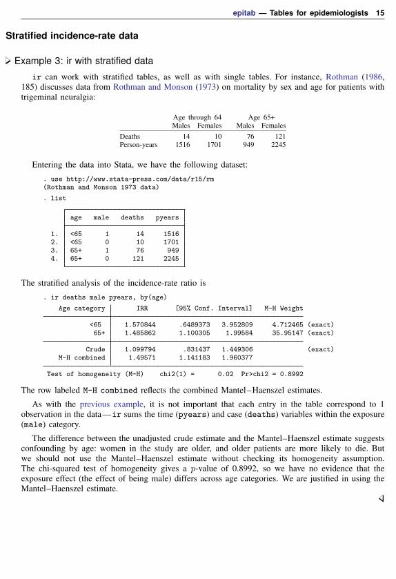
Example 3: ir with stratified data
ir can work with stratified tables, as well as with single tables. For instance, Rothman (1986,185) discusses data from Rothman and Monson (1973) on mortality by sex and age for patients withtrigeminal neuralgia:
Age through 64 Age 65+Males Females Males Females
Deaths 14 10 76 121Person-years 1516 1701 949 2245
Entering the data into Stata, we have the following dataset:
. use http://www.stata-press.com/data/r15/rm(Rothman and Monson 1973 data)
. list
age male deaths pyears
1. <65 1 14 15162. <65 0 10 17013. 65+ 1 76 9494. 65+ 0 121 2245
The stratified analysis of the incidence-rate ratio is
. ir deaths male pyears, by(age)
Age category IRR [95% Conf. Interval] M-H Weight
<65 1.570844 .6489373 3.952809 4.712465 (exact)65+ 1.485862 1.100305 1.99584 35.95147 (exact)
Crude 1.099794 .831437 1.449306 (exact)M-H combined 1.49571 1.141183 1.960377
Test of homogeneity (M-H) chi2(1) = 0.02 Pr>chi2 = 0.8992
The row labeled M-H combined reflects the combined Mantel–Haenszel estimates.
As with the previous example, it is not important that each entry in the table correspond to 1observation in the data—ir sums the time (pyears) and case (deaths) variables within the exposure(male) category.
The difference between the unadjusted crude estimate and the Mantel–Haenszel estimate suggestsconfounding by age: women in the study are older, and older patients are more likely to die. Butwe should not use the Mantel–Haenszel estimate without checking its homogeneity assumption.The chi-squared test of homogeneity gives a p-value of 0.8992, so we have no evidence that theexposure effect (the effect of being male) differs across age categories. We are justified in using theMantel–Haenszel estimate.
16 epitab — Tables for epidemiologists
Technical noteStratification is one way to deal with confounding; that is, perhaps sex affects the incidence of
trigeminal neuralgia and so does age, so the table was stratified by age in an attempt to uncoverthe sex effect. (We are concerned that age may confound the true association between sex and theincidence of trigeminal neuralgia because the age distributions are so different for males and females.If age affects incidence, the difference in the age distributions would induce different incidences formales and females and thus confound the true effect of sex.)
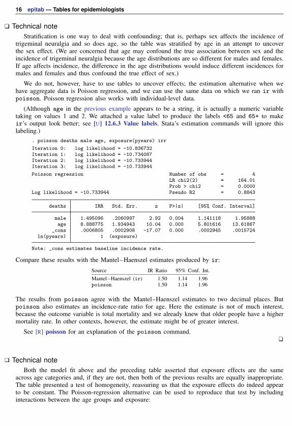
We do not, however, have to use tables to uncover effects; the estimation alternative when wehave aggregate data is Poisson regression, and we can use the same data on which we ran ir withpoisson. Poisson regression also works with individual-level data.
(Although age in the previous example appears to be a string, it is actually a numeric variabletaking on values 1 and 2. We attached a value label to produce the labels <65 and 65+ to makeir’s output look better; see [U] 12.6.3 Value labels. Stata’s estimation commands will ignore thislabeling.)
. poisson deaths male age, exposure(pyears) irr
Iteration 0: log likelihood = -10.836732Iteration 1: log likelihood = -10.734087Iteration 2: log likelihood = -10.733944Iteration 3: log likelihood = -10.733944
Poisson regression Number of obs = 4LR chi2(2) = 164.01Prob > chi2 = 0.0000
Log likelihood = -10.733944 Pseudo R2 = 0.8843
deaths IRR Std. Err. z P>|z| [95% Conf. Interval]
male 1.495096 .2060997 2.92 0.004 1.141118 1.95888age 8.888775 1.934943 10.04 0.000 5.801616 13.61867
_cons .0006805 .0002908 -17.07 0.000 .0002945 .0015724ln(pyears) 1 (exposure)
Note: _cons estimates baseline incidence rate.
Compare these results with the Mantel–Haenszel estimates produced by ir:
Source IR Ratio 95% Conf. Int.Mantel–Haenszel (ir) 1.50 1.14 1.96poisson 1.50 1.14 1.96
The results from poisson agree with the Mantel–Haenszel estimates to two decimal places. Butpoisson also estimates an incidence-rate ratio for age. Here the estimate is not of much interest,because the outcome variable is total mortality and we already knew that older people have a highermortality rate. In other contexts, however, the estimate might be of greater interest.
See [R] poisson for an explanation of the poisson command.
Technical noteBoth the model fit above and the preceding table asserted that exposure effects are the same
across age categories and, if they are not, then both of the previous results are equally inappropriate.The table presented a test of homogeneity, reassuring us that the exposure effects do indeed appearto be constant. The Poisson-regression alternative can be used to reproduce that test by includinginteractions between the age groups and exposure:

epitab — Tables for epidemiologists 17
. poisson deaths male age male#c.age, exposure(pyears) irr
Iteration 0: log likelihood = -10.898799Iteration 1: log likelihood = -10.726225Iteration 2: log likelihood = -10.725904Iteration 3: log likelihood = -10.725904
Poisson regression Number of obs = 4LR chi2(3) = 164.03Prob > chi2 = 0.0000
Log likelihood = -10.725904 Pseudo R2 = 0.8843
deaths IRR Std. Err. z P>|z| [95% Conf. Interval]
male 1.660688 1.396496 0.60 0.546 .3195218 8.631283age 9.167973 3.01659 6.73 0.000 4.810583 17.47226
male#c.age1 .9459 .41539 -0.13 0.899 .3999832 2.236911
_cons .0006412 .0004097 -11.51 0.000 .0001833 .0022434ln(pyears) 1 (exposure)
Note: _cons estimates baseline incidence rate.
The significance level of the male#c.age effect is 0.899, the same as previously reported by ir.
Here forming the male-times-age interaction was easy because there were only two age groups.Had there been more groups, the test would have been slightly more difficult—see the followingtechnical note.
Technical noteA word of caution is in order when applying poisson (or any estimation technique) to more than
two age categories. Say that in our data, we had three age categories, which we will call categories0, 1, and 2, and that they are stored in the variable agecat. We might think of the categories ascorresponding to age less than 35, 35–64, and 65 and above.
With such data, we might type ir deaths male pyears, by(agecat), but we would not typepoisson deaths male agecat, exposure(pyears) to obtain the equivalent Poisson-regressionestimated results. Such a model might be reasonable, but it is not equivalent because we would beconstraining the age effect in category 2 to be (multiplicatively) twice the effect in category 1.
To poisson (and all of Stata’s estimation commands other than anova), agecat is simply onevariable, and only one estimated coefficient is associated with it. Thus the model is
Poisson index = P = β0 + β1male+ β2agecat
The expected number of deaths is then eP , and the incidence-rate ratio associated with a variable iseβ ; see [R] poisson. Thus the value of the Poisson index when male==0 and agecat==1 is β0 +β2,and the possibilities are
male==0 male==1
agecat==0 β0 β0 + β1agecat==1 β0 + β2 β0 + β2 + β1agecat==2 β0 + 2β2 β0 + 2β2 + β1

18 epitab — Tables for epidemiologists
The age effect for agecat==2 is constrained to be twice the age effect for agecat==1—theonly difference between lines 3 and 2 of the table is that β2 is replaced with 2β2. Under certaincircumstances, such a constraint might be reasonable, but it does not correspond to the assumptionsmade in generating the Mantel–Haenszel combined results.
To obtain results equivalent to the Mantel–Haenszel result, we must estimate a separate effect foreach age group, meaning that we must replace 2β2, the constrained effect, with β3, a new coefficientthat is free to take on any value. We can achieve this by creating two new variables and using themin place of agecat. agecat1 will take on the value 1 when agecat is 1 and 0 otherwise; agecat2will take on the value 1 when agecat is 2 and 0 otherwise:
. generate agecat1 = (agecat==1)
. generate agecat2 = (agecat==2)
. poisson deaths male agecat1 agecat2 [freq=pop], exposure(pyears) irr
In Stata, we do not have to generate these variables for ourselves. We could use factor variables:. poisson deaths male i.agecat [freq=pop], exposure(pyears) irr
See [U] 11.4.3 Factor variables.
To reproduce the homogeneity test with multiple age categories, we could type
. poisson deaths agecat##male [freq=pop], exp(pyears) irr
. testparm agecat#male
Poisson regression combined with factor variables generalizes to multiway tables. Suppose thatthere are three exposure categories. Assume exposure variable burn takes on the values 1, 2, and 3for first-, second-, and third-degree burns. The table itself is estimated by typing
. poisson deaths i.burn i.agecat [freq=pop], exp(pyears) irr
and the test of homogeneity is estimated by typing
. poisson deaths burn##agecat [freq=pop], exp(pyears) irr
. testparm burn#agecat
Standardized estimates with stratified incidence-rate dataThe by() option specifies that the data are stratified and, by default, will produce a Mantel–Haenszel
combined estimate of the incidence-rate ratio. With the estandard, istandard, or stan-dard(varname) options, you can specify your own weights and obtain standardized estimatesof the incidence-rate ratio or difference.
Example 4: ir with stratified data, using standardized estimates
Rothman, Greenland, and Lash (2008, 264) report results from Doll and Hill (1966) on age-specificcoronary disease deaths among British male doctors from cigarette smoking:
Smokers NonsmokersAge Deaths Person-years Deaths Person-years
35–44 32 52,407 2 18,79045–54 104 43,248 12 10,67355–64 206 28,612 28 5,71065–74 186 12,663 28 2,58575–84 102 5,317 31 1,462

epitab — Tables for epidemiologists 19
We have entered these data into Stata:
. use http://www.stata-press.com/data/r15/dollhill3
. list
agecat smokes deaths pyears
1. 35-44 1 32 52,4072. 45-54 1 104 43,2483. 55-64 1 206 28,6124. 65-74 1 186 12,6635. 75-84 1 102 5,317
6. 35-44 0 2 18,7907. 45-54 0 12 10,6738. 55-64 0 28 5,7109. 65-74 0 28 2,585
10. 75-84 0 31 1,462
We can obtain the Mantel–Haenszel combined estimate along with the crude estimate for ignoringstratification of the incidence-rate ratio and 90% confidence intervals by typing
. ir deaths smokes pyears, by(age) level(90)
age category IRR [90% Conf. Interval] M-H Weight
35-44 5.736638 1.704271 33.61646 1.472169 (exact)45-54 2.138812 1.274552 3.813282 9.624747 (exact)55-64 1.46824 1.044915 2.110422 23.34176 (exact)65-74 1.35606 .9626026 1.953505 23.25315 (exact)75-84 .9047304 .6375194 1.305412 24.31435 (exact)
Crude 1.719823 1.437544 2.0688 (exact)M-H combined 1.424682 1.194375 1.699399
Test of homogeneity (M-H) chi2(4) = 10.41 Pr>chi2 = 0.0340
Note the presence of heterogeneity revealed by the test; the effect of smoking is not the same across agecategories. Moreover, the listed stratum-specific estimates show an effect that appears to be decliningwith age. (Even if the test of homogeneity is not significant, you should always examine estimatescarefully when stratum-specific effects occur on both sides of 1 for ratios and 0 for differences.)
Rothman, Greenland, and Lash (2008, 269) obtain the standardized incidence-rate ratio and 90%confidence intervals, weighting each age category by the population of the exposed group, thusproducing the standardized mortality ratio (SMR). This calculation can be reproduced by specifyingby(age) to indicate that the table is stratified and istandard to specify that we want the internallystandardized rate. We may also specify that we would like to see the pooled estimate (weightedaverage where the weights are based on the variance of the strata calculations):

20 epitab — Tables for epidemiologists
. ir deaths smokes pyears, by(age) level(90) istandard pool
age category IRR [90% Conf. Interval] Weight
35-44 5.736638 1.704271 33.61646 52407 (exact)45-54 2.138812 1.274552 3.813282 43248 (exact)55-64 1.46824 1.044915 2.110422 28612 (exact)65-74 1.35606 .9626026 1.953505 12663 (exact)75-84 .9047304 .6375194 1.305412 5317 (exact)
Crude 1.719823 1.437544 2.0688 (exact)Pooled (direct) 1.355343 1.134356 1.619382I. Standardized 1.417609 1.186541 1.693676
Test of homogeneity (direct) chi2(4) = 10.20 Pr>chi2 = 0.0372
We obtained the simple pooled results because we specified the pool option. Note the significanceof the homogeneity test; it provides the motivation for standardizing the rate ratios.
If we wanted the externally standardized ratio (weights proportional to the population of theunexposed group), we would substitute estandard for istandard in the above command.
We are not limited to incidence-rate ratios; ir can also estimate incidence-rate differences.Differences may be standardized internally or externally. We will obtain the internally weighteddifference (Rothman, Greenland, and Lash 2008, 266–267):
. ir deaths smokes pyears, by(age) level(90) istandard ird
age category IRD [90% Conf. Interval] Weight
35-44 .0005042 .0002877 .0007206 5240745-54 .0012804 .0006205 .0019403 4324855-64 .0022961 .0005628 .0040294 2861265-74 .0038567 .0000521 .0076614 1266375-84 -.0020201 -.0090201 .00498 5317
Crude .0018537 .001342 .0023654I. Standardized .0013047 .000712 .0018974
Example 5: ir with user-specified weights
In addition to calculating results by using internal or external weights, ir (and cs and cc) cancalculate results for arbitrary weights. If we wanted to obtain the incidence-rate ratio weighting eachage category equally, we would type
. generate conswgt=1
. ir deaths smokes pyears, by(age) standard(conswgt)
age category IRR [95% Conf. Interval] Weight
35-44 5.736638 1.463557 49.40468 1 (exact)45-54 2.138812 1.173714 4.272545 1 (exact)55-64 1.46824 .9863624 2.264107 1 (exact)65-74 1.35606 .9081925 2.096412 1 (exact)75-84 .9047304 .6000757 1.399687 1 (exact)
Crude 1.719823 1.391992 2.14353 (exact)Standardized 1.155026 .9006199 1.481295

epitab — Tables for epidemiologists 21
Technical noteestandard and istandard are convenience features; they do nothing different from what you
could accomplish by creating the appropriate weights and using the standard() option. For instance,we could duplicate the previously shown results of istandard (example before last) by typing
. sort age smokes
. by age: generate wgt=pyears[_N]
. list in 1/4
agecat smokes deaths pyears conswgt wgt
1. 35-44 0 2 18,790 1 524072. 35-44 1 32 52,407 1 524073. 45-54 0 12 10,673 1 432484. 45-54 1 104 43,248 1 43248
. ir deaths smokes pyears, by(age) level(90) standard(wgt) ird(output omitted )
sort age smokes made the exposed group (smokes = 1) the last observation within each agecategory. by age: gen wgt=pyears[ N] created wgt equal to the last observation in each agecategory.
Cumulative incidence dataCumulative incidence data are “follow-up data with denominators consisting of persons rather than
person-time” (Rothman 1986, 172). A group of noncases is monitored for some time, during whichsome become cases. Each subject is also known to be exposed or unexposed. A summary of the datais
Exposed Unexposed Total
Cases a b a+ bNoncases c d c+ d
Total a+ c b+ d a+ b+ c+ d
Data of this type are generally summarized using the risk ratio, {a/(a+ c)}/{b/(b+d)}. A ratioof 2 means that an exposed subject is twice as likely to become a case than is an unexposed subject,a ratio of one-half means half as likely, and so on. The “null” value—the number corresponding tono effect—is a ratio of 1. If cross-sectional data are analyzed in this format, the risk ratio becomesa prevalence ratio.
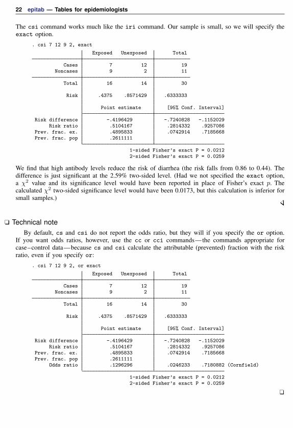
Example 6: csi
We have data on diarrhea during a 10-day follow-up period among 30 breast-fed infants colonizedwith Vibrio cholerae 01 according to antilipopolysaccharide antibody titers in the mother’s breastmilk (Glass et al. [1983]; reported in Rothman, Greenland, and Lash [2008, 248]):
Antibody levelHigh Low
Diarrhea 7 12No diarrhea 9 2
22 epitab — Tables for epidemiologists
The csi command works much like the iri command. Our sample is small, so we will specify theexact option.
. csi 7 12 9 2, exact
Exposed Unexposed Total
Cases 7 12 19Noncases 9 2 11
Total 16 14 30
Risk .4375 .8571429 .6333333
Point estimate [95% Conf. Interval]
Risk difference -.4196429 -.7240828 -.1152029Risk ratio .5104167 .2814332 .9257086
Prev. frac. ex. .4895833 .0742914 .7185668Prev. frac. pop .2611111
1-sided Fisher’s exact P = 0.02122-sided Fisher’s exact P = 0.0259
We find that high antibody levels reduce the risk of diarrhea (the risk falls from 0.86 to 0.44). Thedifference is just significant at the 2.59% two-sided level. (Had we not specified the exact option,a χ2 value and its significance level would have been reported in place of Fisher’s exact p. Thecalculated χ2 two-sided significance level would have been 0.0173, but this calculation is inferior forsmall samples.)
Technical noteBy default, cs and csi do not report the odds ratio, but they will if you specify the or option.
If you want odds ratios, however, use the cc or cci commands—the commands appropriate forcase–control data—because cs and csi calculate the attributable (prevented) fraction with the riskratio, even if you specify or:
. csi 7 12 9 2, or exact
Exposed Unexposed Total
Cases 7 12 19Noncases 9 2 11
Total 16 14 30
Risk .4375 .8571429 .6333333
Point estimate [95% Conf. Interval]
Risk difference -.4196429 -.7240828 -.1152029Risk ratio .5104167 .2814332 .9257086
Prev. frac. ex. .4895833 .0742914 .7185668Prev. frac. pop .2611111
Odds ratio .1296296 .0246233 .7180882 (Cornfield)
1-sided Fisher’s exact P = 0.02122-sided Fisher’s exact P = 0.0259

epitab — Tables for epidemiologists 23
Technical noteAs with iri and ir, csi and cs report either the attributable or the prevented fraction for the
exposed and total populations; see the discussion under Incidence-rate data above. In example 6, weestimated that 49% of potential cases in the exposed population were prevented by exposure. We alsoestimated that exposure accounted for a 26% reduction in cases over the entire population, but that isbased on the exposure distribution of the (small) population (16/30) and probably is of little interest.
Fleiss, Levin, and Paik (2003, 128) report infant mortality by birthweight for 72,730 live whitebirths in 1974 in New York City:
. csi 618 422 4597 67093
Exposed Unexposed Total
Cases 618 422 1040Noncases 4597 67093 71690
Total 5215 67515 72730
Risk .1185043 .0062505 .0142995
Point estimate [95% Conf. Interval]
Risk difference .1122539 .1034617 .121046Risk ratio 18.95929 16.80661 21.38769
Attr. frac. ex. .9472554 .9404996 .9532441Attr. frac. pop .5628883
chi2(1) = 4327.92 Pr>chi2 = 0.0000
In these data, exposed means a premature baby (birthweight ≤2,500 g), and a case is a baby who isdead at the end of one year. We find that being premature accounts for 94.7% of deaths among thepremature population. We also estimate, paraphrasing from Fleiss, Levin, and Paik (2003, 128), that56.3% of all white infant deaths in New York City in 1974 could have been prevented if prematurityhad been eliminated. (Moreover, Fleiss, Levin, and Paik put a standard error on the attributablefraction for the population. The formula is given in Methods and formulas but is appropriate onlyfor the population on which the estimates are based because other populations may have differentprobabilities of exposure.)
Example 7: cs
cs works like csi, except that it obtains its information from the data. The data equivalent totyping csi 7 12 9 2 are
. use http://www.stata-press.com/data/r15/csxmpl, clear
. list
case exp pop
1. 1 1 72. 1 0 123. 0 1 94. 0 0 2
We could then type cs case exp [freq=pop]. If we had individual-level data, so that each observationreflected a patient and we had 30 observations, we would type cs case exp.
24 epitab — Tables for epidemiologists
Stratified cumulative incidence data
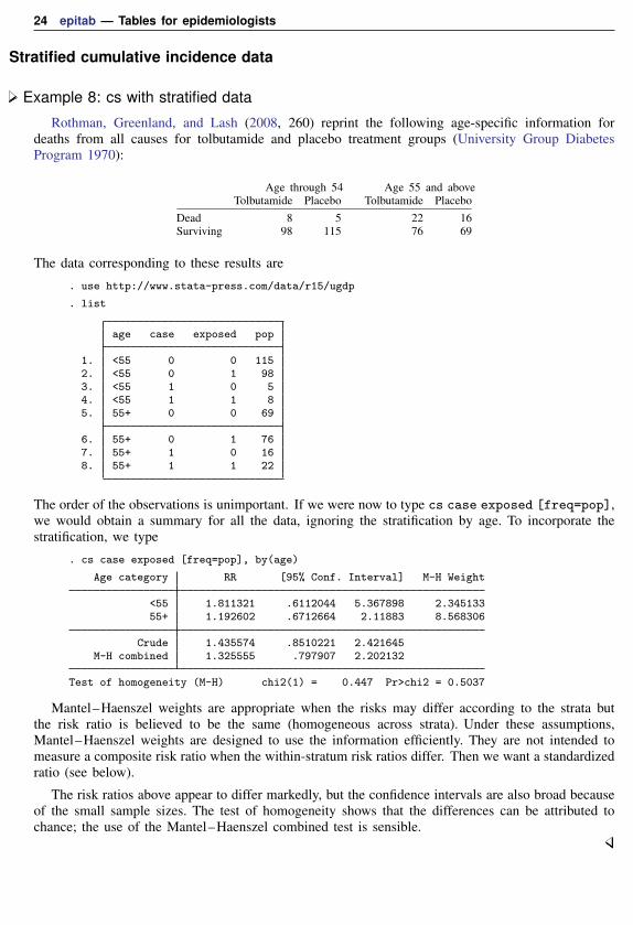
Example 8: cs with stratified data
Rothman, Greenland, and Lash (2008, 260) reprint the following age-specific information fordeaths from all causes for tolbutamide and placebo treatment groups (University Group DiabetesProgram 1970):
Age through 54 Age 55 and aboveTolbutamide Placebo Tolbutamide Placebo
Dead 8 5 22 16Surviving 98 115 76 69
The data corresponding to these results are
. use http://www.stata-press.com/data/r15/ugdp
. list
age case exposed pop
1. <55 0 0 1152. <55 0 1 983. <55 1 0 54. <55 1 1 85. 55+ 0 0 69
6. 55+ 0 1 767. 55+ 1 0 168. 55+ 1 1 22
The order of the observations is unimportant. If we were now to type cs case exposed [freq=pop],we would obtain a summary for all the data, ignoring the stratification by age. To incorporate thestratification, we type
. cs case exposed [freq=pop], by(age)
Age category RR [95% Conf. Interval] M-H Weight
<55 1.811321 .6112044 5.367898 2.34513355+ 1.192602 .6712664 2.11883 8.568306
Crude 1.435574 .8510221 2.421645M-H combined 1.325555 .797907 2.202132
Test of homogeneity (M-H) chi2(1) = 0.447 Pr>chi2 = 0.5037
Mantel–Haenszel weights are appropriate when the risks may differ according to the strata butthe risk ratio is believed to be the same (homogeneous across strata). Under these assumptions,Mantel–Haenszel weights are designed to use the information efficiently. They are not intended tomeasure a composite risk ratio when the within-stratum risk ratios differ. Then we want a standardizedratio (see below).
The risk ratios above appear to differ markedly, but the confidence intervals are also broad becauseof the small sample sizes. The test of homogeneity shows that the differences can be attributed tochance; the use of the Mantel–Haenszel combined test is sensible.

epitab — Tables for epidemiologists 25
Technical noteStratified cumulative incidence tables are not the only way to control for confounding. Another
way is logistic regression. However, logistic regression measures effects with odds ratios, not withrisk ratios. So before we fit a logistic model, let’s use cs to estimate the Mantel–Haenszel odds ratio:
. cs case exposed [freq=pop], by(age) or
Age category OR [95% Conf. Interval] M-H Weight
<55 1.877551 .6238165 5.637046 2.168142 (Cornfield)55+ 1.248355 .6112772 2.547411 6.644809 (Cornfield)
Crude 1.510673 .8381198 2.722012M-H combined 1.403149 .7625152 2.582015
Test of homogeneity (M-H) chi2(1) = 0.347 Pr>chi2 = 0.5556
Test that combined OR = 1:Mantel-Haenszel chi2(1) = 1.19
Pr>chi2 = 0.2750
The Mantel–Haenszel odds ratio is 1.40. It measures the association between death and treatmentwhile adjusting for age. A more general way to adjust for age is logistic regression; the outcomevariable is case, and it is explained by age and exposed. (As in the incidence-rate example, agemay appear to be a string variable in our data—we listed the data in the previous example—but itis actually a numeric variable taking on values 0 and 1 with value labels disguising that fact; see[U] 12.6.3 Value labels.)
. logistic case exposed age [freq=pop]
Logistic regression Number of obs = 409LR chi2(2) = 22.47Prob > chi2 = 0.0000
Log likelihood = -142.6212 Pseudo R2 = 0.0730
case Odds Ratio Std. Err. z P>|z| [95% Conf. Interval]
exposed 1.404674 .4374454 1.09 0.275 .7629451 2.586175age 4.216299 1.431519 4.24 0.000 2.167361 8.202223
_cons .0513818 .0170762 -8.93 0.000 .0267868 .0985593
Note: _cons estimates baseline odds.
Compare these results with the Mantel–Haenszel estimates obtained with cs:
Source Odds Ratio 95% Conf. Int.Mantel–Haenszel (cs) 1.40 0.76 2.58logistic 1.40 0.76 2.59
They are virtually identical.
Logistic regression has advantages over the stratified-table approach. First, we obtained an estimateof the age effect: being 55 years or over significantly increases the odds of death. In addition to thepoint estimate, 4.22, we have a confidence interval for the effect: 2.17 to 8.20.
A discrete effect at age 55 is not a plausible model of aging. It would be more reasonable toassume that a 54-year-old patient has a higher probability of death, due merely to age, than does a53-year-old patient; a 53-year-old, a higher probability than a 52-year-old patient; and so on. If wehad the underlying data, where each patient’s age is presumably known, we could include the actualage in the model and so better control for the age effect. This would improve our estimate of theeffect of being exposed to tolbutamide.

26 epitab — Tables for epidemiologists
See [R] logistic for an explanation of the logistic command. Also see the technical note inStratified incidence-rate data concerning categorical variables, which applies to logistic regression aswell as Poisson regression.
Standardized estimates with stratified cumulative incidence dataAs with ir, cs can produce standardized estimates, and the method is basically the same, although
the options for which estimates are to be combined or standardized make it confusing. We showedabove that cs can produce Mantel–Haenszel weighted estimates of the risk ratio (the default) or theodds ratio (obtained by specifying or). cs can also produce standardized estimates of the risk ratio(the default) or the risk difference (obtained by specifying rd).
Example 9: cs with stratified data, using standardized estimates
To produce an estimate of the internally standardized risk ratio by using our age-specific data ondeaths from all causes for tolbutamide and placebo treatment groups (example above), we type
. cs case exposed [freq=pop], by(age) istandard
Age category RR [95% Conf. Interval] Weight
<55 1.811321 .6112044 5.367898 10655+ 1.192602 .6712664 2.11883 98
Crude 1.435574 .8510221 2.421645I. Standardized 1.312122 .7889772 2.182147
We could obtain externally standardized estimates by substituting estandard for istandard.
To produce an estimate of the risk ratio weighting each age category equally, we could type
. generate wgt=1
. cs case exposed [freq=pop], by(age) standard(wgt)
Age category RR [95% Conf. Interval] Weight
<55 1.811321 .6112044 5.367898 155+ 1.192602 .6712664 2.11883 1
Crude 1.435574 .8510221 2.421645Standardized 1.304737 .7844994 2.169967
If we instead wanted the risk difference, we would type
. cs case exposed [freq=pop], by(age) standard(wgt) rd
Age category RD [95% Conf. Interval] Weight
<55 .033805 -.0278954 .0955055 155+ .0362545 -.0809204 .1534294 1
Crude .0446198 -.0192936 .1085332Standardized .0350298 -.0311837 .1012432
If we wanted to weight the less-than-55 age group five times as heavily as the 55-and-over group,we would create wgt to contain 5 for the first age group and 1 for the second (or 10 for the firstgroup and 2 for the second—the scale of the weights does not matter).
epitab — Tables for epidemiologists 27
Case–control dataIn case–control data, you select a sample on the basis of the outcome under study; that is, cases and
noncases are sampled at different rates. If you were examining the link between coffee consumptionand heart attacks, for instance, you could select a sample of subjects with and without the heartproblem and then examine their coffee-drinking behavior. A subject who has suffered a heart attack iscalled a case just as with cohort study data. A subject who has never suffered a heart attack, however,is called a control rather than merely a noncase, emphasizing that the sampling was performed withrespect to the outcome.
In case–control data, all hope of identifying the risk (that is, incidence) of the outcome (heartattacks) associated with the factor (coffee drinking) vanishes, at least without information on theunderlying sampling fractions, but you can examine the proportion of coffee drinkers among the twopopulations and reason that, if there is a difference, coffee drinking may be associated with the riskof heart attacks. Remarkably, even without the underlying sampling fractions, you can also measurethe ratio of the odds of heart attacks if a subject drinks coffee to the odds if a subject does not—theso-called odds ratio.
What is lost is the ability to compare absolute rates, which is not always the same as comparingrelative rates; see Fleiss, Levin, and Paik (2003, 123).
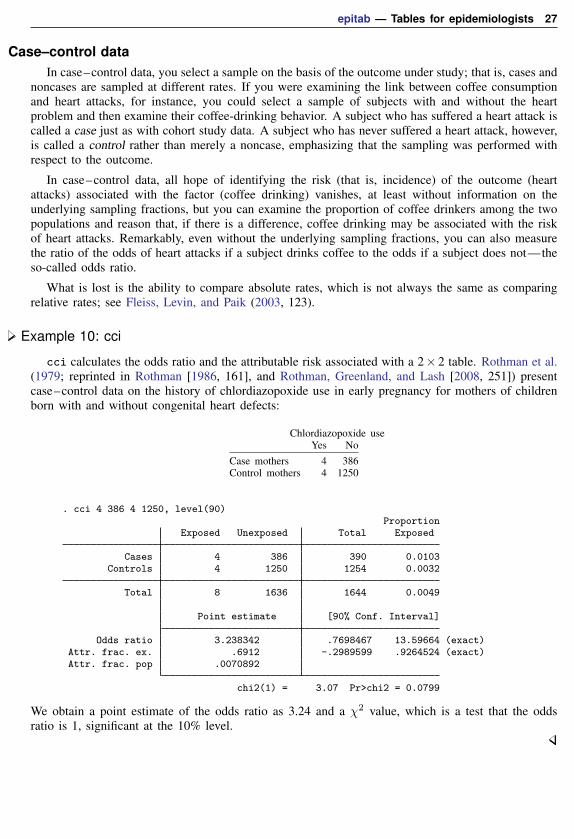
Example 10: cci
cci calculates the odds ratio and the attributable risk associated with a 2× 2 table. Rothman et al.(1979; reprinted in Rothman [1986, 161], and Rothman, Greenland, and Lash [2008, 251]) presentcase–control data on the history of chlordiazopoxide use in early pregnancy for mothers of childrenborn with and without congenital heart defects:
Chlordiazopoxide useYes No
Case mothers 4 386Control mothers 4 1250
. cci 4 386 4 1250, level(90)Proportion
Exposed Unexposed Total Exposed
Cases 4 386 390 0.0103Controls 4 1250 1254 0.0032
Total 8 1636 1644 0.0049
Point estimate [90% Conf. Interval]
Odds ratio 3.238342 .7698467 13.59664 (exact)Attr. frac. ex. .6912 -.2989599 .9264524 (exact)Attr. frac. pop .0070892
chi2(1) = 3.07 Pr>chi2 = 0.0799
We obtain a point estimate of the odds ratio as 3.24 and a χ2 value, which is a test that the oddsratio is 1, significant at the 10% level.

28 epitab — Tables for epidemiologists
Technical noteThe epitab commands can calculate three different confidence intervals for the odds ratio: the exact,
Woolf, and Cornfield intervals. The exact interval, illustrated in example 10, is the default. The intervalis “exact” because it uses an exact sampling distribution—a distribution with no unknown parametersunder the null hypothesis. An exact interval does not use a normal or chi-squared approximation.“Exact” does not describe the coverage probability; the coverage probability of a 90% exact intervalis not exactly 90%. The coverage probability is actually bounded below by 90% (Agresti 2013, 606),so a 90% exact interval will always cover the odds ratio with probability at least 90% (if the modelis correct).
The Woolf and Cornfield intervals, on the other hand, are approximate. They approximate theexact sampling distribution with a normal model and are not guaranteed to maintain their nominalcoverage: the coverage probability of a 90% approximate interval fluctuates above and below 90%.The coverage approaches 90% only in the limit as the sample size increases. Exact intervals areconservative; approximate intervals can be conservative or anticonservative (Agresti 2013, 607).
If you wish to maintain nominal coverage, then you should use the exact interval. But you willpay a price for the coverage: the exact interval will usually be wider than the approximate intervals.Example 10 is no exception:
Method 90% Conf. Int. Commandexact 0.77 13.60 cciWoolf 1.01 10.40 cci, woolfCornfield 1.07 9.83 cci, cornfield
The exact interval is the widest of the three—so wide that it includes the null value of one—eventhough the chi-squared p-value of 0.0799 was significant at the 10% level. The exact interval andchi-squared test come from different models, so we should not expect them to always agree on sharpconclusions such as statistical significance.
The odds-ratio intervals are all frequentist methods, so we cannot compare them rigorously withone example. See Brown (1981), Gart and Thomas (1982), and Agresti (1999) for more rigorouscomparisons. Agresti (1999) found that the Woolf interval performed well, even for small samples.
� �Jerome Cornfield (1912–1979) was born in New York City. He majored in history at New YorkUniversity and took courses in statistics at the U.S. Department of Agriculture Graduate Schoolbut otherwise had little formal training. Cornfield held positions at the Bureau of Labor Statistics,the National Cancer Institute, the National Institutes of Health, Johns Hopkins University, theUniversity of Pittsburgh, and George Washington University. He worked on many problems inbiomedical statistics, including the analysis of clinical trials, epidemiology (especially case–controlstudies), and Bayesian approaches.
Barnet Woolf (1902–1983) was born in London. His parents were immigrants from Lithuania.Woolf was educated at Cambridge, where he studied physiology and biochemistry, and proposedmethods for linearizing plots in enzyme chemistry that were later rediscovered by others (seeHaldane [1957]). His later career in London, Birmingham, Rothamsted, and Edinburgh includedlasting contributions to nutrition, epidemiology, public health, genetics, and statistics. He wasalso active in left-wing causes and penned humorous poems, songs, and revues.� �
epitab — Tables for epidemiologists 29
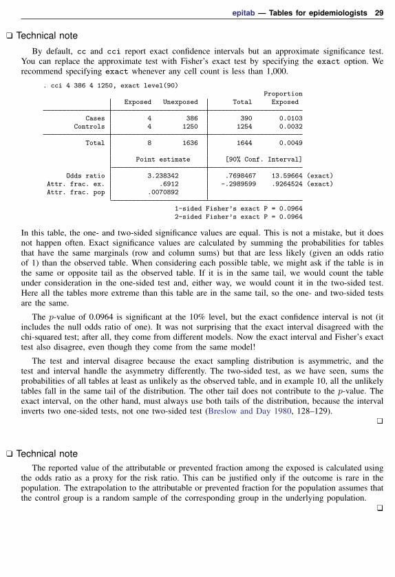
Technical note
By default, cc and cci report exact confidence intervals but an approximate significance test.You can replace the approximate test with Fisher’s exact test by specifying the exact option. Werecommend specifying exact whenever any cell count is less than 1,000.
. cci 4 386 4 1250, exact level(90)Proportion
Exposed Unexposed Total Exposed
Cases 4 386 390 0.0103Controls 4 1250 1254 0.0032
Total 8 1636 1644 0.0049
Point estimate [90% Conf. Interval]
Odds ratio 3.238342 .7698467 13.59664 (exact)Attr. frac. ex. .6912 -.2989599 .9264524 (exact)Attr. frac. pop .0070892
1-sided Fisher’s exact P = 0.09642-sided Fisher’s exact P = 0.0964
In this table, the one- and two-sided significance values are equal. This is not a mistake, but it doesnot happen often. Exact significance values are calculated by summing the probabilities for tablesthat have the same marginals (row and column sums) but that are less likely (given an odds ratioof 1) than the observed table. When considering each possible table, we might ask if the table is inthe same or opposite tail as the observed table. If it is in the same tail, we would count the tableunder consideration in the one-sided test and, either way, we would count it in the two-sided test.Here all the tables more extreme than this table are in the same tail, so the one- and two-sided testsare the same.
The p-value of 0.0964 is significant at the 10% level, but the exact confidence interval is not (itincludes the null odds ratio of one). It was not surprising that the exact interval disagreed with thechi-squared test; after all, they come from different models. Now the exact interval and Fisher’s exacttest also disagree, even though they come from the same model!
The test and interval disagree because the exact sampling distribution is asymmetric, and thetest and interval handle the asymmetry differently. The two-sided test, as we have seen, sums theprobabilities of all tables at least as unlikely as the observed table, and in example 10, all the unlikelytables fall in the same tail of the distribution. The other tail does not contribute to the p-value. Theexact interval, on the other hand, must always use both tails of the distribution, because the intervalinverts two one-sided tests, not one two-sided test (Breslow and Day 1980, 128–129).
Technical noteThe reported value of the attributable or prevented fraction among the exposed is calculated using
the odds ratio as a proxy for the risk ratio. This can be justified only if the outcome is rare in thepopulation. The extrapolation to the attributable or prevented fraction for the population assumes thatthe control group is a random sample of the corresponding group in the underlying population.

30 epitab — Tables for epidemiologists
Example 11: cc equivalent to cci
Equivalent to typing cci 4 386 4 1250 would be typing cc case exposed [freq=pop] withthe following data:
. use http://www.stata-press.com/data/r15/ccxmpl, clear
. list
case exposed pop
1. 1 1 42. 1 0 3863. 0 1 44. 0 0 1250
Stratified case–control data
Example 12: cc with stratified data
cc can work with stratified tables. Rothman, Greenland, and Lash (2008, 276) reprint and discussdata from a case–control study on infants with congenital heart disease and Down syndrome andhealthy controls, according to maternal spermicide use before conception and maternal age at delivery(Rothman 1982):
Maternal age to 34 Maternal age 35+Spermicide used not used Spermicide used not used
Down syndrome 3 9 1 3Controls 104 1059 5 86
The data corresponding to these tables are
. use http://www.stata-press.com/data/r15/downs
. list
case exposed pop age
1. 1 1 3 <352. 1 0 9 <353. 0 1 104 <354. 0 0 1059 <355. 1 1 1 35+
6. 1 0 3 35+7. 0 1 5 35+8. 0 0 86 35+

epitab — Tables for epidemiologists 31
The stratified results for the odds ratio are
. cc case exposed [freq=pop], by(age) woolf
Maternal age OR [95% Conf. Interval] M-H Weight
<35 3.394231 .9048403 12.73242 .7965957 (Woolf)35+ 5.733333 .5016418 65.52706 .1578947 (Woolf)
Crude 3.501529 1.110362 11.04208 (Woolf)M-H combined 3.781172 1.18734 12.04142
Test of homogeneity (M-H) chi2(1) = 0.14 Pr>chi2 = 0.7105
Test that combined OR = 1:Mantel-Haenszel chi2(1) = 5.81
Pr>chi2 = 0.0159
For no particular reason, we also specified the woolf option to obtain Woolf approximations tothe within-stratum confidence intervals rather than the default. Had we wanted Tarone’s test ofhomogeneity, we would have used
. cc case exposed [freq=pop], by(age) tarone
Maternal age OR [95% Conf. Interval] M-H Weight
<35 3.394231 .5812415 13.87412 .7965957 (exact)35+ 5.733333 .0911619 85.89602 .1578947 (exact)
Crude 3.501529 .8080857 11.78958 (exact)M-H combined 3.781172 1.18734 12.04142
Test of homogeneity (M-H) chi2(1) = 0.14 Pr>chi2 = 0.7105Test of homogeneity (Tarone) chi2(1) = 0.14 Pr>chi2 = 0.7092
Test that combined OR = 1:Mantel-Haenszel chi2(1) = 5.81
Pr>chi2 = 0.0159
Whatever method you choose for calculating confidence intervals, Stata will report a test ofhomogeneity, which here is χ2(1) = 0.14 and not significant. That is, the odds of Down syndromemight vary with maternal age, but we cannot reject the hypothesis that the association between Downsyndrome and spermicide is the same in the two maternal age strata. This is thus a test to reject theappropriateness of the single, Mantel–Haenszel combined odds ratio—a rejection not justified bythese data.
Technical noteThe cc command includes four tests of homogeneity: Mantel–Haenszel (the default); directly
pooled, also known as the Woolf test (available with the pool option); Tarone (available with thetarone option); and Breslow–Day (available with the bd option). The preferred test is Tarone’s(Tarone 1985, 94), which corrected an error in the Breslow–Day test; see Breslow (1996, 17–18) fordetails of the error and Tarone’s correction.
The other two homogeneity tests, the Mantel–Haenszel and directly pooled, are less useful: theyuse the logs of the stratum-specific odds ratios, so they are undefined when any stratum has a zerocell. The epitab commands deal with the problem differently: cs omits the offending strata, whilecc substitutes the Tarone test. The Tarone test does not use the stratum-specific odds ratios, so it canstill be calculated when there are zero cells.

32 epitab — Tables for epidemiologists
None of the tests are appropriate for finely stratified (many strata with only a few observations each)studies (Rothman, Greenland, and Lash 2008, 280). If you have fine stratification, one alternative ismultilevel logistic regression; see [ME] melogit.
Technical noteAs with cohort study data, an alternative to stratified tables for uncovering effects is logistic
regression. From the logistic point of view, case–control data are no different from cohort studydata—you must merely ignore the estimated intercept. The intercept is meaningless in case–controldata because it reflects the baseline prevalence of the outcome, which you controlled by sampling.
The data we used with cc can be used directly by logistic. (The age variable, which appearsto be a string, is really numeric with an associated value label; see [U] 12.6.3 Value labels. age takeson the value 0 for the age-less-than-35 group and 1 for the 35+ group.)
. logistic case exposed age [freq=pop]
Logistic regression Number of obs = 1,270LR chi2(2) = 8.74Prob > chi2 = 0.0127
Log likelihood = -81.517532 Pseudo R2 = 0.0509
case Odds Ratio Std. Err. z P>|z| [95% Conf. Interval]
exposed 3.787779 2.241922 2.25 0.024 1.187334 12.0836age 4.582857 2.717352 2.57 0.010 1.433594 14.65029
_cons .0082631 .0027325 -14.50 0.000 .0043218 .0157988
Note: _cons estimates baseline odds.
We compare the results with those presented by cc in the previous example:
Source Odds ratio 95% CIMantel–Haenszel (cc) 3.78 1.19 12.04logistic 3.79 1.19 12.08
As with the cohort study data in example 8, results are virtually identical, and all the same commentswe made previously apply once again.
To demonstrate an advantage of logistic regression, let’s now ask a question that would be difficultto answer on the basis of a stratified table analysis. We now know that spermicide use appears toincrease the risk of having a baby with Down syndrome, and we know that the mother’s age alsoincreases the risk. Is the effect of spermicide use statistically different for mothers in the two agegroups?

epitab — Tables for epidemiologists 33
. logistic case exposed age c.age#exposed [freq=pop]
Logistic regression Number of obs = 1,270LR chi2(3) = 8.87Prob > chi2 = 0.0311
Log likelihood = -81.451332 Pseudo R2 = 0.0516
case Odds Ratio Std. Err. z P>|z| [95% Conf. Interval]
exposed 3.394231 2.289544 1.81 0.070 .9048403 12.73242age 4.104651 2.774868 2.09 0.037 1.091034 15.44237
exposed#c.age1 1.689141 2.388785 0.37 0.711 .1056563 27.0045
_cons .0084986 .0028449 -14.24 0.000 .0044097 .0163789
Note: _cons estimates baseline odds.
The answer is no. The odds ratio and confidence interval reported for exposed now measure thespermicide effect for an age==0 (age < 35) mother. The odds ratio and confidence interval reportedfor c.age#exposed are the (multiplicative) difference in the spermicide odds ratio for an age==1(age 35+) mother relative to a young mother. The point estimate is that the effect is larger for oldermothers, suggesting grounds for future research, but the difference is not significant.
See [R] logistic for an explanation of the logistic command. Also see the technical note underIncidence-rate data above concerning Poisson regression, which applies equally to logistic regression.
Case–control data with multiple levels of exposure
In a case–control study, subjects with the disease of interest (cases) are compared to disease-freeindividuals (controls) to assess the relationship between exposure to one or more risk factors anddisease incidence. Often exposure is measured qualitatively at several discrete levels or measured ona continuous scale and then grouped into three or more levels. The data can be summarized as
Exposure level1 2 . . . k Total
Cases a1 a2 . . . ak M1
Controls c1 c2 . . . ck M0
Total N1 N2 . . . Nk T
An advantage afforded by having multiple levels of exposure is the ability to examine dose–responserelationships. If the association between a risk factor and a disease or outcome is real, we expectthe strength of that association to increase with the level and duration of exposure. A dose–responserelationship provides strong support for a direct or even causal relationship between the risk factorand the outcome. On the other hand, the lack of a dose–response is usually seen as an argumentagainst causality.
We can use the tabodds command to tabulate the odds of failure or odds ratios against a categoricalexposure variable. The test for trend calculated by tabodds can serve as a test for dose–response ifthe exposure variable is at least ordinal. If the exposure variable has no natural ordering, the trendtest is meaningless and should be ignored. See the technical note at the end of this section for moreinformation regarding the test for trend.

34 epitab — Tables for epidemiologists
Before looking at an example, consider three possible data arrangements for case–control andprevalence studies. The most common data arrangement is individual records, where each subject inthe study has his or her own record. Closely related are frequency records where identical individualrecords are included only once, but with a variable giving the frequency with which the record occurs.The fweight weight option is used for these data to specify the frequency variable. Data can alsobe arranged as binomial frequency records where each record contains a variable, D, the number ofcases; another variable, N, the number of total subjects (cases plus controls); and other variables. Anadvantage of binomial frequency records is that large datasets can be entered succinctly into a Statadatabase.
Example 13: tabodds
Consider the following data from the Ille-et-Vilaine study of esophageal cancer, discussed inBreslow and Day (1980, chap. 4 and app. I), corresponding to subjects age 55–64 who use from 0to 9 g of tobacco per day:
Alcohol consumption (g/day)0–39 40–79 80–119 120+ Total
Cases 2 9 9 5 25Controls 47 31 9 5 92Total 49 40 18 10 117
The study included 24 such tables, each representing one of four levels of tobacco use and one ofsix age categories. We can create a binomial frequency-record dataset by typing
. input alcohol D N agegrp tobacco
alcohol D N agegrp tobacco1. 1 2 49 4 12. 2 9 40 4 13. 3 9 18 4 14. 4 5 10 4 15. end
where D is the number of esophageal cancer cases and N is the number of total subjects (cases pluscontrols) for each combination of six age groups (agegrp), four levels of alcohol consumption ing/day (alcohol), and four levels of tobacco use in g/day (tobacco).
Both the tabodds and mhodds commands can correctly handle all three data arrangements.Binomial frequency records require that the number of total subjects (cases plus controls) representedby each record N be specified with the binomial() option.
We could also enter the data as frequency-weighted data:
. input alcohol case freq agegrp tobacco
alcohol case freq agegrp tobacco1. 1 1 2 4 12. 1 0 47 4 13. 2 1 9 4 14. 2 0 31 4 15. 3 1 9 4 16. 3 0 9 4 17. 4 1 5 4 18. 4 0 5 4 19. end

epitab — Tables for epidemiologists 35
If you are planning on using any of the other estimation commands, such as poisson or logistic,we recommend that you enter your data either as individual records or as frequency-weighted recordsand not as binomial frequency records, because the estimation commands currently do not recognizethe binomial() option.
We have entered all the esophageal cancer data into Stata as a frequency-weighted record datasetas previously described. In our data, case indicates the esophageal cancer cases and controls, andfreq is the number of subjects represented by each record (the weight).
We added value labels to the agegrp, alcohol, and tobacco variables in our dataset to easeinterpretation in outputs, but these variables are numeric.
We are interested in the association between alcohol consumption and esophageal cancer. We firstuse tabodds to tabulate the odds of esophageal cancer against alcohol consumption:
. use http://www.stata-press.com/data/r15/bdesop, clear
. tabodds case alcohol [fweight=freq]
alcohol cases controls odds [95% Conf. Interval]
0-39 29 386 0.07513 0.05151 0.1095740-79 75 280 0.26786 0.20760 0.34560
80-119 51 87 0.58621 0.41489 0.82826120+ 45 22 2.04545 1.22843 3.40587
Test of homogeneity (equal odds): chi2(3) = 158.79Pr>chi2 = 0.0000
Score test for trend of odds: chi2(1) = 152.97Pr>chi2 = 0.0000
The test of homogeneity clearly indicates that the odds of esophageal cancer differ by level of alcoholconsumption, and the test for trend indicates a significant increase in odds with increasing alcoholuse. This suggests a strong dose–response relation. The graph option can be used to study the shapeof the relationship of the odds with alcohol consumption. Most of the heterogeneity in these datacan be “explained” by the linear increase in risk of esophageal cancer with increased dosage (alcoholconsumption).
We also could have requested that the odds ratios at each level of alcohol consumption be calculatedby specifying the or option. For example, tabodds case alcohol [fweight=freq], or wouldproduce odds ratios using the minimum value of alcohol—that is, alcohol = 1 (0–39)—as thereference group, and the command tabodds case alcohol [fweight=freq], or base(2) woulduse alcohol = 2 (40–79) as the reference group.
Although our results appear to provide strong evidence supporting an association between alcoholconsumption and esophageal cancer, we need to be concerned with the possible existence of confounders,specifically age and tobacco use, in our data. We can again use tabodds to tabulate the odds ofesophageal cancer against age and against tobacco use, independently:
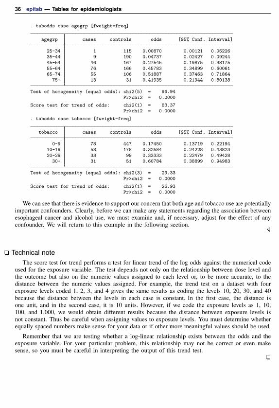
36 epitab — Tables for epidemiologists
. tabodds case agegrp [fweight=freq]
agegrp cases controls odds [95% Conf. Interval]
25-34 1 115 0.00870 0.00121 0.0622635-44 9 190 0.04737 0.02427 0.0924445-54 46 167 0.27545 0.19875 0.3817555-64 76 166 0.45783 0.34899 0.6006165-74 55 106 0.51887 0.37463 0.71864
75+ 13 31 0.41935 0.21944 0.80138
Test of homogeneity (equal odds): chi2(5) = 96.94Pr>chi2 = 0.0000
Score test for trend of odds: chi2(1) = 83.37Pr>chi2 = 0.0000
. tabodds case tobacco [fweight=freq]
tobacco cases controls odds [95% Conf. Interval]
0-9 78 447 0.17450 0.13719 0.2219410-19 58 178 0.32584 0.24228 0.4382320-29 33 99 0.33333 0.22479 0.49428
30+ 31 51 0.60784 0.38899 0.94983
Test of homogeneity (equal odds): chi2(3) = 29.33Pr>chi2 = 0.0000
Score test for trend of odds: chi2(1) = 26.93Pr>chi2 = 0.0000
We can see that there is evidence to support our concern that both age and tobacco use are potentiallyimportant confounders. Clearly, before we can make any statements regarding the association betweenesophageal cancer and alcohol use, we must examine and, if necessary, adjust for the effect of anyconfounder. We will return to this example in the following section.
Technical noteThe score test for trend performs a test for linear trend of the log odds against the numerical code
used for the exposure variable. The test depends not only on the relationship between dose level andthe outcome but also on the numeric values assigned to each level or, to be more accurate, to thedistance between the numeric values assigned. For example, the trend test on a dataset with fourexposure levels coded 1, 2, 3, and 4 gives the same results as coding the levels 10, 20, 30, and 40because the distance between the levels in each case is constant. In the first case, the distance isone unit, and in the second case, it is 10 units. However, if we code the exposure levels as 1, 10,100, and 1,000, we would obtain different results because the distance between exposure levels isnot constant. Thus be careful when assigning values to exposure levels. You must determine whetherequally spaced numbers make sense for your data or if other more meaningful values should be used.
Remember that we are testing whether a log-linear relationship exists between the odds and theexposure variable. For your particular problem, this relationship may not be correct or even makesense, so you must be careful in interpreting the output of this trend test.

epitab — Tables for epidemiologists 37
Case–control data with confounders and possibly multiple levels of exposure
In the esophageal cancer data example introduced earlier, we determined that the apparent associationbetween alcohol consumption and esophageal cancer could be confounded by age and tobacco use.You can adjust for the effect of possible confounding factors by stratifying on these factors. This isthe method used by both tabodds and mhodds to adjust for other variables in the dataset. We willcompare and contrast these two commands in the following example.
Example 14: tabodds, adjusting for confounding factors
We begin by using tabodds to tabulate unadjusted odds ratios.
. tabodds case alcohol [fweight=freq], or
alcohol Odds Ratio chi2 P>chi2 [95% Conf. Interval]
0-39 1.000000 . . . .40-79 3.565271 32.70 0.0000 2.237981 5.679744
80-119 7.802616 75.03 0.0000 4.497054 13.537932120+ 27.225705 160.41 0.0000 12.507808 59.262107
Test of homogeneity (equal odds): chi2(3) = 158.79Pr>chi2 = 0.0000
Score test for trend of odds: chi2(1) = 152.97Pr>chi2 = 0.0000
The alcohol = 1 group (0–39) was used by tabodds as the reference category for calculatingthe odds ratios. We could have selected a different group by specifying the base() option; however,because the lowest dosage level is most often the appropriate reference group, as it is in these data,the base() option is seldom used.
We use tabodds with the adjust() option to tabulate Mantel–Haenszel age-adjusted odds ratios:
. tabodds case alcohol [fweight=freq], adjust(age)
Mantel-Haenszel odds ratios adjusted for age
alcohol Odds Ratio chi2 P>chi2 [95% Conf. Interval]
0-39 1.000000 . . . .40-79 4.268155 37.36 0.0000 2.570025 7.088314
80-119 8.018305 59.30 0.0000 4.266893 15.067922120+ 28.570426 139.70 0.0000 12.146409 67.202514
Score test for trend of odds: chi2(1) = 135.09Pr>chi2 = 0.0000
We observe that the age-adjusted odds ratios are just slightly higher than the unadjusted ones, so itappears that age is not as strong a confounder as it first appeared. Even after adjusting for age, thedose–response relationship, as measured by the trend test, remains strong.
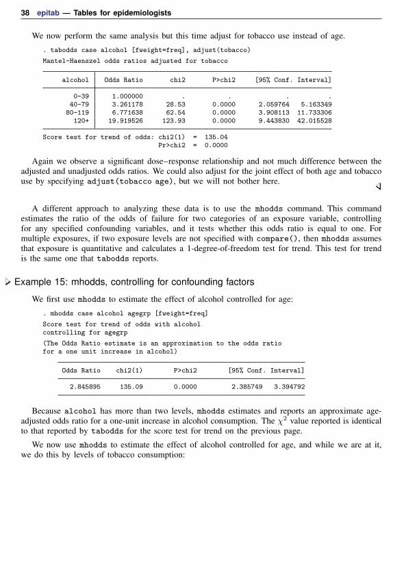
38 epitab — Tables for epidemiologists
We now perform the same analysis but this time adjust for tobacco use instead of age.
. tabodds case alcohol [fweight=freq], adjust(tobacco)
Mantel-Haenszel odds ratios adjusted for tobacco
alcohol Odds Ratio chi2 P>chi2 [95% Conf. Interval]
0-39 1.000000 . . . .40-79 3.261178 28.53 0.0000 2.059764 5.163349
80-119 6.771638 62.54 0.0000 3.908113 11.733306120+ 19.919526 123.93 0.0000 9.443830 42.015528
Score test for trend of odds: chi2(1) = 135.04Pr>chi2 = 0.0000
Again we observe a significant dose–response relationship and not much difference between theadjusted and unadjusted odds ratios. We could also adjust for the joint effect of both age and tobaccouse by specifying adjust(tobacco age), but we will not bother here.
A different approach to analyzing these data is to use the mhodds command. This commandestimates the ratio of the odds of failure for two categories of an exposure variable, controllingfor any specified confounding variables, and it tests whether this odds ratio is equal to one. Formultiple exposures, if two exposure levels are not specified with compare(), then mhodds assumesthat exposure is quantitative and calculates a 1-degree-of-freedom test for trend. This test for trendis the same one that tabodds reports.
Example 15: mhodds, controlling for confounding factors
We first use mhodds to estimate the effect of alcohol controlled for age:
. mhodds case alcohol agegrp [fweight=freq]
Score test for trend of odds with alcoholcontrolling for agegrp
(The Odds Ratio estimate is an approximation to the odds ratiofor a one unit increase in alcohol)
Odds Ratio chi2(1) P>chi2 [95% Conf. Interval]
2.845895 135.09 0.0000 2.385749 3.394792
Because alcohol has more than two levels, mhodds estimates and reports an approximate age-adjusted odds ratio for a one-unit increase in alcohol consumption. The χ2 value reported is identicalto that reported by tabodds for the score test for trend on the previous page.
We now use mhodds to estimate the effect of alcohol controlled for age, and while we are at it,we do this by levels of tobacco consumption:
epitab — Tables for epidemiologists 39
. mhodds case alcohol agegrp [fweight=freq], by(tobacco)
Score test for trend of odds with alcoholcontrolling for agegrpby tobacco
note: only 19 of the 24 strata formed in this analysis contributeinformation about the effect of the explanatory variable
(The Odds Ratio estimate is an approximation to the odds ratiofor a one unit increase in alcohol)
tobacco Odds Ratio chi2(1) P>chi2 [95% Conf. Interval]
0-9 3.579667 75.95 0.0000 2.68710 4.7687110-19 2.303580 25.77 0.0000 1.66913 3.1792020-29 2.364135 13.27 0.0003 1.48810 3.75589
30+ 2.217946 8.84 0.0029 1.31184 3.74992
Mantel-Haenszel estimate controlling for agegrp and tobacco
Odds Ratio chi2(1) P>chi2 [95% Conf. Interval]
2.751236 118.37 0.0000 2.292705 3.301471
Test of homogeneity of ORs (approx): chi2(3) = 5.46Pr>chi2 = 0.1409
Again, because alcohol has more than two levels, mhodds estimates and reports an approximateMantel–Haenszel age and tobacco-use adjusted odds ratio for a one-unit increase in alcohol con-sumption. The χ2 test for trend reported with the Mantel–Haenszel estimate is again the same onethat tabodds produces if adjust(agegrp tobacco) is specified.
The results from this analysis also show an effect of alcohol, controlled for age, of about ×2.7,which is consistent across different levels of tobacco consumption. Similarly,
. mhodds case tobacco agegrp [fweight=freq], by(alcohol)
Score test for trend of odds with tobaccocontrolling for agegrpby alcohol
note: only 18 of the 24 strata formed in this analysis contributeinformation about the effect of the explanatory variable
(The Odds Ratio estimate is an approximation to the odds ratiofor a one unit increase in tobacco)
alcohol Odds Ratio chi2(1) P>chi2 [95% Conf. Interval]
0-39 2.420650 15.61 0.0001 1.56121 3.7532040-79 1.427713 5.75 0.0165 1.06717 1.91007
80-119 1.472218 3.38 0.0659 0.97483 2.22339120+ 1.214815 0.59 0.4432 0.73876 1.99763
Mantel-Haenszel estimate controlling for agegrp and alcohol
Odds Ratio chi2(1) P>chi2 [95% Conf. Interval]
1.553437 20.07 0.0000 1.281160 1.883580
Test of homogeneity of ORs (approx): chi2(3) = 5.26Pr>chi2 = 0.1540

40 epitab — Tables for epidemiologists
shows an effect of tobacco, controlled for age, of about ×1.5, which is consistent across differentlevels of alcohol consumption.
Comparisons between particular levels of alcohol and tobacco consumption can be made bygenerating a new variable with levels corresponding to all combinations of alcohol and tobacco, as in
. egen alctob = group(alcohol tobacco)
. mhodds case alctob [fweight=freq], compare(16,1)
Maximum likelihood estimate of the odds ratioComparing alctob==16 vs. alctob==1
Odds Ratio chi2(1) P>chi2 [95% Conf. Interval]
93.333333 103.21 0.0000 14.766136 589.938431
which yields an odds ratio of 93 between subjects with the highest levels of alcohol and tobacco andthose with the lowest levels. Similar results can be obtained simultaneously for all levels of alctobusing alctob = 1 as the comparison group by specifying tabodds D alctob, bin(N) or.
Standardized estimates with stratified case–control data
Example 16: cc with stratified data, using standardized estimates
You obtain standardized estimates (here for the odds ratio) by using cc just as you obtain standardizedestimates by using ir or cs. Along with the by() option, you specify one of estandard, istandard,or standard(varname).
Case–control studies can provide standardized rate-ratio estimates when density sampling is used,or when the disease is rare (Rothman, Greenland, and Lash 2008, 269). Rothman, Greenland, andLash (2008, 276) report the SMR for the case–control study on infants with congenital heart diseaseand Down syndrome. We can reproduce their estimates along with the pooled estimates by typing
. use http://www.stata-press.com/data/r15/downs, clear
. cc case exposed [freq=pop], by(age) istandard pool
Maternal age OR [95% Conf. Interval] Weight
<35 3.394231 .5812415 13.87412 104 (exact)35+ 5.733333 .0911619 85.89602 5 (exact)
Crude 3.501529 .8080857 11.78958 (exact)Pooled (direct) 3.824166 1.196437 12.22316I. Standardized 3.779749 1.180566 12.10141
Test of homogeneity (direct) chi2(1) = 0.14 Pr>chi2 = 0.7109
Using the distribution of the nonexposed subjects in the source population as the standard, we canobtain an estimate of the standardized rate ratio (SRR):
. cc case exposed [freq=pop], by(age) estandard
Maternal age OR [95% Conf. Interval] Weight
<35 3.394231 .5812415 13.87412 1059 (exact)35+ 5.733333 .0911619 85.89602 86 (exact)
Crude 3.501529 .8080857 11.78958 (exact)E. Standardized 3.979006 1.176096 13.46191

epitab — Tables for epidemiologists 41
Finally, if we wanted to weight the two age groups equally, we could type
. generate wgt=1
. cc case exposed [freq=pop], by(age) standard(wgt)
Maternal age OR [95% Conf. Interval] Weight
<35 3.394231 .5812415 13.87412 1 (exact)35+ 5.733333 .0911619 85.89602 1 (exact)
Crude 3.501529 .8080857 11.78958 (exact)Standardized 5.275104 .6233794 44.6385
Matched case–control dataMatched case–control studies are performed to gain sample-size efficiency and to control for
important confounding factors. In a matched case–control design, each case is matched with a controlon the basis of demographic characteristics, clinical characteristics, etc. Thus their difference withrespect to the outcome must be due to something other than the matching variables. If the onlydifference between them was exposure to the factor, we could attribute any difference in outcome tothe factor.
A summary of the data is
ControlsCases Exposed Unexposed Total
Exposed a b M1
Unexposed c d M0
Total N1 N0 T = a+ b+ c+ d
Each entry in the table represents the number of case–control pairs. For instance, in a of the pairs,both members were exposed; in b of the pairs, the case was exposed but the control was not; and soon. In total, T pairs were observed.
Example 17: mcci
Rothman (1986, 257) discusses data from Jick et al. (1973) on a matched case–control study ofmyocardial infarction and drinking six or more cups of coffee per day (persons drinking from one tofive cups per day were excluded):
ControlsCases 6+ cups 0 cups
6+ cups 8 80 cups 3 8

42 epitab — Tables for epidemiologists
mcci analyzes matched case–control data:
. mcci 8 8 3 8
ControlsCases Exposed Unexposed Total
Exposed 8 8 16Unexposed 3 8 11
Total 11 16 27
McNemar’s chi2(1) = 2.27 Prob > chi2 = 0.1317Exact McNemar significance probability = 0.2266
Proportion with factorCases .5925926Controls .4074074 [95% Conf. Interval]
difference .1851852 -.0822542 .4526246ratio 1.454545 .891101 2.374257rel. diff. .3125 -.0243688 .6493688
odds ratio 2.666667 .6400364 15.6064 (exact)
The point estimate states that the odds of drinking 6 or more cups of coffee per day is 2.67 timesgreater among the myocardial infarction patients. The confidence interval is wide, however, and thep-value of 0.1317 from McNemar’s test is not statistically significant.
mcc works like the other nonimmediate commands but does not handle stratified data. If you havestratified matched case–control data, you can use conditional logistic regression to estimate oddsratios; see [R] clogit.
Matched case–control studies can also be analyzed using mhodds by controlling on the variableused to identify the matched sets. For example, if the variable set is used to identify the matchedset for each subject,
. mhodds fail xvar set
will do the job. Any attempt to control for further variables will restrict the analysis to the comparisonof cases and matched controls that share the same values of these variables. In general, this wouldlead to the omission of many records from the analysis. Similar considerations usually apply wheninvestigating effect modification by using the by() option. An important exception to this rule is thata variable used in matching cases to controls may appear in the by() option without loss of data.
Example 18: mhodds with matched case–control data
Let’s use mhodds to analyze matched case–control studies using the study of endometrial cancerand exposure to estrogen described in Breslow and Day (1980, chap. 5). In this study, there are fourcontrols matched to each case. Cases and controls are matched on age, marital status, and time livingin the community. The data collected include information on the daily dose of conjugated estrogentherapy. Breslow and Day created four levels of the dose variable and began by analyzing the 1:1study formed by using the first control in each set. We examine the effect of exposure to estrogen:
epitab — Tables for epidemiologists 43
. use http://www.stata-press.com/data/r15/bdendo11, clear
. describe
Contains data from http://www.stata-press.com/data/r15/bdendo11.dtaobs: 126
vars: 13 3 Mar 2016 23:29size: 2,394
storage display valuevariable name type format label variable label
set int %8.0g Set numberfail byte %8.0g Case=1/Control=0gall byte %8.0g Gallbladder dishyp byte %8.0g Hypertensionob byte %8.0g Obesityest byte %8.0g Estrogendos byte %8.0g Ordinal dosedur byte %8.0g Ordinal durationnon byte %8.0g Non-estrogen drugduration int %8.0g monthsage int %8.0g yearscest byte %8.0g Conjugated est doseagegrp float %9.0g age group of set
Sorted by: set
. mhodds fail est set
Mantel-Haenszel estimate of the odds ratioComparing est==1 vs. est==0, controlling for set
note: only 32 of the 63 strata formed in this analysis contributeinformation about the effect of the explanatory variable
Odds Ratio chi2(1) P>chi2 [95% Conf. Interval]
9.666667 21.12 0.0000 2.944702 31.733072
For the 1:1 matched study, the Mantel–Haenszel methods are equivalent to conditional likelihoodmethods. The maximum conditional likelihood estimate of the odds ratio is given by the ratio ofthe off-diagonal frequencies in the two-way (case–control) table below. The data must be in the1-observation-per-group format; that is, the matched case and control must appear in 1 observation(the same format as required by the mcc command; see also [R] clogit).
44 epitab — Tables for epidemiologists
. keep fail est set
. reshape wide est, i(set) j(fail)(note: j = 0 1)
Data long -> wide
Number of obs. 126 -> 63Number of variables 3 -> 3j variable (2 values) fail -> (dropped)xij variables:
est -> est0 est1
. rename est1 case
. rename est0 control
. label variable case case
. label variable control control
. tabulate case control
controlcase 0 1 Total
0 4 3 71 29 27 56
Total 33 30 63
The odds ratio is 29/3 = 9.67, which agrees with the value obtained from mhodds. In the moregeneral 1:m matched study, however, the Mantel–Haenszel methods are no longer equivalent tomaximum conditional likelihood, although they are usually close.
To illustrate the use of the by() option in matched case–control studies, we look at the effect ofexposure to estrogen, stratified by age3, which codes the sets into three age groups (55–64, 65–74,and 75+) as follows:
. use http://www.stata-press.com/data/r15/bdendo11, clear
. generate age3 = agegrp
. recode age3 1/2=1 3/4=2 5/6=3(age3: 124 changes made)
. mhodds fail est set, by(age3)
Mantel-Haenszel estimate of the odds ratioComparing est==1 vs. est==0, controlling for setby age3
note: only 32 of the 63 strata formed in this analysis contributeinformation about the effect of the explanatory variable
age3 Odds Ratio chi2(1) P>chi2 [95% Conf. Interval]
1 6.000000 3.57 0.0588 0.72235 49.837242 15.000000 12.25 0.0005 1.98141 113.555573 8.000000 5.44 0.0196 1.00059 63.96252
Mantel-Haenszel estimate controlling for set and age3
Odds Ratio chi2(1) P>chi2 [95% Conf. Interval]
9.666667 21.12 0.0000 2.944702 31.733072
Test of homogeneity of ORs (approx): chi2(2) = 0.41Pr>chi2 = 0.8128
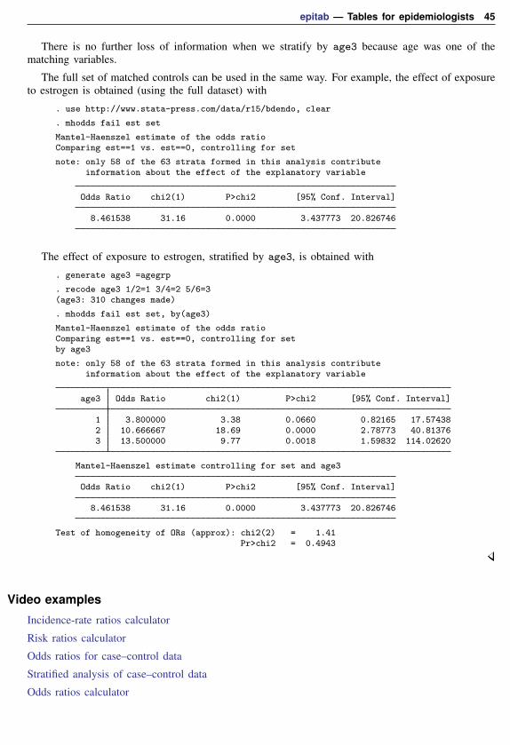
epitab — Tables for epidemiologists 45
There is no further loss of information when we stratify by age3 because age was one of thematching variables.
The full set of matched controls can be used in the same way. For example, the effect of exposureto estrogen is obtained (using the full dataset) with
. use http://www.stata-press.com/data/r15/bdendo, clear
. mhodds fail est set
Mantel-Haenszel estimate of the odds ratioComparing est==1 vs. est==0, controlling for set
note: only 58 of the 63 strata formed in this analysis contributeinformation about the effect of the explanatory variable
Odds Ratio chi2(1) P>chi2 [95% Conf. Interval]
8.461538 31.16 0.0000 3.437773 20.826746
The effect of exposure to estrogen, stratified by age3, is obtained with
. generate age3 =agegrp
. recode age3 1/2=1 3/4=2 5/6=3(age3: 310 changes made)
. mhodds fail est set, by(age3)
Mantel-Haenszel estimate of the odds ratioComparing est==1 vs. est==0, controlling for setby age3
note: only 58 of the 63 strata formed in this analysis contributeinformation about the effect of the explanatory variable
age3 Odds Ratio chi2(1) P>chi2 [95% Conf. Interval]
1 3.800000 3.38 0.0660 0.82165 17.574382 10.666667 18.69 0.0000 2.78773 40.813763 13.500000 9.77 0.0018 1.59832 114.02620
Mantel-Haenszel estimate controlling for set and age3
Odds Ratio chi2(1) P>chi2 [95% Conf. Interval]
8.461538 31.16 0.0000 3.437773 20.826746
Test of homogeneity of ORs (approx): chi2(2) = 1.41Pr>chi2 = 0.4943
Video examples
Incidence-rate ratios calculator
Risk ratios calculator
Odds ratios for case–control data
Stratified analysis of case–control data
Odds ratios calculator
46 epitab — Tables for epidemiologists
Glossary
attributable fraction. An attributable fraction is the reduction in the risk of a disease or othercondition of interest when a particular risk factor is removed.
case–control studies. In case–control studies, cases meeting a fixed criterion are matched to noncasesex post to study differences in possible covariates. Relative sample sizes are usually fixed at 1:1or 1:2 but sometimes vary once the survey is complete. In any case, sample sizes do not reflectthe distribution in the underlying population.
cohort studies. In cohort studies, a group that is well defined is monitored over time to track thetransition of noncases to cases. Cohort studies differ from incidence studies in that they can beretrospective as well as prospective.
confounding. In the analysis of contingency tables, factor or interaction effects are said to beconfounded when the effect of one factor is combined with that of another. For example, theeffect of alcohol consumption on esophageal cancer may be confounded with the effects of age,smoking, or both. In the presence of confounding, it is often useful to stratify on the confoundedfactors that are not of primary interest, in the above example, age and smoking.
cross-sectional or prevalence studies. Cross-sectional studies sample distributions of healthy anddiseased subjects in the population at one point in time.
crude estimate. A crude estimate has not been adjusted for the effects of other variables. Disregardinga stratification variable, for example, yields a crude estimate.
incidence and incidence rate. Incidence is the number of new failures (for example, number of newcases of a disease) that occur during a specified period in a population at risk (for example, of thedisease).
Incidence rate is incidence divided by the sum of the length of time each individual was exposedto the risk.
Do not confuse incidence with prevalence. Prevalence is the fraction of a population that has thedisease. Incidence refers to the rate at which people contract a disease, whereas prevalence is thetotal number actually sick at a given time.
incidence studies, longitudinal studies, and follow-up studies. Whichever word is used, these studiesmonitor a population for a time to track the transition of noncases into cases. Incidence studiesare prospective. Also see cohort studies.
matched case–control study. Also known as a retrospective study, a matched case–control study isa study in which persons with positive outcomes are each matched with one or more persons withnegative outcomes but with similar characteristics.
odds and odds ratio. The odds in favor of an event are o = p/(1 − p), where p is the probabilityof the event. Thus if p = 0.2, the odds are 0.25, and if p = 0.8, the odds are 4.
The log of the odds is ln(o) = logit(p) = ln{p/(1 − p)}, and logistic-regression models, forinstance, fit ln(o) as a linear function of the covariates.
The odds ratio is a ratio of two odds: o1/o0. The individual odds that appear in the ratio areusually for an experimental group and a control group, or two different demographic groups.
prevented fraction. A prevented fraction is the reduction in the risk of a disease or other conditionof interest caused by including a protective risk factor or public-health intervention.
prospective study. Also known as a prospective longitudinal study, a prospective study is a studybased on observations over the same subjects for a given period.
risk factor. This is a variable associated with an increased or decreased risk of failure.

epitab — Tables for epidemiologists 47
risk ratio. In a log-linear model, this is the ratio of probability of survival associated with aone-unit increase in a risk factor relative to that calculated without such an increase, that is,R(x + 1)/R(x). Given the exponential form of the model, R(x + 1)/R(x) is constant and isgiven by the exponentiated coefficient.
SMR. See standardized mortality (morbidity) ratio.
standardized mortality (morbidity) ratio. Standardized mortality (morbidity) ratio (SMR) is theobserved number of deaths divided by the expected number of deaths. It is calculated usingindirect standardization: you take the population of the group of interest—say, by age, sex, andother factors—and calculate the expected number of deaths in each cell (expected being definedas the number of deaths that would have been observed if those in the cell had the same mortalityas some other population). You then take the ratio to compare the observed with the expectednumber of deaths. For instance,
(1) (2) (1)×(2) (4)Population Deaths per 100,000 Expected # Observed
Age of group in general pop. of deaths deaths
25–34 95,965 105.2 100.9 9234–44 78,280 203.6 159.4 18044–54 52,393 428.9 224.7 24255–64 28,914 964.6 278.9 312Total 763.9 826
SMR = 826/763.9 = 1.08
stratified test. A stratified test is performed separately for each stratum. The stratum-specific resultsare then combined into an overall test statistic.
Stored resultsir and iri store the following in r():
Scalarsr(p) one-sided p-valuer(ird) incidence-rate differencer(lb ird) lower bound of CI for irdr(ub ird) upper bound of CI for irdr(irr) incidence-rate ratior(lb irr) lower bound of CI for irrr(ub irr) upper bound of CI for irrr(afe) attributable (prev.) fraction among exposedr(lb afe) lower bound of CI for afer(ub afe) upper bound of CI for afer(afp) attributable fraction for the populationr(crude) crude estimate (ir only)r(lb crude) lower bound of CI for cruder(ub crude) upper bound of CI for cruder(pooled) pooled estimate (ir only)r(lb pooled) lower bound of CI for pooledr(ub pooled) upper bound of CI for pooledr(chi2 mh) Mantel–Haenszel homogeneity χ2 (ir only)r(chi2 p) pooled homogeneity χ2
r(df) degrees of freedom (ir only)
48 epitab — Tables for epidemiologists
cs and csi store the following in r():
Scalarsr(p) two-sided p-valuer(rd) risk differencer(lb rd) lower bound of CI for rdr(ub rd) upper bound of CI for rdr(rr) risk ratior(lb rr) lower bound of CI for rrr(ub rr) upper bound of CI for rrr(or) odds ratior(lb or) lower bound of CI for orr(ub or) upper bound of CI for orr(afe) attributable (prev.) fraction among exposedr(lb afe) lower bound of CI for afer(ub afe) upper bound of CI for afer(afp) attributable fraction for the populationr(crude) crude estimate (cs only)r(lb crude) lower bound of CI for cruder(ub crude) upper bound of CI for cruder(pooled) pooled estimate (cs only)r(lb pooled) lower bound of CI for pooledr(ub pooled) upper bound of CI for pooledr(chi2 mh) Mantel–Haenszel heterogeneity χ2 (cs only)r(chi2 p) pooled heterogeneity χ2
r(df) degrees of freedom (cs only)r(chi2) χ2
r(p exact) 2-sided Fisher’s exact p (exact only)r(p1 exact) 1-sided Fisher’s exact p (exact only)
cc and cci store the following in r():
Scalarsr(p) two-sided p-valuer(p1 exact) one-sided p-value for Fisher’s exact testr(p exact) two-sided p-value for Fisher’s exact testr(or) odds ratior(lb or) lower bound of CI for orr(ub or) upper bound of CI for orr(afe) attributable (prev.) fraction among exposedr(lb afe) lower bound of CI for afer(ub afe) upper bound of CI for afer(afp) attributable fraction for the populationr(crude) crude estimate (cc only)r(lb crude) lower bound of CI for cruder(ub crude) upper bound of CI for cruder(pooled) pooled estimate (cc only)r(lb pooled) lower bound of CI for pooledr(ub pooled) upper bound of CI for pooledr(chi2 p) pooled heterogeneity χ2
r(chi2 bd) Breslow–Day χ2
r(df bd) degrees of freedom for Breslow–Day χ2
r(chi2 t) Tarone χ2
r(df t) degrees of freedom for Tarone χ2
r(df) degrees of freedomr(chi2) χ2

epitab — Tables for epidemiologists 49
tabodds stores the following in r():
Scalarsr(odds) oddsr(lb odds) lower bound for oddsr(ub odds) upper bound for oddsr(chi2 hom) χ2 test of homogeneityr(p hom) p-value for test of homogeneityr(df hom) degrees of freedom for χ2 test of homogeneityr(chi2 tr) χ2 for score test for trendr(p trend) p-value for score test for trend
mhodds stores the following in r():
Scalarsr(p) two-sided p-valuer(or) odds ratior(lb or) lower bound of CI for orr(ub or) upper bound of CI for orr(chi2 hom) χ2 test of homogeneityr(df hom) degrees of freedom for χ2 test of homogeneityr(chi2) χ2
mcc and mcci store the following in r():
Scalarsr(p exact) two-sided p-value for McNemar’s testr(or) odds ratior(lb or) lower bound of CI for orr(ub or) upper bound of CI for orr(D f) difference in proportion with factorr(lb D f) lower bound of CI for D fr(ub D f) upper bound of CI for D fr(R f) ratio of proportion with factorr(lb R f) lower bound of CI for R fr(ub R f) upper bound of CI for R fr(RD f) relative difference in proportion with factorr(lb RD f) lower bound of CI for RD fr(ub RD f) upper bound of CI for RD fr(chi2) χ2
Methods and formulasThe notation for incidence-rate data is
Exposed Unexposed Total
Cases a b M1
Person-time N1 N0 T
The notation for 2× 2 tables is
Exposed Unexposed Total
Cases a b M1
Controls c d M0
Total N1 N0 T

50 epitab — Tables for epidemiologists
The notation for 2× k tables is
Exposure level1 2 . . . k Total
Cases a1 a2 . . . ak M1
Controls c1 c2 . . . ck M0
Total N1 N2 . . . Nk T
If the tables are stratified, all quantities are indexed by i, the stratum number.
We will refer to Fleiss, Levin, and Paik (2003); Kleinbaum, Kupper, and Morgenstern (1982); andRothman (1986) so often that we will adopt the notation F-23 to mean Fleiss, Levin, and Paik (2003)page 23; KKM-52 to mean Kleinbaum, Kupper, and Morgenstern (1982) page 52; and R-164 to meanRothman (1986) page 164.
We usually avoid making the continuity corrections to χ2 statistics, following the advice ofKKM-292: “. . . the use of a continuity correction has been the subject of considerable debate in thestatistical literature . . . . On the basis of our evaluation of this debate and other evidence, we donot recommend the use of the continuity correction.” Breslow and Day (1980, 133), on the otherhand, argue for inclusion of the correction, but not strongly. Their summary is that for small datasets,one should use exact statistics. In practice, we believe that the adjustment makes little difference forreasonably sized datasets.
Methods and formulas are presented under the following headings:
Unstratified incidence-rate data (ir and iri)Unstratified cumulative incidence data (cs and csi)Unstratified case–control data (cc and cci)Unstratified matched case–control data (mcc and mcci)Stratified incidence-rate data (ir with the by() option)Stratified cumulative incidence data (cs with the by() option)Stratified case–control data (cc with by() option, mhodds, tabodds)
Unstratified incidence-rate data (ir and iri)
The incidence-rate difference is defined as Id = a/N1 − b/N0 (R-164). The standard error of thedifference is sId ≈
√a/N2
1 + b/N20 (R-170), from which confidence intervals are calculated.
The incidence-rate ratio is defined as Ir = (a/N1)/(b/N0) (R-164). Let pl and pu be the exactconfidence interval of the binomial probability for observing a successes in M1 trials (obtainedfrom cii proportions; see [R] ci). The exact confidence interval for the incidence ratio is then(plN0)/{(1− pl)N1} to (puN0)/{(1− pu)N1} (R-166).
The attributable fraction among the exposed is defined as AFE = (Ir−1)/Ir for Ir ≥ 1 (KKM-164;R-38); the confidence interval is obtained by similarly transforming the interval values of Ir. Theattributable fraction for the population is AF = AFE · a/M1 (KKM-161); no confidence interval isreported. For Ir < 1, the prevented fraction among the exposed is defined as PFE = 1−Ir (KKM-166;R-39); the confidence interval is obtained by similarly transforming the interval values of Ir. Theprevented fraction for the population is PF = PFE·N1/T (KKM-165); no confidence interval is reported.
The “midp” one-sided exact significance (R-155) is calculated as the binomial probability (withn = M1 and p = N1/T ) Pr(k = a)/2 + Pr(k > a) if Ir ≥ 1 and Pr(k = a)/2 + Pr(k < a)otherwise. The two-sided significance is twice the one-sided significance (R-155). If preferred, youcan obtain nonmidp exact probabilities (and, to some ways of thinking, a more reasonable definitionof two-sided significance) using bitest; see [R] bitest.

epitab — Tables for epidemiologists 51
Unstratified cumulative incidence data (cs and csi)
The risk difference is defined as Rd = a/N1 − b/N0 (R-164). Its standard error is
sRd≈{ac
N31
+bd
N30
}1/2
(R-172), from which confidence intervals are calculated.
The risk ratio is defined as Rr = (a/N1)/(b/N0) (R-165). The standard error of lnRr is
s lnRr≈(
c
aN1+
d
bN0
)1/2
(R-173), from which confidence intervals are calculated.
For Rr ≥ 1, the attributable fraction among the exposed is calculated as AFE = (Rr − 1)/Rr(KKM-164; R-38); the confidence interval is obtained by similarly transforming the interval values forRr. The attributable fraction for the population is calculated as AF = AFE · a/M1 (KKM-161); noconfidence interval is reported, but F-128 provides
{c+ (a+ d)AF
bT
}1/2
as the approximate standard error of ln(1− AF).
For Rr < 1, the prevented fraction among the exposed is calculated as PFE = 1−Rr (KKM-166;R-39); the confidence interval is obtained by similarly transforming the interval values for Rr. Theprevented fraction for the population is calculated as PF = PFE · N1/T ; no confidence interval isreported.
The odds ratio, available with the or option, is defined as ψ = (ad)/(bc) (R-165). Severalconfidence intervals are available. The default interval for cs and csi is the Cornfield (1956)approximate interval. If we let zα be the index from a normal distribution for an α significance level,the Cornfield interval (ψl, ψu) is calculated from
ψl = al(M0 −N1 + al)/{
(N1 − al)(M1 − al)}
ψu = au(M0 −N1 + au)/{
(N1 − au)(M1 − au)}
where au and al are determined iteratively from
ai+1 = a± zα(
1
ai+
1
N1 − ai+
1
M1 − ai+
1
M0 −N1 + ai
)−1/2
(Newman 2001, sec. 4.4). ai+1 converges to au using the plus sign and al using the minus sign. a0 istaken as a. With small numbers, the iterative technique may fail. It is then restarted by decrementing(al) or incrementing (au) a0. If that fails, a0 is again decremented or incremented and iterationsrestarted, and so on, until a terminal condition is met (a0 < 0 or a0 > M1), at which point the valueis not calculated.

52 epitab — Tables for epidemiologists
The Woolf odds-ratio confidence intervals are available with cs and csi. The Woolf method(Woolf 1955; R-173; Schlesselman 1982, 176), available with the woolf option, estimates thestandard error of lnψ by
s lnψ =
(1
a+
1
b+
1
c+
1
d
)1/2
from which confidence intervals are calculated. The Woolf interval cannot be calculated when thereexists a zero cell. Sometimes the Woolf interval is called the “logit interval” (Breslow and Day 1980,134).
The χ2 statistic, reported by default, can be calculated as
χ2 =(ad− bc)2TM1M0N1N0
(Schlesselman 1982, 179).
Fisher’s exact test, available with the exact option, is calculated as described in [R] tabulatetwoway.
Unstratified case–control data (cc and cci)
cc and cci report by default the same odds ratio, ψ, that is available with the or option in cs andcsi. But cc and cci calculate the confidence interval differently: they default to the exact odds-ratiointerval, not the Cornfield interval, but you can request the Cornfield interval with the cornfieldoption. The 1− α exact interval (R,R) is calculated from
α/2 =
∑min(N1,M1)k=a
(N1
k
)(N0
M1−k)Rk∑min(N1,M1)
k=max(0,M1−N0)
(N1
k
)(N0
M1−k)Rk
and
1− α/2 =
∑min(N1,M1)k=a+1
(N1
k
)(N0
M1−k)Rk∑min(N1,M1)
k=max(0,M1−N0)
(N1
k
)(N0
M1−k)Rk
(R-169). The equations invert two one-sided Fisher exact tests.
cc and cci also report the same tests of significance as cs and csi: the χ2 statistic is the default,and Fisher’s exact test is obtained with the exact option. The odds ratio, ψ, is used as an estimateof the risk ratio in calculating attributable or prevented fractions. For ψ ≥ 1, the attributable fractionamong the exposed is calculated as AFE = (ψ− 1)/ψ (KKM-164); the confidence interval is obtainedby similarly transforming the interval values for ψ. The attributable fraction for the population iscalculated as AF = AFE · a/M1 (KKM-161). No confidence interval is reported; however, F-152provides (
a
M1b+
c
M0d
)1/2
as the standard error of ln(1− AF).
For ψ < 1, the prevented fraction among the exposed is calculated as PFE = 1 − ψ (KKM-166);the confidence interval is obtained by similarly transforming the interval values for ψ. The preventedfraction for the population is calculated as PF = {(a/M1)PFE}/{(a/M1)PFE + ψ} (KKM-165); noconfidence interval is reported.

epitab — Tables for epidemiologists 53
Unstratified matched case–control data (mcc and mcci)
Referring to the table at the beginning of Methods and formulas, the columns of the 2× 2 tableindicate controls; the rows are cases. Each entry in the table reflects a pair of a matched case andcontrol.
McNemar’s (1947) χ2 is defined as
χ2 =(b− c)2
b+ c
(KKM-389).
The proportion of controls with the factor is p1 = N1/T , and the proportion of cases with thefactor is p2 =M1/T .
The difference in the proportions is Pd = p2− p1. An estimate of its standard error when the twounderlying proportions are not hypothesized to be equal is
sPd≈ {(a+ d)(b+ c) + 4bc}1/2
T 3/2
(F-378), from which confidence intervals are calculated. The confidence interval uses a continuitycorrection (F-378, eq. 13.15).
The ratio of the proportions is Pr = p2/p1 (R-276, R-278). The standard error of lnPr is
s lnPr≈(b+ c
M1N1
)1/2
(R-276), from which confidence intervals are calculated.
The relative difference in the proportions is Pe = (b− c)/(b+ d) (F-379). Its standard error is
sPe≈ (b+ d)−2 {(b+ c+ d)(bc+ bd+ cd)− bcd}1/2
(F-379), from which confidence intervals are calculated.
The odds ratio is ψ = b/c (F-376), and the exact Fisher confidence interval is obtained bytransforming into odds ratios the exact binomial confidence interval for the binomial parameter fromobserving b successes in b + c trials (R-264). Binomial confidence limits are obtained from ciiproportions (see [R] ci) and are transformed by p/(1− p).
The exact McNemar significance probability is a two-tailed exact test of H0 : ψ = 1. The p-value,calculated from the binomial distribution, is
min
1, 2
min(b,c)∑k=0
(b+ c
k
)(1
2
)b+c(Agresti 2013, 416).� �
Quinn McNemar (1900–1986) was born in West Virginia and attended college there and inPennsylvania. After a brief spell of high school teaching, he began graduate study of psychologyat Stanford and then joined the faculty. McNemar’s text Psychological Statistics, first publishedin 1949, was widely influential, and he made many substantive and methodological contributionsto the application of statistics in psychology.� �

54 epitab — Tables for epidemiologists
Stratified incidence-rate data (ir with the by() option)
Statistics presented for each stratum are calculated independently according to the formulas inUnstratified incidence-rate data (ir and iri) above. Within strata, the Mantel–Haenszel style weight isWi = biN1i/Ti, and the Mantel–Haenszel combined incidence-rate ratio (Rothman and Boice 1982)is
Imh =
∑i aiN0i/Ti∑
iWi
(R-196). The standard error for the log of the incidence-rate ratio was derived by Greenland andRobins (1985, 63) and appears in R-213:
s lnImh≈
{ ∑iM1iN1iN0i/T
2i(∑
i aiN0i/Ti)(∑
i biN1i/Ti)}1/2
The confidence interval is calculated first on the log scale and then is transformed.
For standardized rates, let wi be the user-specified weight within stratum i. The standardized ratedifference (the ird option) and rate ratio are defined as
SRD =
∑i wi(R1i −R0i)∑
i wi
SRR =
∑i wiR1i∑i wiR0i
(R-229). The standard error of SRD is
sSRD ≈
{1
(∑i wi)
2
∑i
w2i
(aiN2
1i
+biN2
0i
)}1/2
(R-231), from which confidence intervals are calculated. The standard error of ln(SRR) is
s ln(SRR) ≈{∑
i w2i ai/N
21i
(∑i wiR1i)2
+
∑i w
2i bi/N
20i
(∑i wiR0i)2
}1/2
(R-231), from which confidence intervals are calculated.
Internally and externally standardized measures are calculated using wi = N1i and wi = N0i,respectively, and are obtained with the istandard and estandard options, respectively.
Directly pooled estimates are available with the pool option. The directly pooled estimate is aweighted average of stratum-specific estimates; each weight, wi, is inversely proportional to thevariance of the estimate for stratum i. The variances for rate differences come from the formulas inUnstratified incidence-rate data (ir and iri), while the variances of log rate-ratios are estimated by(1/ai+1/bi) (R-184). Ratios are averaged in the log scale before being exponentiated. The standarderror of the directly pooled estimate is calculated as 1/
√∑wi, from which confidence intervals are
calculated (R-183–185); the calculation for ratios again uses the log scale.
For rate differences, the χ2 test of homogeneity is calculated as∑
(Rdi− Rd)2/var(Rdi), whereRdi are the stratum-specific rate differences and Rd is the directly pooled estimate. The number ofdegrees of freedom is one less than the number of strata (R-222).
For rate ratios, the same calculation is made, except that it is made on a logarithmic scaleusing ln(Rri) (R-222), and ln(Rd) may be the log of either the directly pooled estimate or theMantel–Haenszel estimate.

epitab — Tables for epidemiologists 55
Stratified cumulative incidence data (cs with the by() option)
Statistics presented for each stratum are calculated independently according to the formulas inUnstratified cumulative incidence data (cs and csi) above. The Mantel–Haenszel χ2 test (Mantel andHaenszel 1959) is
χ2mh =
{∑i(ai −N1iM1i/Ti)
}2∑i(N1iN0iM1iM0i)/
{T 2i (Ti − 1)
}(R-206).
For the odds ratio (available with the or option), the Mantel–Haenszel weight is Wi = bici/Ti,and the combined odds ratio (Mantel and Haenszel 1959) is
ψmh =
∑i aidi/Ti∑iWi
(R-195). The standard error (Robins, Breslow, and Greenland 1986) is
s lnψmh≈
{ ∑i PiRi
2(∑
iRi)2 +
∑i PiSi +QiRi
2∑iRi
∑i Si
+
∑iQiSi
2(∑
i Si)2}1/2
wherePi = (ai + di)/Ti
Qi = (bi + ci)/Ti
Ri = aidi/Ti
Si = bici/Ti
(R-220).
For the risk ratio (the default), the Mantel–Haenszel-style weight is Wi = biN1i/Ti, and thecombined risk ratio (Rothman and Boice 1982) is
Rmh =
∑i aiN0i/Ti∑
iWi
(R-196). The standard error (Greenland and Robins 1985) is
s lnRmh≈
{∑i(M1iN1iN0i − aibiTi)/T 2
i(∑i aiN0i/Ti
)(∑i biN1i/Ti
)}1/2
(R-216), from which confidence intervals are calculated.
For standardized rates, let wi be the user-specified weight within stratum i. The standardizedrate difference (SRD, the rd option) and rate ratios (SRR, the default) are defined as in Stratifiedincidence-rate data (ir with the by() option), where the individual risks are defined R1i = ai/N1i
and R0i = bi/N0i. The standard error of SRD is
sSRD ≈
[1
(∑i wi)
2
∑i
w2i
{ai(N1i − ai)
N31i
+bi(N0i − bi)
N30i
}]1/2
56 epitab — Tables for epidemiologists
(R-231), from which confidence intervals are calculated. The standard error of ln(SRR) is
s ln(SRR) ≈{∑
i w2i ai(N1i − ai)/N3
1i
(∑i wiR1i)2
+
∑i w
2i bi(N0i − bi)/N3
0i
(∑i wiR0i)2
}1/2
(R-231), from which confidence intervals are calculated.
Internally and externally standardized measures are calculated using wi = N1i and wi = N0i,respectively, and are obtained with the istandard and estandard options, respectively.
Directly pooled estimates of the odds ratio are available when you specify both the pool and oroptions. The directly pooled estimate is a weighted average of stratum-specific log odds-ratios; eachweight, wi, is inversely proportional to the variance of the log odds-ratio for stratum i. The variancesof the log odds-ratios are estimated by Woolf’s method, described under Unstratified cumulativeincidence data (cs and csi). The standard error of the directly pooled log odds-ratio is calculatedas 1/
√∑wi, from which confidence intervals are calculated and then exponentiated (Kahn and
Sempos 1989, 113–115).
Direct pooling is also available for risk ratios and risk differences; the variance formulas may befound in Unstratified cumulative incidence data (cs and csi). The directly pooled risk ratio is providedwhen the pool option is specified. The directly pooled risk difference is provided only when youspecify the pool and rd options, and one of the estandard, istandard, and standard() options.
For risk differences, the χ2 test of homogeneity is calculated as∑
(Rdi− Rd)2/var(Rdi), whereRdi are the stratum-specific risk differences and Rd is the directly pooled estimate. The number ofdegrees of freedom is one less than the number of strata (R-222).
For risk and odds ratios, the same calculation is made, except that it is made in the log scale usingln(Rri) or ln(ψi) (R-222), and ln(Rd) may be the log of either the directly pooled estimate or theMantel–Haenszel estimate.
Stratified case–control data (cc with by() option, mhodds, tabodds)
Statistics presented for each stratum are calculated independently according to the formulas inUnstratified cumulative incidence data (cs and csi) above. The combined odds ratio, ψmh, and thetest that ψmh = 1 (χ2
mh) are calculated as described in Stratified cumulative incidence data (cs withthe by() option) above.
For standardized weights, let wi be the user-specified weight within stratum i. The standardizedodds ratio (the standard() option) is calculated as
SOR =
∑i wiai/ci∑i wibi/di
(Greenland 1986, 473). The standard error of ln(SOR) is
s ln(SOR) =
{∑i(wiai/ci)
2( 1ai
+ 1bi
+ 1ci
+ 1di)(∑
i wiai/ci)2
}1/2
from which confidence intervals are calculated. The internally and externally standardized odds ratiosare calculated using wi = ci and wi = di, respectively.

epitab — Tables for epidemiologists 57
The directly pooled estimate of the odds ratio (the pool option) is calculated as described inStratified cumulative incidence data (cs with the by() option) above.
The directly pooled and Mantel–Haenszel χ2 tests of homogeneity are calculated as∑{
ln(Rri)−ln(Rr)
}2/var
{ln(Rri)
}, where Rri are the stratum-specific odds ratios and Rr is the pooled estimate
(Mantel–Haenszel or directly pooled). The number of degrees of freedom is one less than the numberof strata (R-222).
The Breslow–Day χ2 test of homogeneity is available with the bd option. Let ψ be the Mantel–Haenszel estimate of the common odds ratio, and let Ai(ψ) be the fitted count for cell a; Ai(ψ) isfound by solving the quadratic equation
A(M0 −N1 +A) = (ψ)(M1 −A)(N1 −A)
and choosing the root that makes all cells in stratum i positive. Let Var(ai; ψ) be the estimatedvariance of ai conditioned on the margins and on an odds ratio of ψ:
Var(ai; ψ) =
{1
Ai(ψ)+
1
M1i −Ai(ψ)+
1
N1i −Ai(ψ)+
1
M0i −N1i +Ai(ψ)
}−1
The Breslow–Day χ2 statistic is then ∑i
{ai −Ai(ψ)}2
Var(ai; ψ)
The Tarone χ2 test of homogeneity (the tarone option) is calculated as∑i
{ai −Ai(ψ)}2
Var(ai; ψ)−{∑i ai −
∑iAi(ψ)}2∑
iVar(ai; ψ)
Tarone (1985) provides this correction to the Breslow–Day statistic to ensure that its distributionis asymptotically chi-squared. Without the correction, the Breslow–Day statistic does not necessarilyfollow a chi-squared distribution because it is based on the Mantel–Haenszel estimate, ψ, which isan inefficient estimator of the common odds ratio.
When the exposure variable has multiple levels, mhodds calculates an approximate estimate ofthe log odds-ratio for a one-unit increase in exposure as the ratio of the score statistic, U , to itsvariance, V (Clayton and Hills 1993, 103), which are defined below. This is a one-step Newton-Raphson approximation to the maximum likelihood estimate. Within-stratum estimates are combinedwith Mantel–Haenszel weights.
By default, both tabodds and mhodds produce test statistics and confidence intervals based onscore statistics (Clayton and Hills 1993). tabodds reports confidence intervals for the odds of theith exposure level, unless the adjust() or or option is specified. The confidence interval for oddsi,i = 1, . . . , k, is given by
oddsi · exp(±z√1/ai + 1/ci
)The score χ2 test of homogeneity of odds is calculated as
χ2k−1 =
T (T − 1)
M1M0
k∑i=1
(ai − Ei)2
Ni
where Ei = (M1Ni)/T .

58 epitab — Tables for epidemiologists
Let li denote the value of the exposure at the ith level. The score χ2 test for trend of odds iscalculated as
χ21 =
U2
V
where
U =M1M0
T
( k∑i=1
ailiM1−
k∑i=1
ciliM0
)and
V =M1M0
T
{∑ki=1Nil
2i − (
∑ki=1Nili)
2/T
T − 1
}
AcknowledgmentsWe thank Hal Morgenstern of the Department of Epidemiology at the University of Michigan,
Ardythe Morrow of the Cincinnati Children’s Hospital, and the late Stewart West of Baylor Collegeof Medicine for their assistance in designing these commands.
We thank the late Jonathan Freeman at the Department of Epidemiology at Harvard School ofPublic Health for encouraging us to extend these commands to include tests for homogeneity, forhelpful comments on the default behavior of the commands, and for his comments on an early draftof this section.
We thank David Clayton (retired) of the Cambridge Institute for Medical Research and MichaelHills (retired) of the London School of Hygiene and Tropical Medicine, who wrote the originalversions of mhodds and tabodds.
Finally, we thank William Dupont and Dale Plummer, both at the Department of Biostatistics,Vanderbilt University, for their contribution to the implementation of exact confidence intervals forthe odds ratios for cc and cci.
epitab — Tables for epidemiologists 59� �John Snow (1813–1858) was born in York, England. From age 14, he worked as an apprenticeand assistant to surgeons in northeast England and Yorkshire. In 1836, Snow moved to London;he was admitted to the Royal College of Surgeons in 1838 and the Royal College of Physiciansin 1850. He made outstanding contributions to the adoption of anesthesia and is considered oneof the originators of modern epidemiology. Snow died following a stroke in 1858.
Snow calculated dosages for ether and chloroform. He personally administered chloroform toQueen Victoria for the births of her last two children, which helped obstetric anesthesia gainwider acceptance.
Snow was skeptical of the miasma theory that cholera was caused by foul air. His essay Onthe Mode of Communication of Cholera was first published in 1849 and then greatly enlargedin 1855 with the results of his very detailed investigation of the role of water supply in theepidemic of 1854 in the Soho district of London. Snow identified the source of the outbreakas the public water pump on Broad Street (now Broadwick Street), leading the local council toremove the pump handle. It was later discovered that the well had been dug very close to an oldcesspit. He also mapped the clustering of cholera cases around the pump and related mortalityto water sources, clearly showing higher death rates in areas supplied by the Southwark andVauxhall Waterworks Company, which was taking water from sewage-polluted sections of theRiver Thames. Snow is widely regarded as a pioneer in public health, epidemiology, and medicalgeography.� �
� �Janet Elizabeth Lane-Claypon (1877–1967) was a pioneer in the use of cohort and case–controlstudies. She was born in Lincolnshire county, England, and began her studies at the LondonSchool of Medicine for Women in 1898. From 1907 to 1912, she was at the Lister Institute ofPreventive Medicine, where she was a colleague of Major Greenwood. By the end of her studies,she had obtained a doctorate in both physiology and medicine.
In 1912, Lane-Claypon published one of the first retrospective cohort studies, examining theweight gain of babies fed cow’s milk versus babies fed breast milk. Using statistical techniques,she determined that babies fed breast milk gained weight faster; she later employed that knowledgeto become a public health advocate for breast feeding.
She also conducted one of the first case–control studies, examining risk factors associated withbreast cancer. Her study included 500 women without breast cancer and 500 women with breastcancer. To obtain what was at the time a remarkably large sample, she coordinated data collectionfrom nine different hospitals. Carefully controlling for variables including occupation and infantmortality, she determined that factors like age at first pregnancy, age at menopause, and numberof children all influence the incidence of breast cancer; these factors are still considered to beamong the prime determinants.
In conjunction with the Ministry of Health, in 1926 Lane-Claypon published one of the firststudies to contain long-term follow-up results. In that study, she followed patients who hadundergone surgery for breast cancer for up to 10 years after the operation. As is still the casetoday, her study showed that the sooner the cancer was treated, the better the woman’s chancefor long-term survival. Notably, her study was also among the first to consider survivorship bias.� �
60 epitab — Tables for epidemiologists
ReferencesAgresti, A. 1999. On logit confidence intervals for the odds ratio with small samples. Biometrics 55: 597–602.
. 2013. Categorical Data Analysis. 3rd ed. Hoboken, NJ: Wiley.
Boice, J. D., Jr., and R. R. Monson. 1977. Breast cancer in women after repeated fluoroscopic examinations of thechest. Journal of the National Cancer Institute 59: 823–832.
Breslow, N. E. 1996. Statistics in epidemiology: The case–control study. Journal of the American Statistical Association91: 14–28.
Breslow, N. E., and N. E. Day. 1980. Statistical Methods in Cancer Research: Vol. 1—The Analysis of Case–ControlStudies. Lyon: IARC.
Brown, C. C. 1981. The validity of approximation methods for interval estimation of the odds ratio. American Journalof Epidemiology 113: 474–480.
Carlin, J. B., and S. Vidmar. 2000. sbe35: Menus for epidemiological statistics. Stata Technical Bulletin 56: 15–16.Reprinted in Stata Technical Bulletin Reprints, vol. 10, pp. 86–87. College Station, TX: Stata Press.
Clayton, D. G., and M. Hills. 1993. Statistical Models in Epidemiology. Oxford: Oxford University Press.
. 1995. ssa8: Analysis of case-control and prevalence studies. Stata Technical Bulletin 27: 26–31. Reprinted inStata Technical Bulletin Reprints, vol. 5, pp. 227–233. College Station, TX: Stata Press.
Cornfield, J. 1956. A statistical problem arising from retrospective studies. In Vol. 4 of Proceedings of the ThirdBerkeley Symposium, ed. J. Neyman, 135–148. Berkeley, CA: University of California Press.
Cummings, P. 2009. Methods for estimating adjusted risk ratios. Stata Journal 9: 175–196.
Dohoo, I., W. Martin, and H. Stryhn. 2010. Veterinary Epidemiologic Research. 2nd ed. Charlottetown, Prince EdwardIsland: VER Inc.
. 2012. Methods in Epidemiologic Research. Charlottetown, Prince Edward Island: VER Inc.
Doll, R., and A. B. Hill. 1966. Mortality of British doctors in relation to smoking: Observations on coronarythrombosis. Journal of the National Cancer Institute, Monographs 19: 205–268.
Dupont, W. D. 2009. Statistical Modeling for Biomedical Researchers: A Simple Introduction to the Analysis ofComplex Data. 2nd ed. Cambridge: Cambridge University Press.
Dupont, W. D., and W. D. Plummer, Jr. 1999. sbe31: Exact confidence intervals for odds ratios from case–controlstudies. Stata Technical Bulletin 52: 12–16. Reprinted in Stata Technical Bulletin Reprints, vol. 9, pp. 150–154.College Station, TX: Stata Press.
Fagerland, M. W. 2012. Exact and mid-p confidence intervals for the odds ratio. Stata Journal 12: 505–514.
Fleiss, J. L., B. Levin, and M. C. Paik. 2003. Statistical Methods for Rates and Proportions. 3rd ed. New York:Wiley.
Gart, J. J., and D. G. Thomas. 1982. The performance of three approximate confidence limit methods for the oddsratio. American Journal of Epidemiology 115: 453–470.
Gini, R., and J. Pasquini. 2006. Automatic generation of documents. Stata Journal 6: 22–39.
Glass, R. I., A. M. Svennerholm, B. J. Stoll, M. R. Khan, K. M. Hossain, M. I. Huq, and J. Holmgren. 1983.Protection against cholera in breast-fed children by antibodies in breast milk. New England Journal of Medicine308: 1389–1392.
Gleason, J. R. 1999. sbe30: Improved confidence intervals for odds ratios. Stata Technical Bulletin 51: 24–27.Reprinted in Stata Technical Bulletin Reprints, vol. 9, pp. 146–150. College Station, TX: Stata Press.
Greenhouse, S. W., and J. B. Greenhouse. 1998. Cornfield, Jerome. In Vol. 1 of Encyclopedia of Biostatistics, ed.P. Armitage and T. Colton, 955–959. Chichester, UK: Wiley.
Greenland, S. 1986. Estimating variances of standardized estimators in case–control studies and sparse data. Journalof Chronic Diseases 39: 473–477.
Greenland, S., ed. 1987. Evolution of Epidemiologic Ideas: Annotated Readings on Concepts and Methods. NewtonLower Falls, MA: Epidemiology Resources.
Greenland, S., and J. M. Robins. 1985. Estimation of a common effect parameter from sparse follow-up data.Biometrics 41: 55–68.

epitab — Tables for epidemiologists 61
. 1988. Conceptual problems in the definition and interpretation of attributable fractions. American Journal ofEpidemiology 128: 1185–1197.
Haldane, J. B. S. 1957. Graphical methods in enzyme chemistry. Nature 179: 832.
Hastorf, A. H., E. R. Hilgard, and R. R. Sears. 1988. Quinn McNemar (1900–1986). American Psychologist 43:196–197.
Hempel, S. 2006. The Medical Detective: John Snow, Cholera and the Mystery of the Broad Street Pump. London:Granta Books.
Hill, W. G. 1984. Barnet Woolf. Year Book, Royal Society of Edinburgh 1984 214–219.
Jewell, N. P. 2004. Statistics for Epidemiology. Boca Raton, FL: Chapman & Hall/CRC.
Jick, H., O. S. Miettinen, R. K. Neff, S. Shapiro, O. P. Heinonen, and D. Slone. 1973. Coffee and myocardialinfarction. New England Journal of Medicine 289: 63–67.
Johnson, S. 2006. The Ghost Map: The Story of London’s Most Terrifying Epidemic—and How It Changed Science,Cities, and the Modern World. London: Penguin Books.
Kahn, H. A., and C. T. Sempos. 1989. Statistical Methods in Epidemiology. New York: Oxford University Press.
Kleinbaum, D. G., L. L. Kupper, and H. Morgenstern. 1982. Epidemiologic Research: Principles and QuantitativeMethods (Industrial Health and Safety). New York: Wiley.
Lilienfeld, D. E., and P. D. Stolley. 1994. Foundations of Epidemiology. 3rd ed. New York: Oxford University Press.
Lopez-Vizcaıno, M. E., M. I. Perez-Santiago, and L. Abraira-Garcıa. 2000a. sbe32.1: Automated outbreak detectionfrom public health surveillance data: Errata. Stata Technical Bulletin Reprints 55: 2.
. 2000b. sbe32: Automated outbreak detection from public health surveillance data. Stata Technical Bulletin 54:23–25. Reprinted in Stata Technical Bulletin Reprints, vol. 9, pp. 154–157. College Station, TX: Stata Press.
MacMahon, B., S. Yen, D. Trichopoulos, K. Warren, and G. Nardi. 1981. Coffee and cancer of the pancreas. NewEngland Journal of Medicine 304: 630–633.
Mantel, N., and W. Haenszel. 1959. Statistical aspects of the analysis of data from retrospective studies of disease.Journal of the National Cancer Institute 22: 719–748. Reprinted in Evolution of Epidemiologic Ideas: AnnotatedReadings on Concepts and Methods, ed. S. Greenland, pp. 112–141. Newton Lower Falls, MA: EpidemiologyResources.
Markel, H. 2013. Happy birthday, Dr Snow. Journal of the American Medical Association 309: 995–996.
McNemar, Q. 1947. Note on the sampling error of the difference between correlated proportions or percentages.Psychometrika 12: 153–157.
Newman, S. C. 2001. Biostatistical Methods in Epidemiology. New York: Wiley.
Orsini, N., R. Bellocco, M. Bottai, A. Wolk, and S. Greenland. 2008. A tool for deterministic and probabilisticsensitivity analysis of epidemiologic studies. Stata Journal 8: 29–48.
Pearce, M. S., and R. Feltbower. 2000. stburlstb56.pdfsg149: Tests for seasonal data via the Edwards and Walter& Elwood tests. Stata Technical Bulletin 56: 47–49. Reprinted in Stata Technical Bulletin Reprints, vol. 10, pp.214–217. College Station, TX: Stata Press.
Reilly, M., and A. Salim. 2000. sxd2: Computing optimal sampling designs for two-stage studies. Stata TechnicalBulletin 58: 37–41. Reprinted in Stata Technical Bulletin Reprints, vol. 10, pp. 376–382. College Station, TX:Stata Press.
Robins, J. M., N. E. Breslow, and S. Greenland. 1986. Estimators of the Mantel–Haenszel variance consistent in bothsparse data and large-strata limiting models. Biometrics 42: 311–323.
Rothman, K. J. 1982. Spermicide use and Down’s syndrome. American Journal of Public Health 72: 399–401.
. 1986. Modern Epidemiology. Boston: Little, Brown.
. 2012. Epidemiology: An Introduction. 2nd ed. New York: Oxford University Press.
Rothman, K. J., and J. D. Boice, Jr. 1982. Epidemiologic Analysis with a Programmable Calculator. Brookline, MA:Epidemiology Resources.
Rothman, K. J., D. C. Fyler, A. Goldblatt, and M. B. Kreidberg. 1979. Exogenous hormones and other drug exposuresof children with congenital heart disease. American Journal of Epidemiology 109: 433–439.

62 epitab — Tables for epidemiologists
Rothman, K. J., S. Greenland, and T. L. Lash. 2008. Modern Epidemiology. 3rd ed. Philadelphia: Lippincott Williams& Wilkins.
Rothman, K. J., and R. R. Monson. 1973. Survival in trigeminal neuralgia. Journal of Chronic Diseases 26: 303–309.
Royston, P., and A. G. Babiker. 2002. A menu-driven facility for complex sample size calculation in randomizedcontrolled trials with a survival or a binary outcome. Stata Journal 2: 151–163.
Schlesselman, J. J. 1982. Case–Control Studies: Design, Conduct, Analysis. New York: Oxford University Press.
Selvin, S. 2011. Statistical Tools for Epidemiologic Research. New York: Oxford University Press.
Snow, J. 1855. On the Mode of Communication of Cholera. 2nd ed. London: Churchill.
Tarone, R. E. 1985. On heterogeneity tests based on efficient scores. Biometrika 72: 91–95.
University Group Diabetes Program. 1970. A study of the effects of hypoglycemic agents on vascular complicationsin patients with adult-onset diabetes, II: Mortality results. Diabetes 19, supplement 2: 789–830.
Vinten-Johansen, P., H. Brody, N. Paneth, S. Rachman, and M. Rip. 2003. Cholera, Chloroform, and the Science ofMedicine: A Life of John Snow. New York: Oxford University Press.
Walker, A. M. 1991. Observation and Inference: An Introduction to the Methods of Epidemiology. Newton LowerFalls, MA: Epidemiology Resources.
Wang, Z. 1999. sbe27: Assessing confounding effects in epidemiological studies. Stata Technical Bulletin 49: 12–15.Reprinted in Stata Technical Bulletin Reprints, vol. 9, pp. 134–138. College Station, TX: Stata Press.
. 2007. Two postestimation commands for assessing confounding effects in epidemiological studies. Stata Journal7: 183–196.
Woodward, M. 2014. Epidemiology: Study Design and Data Analysis. 3rd ed. Boca Raton, FL: Chapman & Hall/CRC.
Woolf, B. 1955. On estimating the relation between blood group disease. Annals of Human Genetics 19: 251–253.Reprinted in Evolution of Epidemiologic Ideas: Annotated Readings on Concepts and Methods, ed. S. Greenland,pp. 108–110. Newton Lower Falls, MA: Epidemiology Resources.
Also see[ST] stcox — Cox proportional hazards model
[R] bitest — Binomial probability test
[R] ci — Confidence intervals for means, proportions, and variances
[R] clogit — Conditional (fixed-effects) logistic regression
[R] dstdize — Direct and indirect standardization
[R] logistic — Logistic regression, reporting odds ratios
[R] poisson — Poisson regression
[R] symmetry — Symmetry and marginal homogeneity tests
[R] tabulate twoway — Two-way table of frequencies