tm cloud,.--., ozone ata · 37 june 8 821 47s 26e 47s 26e 46s 25e 38 june 8 825 45s 79w 45s 79w 44s...
TRANSCRIPT
.- · .~., . .- ,. .. ;/ . . -. , , ~, ~ . I .~,~ .- -- 4., ~ . .. ~. ., ~ , -· . ~.~ .- · ·_ .~ . - . · ~--~ ~. , _ . . .~ ·.~ .... ,, . ~ ·, ~ , . · ~% ~ ~ ~.~,~ .:% ... ,< · ~ ._. · · .~
-'11 , ~ ~- /~ ' < >, "~- -~ ' *,-'-~:- '.-7'" ::~'-, ~-?- --:~'-m'"'. ~"'- ,* ,% * - ',-=~ *'" * , ' 5' ~
~' ~, --- r?}' ~
'~ -~%-'¥_.-->-..,".!~. - -; :: ¥,-~' ':. ;'- U.:-~.C~-~L-- ~--*"- i'.~'~ ~f~ l:.,~ ,!rLl~- .t c[~-c..\- -h'~ "/~-'~.~ '-;
~- ~ '.-;~"~:~1" ~-., ,,- 7:, c , -'- ~'~+ -~-~ ,- - ~ ,~, ~-, ,~-:.--~ %..., _~L--'.. ~. ' -. ~', m,--Y,'--'-."~'~' ¢ 7 .. ,, ,~_ ~ ;~._~:
'-%'~-'i .'- ~.1..~ .... ,~b,>~, ,~;.~,:'
.~<,, ~. , ... ~-...._,_~. _? ~ ~,_ ,_: ./.'. ,, ~' ~':~. - '~--.!.-~ .'?-'- :. ~ '., .' ~'_, "~ ~ -'--- '-~-"' '-.; -~%.,-'""- '~'-,~- ' -. : .-. ~, .>- ''<- '.~ . '1' "~'-~4 ~ ,~-
TM,, ,:_,.-- :. CLOUD,.--.,· .r' _-, ~' - ''~ -'1 -- '~ -~_.~-~--~ -7:-" ". '"'C~ ' ~:'-'~ ' . - ','- - ~ -- '~' '~- - ' ~ - ; .'- :: " 'd m=, ~
' -:
· '.';~' ':'-~' .,-'~-.-;-h>-'-'~ ' :-~. ' - ' ' - ?, ', ~_ '_- ' - * ' - .-- , >' ~' ' L .- -'-..... , .:. OZONE , ATA . ..... .... '
"EN' ' MEN:-~, · ....~ ., ~. ..... ..... ;)~,, .......... , .~ ..... : .~ % ,.,: -~ ..... ....'-~ "./L <. :" '- -¢,'~ "~ ~ ' ~ .'-~.t. ~.~' ('~h..~_ ~.' .~-~ 7,_. .~ ,j..r-<I < < ,._ ~,.- ___,~. ,'- .- ,.=._
,._ ~ ~ ~ ~ ~ <-:- ....... ~ · . - ,,... .... ( , ,~..~-,3.~ . ; '~ -.-. ,... . . ~ - ~.._ .~ -- ~ _.... _ ~.. -~ ~,__~..:<~..: · , ~ .... ~'_'%,~"-- ~ ... ~-_'~._--....¢- .. . ~- .¥-_.. : --,. ,. -,_.~'-~' --~.-'--'~"~'. '~-:--~%%' ."- L~-
'
~' b% '' '--~'~ """% '--~ .... 2'
: 7,~'\' ~" ~ ~,'~.'~.Z '*"~ ~ ~C-~F~--,- ~ . :-~ '7,.. -- ~ .--~.~ . , -- · -~.~.. ~ . . -~=' /d ~ ,._ ~ '~.~ -, _..-~ , _. %~..-~ ~ - .- - -. ~
- -~', '-4 -- ,', , ," . -_ - ,,,'"' .... ' ~ ,,-, . ~ ' -- %4 ,~..- .. ....- , . ..,'"~*.-,~ -,,-,,-,~7,--... ~. .' _ r.. '-,. · ~--~ -. --_-.. ~'~ '- -.- "' - '~ -~l'-, re'm-' :
"~
-
-> -- - .'--~% .'.
~
"
'~
?' '--~-~ ' ~--/' ,,~--.- --- -.-_ ?-' ~ - L'-~"_%~. ?..7- ,.. .- , -b-~ - < .: ~'-~_-' --;"-:~ <~--~--~-.P71 ~.~;-~_~,'.":' ;.._~: 7: q-.""~-~ "m' ~:~ :",-~ -'-"~ '..---,'? --' ~.~ .... ~.'"-.<-~" -'-~ ' ---- :'~---.'-. '~'---.%.. ~ ~ - '~ - L>
-
. ~ ~- , '- -~. ",~ ¢ - - - -4 --- ~,. : -~ - - - \ ~--.,,~> · -- ~. ' -~--· . ~ ',' ._.... , · >. .~: ...~... , '- ~- ~ ~. - ~ '%).~.. ~ ._~,._~ - . .~_ ~.-.<. -... ~'"~-_ ...... .~, _/.~ . -.__-:~ _.
-- --...~-L~ '.. . - . . , ~ - ~ _. ~ . .... ~. ........ ,_ ~ ·~ , --.,,-, - j- .. , -, ~, ~ .~%-.~ -_.;.-.~' ._. -~= ~ .-. _ ~<. . -- ~' ~--~.%, x.- __ . ,:' . ~...%:~..-. -. . -. ~.~ , ., :-, > --~' · '-~-' ' ~:l C~ ' ~
-
~
'
-- '- ~- . - % .- ...... ~ ,-,- . . .- ~,, - ~- -_ rj.-' ___~ - -~'---Z.~ .... ~' ~. '¢,
· -'- 7'- - ~1~ ',. ....... -:. - ' .- ',~-,'---.--'-"lUl':- ~ %J'-. D;A~.~ '~-~:,_--.~..-*' '.' ....~ %: ~"~.... ' -~"'-- -' .< --'%-'"=--/ .- '"'- .- - - ,'1 ---- ~ ) ' -'1~1e--%-~% '~
-
~ , R~'~-~7~ .<- - -_~' --. ~_ , '. / -~ ;... -, -. _
- ', --~.- -L~ -~ .: .. -. ?, .--'m - ) - ',- '?'"-:-'~.~.~' "-. '~ ~_.,' , · ' - ,t ~'"~' ,% '",- --, ...... ,'--¥ - ,-- .... .-- ~--- --, --.~- ;,. ~.. ........,,--;-., --~ -~ .A. J~ .KRUEGER--~ ~.' :: .... .Z:. ~-- ;:'- ,. , ..b-' ~.-. z'C, -'-'~ ' > ,~ '- _~,~_. .__..3¢ --- -"%'~- .- % ,~ ~, ,L- / '-'% ,. '._Y .--,.:-' !~,..~0._ -.-,-'-:' ~. · ]_ ,,- ....---*'-'~' .~.;.. - , - ~ .- ~,_L? ~¼-~ ..... ,_ _~ - ~ -. ~ > ~ _ ,.. --.- ~ _ :_ - .~.'~. ., . . . . /~. ~ ~ ! .... ..•¢-- ~ ...-:- : ::...-:---. ,~:._ .m___-'~,, .~-' .,..:,.. C;< PRABHAKARA-~..--..'. ~....~ :..,. ~, -~.~-:..-.'~-~ ....- ", ~- ' '~" ....... '~ ' -'-'-' .... ' ' -~ ~-'-~-' - . "L ..... ~' -~- '
~L-?---.--~,~ :-%;~ ~-~,~ -~-_ ~_ ,/.<~-~.:' -~-..~,_ ~_:~,~% ~- ~ <:._~'~_ _,.-.-b-' L :.- '2 ':' ~-.I
' -
h -~'~-~. -~-.~ '---' '-~' ;.'": <- >~. ~'-- - '-~-~-; 'C . - .' '-'-'~ "~-~ , , " " ~ _-.-q' ~ . -- - - '~ :'
%~'~.~ ~'::,-"-~--~-.<i" :-~. ~- -,'- ~ '-".%..' ~ ?;"--'~. ~ ~?, .-':~;~ ~.,-~-_ ' ,c'-:,'-'~-':. -"- '. ~'_..L-'i...(~,-'~ '9-~..... . . ~--'q -'! ~ ,-~%. -' , ' .,-- --'~=~ ~',, , ~ - . ..... ,:, -"' z' - - (,~ ' (?' '-%' ~ .... .-._~. . - · '
..... .- ;'>,....7~-~ ' - -1- -;-:~- ":' r-3~c~ '"~ " - '-' '/ ' . - ~'~ ~' ~.~ ~- '"~
~-'~--x',~ ~ ' ~ ~ ' - .... ~ - ' ~. ' ,/- ';;-' ~"¢'~, :~-- ~,< - "-' I -, --'~. ',--~ c -'--.-~ -. ~..- ,e--' ~,-- ~ ~' ' v -- ~ ~ '~ · -. ~ %; '".~ -- ~ ~, ' - 'r'/' ...... '~_ 'q ~--.
> .' "%"'-¢V'2%~CLOUD, OZONE AND OTHER DATA FRO~·RECENT ......i~~ ~>3-cL_-~-~ SATELLITE EXPERIMENTS (NASA) 38p HC .;:~'~4~r -% .7:; $~-00'---~' .... ' CSCL 04a Unclas ?'?j)':'-'-~.t
.". %'- '-C.' ..... ' :' ' " < '~ -- '"'"""""~ - . -L"7-'_~?';~:g7~..,~....;~_~ .-'7' . -7-- ~ ;
'
~ '-'""'.-~'7 - ...,,~' , '~ '~ - '-" ':'"'~ ' ~ ~
-
'"'~"-- ~ -'-~, ,; ':,:,:~?~. -~,-~--~ % '~-% ~ -- -'~-- -,' _: '~.~-~-.~c' .~',-'~-'-'..,-~_:?.~:C::~- --~ '-~
'~ ' ''~r~--' -' GOD :CENT :-';-, DARD ;.SP.-'.'-,.,.i~-.:.:---~ - .-- 2~.? -: ,,,"q<:'.~' .,' 2~-;--GREENBEL:T,"-:MARY£'AND~x.: .'?~-_-~ '-_.; t.::.i~' '-~
-
:--:. -~'_ ,,~' .... '- ........ ~ ~-~.~-*-, .--~.:~ -%.,.~. ,,. -~.~ ......-- ~-.-- ~: '~.'~ ,.- c~-.-. .. ~ ~ , -%-' L.-'-~-
,. ~ -~ .'.~ .. '/ ', -- ~.. . . :L , ' . *-' -. ~ , ~ % ~. ~ . . _ .- ' , .~.~- ~ . ~ ' , - ~-'~......... .. ~...~.. .....~'t: - ~.,~ .... ~.. _..t , . .~_~., . : .-. : .~.- ~..~..,: . -~..... ~ -~ ~. - I-~< ~ .. <; -~ ...~ -- '-. : .... ' "" ~' '-..7~' - / ~ -~ ~'2 ~ -'-- '-' ' -- ' ':.~ , '_ .'-',~
:-,' ~<- '--~ '~'' I'- ~ -. ~.'~. :.~..~._-.-.:. ,~-_-.-? ~ ','-~-_ ~ z.~-,:'-,- .. ,---~ .- , < _~' .- -~.? ,. -~.- ..... , _:~.-~-' -~.' ' 3 - '.-c..:. '~ : ,--/ ~-~. "-, ~--..- · ' ~ ~' ' f -- , '/-r ', ' ~L,' ' '~ - - ,.' 'C'7
" ~ ~ .- *' ..... -- '~ ..... "'-.~-" ~-' - -,. ~-. ~.. , . . ~ . .. ~ - ~ . .~-,. ~. ... ,. ~ ~.'>...-Tx. ~ · . _ .... ~ -~ j~ - :',., ,' '~'1-""~*--~ .- ~_~, _' - /,%. '. ._ . .~, _~ · ~,_',~ ,~_~_~-~-.,. . ~ ¥'. ..... ~ . ' ., .'~ :;-
·. -~, ,.L..~L- ! ff'~'?l~ NA L TECHNICAL _~? .~ .:"--'~'- - - "-. -/- ,~'? "',\ ";.-~-'-~ i INFORMATION SERVICE '~, '-, . -'m.~_:-,-. ~ . : . · .....
>-, ?'': !2'~..'~ ";':7'-"-- ~'¢'-'-"~--~;. "~, ~'~_'- '--.'-~-.~Z'-.~-~-- ,.-----Z- . .t ~-'7,-~e-'...
' -
'~ t't[ '_7-:~--.--.~.--· .: . , %4.. ~ ,~ ,-~,- .~, ,-/:~ -- ~ ~ - -. ~ ~ _'/ ~ ._ -~ = . ~ ~.. ~. . -, .,.~ ~- ~-,-~ _~.L=.. ·
· >..~.. " /~' - :~ ~.~ ~-: :: ' r · ' q'-.. - ' ~- , <'. - , -%.,', ..... :~- ~: '--' ~.',---' -. - ' '"- .... , ' ' -'>~%~. -'.~ :_ - - a. ~ ' '.--.--- ,%_ _,.[' -,~'.--, ". ,. ,' ~ ' , .. ¢- 'y?~, -' '~ = '~ . _ .... :'z---- ~, ~. . , _.-- _ ---- >.. ' . .~-r,, ,~'-~1--% IL-
https://ntrs.nasa.gov/search.jsp?R=19730009665 2020-05-18T05:01:20+00:00Z

X-651-73- 57
A COMPOSITE STUDY OF CLOUD, OZONE AND OTHER DATA
0
FROM RECENT SATELLITE EXPERIMENTS
M. S. V. RaoA. J. Krueger
andC. Prabhakara
February 1973
GODDARD SPACE FLIGHT CENTERGreenbelt, Maryland
C

CONTENTS
Page
1. INTRODUCTION .................................. 2
2. TROPOSPHERIC VORTICES AND OZONE ................. 4
3. LONGITUDINAL INHOMOGENEITY IN THE TROPICAL BELT .... 18
4. WINDS AND OZONE GRADIENTS ....................... 28
5. CONCLUDING REMARKS ............................ 29
ACKNOWLEDGEMENTS ................................ 31
REFERENCES ....................................... 32
ILLUSTRATIONS
Figure Page
la Vortex of April 24, 1970 as observed by IDCS, orbit 224 ..... 7
lb The same vortex as observed by THIR (11.5/k) orbit 224 ..... 7
lc IRIS total ozone map of April 24, 1970 ................. 8
ld 200 mb chart of the same day ....................... 8
2a Southern Hemisphere vortex of April 30, 1970 as observed byIDCS orbit 292 ................................. 9
2b The same vortex as observed by THIR (11.5/k) orbit 292 ..... 9
2c IRIS total ozone map of April 30, 1970 .............. ... 10
3a Vortex of May 20, 1970 as observed by IDCS orbit 567 ...... 11
3b The same vortex as observed by THIR (11.5/u) orbit 567 ..... 11
- ,.->Sj~NG PAGE BLAN3T NOTr '~ : :
iii
ILLUSTRATIONS (Continued)
Figure Page
3c IRIS total ozone map of May 20, 1970 .................. 12
3d 200 mb chart of the same day ....................... 12
4a Southern Hemisphere vortex of Nov. 13, 1970 as observedby IDCS orbit 2940/1 ............................ 13
4b The same vortex as observed by THIR (11.5/i) orbit2940/1 ...................................... 13
4c BUV total ozone data obtained during orbits 2941 and 2939 . . . 15
4d Integrated ozone amounts above 20 mb and 10 mbcorresponding to the total ozone data in Figure 4c ......... 15
5a BUV total ozone data obtained during orbits 2934 and 2936.... 16
5b Integrated ozone amounts above 20 mb and 10 mb observedduring the same orbits ........................... 16
6a Total ozone chart for the Southern Hemisphere May 10-11 ......... 17
6b Chart of ozone above 10 mb for the Southern HemisphereMay 10-11 .................................... 17
7a Satellite cloud cover (mean octas) April 1967-70 .......... 19
7b Satellite cloud cover (mean octas) June 1967-70 ........... 19
8a Monthly mean ozone map (IRIS data) for April 1969 ........ 20
8b Monthly mean ozone map (IRIS data) for May 1969 ......... 20
9 IRIS total ozone map of April 23, 1970 ................. 21
10 BUV total ozone map for June 21-28 .................. 22
11 Map of the Indo-African area ....................... 23
iv

ILLUSTRATIONS (Continued)
Figure Page
12 Reverse Hadley Cell over the Indo-African area with theregular Hadley circulation elsewhere. (STJ = Sub-TropicalJet. EJ = Easterly Jet) ........................... 24
13 Vertical distributions of ozone observed over Canal Zoneand Leopoldville (after Hesstvedt) .................... 26
14 Sea-surface temperatures during May 4-June 2, 1970deduced from Nimbus 4 THIR data ................... 27
15a Total ozone map of June 9, 1970 ..................... 29
15b 200 mb (1200z) chart of the same day ................. 30
TABLES
Table Page
1 Data Sources .................................. 3
2 Vortex and Ozone Centers .........................
v

A COMPOSITE STUDY OF CLOUD, OZONE AND OTHER DATA
FROM RECENT SATELLITE EXPERIMENTS
M. S. V. RaoA. J. Krueger
andC. Prabhakara
ABSTRACT
Pictorial data from the Image Dissector Camera System (IDCS) and Tem-
perature-Humidity Infrared Radiometer (THIR) experiments on Nimbus 4 satel-
lite are analyzed along with (a) global total ozone maps prepared from Infrared
Interferometer Spectrometer (IRIS) data and (b) total ozone and its vertical
distribution as derived from Backscatter Ultraviolet (BUV) spectrometer data.
A close relationship is generally observed between centers of high ozone and
vortices in the IDCS and THIR montages. This is also confirmed by low centers
in the 200 mb Northern Hemisphere charts. The vertical distribution of ozone
indicates that the enhancement in ozone in these cases occurs in the lower
stratosphere (and possibly to a minor extent in the troposphere) rather than in
the upper stratosphere and mesosphere.
In the tropical belt, a longitudinal inhomogeneity is noticed in cloudiness as
well as ozone distribution, in that there is consistently less cloud cover and
somewhat higher ozone in the African and adjoining Indian Ocean regions than
over the rest of the belt, with corresponding non-uniformity in sea-surface-
1

temperature. A possible atmospheric circulation pattern consistent with this
distribution (involving a reversed Hadley cell locally over the Indo-African
region in summer) is considered.
The relation between ozone gradients and jet streams observed in earlier
work, is further substantiated.
1. INTRODUCTION
Recent satellite experiments have provided a wealth of meteorological data
on a global scale (especially over inaccessible areas) of which a considerable
portion remain to be analyzed. In this paper are presented the results of a
composite study of some of the data from a number of such experiments (mainly
those on Nimbus 3 and 4 satellites). The data analyzed are listed in Table 1.
IDCS (Werner and Branchflower 1970) and THIR (McCulloch 1970) pictorial
data were analyzed along with daily global total ozone maps prepared from IRIS
(Hanel, Conrath and Schlachman 1970) data and total ozone and its vertical dis-
tribution derived from available BUV spectrometer (Heath, Krueger and Mateer
1970) data, as well as with 200 mb Northern Hemisphere charts of the Numerical
Weather Prediction Unit of NOAA. The distribution of average cloudiness pre-
sented in the "Global Atlas of Relative Cloud Cover 1967-70" were studied
along with similar mean charts of ozone amount, as well as with average sea-
surface temperature charts derived from Nimbus 4 THIR data. The period of
study is chiefly 15th of April through 15th June 1970 (although a few cases falling
outside this period when good data from the different experiments were available
have also been examined).
2

Table 1
(Data Sources)
Information Source
1. Image Dissector Camera System pictorial
data
2. Temperature-Humidity Infrared Radiom-
eter pictorial data
3. Infrared Interferometer Spectrometer
data of total ozone
4. Backscatter Ultraviolet Spectrometer
data of total ozone and its vertical
distribution
5. 200 mb Northern Hemispheric charts
6. Global Cloud Cover 1967-70
7. Sea-surface temperature chart from
THIR data
Nimbus 4 Data Catalog
Nimbus 4 Data Catalog
C. Prabhakara
D. Heath
A. J. Krueger
NWP Unit of NOAA
U.S. Department ofCommerce and the USAF
V. V. Salomonson
3

2. TROPOSPHERIC VORTICES AND OZONE
The intercomparison of daily data brought out a great many cases in which
there is a close relationship between vortices in the IDCS and THIR montages
and centers of high ozone inferred from IRIS and BUV data. Forty-two such
cases were observed during the period under study. These are listed in Table 2.
A few representative cases are illustrated in Figures 1 to 4.
Table 2
Vortex and Ozone Centers
(a) Northern Hemisphere
Date Orbit IDCS THIR IRIS 200 mb# Vortex Center Vortex Center Ozone High Low Center
1 April 20 165 45N 54W 45N 54W 46N 57W 45N 55W
2 April 24 224 48N 162E 48N 162E 46N 160E 48N 160E
3 April 28 270 63N 7E 63N 7E 60N 7E 65N 5E
4 May 8 405 46N 10W 46N 10W 48N 10W 45N 12W
5 May 8 407 49N 63W 49N 63W 49N 63W 47N 65W
6 May 18 540 54N 30W 24N 30W 54N 32W 55N 32W
7 May 19 554 39N 35W 39N 35W 38N 37W 38N 35W
8 May 20 567 38N 37W 38N 37W 38N 37W 38N 37W
9 May 21 579 38N 17E 38N 17E 40N 15E 39N 16E
10 May 21 580/1 41N 31W 41N 31W 40N 30W 41N 34W
11 May 22 587/8 52N 128E 52N 128E 50N 127E 50N 132E
12 May 25 627 51N 166E 51N 166E 49N 168E 49N 169E
4

Table 2 Continued
Dt Orbit IDCS THIR IRIS 200 mbDate # Vortex Center Vortex Center Ozone High Low Center
13 May 26 648 62N 50W 62N 50W 61N 52W 61N 51W
14 May 27 660/1 67N 30W 67N 30W 63N 33W 63N 30W
15 May 30 702 64N 42W 64N 42W 60N 46W 64N 45W
16 June 2 743 33N 63W 33N 63W 33N 66W 31N 64W
17 June 3 761 48N 160E 48N 160E 50N 156E 50N 156E
18 June 4 771 34N 95W 34N 95W 37N 95W 36N 95W
19 June 5 782 58N 46W 58N 46W 61N 47W 60N 50W
20 June 5 788 53N 162E 53N 162E 57N 168W 55N 160W
21 June 9 835 40N 23W 40N 23W 44N 20W 44N 20W
22 June 11 856 55N 135E 55N 135E 59N 125E 57N 130E
23 June 11 862 48N 17W 48N 17W 50N 15W 48N 15W
(b) Southern Hemisphere
24 April 21 180 45S 130E 45S 130E 40S 130E
25 April 28 266 61S 160E 61S 160E 58S 155E
26 April 30 292 38S 169E 38S 169E 41S 170E
27 April 30 296 49S 65E 49S 65E 49S 65E
28 April 30 299 51S 19W 51S 19W 50S 20W
29 May 18 540 53S 30W 53S 30W 54S 52W
30 May 19 550 53S 84E 53S 84E 48S 78E
31 May 20 564 46S 85E 46S 85E 45S 83E
5

Table 2 Continued
Orbit IDCS THIR IRIS 200 mbDate # Vortex Center Vortex Center Ozone High Low Center
32 May 23 604 50S 89E 50S 89E 50S 87E
33 May 23 610 54S 89W 54S 89W 55S 85W
34 May 25 635 43S 33W 44S 33W 40S 30W
35 June 5 782 55S 1W 55S 1W 51S 0
36 June 8 819 54S 85E 54S 85E 53S 82E
37 June 8 821 47S 26E 47S 26E 46S 25E
38 June 8 825 45S 79W 45S 79W 44S 76W
39 June 9 832 48S 98E 48S 98E 45S 102E
40 June 14 899 53S 94E 53S 94E 53S 96E
41 June 14 906 50S 86W 50S 86W 46S 87W
42 June 15 912 50S 109E 50S 109E 53S 114E
1. A vortex centered at 48N 162E may be seen in the imagery obtained
during Nimbus 4 orbit 224 on April 24, 1970 by IDCS (Figure la) and
by THIR (Figure 2a). The IRIS ozone map for April 24 (Figure 1c)
shows a high centered nearly at 46N 160E. The corresponding 200 mb
chart (Figure ld) shows up a low around 48N 160E.
2. Figures 2a, b, and c relate to a vortex in the Southern Hemisphere on
April 30.
3. Figures 3a, b, c, and d illustrate a situation on May 20.
6

Figure l a . Vortex of April 24, 1970 as observed by IDCS,
orbit 224
Figure lb . The same vortex as observed by THIR (11.5n)
orbit 224 *
7

IHIS TOTAL OZONE (HILLI ATH-CM) Apr 24, 1970
DATA DAY 114
Figure l c . IRIS total ozone map of April 24, 1970
Figure Id. 200 mb chart of the same day
8

<•—Figure 2a. Southern Hemisphere vortex of April 30, 1970 as observed
by IDCS orbit 292
Reproduced from best available copy.
Figure 2b. The same vortex as observed by THIR (11.5M)
orbit 292 —
9

OZONR DATA DAY 120
Figure 2c. IRIS total ozone map of April 30, 1970
4. Figures 4a and b reveal a Southern Hemisphere vortex as observed
during satellite orbit 2941 of November 13, by IDCS and THIR. In Fig-
ure 4c can be seen a plot of the BUV total ozone data during the same
orbit as well as another plot of total ozone obtained during the scan a
couple of orbits apart (along a path which is clear of the vortex).
The association between vortices and ozone maxima is evident in the above
cases. However, it is well to remember that ozone data are obtained at inter-
vals of almost 27 degrees longitude between successive orbits, and even with
10

^-F igure 3a. Vortex of May 20, 1970 as observed by IDCS orbit 567
Figure 3b. The same vortex as observed by THIR (11.5^)
orbit 567 •>
11

OZOWF DATA DAY MO
Figure 3c. IRIS total ozone map of May 20, 1970
l /.jCc-
*. X
---r-M- • > • :•••?•• •::u:./-;j;::---!^r,-:' :,
Figure 3d. 200 mb chart of the same day
12

-F igure 4a. Southern Hemisphere vortex of Nov. 13, 1970 as observed by IDCS
orbit 2940/1
i
Figure 4b. The same vortex as observed by THIR (11.5 pi)
orbit 2940/1 •>
13

nighttime IRIS observations, the average longitudinal separation of data on any
single day exceeds 13 degrees; hence, although the centers of maxima have been
determined objectively by a computer technique employing a polynomial fit for
observed gradients, there is an inherent uncertainty in their location. Owing
to this and other imperfections in the data, and the unavailability of information
simultaneously from all the experiments on many occasions for composite study,
it is not possible to establish a one to one correspondence between vortex cen-
ters and ozone maxima. Yet, the data are sufficient to point towards a strong
relationship.
The BUV experiment provides a means of examining on these occasions, at
what level the main changes in ozone occur. Figure 4d represents the integrated
ozone amounts above the pressure surfaces 20 mb and 10 mb associated with the
total ozone measurements presented in Figure 4c. A comparison of the two
figures reveals that while the enhancement in total ozone is about 100 milli-
atmosphere-centimeters (or Dobson units), the change is reduced to 10 Dobson
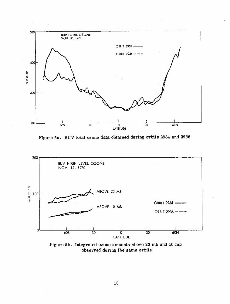
units above 20 mb, and becomes negligible above 10 mb. Again in Figure 5a a
similar marked increase in ozone may be noted at latitude 69S along the scan
path of orbit 2934, as compared with the observations during orbit 2936. The
corresponding changes at high level as seen in Figure 5b, are small above 20 mb
and really negligible above 10 mb. No doubt, it is better to study ozone maps
over extended areas whenever possible instead of individual orbits. Figures 6a
and 6b are the results of such a study. In the total ozone map of the Southern
14

60S 30S 0 30 60NLATITUDE
Figure 4c. BUV total ozone data obtained during orbits 2941 and 2939
60S 30 0
LATITUDE
30 60N
Figure 4d. Integrated ozone amounts above 20 mb and 10 mbcorresponding to the total ozone data in Figure 4c
15
500
400 -
E
EE
E
300 -
BUV TOTAL OZONENOV 13, 1970
ORBIT 2941
ORBIT 2939---
200
EU
EE
100 k
BUV HIGH LEVEL OZONENOV 13, 1970U
ORBIT 2941 -
ORBIT 2939
ABOVE 20 MB
. .. ABOVE 10 MB
ii .' I I- I- I
I I . I I' I
I
300
60S 30 0 30 60NLATITUDE
Figure 5a. BUV total ozone data obtained during orbits 2934 and 2936
100 -
60S 30 0LATITUDE
30 60N
Figure 5b. Integrated ozone amounts above 20 mb and 10 mbobserved during the same orbits
16
BUV TOTAL OZONENOV 12, 1970
ORBIT 2934
ORBIT 2936---
400
EEU
E
200
EU
E
BUV HIGH LEVEL OZONENOV. 12, 1970
ABOVE 20 MB
ORBIT 2934ABOVE 10 MB
ORBIT 2936 ---
_-0
---
I

4
j T O T A L OZONE S HEMISPHERE
MAY 10-11 ORBITS 427-452
Figure 6a. Total ozone chart for the Southern Hemisphere May 10-11
OZONE ABOVE 10 mt S HEMISPHERE
MAY 10-11 ORBITS 427-452
Figure 6b. Chart of ozone above 10 mb for the Southern Hemisphere May 10-11

Hemisphere for May 10-11 (Figure 6a) a high concentration appears at about
47S 100E corresponding to a vortex observable at this location in IDCS and THIR
imagery; this high concentration is not traceable in the corresponding chart
(Figure 6b) of ozone above 10 mb.
It would thus appear that in these cases the changes in ozone occur in the
lower stratosphere and possibly also to a small extent in the upper part of the
troposphere which is relatively poor in ozone. Little change occurs in the upper
stratosphere and mesosphere.
3. LONGITUDINAL INHOMOGENEITY IN THE TROPICAL BELT
On looking carefully at the cloud and ozone distribution in the tropical belt,
an interesting feature may be perceived. The chart of satellite relative cloud
cover in mean octas, for April of the years 1967-70 (Figure 7a) shows a well-
marked band of cloudiness just north of the equator (ITCZ), all round the globe
except between longitudes 30E to 70E. A similar band with essentially clear
skies over the African and adjoining Indian Ocean regions is discernible in the
charts for May and June 1967-70. (The June chart is reproduced in Figure 7b.)
Ozone values in the tropics are everywhere low, generally 250 +25 Dobson units.
But within the equatorial belt there is consistently somewhat higher ozone (about
10%) in the Indo-African region than over the rest of the belt, as is evident from
mean monthly ozone maps for April, May, June and July 1969 drawn from Nim-
bus 3 data (Prabhakara, Conrath, Allison and Steranka 1971). Figures 8a and 8b
display the maps for April and May. Many individual-day and short-term average
18

Figure 7a. Satellite cloud cover (mean octas) April 1967-70
eo Reproduced from best available copy.
Figure 7b. Satellite cloud cover (mean octas) June 1967-70

Figure 8a. Monthly mean ozone map (IRIS data) for April 1969
20
Figure 8b. Monthly mean ozone map (IRIS data) for May 1969

ozone maps also exhibit the same feature. IRIS total ozone map for April 23
(Figure 9), that for April 24 (Figure lc) and the BUV total ozone map for June
21-28 (Figure 10), are instances in point.
140 120 100 s0 60 40
so
60
30
20
t0
20
30
40
50
60
20
:OI0-t- ,16
$-
3
:3 39
- jbOjtt > (2~3
F0ir 201 -T 8- I 60 -0140_ 1. 20T , I , , , , 4010 120 10 80 60 ' 40.
0 20 40 60 80 100 120 140 160 IAI I I _ I I I I I I I I I I I I I I Ii~~~~~~~~~~~(' J, wZO %o J
I, * . I"6
11.j ~~~~~~--/4--,- _ _..._ -
W 4 1 C
t 36 300
I~~~~T
f~~~~~~~~~~~~~-- ;--F"10
~0
rTfi 7r-~T- 'I V~I-~f O0
-- 300 P DATA DAY 340
r -, , , T1 IT' I - r - X- 1- -1 ---i- -----r g0
3
20 0 20 40 60 fi t100 120 140 160 IRO I£0 140
OZONR DATA DAY 113
Figure 9. IRIS total ozone map of April 23, 1970
Evidently, there is a longitudinal inhomogeneity in the equatorial belt in
cloud as well as in ozone distribution. One may consider what possible atmos-
pheric circulations are consistent with this zonal asymmetry. It is well-known
that during these months the extensive, and world's-highest plateau over Tibet
21
go Ic I % o
I_,, (,,O i 1:
F<,' (" ';i _ __:'.. L~.-:t'
10,
M5 10 -j
0
4
C
.1
-1- I
'� q. I
,[I
I
I

BUV TOTAL OZONE (MILLI ATM - CM)
45°-< 250
U,-4 375 300 - ---30 0 ._ _3Z7K 4
•~~~250--
° 6C 65 -_ ____________________ - - - -90W 0 90E 180
LONGITUDE
Figure 10. BUV total ozone map for June 21-28
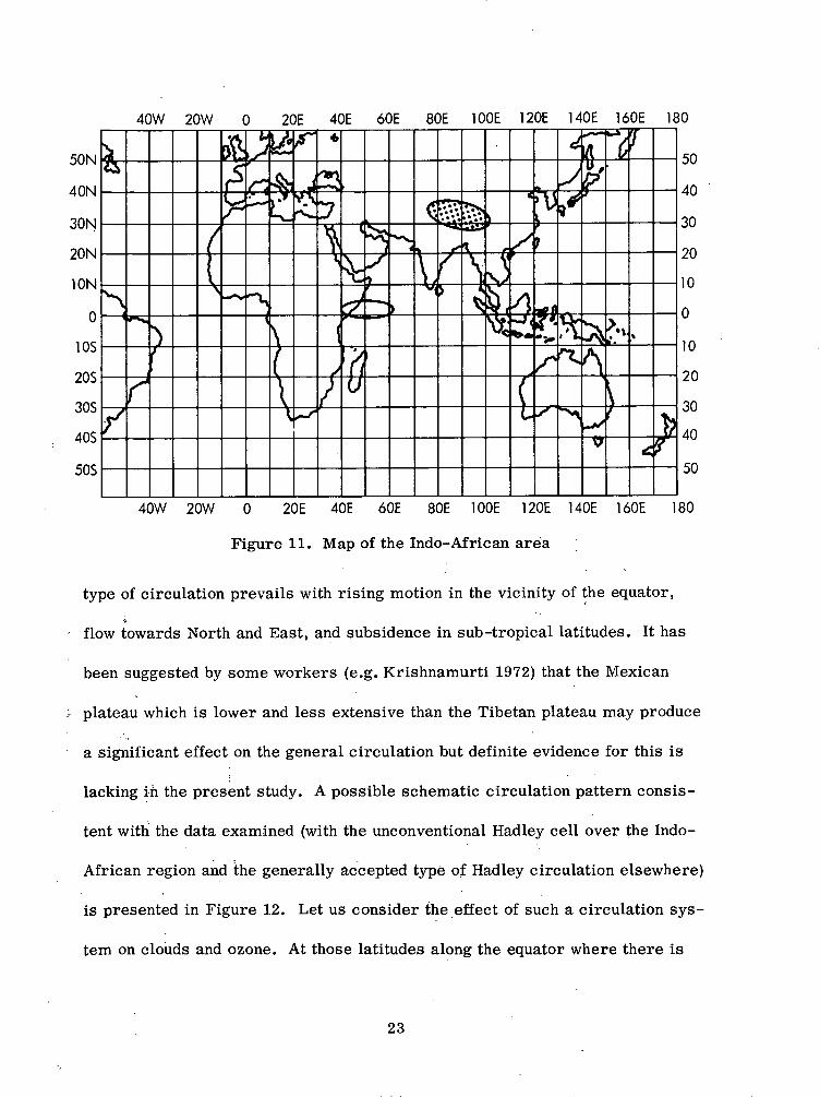
(see map in Figure 11) is heated by the sun to the point where it becomes a major
source of heat in the earth-atmospheric system. Koteswaram (unpublished) has
indicated that a meridional circulation prevails with air rising over Tibet at
about 30N and sinking close to the equator. This constitutes a reversed type of
Hadley cell locally in that particular part of the globe. While this cell is ther-
mally direct as in the usual Hadley circulation (the rising branch being at a
relatively higher temperature than the descending branch with consequent genera-
tion of kinetic energy), the sense of the circulation is opposed to that of the
normal Hadley cell in that the upper level flow here is southwards whereas it is
northwards in the regular Hadley circulation. Owing to coriolis force the plane
of the circulation has a NE-SW orientation, so that although air rises over Tibet
(80-100E) the downward motion takes place in the Indian Ocean close to the
African coast (40-60E). In other parts of the tropical belt, the traditional Hadley
22
DAY 172 -179 1970 78 ORBITS 21- 28 JUNE 1970
50N
40N
30N
20N
ION
0
o10S
20S
30S
40S
50S
40W 20W 0 20E 40E 60E 80E l OOE 120E 140E 160E 180
50... . .. , I _ __ _ _ _ 40
0 20E 40E 60E 80E 100 E 120E 140E
Figure 11. Map of the Indo-African area
type of circulation prevails with rising motion in the vicinity of the equator,
flow towards North and East, and subsidence in sub-tropical latitudes. It has
been suggested by some workers (e.g. Krishnamurti 1972) that the Mexican
plateau which is lower and less extensive than the Tibetan plateau may produce
a significant effect on the general circulation but definite evidence for this is
lacking in the present study. A possible schematic circulation pattern consis-
tent with the data examined (with the unconventional Hadley cell over the Indo-
African region and the generally accepted type of Hadley circulation elsewhere)
is presented in Figure 12. Let us consider the effect of such a circulation sys-
tem on clouds and ozone. At those latitudes along the equator where there is
23

\J
To N
.
cd
,ll4 ,'~
l
I r
I C
0l
I U
U
'
I YC
D
C.
I r
24
i 4,1!I :it4IIIII

downward motion, as may be expected, the skies are relatively cloud-free. As
for ozone, it is well established that there is no source of ozone of importance
below the tropopause. The tropopause derives its main supply of ozone from the
lower stratosphere of high latitudes (where ozone accumulates in winter) by the
process of mixing, mostly in spring, along isentropic surfaces, through the tro-
popause br.eak. The region round about 30N between 100 to 200 mb may thus be
regarded as an ozone source region, so far as the lower atmosphere is concerned.
Although ozone gets mixed in the troposphere by turbulence, the effect of a local
reversed Hadley cell would be a preferential transfer of ozone from the source
region at high levels around 30N to the zone where there is sinking air motion,
i.e., 40-60E. It is possible that the observed consistently higher ozone in the
Indo-African latitudes may be accounted for by this mechanism.
A comparison of the vertical distribution of ozone observed at Canal Zone
and Leopoldville (extracted from Hesstvedt 1965 and presented in Figure 13)
leads to the conclusion that the excess of ozone over Leopoldville is to be found
in the troposphere (while between 23 and 28 km there appears to be a relative
deficit). Furthermore, Griggs (1963) has reported on bubbler ozonesonde meas-
urements over Nairobi, which reveal rather low ozone concentrations over the
tropopause. These results do not favor an alternative mechanism (which one
may be tempted to consider) invoking transfer of ozone into the lower strato-
sphere over the African continent.
25

t25
II -
0I _ /UJ
20 _
//
1 2 3 4 5 6 7x1 012 cm-3
OZONE CONCENTRATION -
Figure 13. Vertical distributions of ozone observed over Canal Zoneand Leopoldville (after Hesstvedt)
Sea-surface temperatures during May 4 - June 2, 1970, deduced from
Nimbus 4 THIR data by Salomonson (unpublished) are presented in Figure 14.
One may see a minimum temperature of 24°C close to the equator between 40E
and 55E. The cause of this minimum is upwelling due to southwesterly surface
winds along the Somali coast. The SWwinds which occur over the area are con-
sistent with a reversed Hadley cell. In the light of the correlation between warm
26

seas and upward air-motion, the low temperature sea-area is compatible with
the atmospheric sink above.
+600.
*500
0400
+300
+100
00.0
-3 .0.0 .. .
-3 0 _
-40.0
00 ,10 20° 30o 400 500 60 700 800 90 100° 0 1 o00 o1200130o140o150o160o170,180o170o160o1501,40o130o120o110100 90o 800 700 600 50° 400 300 200 100 00
LONGITUDE IOEAST) LONGITUDE (°WEST)
Figure 14. Sea-surface temperatures during May 4-June 2, 1970deduced from Nimbus 4 THIR data
The transport of momentum by the reversed Hadley cell would be in the
sense opposite to that by the conventional Hadley circulation. The axis of the
sub-tropical westerly jet-stream is normally close to where the northward flow
at upper levels in the general Hadley cell ends, yielding to downward motion.
It is perhaps more than a coincidence that the axis of the, easterly jet stream
which is observed only in the Indo-African part of the tropics, is located nearly
where the southward flow at high levels in the reversed Hadley cell inferred
above, terminates (Figure 12).
The scheme put forward here is supported by some of the findings of Saha
(1971) who from a number of considerations deduces a zonal type of circulation
in the tropics with its descending limb at 45-55E. Saha's suggestion that the
27

ascent occurs over the eastern Indian Ocean does not, however, fit in with the
cloud, ozone and ocean surface temperature data examined in this study. Also,
Krishnamurti (1972), from a survey of global commercial aircraft reports, has
arrived at a distribution of velocity potential at 200 mb, with a peak value in the
tropics of 7 x 10⁶ meter2 sec 1 in the neighborhood of 20N 100E, the direction
of the steepest gradient from this potential hill, along which the airstream runs,
being southeastwards. There is thus broad agreement between this and the
present results, although the location of the potential peak is slightly to the
southeast of the Tibetan plateau at a place where it is difficult to think of an
immediate physical reason for high-level divergence.
4. WINDS AND OZONE GRADIENTS
Prabhakara, Rodgers and Salomonson (1973) have demonstrated a high cor-
relation between ozone amount and geopotential height, and deduced the geo-
strophic winds at 200 mb using total ozone as a quasi-stream function. Under-
standably, therefore, jet streams are associated with ozone gradients. During
the course of the present investigation, this association was observed to be
generally valid. Figure 15a presents the total ozone map of June 9, 1970, while
Figure 15b reproduces the 200 mb (1200z) chart of the same day. Between 42N
and 46N, 120E to 130E on that day the jet speed attains a maximum of 80-100 kt;
in the same area the ozone gradient is strong reaching a maximum value of 16
Dobson units per degree latitude. Similarly between 36 and 45N, 180 to 130W,
the jet again picks up speed to more than 80 kt and correspondingly the ozone
28

Figure 15a. Total ozone map for June 9, 1970
gradient in the region s t rengthens. Fur the rmore , the axis of the jet appears to
be covered at intervals (as in ea r l i e r instances) with little cells of ozone maxima.
These cells may be the resul t of clouds, or of eddies associated with the jet, or
of a wave pattern along the jet axis . In any event, the ozone gradient as well as
the cel ls of ozone maxima in the vicinity of the jet bear out ea r l i e r r e su l t s .
5. CONCLUDING REMARKS
In this investigation, resu l t s from a number of satell i te experiments en
abled a composite study being made of severa l types of data such as cloud, ozone
29

Figure 15b. 200 mb (1200z) chart of the same day
and sea-surface temperature. The main conclusions that may be drawn are:
1. (a) There is a close relationship between vortices in the troposphere
and maxima in total ozone.
(b) The enhancement in ozone associated with these vortices occurs
predominantly in the lower stratosphere.
2. (a) The equatorial belt exhibits longitudinal inhomogeneity in respect
of several meteorological parameters; it is marked by an area of
30

minimum cloudiness, comparatively high ozone and low sea-surface
temperature in the Indo-African region.
(b) A possible meridional circulation consistent with this inhomogeneity
is a reversed Hadley cell in summer locally over the Indo-African
area.
3. The association of high level winds with ozone gradients and of jet
streams with tiny cells of ozone maxima, is further substantiated.
It would be desirable to introduce a scanning device for ozone measuring
equipment on spacecraft; from the resulting improved data coverage more exact
conclusions could be drawn.
It is further suggested that a program may be undertaken (perhaps as a
part of GARP) to determine the vertical velocity (w) in the African and Indian
Ocean regions for verifying the reality of the reverse Hadley circulation. Prob-
ably the best procedure would be evaluation of w from the continuity equation,
horizontal divergence from the earth's surface upwards being derived from
winds measured by a close network of radar wind observing posts. Such data
would be invaluable in understanding the general circulation.
ACKNOWLEDGEMENTS
Thanks are due to V. V. Salomonson for permitting the use of sea-surface
temperature chart reproduced in Figure 14 and to L. J. Allison for supplying
Figure 15.
During the period of this investigation, M. S. V. Rao was the recipient of a
NRC-NASA Research Associateship.
31

REFERENCES
1. Hanel, R., Conrath, B., and Schlachman, B. "The Infrared Interferometer
Spectrometer Experiment." Nimbus 4 User's Guide, Goddard Space Flight
Center, Greenbelt, Md. (1970), 65-100
2. Heath, D., Krueger, A. J., and Mateer, C. "The Backscatter Ultraviolet
Spectrometer Experiment." Nimbus 4 User's Guide, Goddard Space Flight
Center, Greenbelt, Md. (1970) 149-169
3. Hesstvedt, E. "Ozone Distribution Over the EquSr and its Dependence
on Vertical Motions." Tellus, Vol. 17, No. 2 (1965) 177-178
4. Griggs, M. "Measurements of the Vertical Distribution of Atmospheric
Ozone at Nairobi." Quarterly Journal of the Royal Meteorological Society,
Vol. 89 (1963) 284-286
5. Koteswaram, P. (Unpublished) Indian Meteorological Service, New Delhi
6. Krishnamurti, T. N. "Observational Studies on Tropical General Circula-
tion." Final Report to NSF Grant No. GA 17822, Department of Meteorology,
Florida State University (1972)
7. McCulloch, A. W. "The Temperature-Humidity Infrared Radiometer Ex-
periment." Nimbus 4 User's Guide, Goddard Space Flight Center, Green-
belt, Md. (1970), 25-64
8. Prabhakara, C., Conrath, B. J., Allison, L. J. and Steranka, J. "Seasonal
and Geographical Variation of Atmospheric Ozone Derived from Nimbus 3."
NASA Technical Note D 6443 (1971)
32

9. Prabhakara, C., Rodgers, E. B., and Salomonson, V. V. "Remote Sensing
of Global Distribution of Total Ozone and the Inferred Upper Tropospheric
Circulation from Nimbus IRIS Experiments." Pure and Applied Geophysics
(1973)
10. Saha, K. R. "Cloud Distributions Over Equatorial Indian Ocean as Revealed
by Satellites." Indian Journal of Meteorology and Geophysics, Vol. 22 (1971)
389-396
11. Salomonson, V. V. (Unpublished). Goddard Space Flight Center, Greenbelt,
Md.
12. Werner, E. and Branchflower, G. A. "The Image Dissector Camera System."
Nimbus 4 User's Guide, Goddard Space Flight Center, Greenbelt, Md. (1970)
11-24
33
U.S. GOVERNMENT PRINTING OFFICE: 1972-735.966/540