to accompany principles of highway engineering...

Solutions Manual to accompany

Principles of Highway Engineering and Traffic Analysis, 4e

By Fred L. Mannering, Scott S. Washburn, and Walter P. Kilareski

Chapter 2 Road Vehicle Performance

U.S. Customary Units

Copyright © 2008, by John Wiley & Sons, Inc. All rights reserved.

Solutions Manual to accompany Principles of Highway Engineering and Traffic Analysis, 4e, by Fred L. Mannering, Scott S. Washburn, and Walter P. Kilareski. Copyright © 2008, by John Wiley & Sons, Inc. All rights reserved.

Preface The solutions to the fourth edition of Principles of Highway Engineering and Traffic Analysis were prepared with the Mathcad1 software program. You will notice several notation conventions that you may not be familiar with if you are not a Mathcad user. Most of these notation conventions are self-explanatory or easily understood. The most common Mathcad specific notations in these solutions relate to the equals sign. You will notice the equals sign being used in three different contexts, and Mathcad uses three different notations to distinguish between each of these contexts. The differences between these equals sign notations are explained as follows.

• The ‘:=’ (colon-equals) is an assignment operator, that is, the value of the variable or expression on the left side of ‘:=’is set equal to the value of the expression on the right side. For example, in the statement, L := 1234, the variable ‘L’ is assigned (i.e., set equal to) the value of 1234. Another example is x := y + z. In this case, x is assigned the value of y + z.

• The ‘==’ (bold equals) is used when the Mathcad function solver was used to find the value of a variable in the equation. For example, in the equation

, the == is used to tell Mathcad that the value of the expression on the left side needs to equal the value of the expression on the right side. Thus, the Mathcad solver can be employed to find a value for the variable ‘t’ that satisfies this relationship. This particular example is from a problem where the function for arrivals at some time ‘t’ is set equal to the function for departures at some time ‘t’ to find the time to queue clearance.

• The ‘=’ (standard equals) is used for a simple numeric evaluation. For example, referring to the x := y + z assignment used previously, if the value of y was 10 [either by assignment (with :=), or the result of an equation solution (through the use of ==) and the value of z was 15, then the expression ‘x =’ would yield 25. Another example would be as follows: s := 1800/3600, with s = 0.5. That is, ‘s’ was assigned the value of 1800 divided by 3600 (using :=), which equals 0.5 (as given by using =).

Another symbol you will see frequently is ‘→’. In these solutions, it is used to perform an evaluation of an assignment expression in a single statement. For example, in the following

statement, , Q(t) is assigned the value of Arrivals(t) – Departures(t), and this evaluates to 2.2t – 0.10t2. Finally, to assist in quickly identifying the final answer, or answers, for what is being asked in the problem statement, yellow highlighting has been used (which will print as light gray). 1 www.mathcad.com


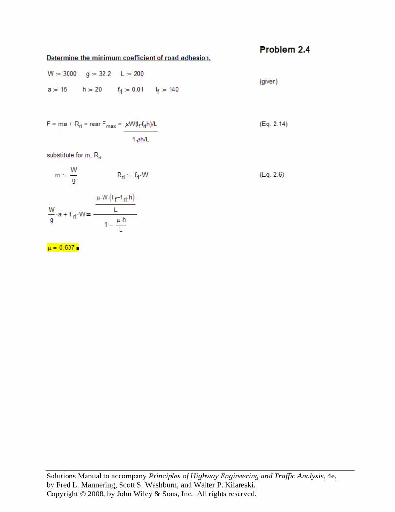
Determine the maximum grade. Problem 2.11

i 0.035:= ne350060

:= εo 3.2:= r1412

:= W 2500:= lb (given)

assume F=Fe

calculate velocity

(Eq. 2.18) V

2 π⋅ r⋅ ne⋅ 1 i−( )⋅

εo:= V 128.9= ft/s

calculate aerodynamic resistance

ρ 0.002378:= CD 0.35:= Af 25:=

(Eq. 2.3)Ra

ρ

2CD⋅ Af⋅ V 2

⋅:= Ra 172.99= lb

calculate rolling resistance

frl 0.01 1V

147+

⎛⎜⎝

⎞⎟⎠

:= (Eq. 2.5)

Rrl frl W⋅:= Rrl 46.93= lb

calculate engine-generated tractive effort

Me 200:= nd 0.90:=

(Eq. 2.17)Fe

Me εo⋅ nd⋅

r:= Fe 493.71= lb

calculate grade resistance

Rg Fe Ra− Rrl−:= (Eq. 2.2)

Rg 273.79=

solve for G

GRgW

:= (Eq. 2.9)

G 0.1095= therefore G = 11.0%


Alternative calculation for grade, using trig relationships

θg asinRgW

⎛⎜⎝

⎞⎟⎠

:=

θg 0.1097= radians

degθg θg180π

⋅:= convert from radians to degrees

degθg 6.287=

tan deg = opposite side/adjacent side

G tan θg( ) 100⋅:= G 11.02= %

Thus, error is minimal when assuming G = sin θg for small to medium grades


Problem 2.12 Determine the torque the engine is producing and the engine speed.

Fe ΣR− γm m⋅ a⋅

at top speed, acceleration = 0; thus, Fe ΣR− 0

V 12452803600⋅:= V 181.867= ft/s (given)

calculate aerodynamic resistance

ρ 0.00206:= CD 0.28:= Af 19.4:=

Raρ

2CD⋅ Af⋅ V 2⋅:= Ra 185.056= (Eq. 2.3)

calculate rolling resistance

frl 0.01 1V

147+

⎛⎜⎝

⎞⎟⎠

⋅:= frl 0.022= (Eq. 2.5)

W 2700:= (given)

(Eq. 2.6)Rrl frl W⋅:= Rrl 60.404=

Rg 0:=

sum of resistances is equal to engine-generated tractive effort, solve for Me

(Eq. 2.2)Fe Ra Rrl+ Rg+:= Fe 245.46=

i 0.03:= ηd 0.90:= ε0 2.5:= r12.612

:=

(Eq. 2.17)Fe

Me ε0⋅ ηd⋅

rMe

Fe r⋅

ε0 ηd⋅:=

Me 114.548= ft-lb

Knowing velocity, solve for ne

(Eq. 2.18)V

2 π⋅ r⋅ ne⋅ 1 i−( )⋅

ε0ne

V ε0⋅

2 π⋅ r⋅ 1 i−( )⋅:=

ne 71.048=

revs

ne 60⋅ 4263=revmin


Rear - wheel drive

μ 0.2:= frl 0.011:= h 20:= L 120:= lf 60:=


Salγb V1

2 V22

−⎛⎝

⎞⎠⋅

2 g⋅ ηb μm⋅ frl 0.03−+( )⋅(Eq. 2.43)

V2 V12 2 Sal⋅ g⋅ ηb μm⋅ frl+ 0.03−( )⋅

γb−:=


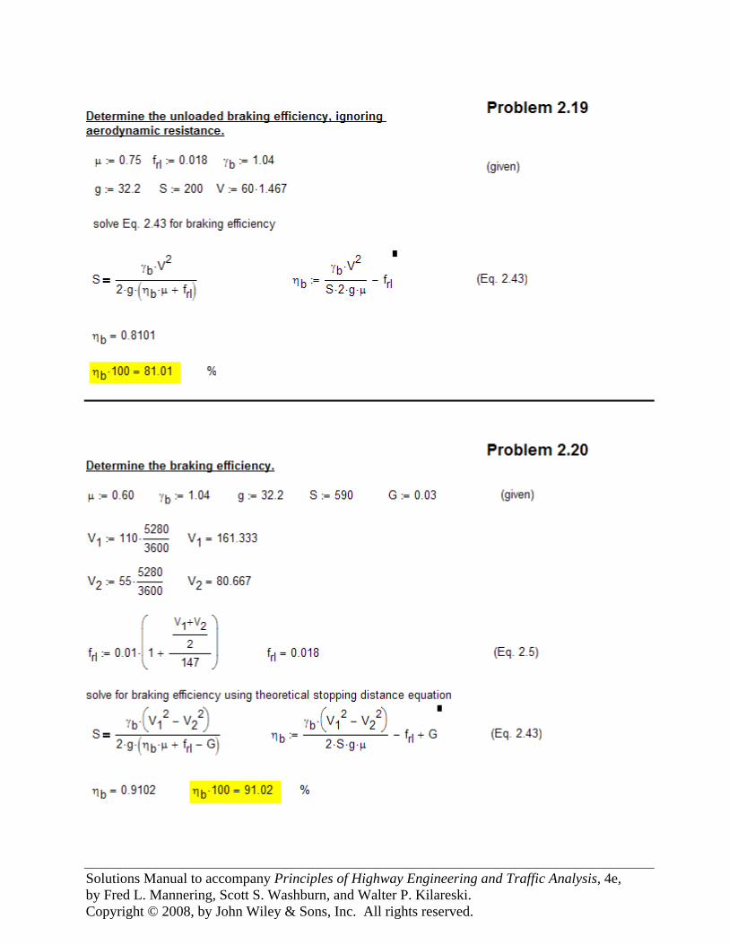
Problem 2.24 Determine if the driver should appeal the ticket.

μ 0.6:= (for good, wet pavement, and slide value because of skidding)

γ b 1.04:= g 32.2:=

V2 4052803600⋅:= V2 58.667= (given)

ηb 0.95:= S 200:= frl 0.015:=

Solve for the initial velocity of the car using theoretical stopping distance

Sγ b V1

2 V22

−⎛⎝

⎞⎠⋅

2 g⋅ ηb μ⋅ frl+ 0.04−( )⋅V1

2 S⋅ g⋅ ηb μ⋅ frl+ 0.04−( )⋅

γ bV2

2+:= (Eq. 2.43)

V1 100.952=

V136005280⋅ 68.83=

mih

No, the driver should not appeal the ticket as the initial velocity was higher than the speed limit,in addition to the road being wet.


G 0.059= G 100⋅ 5.93= %


Multiple Choice Problems Determine the minimum tractive effort. Problem 2.31

CD 0.35:= Af 20:= ft2 ρ 0.002045:=slugs

ft3 (given)

V 7052803600

⎛⎜⎝

⎞⎟⎠

⋅:=fts

W 2000:= lb

G 0.05:=

grade resistance

Rg 2000 G⋅:= Rg 100= lb (Eq. 2.9)

aerodynamic resistance

Raρ

2CD⋅ Af⋅ V2

⋅:= Ra 75.44= lb (Eq. 2.3)

rolling resistance

frl 0.01 1V

147+⎛⎜

⎝⎞⎟⎠

⋅:= frl 0.02= (Eq. 2.5)

Rrl frl W⋅:= Rrl 33.97= lb (Eq. 2.6)

summation of resistances

(Eq. 2.2)F Ra Rrl+ Rg+:= F 209.41= lb


−−−−−−−−−−−−−−−−−−−−−−−−−−−−−−−−−−−−−−−−−−−−−−−−−−−−−−−−−−−Alternative Answers:

1) Using mi/h instead of ft/s for velocity

V 70:=mih

frl 0.01 1V

147+⎛⎜

⎝⎞⎟⎠

⋅:= frl 0.01=

Rrl frl W⋅:= Rrl 29.52= lb

Raρ

2CD⋅ Af⋅ V2

⋅:= Ra 35.07= lb

F Ra Rrl+ Rg+:= F 164.6= lb

2) not including aerodynamic resistance

V 7052803600⋅:=

F Rrl Rg+:= F 129.52= lb

3) not including rolling resistance

F Ra Rg+:= F 135.07= lb


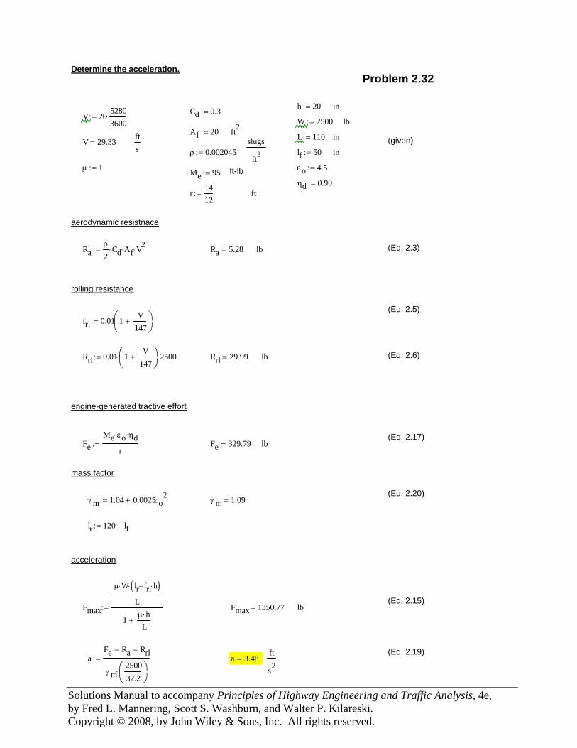
Determine the acceleration.Problem 2.32

h 20:= inCd 0.3:=V 2052803600⋅:= W 2500:= lb

Af 20:= ft2 L 110:= inV 29.33=fts

(given)slugs

ft3ρ 0.002045:= lf 50:= in

μ 1:= εo 4.5:=Me 95:= ft-lbηd 0.90:=

r1412

:= ft

aerodynamic resistnace

Raρ

2Cd⋅ Af⋅ V2

⋅:= Ra 5.28= lb (Eq. 2.3)

rolling resistance

(Eq. 2.5)frl 0.01 1

V147

+⎛⎜⎝

⎞⎟⎠

:=

Rrl 0.01 1V

147+⎛⎜

⎝⎞⎟⎠

⋅ 2500⋅:= Rrl 29.99= lb (Eq. 2.6)

engine-generated tractive effort

(Eq. 2.17)Fe

Me εo⋅ ηd⋅

r:= Fe 329.79= lb

mass factor

(Eq. 2.20)γ m 1.04 0.0025εo

2+:= γ m 1.09=

lr 120 lf−:=

acceleration

(Eq. 2.15)Fmax

μ W⋅ lr frl h⋅+( )⋅

L

1μ h⋅L

+

:= Fmax 1350.77= lb

(Eq. 2.19)a

Fe Ra− Rrl−

γ m250032.2

⎛⎜⎝

⎞⎟⎠

⋅

:= a 3.48=ft

s2



ft

s21) Use a mass factor of 1.04 γ m 1.04:= aFe Ra− Rrl−

γ m250032.2

⎛⎜⎝

⎞⎟⎠

⋅

:= a 3.65=

2) Use Fmax instead of Feft

s2γ m 1.091:= aFmax Ra− Rrl−

γ m250032.2

⎛⎜⎝

⎞⎟⎠

⋅

:= a 15.53=

3) Rear wheel instead of front wheel drive

Fmax

μ W⋅ lf frl h⋅−( )⋅

L

1μ h⋅L

−

:= Fmax 1382.22= aFmax Ra− Rrl−

γ m250032.2

⎛⎜⎝

⎞⎟⎠

⋅

:= a 15.9=ft

s2


Determine the percentage of braking force. Problem 2.33

V 6552803600⋅:=

fts

μ 0.90:=

L 120:= in lf 50:= in (given)

h 20:= in lr L lf−:= in

determine the coefficient of rolling resistance

(Eq. 2.5)frl 0.01 1

V147

+⎛⎜⎝

⎞⎟⎠

⋅:= frl 0.02=

determine the brake force ratio

BFRfrmaxlr h μ frl+( )⋅+

lf h μ frl+( )⋅−:= BFRfrmax 2.79= (Eq. 2.30)

calculate percentage of braking force allocated to rear axle

PBFr100

1 BFRfrmax+:= PBFr 26.39= % (Eq. 2.32)


1) Use front axle equation

PBFf 100100

1 BFRfrmax+−:= PBFf 73.61= % (Eq 2.31)

2) Use incorrect brake force ratio equation

BFRfrmaxlr h μ frl+( )⋅−

lf h μ frl+( )⋅+:= BFRfrmax 0.76=

PBFr100

1 BFRfrmax+:= PBFr 56.94= %

3) Switch l f and lr in brake force ratio equation

BFRfrmaxlf h μ frl+( )⋅+

lr h μ frl+( )⋅−:= BFRfrmax 1.32=

PBFr100

1 BFRfrmax+:= PBFr 43.06= %


Determine the theoretical stopping distance on level grade. Problem 2.34

CD 0.59:= V 8052803600⋅:=

fts (given)

Af 26:= ft2 μ 0.7:=

γ b 1.04:= ηb 0.75:= (assumed values)

Coefficient of Rolling Resistance

(Eq. 2.5) frl 0.01 1

V

2

147+

⎛⎜⎜⎝

⎞⎟⎟⎠

⋅:= frl 0.014=

Theoretical Stopping Distance

(Eq. 2.43)S

γ b V12 V2

2−⎛

⎝⎞⎠⋅

2 g⋅ ηb μ⋅ frl+( )⋅:= S 412.8

s2

ft=

−−−−−−−−−−−−−−−−−−−−−−−−−−−−−−−−−−−−−−−−−−−−−−−−−−−−−−−−

Alternative Answers:

1) Not dividing the velocity by 2 for the coeffeicent of rolling resistance

frl 0.01 1V

147+⎛⎜

⎝⎞⎟⎠

⋅:=

Sγ b V1

2 V22

−⎛⎝

⎞⎠⋅

2 g⋅ ηb μ⋅ frl+( )⋅:= S 409.8

s2

ft=

2) Using mi/h instead of ft/s for the velocity

V1 80:= V2 0:= V 80:=

frl 0.01 1

V

2

147+

⎛⎜⎜⎝

⎞⎟⎟⎠

⋅:=

Sγ b V1

2 V22

−⎛⎝

⎞⎠⋅

2 g⋅ ηb μ⋅ frl+( )⋅:= S 192.4

s2

ft=


3) Using γ = 1.0 value

γ b 1.0:=

Sγ b V1

2 V22

−⎛⎝

⎞⎠⋅

2 g⋅ ηb μ⋅ frl+( )⋅:= S 397.9

s2

ft=

Determine the stopping sight distance. Problem 2.35

V 4552803600⋅:= ft/s (given)

a 11.2:=ft

s2tr 2.5:= s g 32.2:=

ft

s2assumed( )

Braking Distance

(Eq. 2.47)d

V2

2 g⋅ag

⎛⎜⎝

⎞⎟⎠

⋅

:= d 194.46= ft

Perception/Reaction Distance

(Eq. 2.49)dr V tr⋅:= dr 165.00= ft

Total Stopping Distance

(Eq. 2.50)ds d dr+:= ds 359.46= ft


1) just the braking distance value

d 194.46= ft

2) just the perception/reaction distance value

dr 165.00= ft


3) use the yellow signal interval deceleration rate

a 10.0:=

dV2

2 g⋅ag

⎛⎜⎝

⎞⎟⎠

⋅

:= d 217.80= ft

ds d dr+:= ds 382.80= ft

Determine the vehicle speed. Problem 2.36

CD 0.35:= G 0.04:= γ b 1.04:=

Af 16:= ft2 S 150:= ft ηb 1:= (given)

W 2500:= lbslugs

ft3ρ 0.002378:= μ 0.8:=

V1 8852803600⋅:=

fts frl 0.017:=g 32.2:=

ft

s2

Kaρ

2CD⋅ Af⋅:= Ka 0.007=

Given

V2 0:=

(Eq. 2.39)S

γ b W⋅

2 g⋅ Ka⋅ln

ηb μ⋅ W⋅ Ka V12

⋅+ frl W⋅+ W G⋅+

ηb μ⋅ W⋅ Ka V22⎛

⎝⎞⎠⋅+ frl W⋅+ W G⋅+

⎡⎢⎢⎣

⎤⎥⎥⎦

⋅

V2 Find V2( ):=

V2 91.6=V2

1.46762.43=

mih

−−−−−−−−−−−−−−−−−−−−−−−−−−−−−−−−−−−−−−−−−−−−−−−−−−−−−−−


−−−−−−−−−−−−−−−−−−−−−−−−−−−−−−−−−−−−−−−−−−−−−−−−−−−−−Alternative Answers:

1) Use 0% grade

G 0.0:=

Given

V2 0:=

Sγ b W⋅

2 g⋅ Ka⋅ln

ηb μ⋅ W⋅ Ka V12

⋅+ frl W⋅+ W G⋅+

ηb μ⋅ W⋅ Ka V22⎛

⎝⎞⎠⋅+ frl W⋅+ W G⋅+

⎡⎢⎢⎣

⎤⎥⎥⎦

⋅

V2 Find V2( ):=

V2 93.6=V2

1.46763.78=

mih

2) Ignoring aerodynamic resistance

G 0.04:=

(Eq 2.43) rearranged tosolve for V2

V2 V12 S 2⋅ g⋅ ηb μ⋅ frl+ G+( )⋅

γ b−:= V2 93.3=

V21.467

63.6=mih

3) Ignoring aerodynamic resistance and using G = 0

G 0:=

V2 V12 S 2⋅ g⋅ ηb μ⋅ frl+ G+( )⋅

γ b−:= V2 95.2=

V21.467

64.9=mih

to accompany principles of highway engineering...

Documents