to design and implement data mining application by … design and implement data mining application...

@IJMTER-2015, All rights Reserved 208

To Design and Implement Data Mining Application By using Top

Down Approach

Rakhi Satam

PG in Mtech Computers,Department of Computer,Science & Engineering,Veermata Jijabai

Technological Institute, Matunga, Mumbai

Abstract—This paper presents how clusters are made by using Partitional algorithms. In Partitional

algorithms k-means and k-medoid plays an important role. Firstly partition can be made by using k-

means or k-medoid. Secondly after forming partition which objects fall under which clusters can be

viewed by using searching.

Index Terms—Clustering, forensic computing, text mining

I. INTRODUCTION

High-dimensional data is a phenomenon in real-world data mining applications. Text data is a typical

example. In text mining, a text document is viewed as a set of pairs <ti, fi>, where ti is a term or word,

and fi is a term or word and fi is a measure of ti,for example, the frequency of ti in the document. The

total number of unique terms in a text data set represents the number of dimensions, which is usually

in the thousands. High- dimensional data occurs in business as well. In retail companies, for example,

for effectiveness supplier relationship management (SRM), suppliers are often categorized in groups

according to their business behaviors. The supplier's behavior data is high dimensional because

thousands of attributes are used to describe the supplier's behaviors, including product items, ordered

amounts,order frequencies, product quality and so on. Sparsity is an accompanying phenomenon of

high-dimensional data. In text data, documents related to a particular topic, for instance medicine are

categorized by one subset of terms. The terms describing medicine may not occur in the documents

describing music. This implies that fi is zero for the subset of terms in the documents describing

music and vice versa. Such situation also occurs in suppliers categorization. A group of suppliers are

categorized by the subset of product items supplied by the suppliers. Other suppliers who did not

supply these product items have zero order amount for them in the behavior data. Clearly, clustering

of high dimensional sparse data requires special treatment . This type of clustering methods is referred

to as subspace clustering, aiming at finding clusters from subspaces of data instead of the entire data

space. In a subspace clustering, each cluster is a set of objects identified by a subset of dimensions

and different clusters are represented in different subsets of dimensions. The major challenge of

subspace clustering which makes it distinctive from traditional clustering,is the simultaneous

determination of both cluster memberships of objects and the subspace of each cluster.

Cluster memberships are determined by the similarities of objects measured with respect to subspaces.

II. RELATED WORK

There are only a few studies reporting the use of clustering algorithms in the computer Forensics field.

Essentially, most of the studies describe the use of classic algorithms for clustering data example:-

Expectation–Maximization(EM) for unsupervised learning of Gaussian Mixture Models, K-

means,Fuzzy C-means (FCM) and self-organizing Maps(SOM). These algorithms have well-known

properties and are widely used in practice. For instance, k-means and FCM can be seen as particular

cases of EM. SOM–based algorithms were used for clustering files with the aim of making the

decision -making process performed by the examiners more efficient. One of these algorithms had

been used for query searching. Particular word falls under which cluster of documents can be found

International Journal of Modern Trends in Engineering and Research (IJMTER) Volume 02, Issue 06, [June– 2015] ISSN (Online):2349–9745 ; ISSN (Print):2393-8161


by using such algorithms. Fuzzy c-means algorithm can be used for association rules. This algorithm

is used for marketing based datasets. The most common approach to finding association rules is to

break up the problems into 2 parts:-

1. Find large item sets whose number of occurrences is above a threshold.

2. Generate rules from frequent item sets.

But most of the association rules deal with bottom up approaches. In bottom up approaches most of

algorithms deals with recursive method which in unnecessary takes memory space.

III. STEPS FOR DATA MINING OF RESULTS

A] Datasets:- we used five datasets obtained from real-world investigation cases conducted by the Brazilian Federal

police Department. Each dataset was obtained from a different hard drive,being selected all the non

duplicate documents with extensions “doc”, “docx” and “odt”. Subsequently, those documents were

converted into plain text format and then be preprocessed.

B] Pre - processing steps. Before running clustering algorithms on documents,we have to perform some preprocessing steps.

Stopwords like prepositions, pronouns, articles and irrelevant document metadata have been removed.

Also, the snowball stemming algorithm for portuguese words has been used. Then, we adopted a

traditional statistical approach for text mining, in which documents are represented in a vector space

model. In this model,each document is represented by a frequency occurences of words,which are

defined as delimited alphabetic strings,whose number of characters is between 4 and 25.

C] Clustering algorithms:- After doing all preprocessing steps now data is clean. It's time to do data partitions.

Data partition can be done by using two algorithms.

K-means

K-medoid

Object belonging k-means is one of the simplest unsupervised learning algorithms that solve the well

known clustering problem. The procedure follows a simple and easy way to classify a given data set

through a certain number of clusters (assume k clusters) fixed a priori. The main idea is to define k

centroids, one for each cluster. These centroids should be placed in a proper way because of different

location causes different result. So, the better choice is to place them as much as possible for away

from eachother. The next step is to take each point belonging to a given dataset and associate it to the

nearest centroid. When no point is pending, the first step is completed and an early groupage is done.

At this point, we need to re-calculate k new centroids as centers of the clusters resulting from the

previous step. After we have these k new centroids a new binding has to be done between the same

data set points and the nearest new centroid. A loop has been generated. As a result of this loop we

may notice that the k centroids change their location step by step until no more changes are done. In

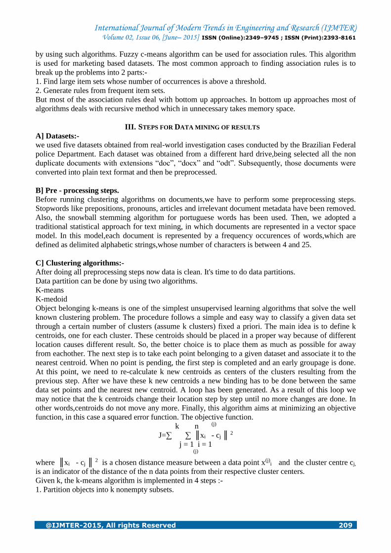
other words,centroids do not move any more. Finally, this algorithm aims at minimizing an objective

function, in this case a squared error function. The objective function.

k n (j)

J=∑ ∑ ║xi - cj ║ 2

j = 1 i = 1 (j)

where ║xi - cj ║ 2 is a chosen distance measure between a data point x(j)i and the cluster centre cj,

is an indicator of the distance of the n data points from their respective cluster centers.

Given k, the k-means algorithm is implemented in 4 steps :-

1. Partition objects into k nonempty subsets.



2. Compute seed points as the centroids of the clusters of the current partition. The centroid is the

center (mean point) of the cluster.

3.Assign each object to the cluster with the nearest seed point.

4. Go back to step 2, stop when no more new assignment.

K - medoids or PAM(partition around medoids) :- Each cluster is represented by one of the objects in

the cluster. Instead of taking the mean value of the object in a cluster as a reference point, medoids

can be used, which is the most centrally located object in a cluster.

(I) Also called as partitioning Around Medoids (PAM).

(II)Handles outliers well.

(III)Ordering of input does not impact results.

(IV)Does not scale well.

(V)Each cluster represented by one item,called the medoid.

(VI)Initial set of k medoids randomly chosen.

Therefore k-medoid can be used for applications

1) Centroids cannot be computed.

2)Distances between pairs of objects are available, as for computing dissimilarities between names of

documents with the Levenshtein distance. Unlike the partitional algorithms such as k-means/medoids,

hierarchical algorithms such as single/complete/average link provide a hierarchical set of nested

partitions usually represented in the form of a dendrogram.

D] Estimating the Number of clusters From Data In order to estimate the number of clusters, a widely used approach consists of getting a set of data

partitions, with different numbers of clusters and then selecting that particular partition that provides

the best result according to a specific quality criterion (eg. A relative validity index). Such a set of

partitions may result directly from a hierarchical clustering dendrogram or alternatively from multiple

runs of a partitional algorithm (eg. K- means) starting from different numbers and enitial positions of

the cluster prototypes.

A set of data partitions with different numbers of clusters is available, from which we want to choose

the best one-according to some relative validity criterion. By choosing such a data partition, we are

performing model selection and as an intrinsic part of this process, we are also estimating the number

of clusters.

A widely used relative validity index is the so-called silhouette which has also been adopted as a

component of the algorithms.

Eg:- Let us consider an object I belonging to cluster A. The average dissimilarity of I to all other

objects of A is denoted by a(i). Let us take into account cluster B. The average dissimilarity of I to all

objects of B will be called d(i,B). After computing d(i,B) for all clusters B ≠ A. This value represents

the dissimilarity of i to its neighbor cluster, and the silhouette for given object, S(i) is given by

S(i) = b(i)- a(i) …....................................(1)

max{a(i),b(i)}

It can be verified that -1≤ S(i) ≤ 1. Thus, the higher s(i) the better the assignment of object I to a given

cluster.

If s(i) = 0 , then it is not clear whether the object should have been assigned to its current cluster or to

a neighboring one.

Finally, if cluster A is a singleton, then s(i) is not defined and most neutral choice is to set s(i) = 0.

Once we have computed s(i) over i=1,2,....N where N is the number of objects in the dataset, we take

the average over these values, and the resulting value is then a quantitative measure of the data

partition in hand. Thus, the best clustering corresponds to the data partition that has the maximum

average silhouette.



There are two types of silhouette

Average Silhouette

Simplified Silhouette.

The average silhouette depends on the computation of all distances among all objects. To come up

with a more computationally efficient criterion, called simplified silhouette, one can compute only the

distances among the objects and the centroids of the clusters. The term a(i) of (1) now corresponds to

the dissimilarity of object I to its corresponding cluster (A) centroid.

E] Dealing with similarity and dissimilarity For checking similarity between documents we use cosine similarity measure.

It is from -1 < 0 < 1. while checking between similarity between documents we use vector model as it

deals with frequencies of words. After dealing with particular words and letters that particular words

are checked with next document and so on. At last similarity can be measured Minimum similarity

more will be dissimilarity and it can be shown by cosine waveform .

Figure 1: Cosine Waveform

for similarity matrix we have implemented incremented mining algorithm. This deal with similarity

vector.

δ(σn , cn)

σ – document

c – Cluster

n - Number

As we have seen while deciding which cluster is best in section III – D silhouette there we have used

δ(i,β) we are dealing with objects but here we are dealing with documents under cluster.

IV. COMPARING FOR PURITY BETWEEN CLUSTERING ALGORITHMS

While dealing with cluster we used two ways by using partitional algorithm and other by using

hierarchical algorithms. But as we had discuss silhouette is more used for similarity purpose. So, we

had going to show purity and check which way is better.

Thus it can be shown by the graph that as compared to k-means incremental mining algorithm which

has silhouette equation in built gives more pure results.

A. Correlation "Distances" and Hierarchical Clustering

There are many ways to perform hierarchical clustering in R, but a "controlled" experiment

may be useful in understanding which methods may be more useful when analyzing experimental

data.

This Technote explains an R experiment where data with "known" correlations are analyzed to

create a hierarchical clustering.

Some of the results presented here should be useful in analyzing experimental data when the

"answer" is not known.

Creating random values in R is easy with its various random number generators. We could

create completely random data to analyze, but the approach here is to create pairs of data variables



with known correlations ranging from 0.0 (completely uncorrelated) to 1.0 (complete correlated).

Actually, the correlation range from -1.0 to +1.0 will be spanned by picking pairs of values with these

correlations: 0.0, -0.20, +0.40, -0.60, +0.80, -1.00. How can random values with known correlations

be computed?

V. HIERARCHICAL CLUSTERING METHODS

A basic algorithm for finding the hierarchical clustering will be described. The nature of the algorithm

is agglomerative: First there are as many clusters as there are subjects, then the two clusters which are

closest are joined, repeatedly, and eventually all subjects have been joined in a single cluster.

In more detail the algorithm consists of the following steps

1. Define each subject as a group with dissimilarity $ D_{ij}$ between subjects $ i$ and $ j$ .

2. Find smallest element in $ D$ , $ D_{km}$ ($ k \ne m$ ) say. Join the groups $ k$ and $ m$

into the group $ \{k,m\}$ (the two closest groups are united).

3. Calculate the dissimilarity between the new group consisting of $ \{k, m\}$ and the

remaining groups. Form a new dissimilarity matrix.

4. Go through steps 2 and 3 until all subjects have been joined.

There are many rules for deciding how the combined units should be treated. The rules are all based

on the notion linkage, the features of the two groups joined carried over to the union of the groups

(how are the groups linked together?).

We will consider three methods for calculating the dissimilarity of a union of groups.

single linkage

complete linkage

average linkage

The single-linkage method, also called nearest-neighbour method, calculates the dissimilarity between

the new group $ \{k, m\}$ and any other group $ l$ as the minimum of the two dissimilarities $

D_{kl}$ and $ D_{ml}$ . This form of linkage means that a single link is enough to join to groups,

and this feature will allow clusters to be elongated and not necessarily spherical.

The complete-linkage method or furthest-neighbour method takes the maximum of the two

dissimilarities $ D_{kl}$ and $ D_{ml}$ as the new dissimilarity. Complete-linkage implies that

clusters are formed on the basis of the maximum dissimilarities between the clusters, and this tend to

produce spherical clusters.

In the average linkage method, also called unweighted pair-group method using arithmetic averages

(UPGMA), the dissimilarity between groups $ k/m$ and $ l$ is defined as the average of the two

dissimilarities $ D_{kl}$ and $ D_{ml}$ . The average linkage method also leads to spherically-

shaped clusters.



A. Dendrograms

The cluster solution from a hierarchical clustering method can be displayed in a two-dimensional plot,

in a dendrogram or tree diagram. A tree is a collection of clusters such that any two clusters either are

disjoint or one contains the other. The largest cluster, which is the set of all $ n$ units, contains all

other clusters, and the smallest clusters are the individual units.

The dendrogram is the two-dimensional representation of the tree. Usually it is displayed with the

largest cluster (containing all units) at the top and the smallest clusters (the units) at the bottom, being

a tree up-side-down; see Figure 2.2. The dendrogram provides an overview on the cluster solution,

and any horizontal cut of the dendrogram will yield a number of clusters. For instance, a cut a 7.5 on

the y axis in Figure 2.2 will divide the four units into two clusters (one cluster with one unit and one

cluster with three units), whereas a cut at 3.5 will result in three clusters (two clusters with one unit

each and one cluster with two units). The dissimilarities used in the clustering method correspond to

the lengths of the edges. Therefore the dendrogram provides a way to determine the number of

clusters by looking at the heights. A particular clustering is obtained by cutting the tree at some

specific height. Large heights may suggest reasonably well-separated clusters, but deciding where to

cut the tree still contains an element of subjective judgment.

a) Determining the number of clusters: As already mentioned a hierarchical clustering method

yields a cluster solution which contains clustering with any number of clusters between 1 and $ n$ .

In addition to the visual assessment using the dendrogram some statistics are available for

determining the number of clusters. We consider two statistics: The root-mean-square standard

deviation (RMSSTD) and R-square (RS). RMSSTD is a measure of homogeneity within clusters,

and RS indicates the extent to which clusters are different from each other.

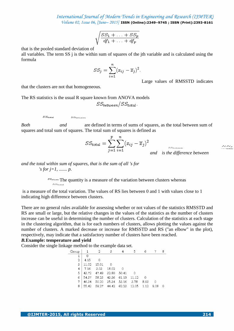
The RMSSTD statistic is the value of



that is the pooled standard deviation of

all variables. The term SS j is the within sum of squares of the jth variable and is calculated using the

formula

Large values of RMSSTD indicates

that the clusters are not that homogeneous.

The RS statistics is the usual R square known from ANOVA models

Both and are defined in terms of sums of squares, as the total between sum of

squares and total sum of squares. The total sum of squares is defined as

and is the difference between

and the total within sum of squares, that is the sum of all 's for

's for j=1, ....... p.

The quantity is a measure of the variation between clusters whereas

is a measure of the total variation. The values of RS lies between 0 and 1 with values close to 1

indicating high difference between clusters.

There are no general rules available for assessing whether or not values of the statistics RMSSTD and

RS are small or large, but the relative changes in the values of the statistics as the number of clusters

increase can be useful in determining the number of clusters. Calculation of the statistics at each stage

in the clustering algorithm, that is for each numbers of clusters, allows plotting the values against the

number of clusters. A marked decrease or increase for RMSSTD and RS ("an elbow" in the plot),

respectively, may indicate that a satisfactory number of clusters have been reached.

B. Example: temperature and yield

Consider the single linkage method to the example data set.



The steps in the algorithm are as follows: The dissimilarity matrix for the individual units is already

calculated, hence Step 1 of the algorithm is done. The single linkage method uses the minimum

distance, and therefore Step 2 amounts to inspection of the dissimilarity matrix in search for the

smallest positive number (not 0). This number is

, the distance between units 6 and 8. Consequently

we join the units 6 and 8 into one group {6,8}.In Step 3 the dissimilarities between the group {6,8}

and the remaining units are calculated as the minimum of the distances between the group {6,8} and

the remaining units

Dissimilarities between the remaining units are left unchanged. The new dissimilarity matrix has the

following form

Step 4 leads back to Step 2 and Step 3, but now using the new dissimilarity matrix (which two groups

are joined next?). Once all units have been joined into a single group the clustering algorithm stops.

The minimum distances used in the algorithm to join groups (single linkage) are

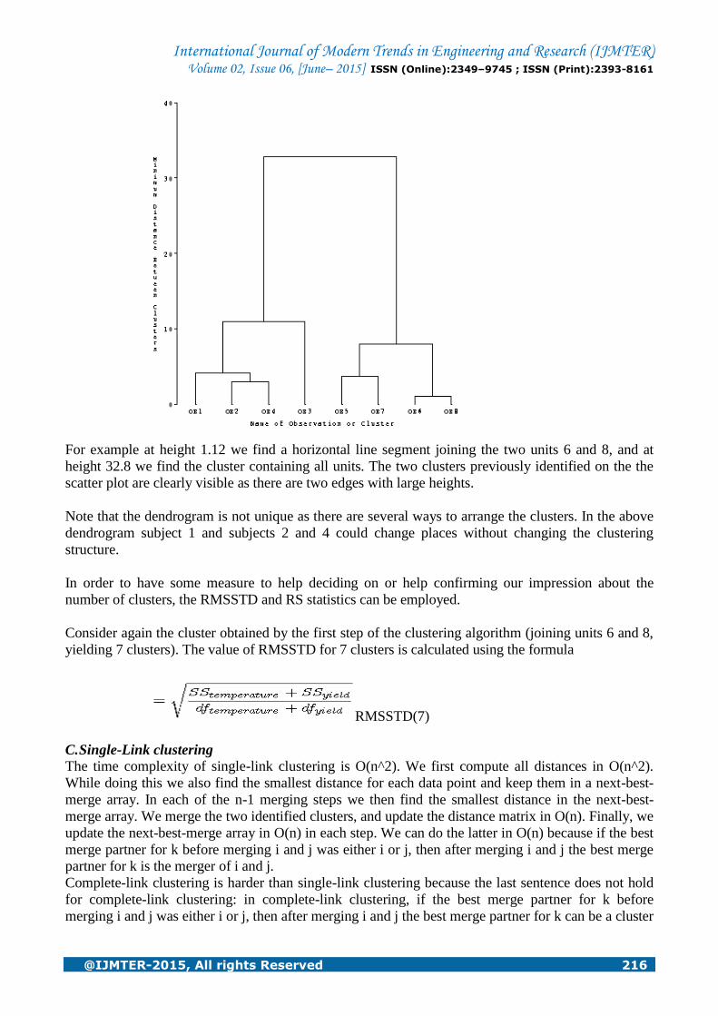
These minimum distances are the heights of the clusters in the corresponding dendrogram which is

given in Figure 2.3. The scale on the y axis is minimum distances.



For example at height 1.12 we find a horizontal line segment joining the two units 6 and 8, and at

height 32.8 we find the cluster containing all units. The two clusters previously identified on the the

scatter plot are clearly visible as there are two edges with large heights.

Note that the dendrogram is not unique as there are several ways to arrange the clusters. In the above

dendrogram subject 1 and subjects 2 and 4 could change places without changing the clustering

structure.

In order to have some measure to help deciding on or help confirming our impression about the

number of clusters, the RMSSTD and RS statistics can be employed.

Consider again the cluster obtained by the first step of the clustering algorithm (joining units 6 and 8,

yielding 7 clusters). The value of RMSSTD for 7 clusters is calculated using the formula

RMSSTD(7)

C. Single-Link clustering

The time complexity of single-link clustering is O(n^2). We first compute all distances in O(n^2).

While doing this we also find the smallest distance for each data point and keep them in a next-best-

merge array. In each of the n-1 merging steps we then find the smallest distance in the next-best-

merge array. We merge the two identified clusters, and update the distance matrix in O(n). Finally, we

update the next-best-merge array in O(n) in each step. We can do the latter in O(n) because if the best

merge partner for k before merging i and j was either i or j, then after merging i and j the best merge

partner for k is the merger of i and j.

Complete-link clustering is harder than single-link clustering because the last sentence does not hold

for complete-link clustering: in complete-link clustering, if the best merge partner for k before

merging i and j was either i or j, then after merging i and j the best merge partner for k can be a cluster



different from the merger of i and j. The reason for this difference between single-link and complete-

link is that distance defined as the distance of the two closest members is a local property that is not

affected by merging; distance defined as the diameter of a cluster is a non-local property that can

change during merging.

D. Complete-link clustering

The worst case time complexity of complete-link clustering is at most O(n^2 log n). One O(n^2 log n)

algorithm is to compute the n^2 distance metric and then sort the distances for each data point (overall

time: O(n^2 log n)). After each merge iteration, the distance metric can be updated in O(n). We pick

the next pair to merge by finding the smallest distance that is still eligible for merging. If we do this

by traversing the n sorted lists of distances, then, by the end of clustering, we will have done n^2

traversal steps. Adding all this up gives you O(n^2 log n). See also Aichholzer et al. 1996 and Day et

al. 1984. (My intuition is that complete link clustering is easier than sorting a set of n^2 numbers, so

there should be a more efficient algorithm.

E. Average-link clustering Average-link clustering merges in each iteration the pair of clusters with the highest cohesion. If our

data points are represented as normalized vectors in a Euclidean space, we can define the cohesion G

of a cluster C as the average dot product:

G(C) = 1/[n(n-1)] (gamma(C)-n)

where

n = !C!,

gamma(C) = sum(v in C) sum(w in C) <v,w>

and

<v,w> is the dot product of v and w. If we maintain an array of cluster centroids p(C), where p(C) =

[sum(v in C) v], for the currently active clusters, then gamma of the merger of C1 and C2, and hence

its cohesion, can be computed recursively as

gamma(C1+C2) = sum(v in C1+C2)sum(w in C1+C2)<v,w>

= <sum(v in C1+C2)v,sum(w in C1+C2)w>

= <p(C1+C2),p(C1+C2)>

Based on this recursive computation of cohesion, the time complexity of average-link clustering is

O(n^2 log n). We first compute all n^2 similarities for the singleton clusters, and sort them for each

cluster (time: O(n^2 log n)). In each of O(n) merge iterations, we identify the pair of clusters with the

highest cohesion in O(n); merge the pair; and update cluster centroids, gammas and cohesions of the

O(n) possible mergers of the just created cluster with the remaining clusters. For each cluster, we also

update the sorted list of merge candidates by deleting the two just merged clusters and inserting its

cohesion with the just created cluster. Each iteration thus takes O(n log n). Overall time complexity is

then O(n^2 log n).

Note that computing cluster centroids, gammas and cohesions will take time linear in the number of

unique terms T in the document collection in the worst case. In contrast, complete-link clustering is

bounded by the maximum document length D_max (if we compute similarity using the cosine for

data points represented as vectors). So complete-link clustering is O(n^2 log n D_max) whereas

average-link clustering is O(n^2 log n T). This means that we usually need to employ some form of

dimensionality reduction for efficient average-link clustering.

Also, there are only O(n^2) pairwise similarities in complete-link clustering since the similarity

between two clusters is ultimately the similarity between two vectors. In average-link clustering,

every subset of vectors can have a different cohesion, so we cannot precompute all possible cluster-

cluster similarities.



TABLE I. SUMMARY OF ALGORITHM AND THEIR PARAMETERS

Acronym Al

gor

ith

m

Attrib

utes

Dist

ance

Initial

izatio

n

K-

estima

te

Kms 100

S

K-

me

ans

100 >

TV

Cosi

ne

Rando

m

Rec.Si

l

kms 100

K-

me

ans

100>

TV

Cosi

ne

Rando

m

Simp.

Sil

Kms100*

K-

me

ans

100>

TV

Cosi

ne

Rando

m

Simp.

Sil

KmsT

100*

K-

me

ans

100>

TV

Cosi

ne

Rando

m

silhou

ette

KmsS

K-

me

ans

Cont.(

all)

Cosi

ne

Rando

m

Rec.Si

l

Kmd 100

K-

me

doi

ds

100>

TV

Cosi

ne

Rando

m

Silhou

ette

Kmd 100*

K-

me

doi

ds

100>

TV

Cosi

ne

Rando

m

Silhou

ette

Kmd Lev

K-

me

doi

ds

Name

Lev

Rando

m

Silhou

ette

Kmd Lev

S

K-

me

doi

ds

Name

Lev

Rando

m

Silhou

ette

AL 100

Av

era

ge

Lin

k

100>

TV

Cosi

ne

Rando

m

Silhou

ette

CL 100

Co

mp

lete

Lin

k

100>

TV

Cosi

ne

Rando

m

Silhou

ette



Acronym Al

gor

ith

m

Attrib

utes

Dist

ance

Initial

izatio

n

K-

estima

te

Kms 100

S

K-

me

ans

100 >

TV

Cosi

ne

Rando

m

Rec.Si

l

SL 100

Sin

gle

Lin

k

100>

TV

Cosi

ne

Rando

m

Silhou

ette

100> TV : 100 attributes (words) that have the greatest varience over the documents.

Cont.100 random :100 randomly chosen attributes from

document content.

Cont.(all): all features from document Content.

Lev : Levenshtein distance

Simp.sil : Simplified Silhouette.

Rec.Sil :”Recursive” Silhouette.

*:Initialization on distant Objects.

Name: File Name

F. Agglomerative Clustering

Agglomerative clustering can be used as long as we have pairwise distances between any two

objects. The mathematical representation of the objects are irrelevant when the pairwise distances are

given. Hence agglomerative clustering readily applies for non-vector data.

Let's denote the data set as A = {x1, ... , xn}.

The agglomerative clustering method is also called a bottom up method as opposed to k-means or k-

center methods that are top-down. In a top-down method, a data set is divided into more and more

clusters. In a bottom-up approach, all the data points are treated as individual clusters to start with

and gradually merged into bigger and bigger clusters. In agglomerative clustering clusters are

generated hierarchically. We start by taking every data point as a cluster. Then we merge two

clusters at a time. In order to decide which two clusters to merge, we compare the pairwise distances

between any two clusters and pick a pair with the minimum distance. Once we merge two clusters

into a bigger one, a new cluster is created. The distances between this new cluster and the existing

ones are not given. Some scheme has to be used to obtain these distances based on the two merged

clusters. We call this the update of distances. Various schemes of updating distances will be

described shortly. We can keep merging clusters until all the points are merged into one cluster. A

tree can be used to visualize the merging process. This tree is called dendrogram. The key technical

detail here is how we define the between-cluster distance. At the bottom level of the dendrogram

where every cluster only contains a single point, the between-cluster distance is simply the Euclidian

distance between the points, or in some applications, the between-point distances are pre-given.

However, once we merge two points into a cluster how do we get the distance between the new

cluster and the existing clusters. The idea is to somehow aggregate the distances between the objects

contained in the clusters. For clusters containing only one data point, the between-cluster distance is

the between-object distance. For clusters containing multiple data points, the between-cluster

distance is an agglomerative version of the between-object distances. There are a number of ways to

accomplish this. Examples of these aggregated distances include the minimum or maximum

between-objects distances for pairs of objects across the two clusters.

For example, suppose we have two clusters and each one has three points. One thing we could do is

to find distances between these points. In this case, there would be nine distances between pairs of



points across the two clusters. The minimum (or maximum, or average) of the nine distances can be

used as the distance between the two clusters.

How do we decide which aggregation scheme to use? Depending on how we update the distances,

dramatically different results may come up. Therefore, it is always good practice to look at the

results by scatter plots or other visualization method instead of blindly taking the output of any

algorithm. Clustering is inevitably subjective since there is no gold standard.

Normally the agglomerative between-cluster distance can be computed recursively. The aggregation

as explained above sounds computationally intensive and seemingly impractical. If we have two very

large clusters, we have to check all the between-object distances for all pairs across the two clusters.

The good news is that for many of these aggregated distances, we can update them recursively

without checking all the pairs of objects. The update approaches will be described soon.

Example Distances

Let's see how we would update between-cluster distances. Suppose we have two clusters r and s and

these two clusters, not necessarily single point clusters, are merged into a new cluster t. Let k be any

other existing cluster. We want the distance between the new cluster t had any existing cluster, k.

We will get this distance based on the distance between k and the two component clusters , r and s.

Because r and s have existed, the distance between r and k and the distance between s and k are

already computed. Denote the distances by D(r, k) and D(s, k).

We list below various ways to get D(t, k) from D(r, k) and D(s, k)?

Single-link clustering:

D(t, k) = min(D(r, k), D(s, k))

D(t, k) is the minimum distance between two objects in cluster t and k respectively. It can be shown

that the above way of updating distance is equivalent to defining the between-cluster distance as the

minimum distance between two objects across the two clusters.

Complete-link clustering:

D(t, k) = max(D(r, k), D(s, k))

Here, D(t, k) is the maximum distance between two objects in cluster t and k.

Average linkage clustering:

There are two cases here, the unweighted case and the weighted case.



Unweighted case:

Here we need to use the

number of points in

cluster r and the number

of points in cluster s, (the two clusters that are being merged together into a bigger cluster), and

compute the percentage of points in the two component clusters with respect to the merged cluster.

The two distances, D(r, k) and D(s, k), are aggregated by weighted sum.

Weighted case:

Instead of using the weight

proportional to the cluster size, we use the arithmetic mean. While this might look more like an

unweighted case, it is actually weighted in terms of the contribution from individual points in the two

clusters. When the two clusters are weighted half and half, any point (i.e., object) in the smaller

cluster individually contributes more to the aggregated distance than a point in the larger clusters. In

contrast, if the larger cluster is given proportionally higher weight, any point in either cluster

contributes equally to the aggregated distance.

Centroid clustering:

A centroid is computed for each cluster and the distance between clusters is defined as the distance

between their respective centroids.

Unweighted case:

Weighted case:

Ward's clustering:

We update the distance using the following formula:

This approach attempts to merge the two clusters for which the change in the total variation is

minimized. The total variation of a clustering result is defined as the sum of squared-error between

every object and the centroid of the cluster it belongs to. The dendrogram generated by single-linkage

clustering tends to look like a chain. Clusters generated by complete-linkage may not be well

separated. Other methods are intermediates between the two.

VI. APPLICATION

In Forensic Analysis thousands of files are usually examined. Data in those files consists of

unstructured text analyzing it by examiners is very difficult. Algorithms for clustering documents can

facilitate the discovery of new and useful knowledge from the documents under analysis. Cluster



analysis itself is not one specific algorithm but the general task to be solved. It can be achieved by

various algorithms that differ significantly in their notion of what constitutes a cluster.

Here we propose an approach that applies to clustering of

Documents seized in police investigations. Clustering has a number of applications in every field of

life. We are applying this technique whether knowingly or unknowingly in day-to-day life. One has to

cluster a lot of thing on the basis of similarity either consciously or unconsciously. Clustering is often

one of the first steps in data mining analysis. The partitioned K-means algorithm also achieved good

results when properly initialized.

Considering the approaches for estimating the number of clusters, the relative validity criterion known

as silhouette has shown to simplified version. It identifies groups of related records that can be used as

a starting point for exploring further relationships. In addition, some of our results suggest that using

the file names along with the document content in formation may be useful for cluster ensemble

algorithms. Most importantly, we observed that clustering algorithms indeed tend to induce clusters

formed by either relevant or irrelevant documents, thus contributing to enhance the expert examiner’s

job. Furthermore, our evaluation of the proposed approach in five real-world.

Data mining is used for knowledge discovering from mass data to support decision making. The

implementation aspects of applying clustering data mining method to customer analysis of department

store are studied in this paper. A data warehouse is built based on the OLTP database of Chongqing

Liangbai Department Store. Two data mining models are applied to the analysis of customer

characteristics and the relationship between customers and the product categories. The mining results

are analyzed.

Market segmentation is the telecom carrier market marketing efforts. First of all, by user

characteristics, consumption habits the breakdown of such dimensions, the general user market

segmentation will become a significant feature of a number of market segments, so that the same fine

between the individual sub-markets to minimize the inherent differences make the difference between

the different market segments to the most great, then you can combine features of different market

segments to develop specific strategies to effectively develop and meet specific market and consumer

demand. So far, this article has introduced the two clustering methods: Q-type factor clustering and

correspondence analysis clustering method. We can see that the two methods in terms of ideology or

in the algorithm, there are a lot of similarities. For instance,

both methods are time complexity of the sample size of the linear stage, two kinds of methods to Q-

Factor load matrix for clustering based on factor scores are used to explain features of the category,

and so on. Of course, both methods have some obvious differences:

(1). although the two methods in Q-factor loading matrix as a cluster basis, but the measure of both

space is not like Q-factor clustering method is based on European metric space, while the

corresponding analysis of clustering.

(2). Secondly, although both methods are low by solving a matrix of characteristic roots and

characteristic vectors and thus inter- ground by Q-factor loading matrix of ways to improve the

efficiency.

(3). Finally, Q-type factor analysis clustering method can only be applied to quantitative data analysis,

and the corresponding analysis not only can deal with quantitative data, qualitative data can deal with.

VII. CONCLUSION

Clustering and classification are both fundamental tasks in Data Mining. Classification is used

mostly as a supervised learning method, clustering for unsupervised learning (some clustering

models are for both). The goal of clustering is descriptive, that of classification is predictive

(Veyssieres and Plant,1998). Since the goal of clustering is to discover a new set of categories, the

new groups are of interest in themselves, and their assessment is intrinsic. In classification tasks,

however, an important part of the assessment is extrinsic,since the groups must reflect some

reference set of classes.

“Understanding our world requires conceptualizing the similarities and differences between the



entities that compose it”

ACKNOWLEDGMENT

The preferred spelling of the word “acknowledgment” in America is without an “e” after the “g”.

Avoid the stilted expression, “One of us (R. B. G.) thanks . . .” Instead, try

“R. B. G. thanks”. Put applicable sponsor acknowledgments here; DO NOT place them on the first

page of your paper or as a footnote.

REFERENCES [1] G.C. Oatley, J. Zeleznikow, B.W. Ewart, ‘Matching and Predicting Crimes,’ In Applications and Innovations in

Intelligent Systems XII in Proceedings of AI2004, The Twenty-fourth SGAI International Conference on Knowledge

Based Systems and Applications of Artificial Intelligence. Ann Macintosh, Richard Ellis and Tony Allen Ed. London:

Springer,, pp. 19–32, 2004.

[2] R. William Adderley, ‘The use of data mining techniques in crime trend analysis and offender profiling,’ Ph.D. thesis,

University of Wolverhampton, Wolverhampton, England, 2007.

[3] Y. Xiang, M. Chau, H. Atabakhsh, H. Chen Visualizing criminal relationships: comparison of a hyperbolic tree and a

hierarchical list Decision support systems, Elsevier Science Publishers, 41 (1) (2005), pp. 69–83

[4] Chen W. Chung, Y. Qin, M. Chau, J. Xu, G. Wang, R. Zheng, H. Atabakhsh, ‘Crime Data Mining: An Overview and

Case Studies,’ in Proceedings of the 3rd National Conference for Digital Government Research (dg.o 2003), pp. 1-5,

Boston, MA, May 18-21, 2003.

[5] H. Chen, H. Atabakhsh, T. Petersen, J. Schroeder, T. Buetow, L. Chaboya, C. O’Toole, M. Chau, T. Cushna, D. Casey,

Z. Huang, ‘COPLINK: Visualization for Crime Analysis,’ ACM International Conference Proceeding Series, Proceedings

of the 2003 annual national conference on digital government research,, Vol. 130, pp 1-6, Boston, MA, 2003.

[6] R.V. Hauck, H. Atabakhsh, P. Ongvasith, H. Gupta, H. Chen Using Coplink to Analyze Criminal-Justice Data

Computer, 35 (3) (2002), pp. 30–37

[7] H. Chen, W. Chung, J.J Xu, G. Wang, Y. Qin, M. Chau Crime data mining: A general framework and some examples

Computer, 37 (4) (2004), pp. 50–56

[8]J. Han, M. Kamber Data Mining Concepts and Techniques (2nd edn)Morgan Kaufmann (2005)

[9]D.J. Hand, H. Mannila, P. Smyth Principles of Data MiningMIT Press, Massachusetts (2001)

[10]G.K. Gupta Introduction to Data Mining with Case StudiesPrentice-hall of India, New Delhi (2006)