Department of Computer Science 6 King’s College Rd, TorontoUniversity of Toronto M5S 3G4, Canadahttp://learning.cs.toronto.edu fax: +1 416 978 1455

Copyright c© Geoffrey Hinton 2006.

October 26, 2006

UTML TR 2006–004

To Recognize Shapes, First

Learn to Generate Images

Geoffrey Hinton

Department of Computer Science, University ofToronto

To Recognize Shapes, First Learn to Generate Images

Geoffrey HintonDepartment of Computer Science

University of Toronto&

Canadian Institute for Advanced Research

October 26, 2006

The uniformity of the cortical architecture and the ability of functions to move todifferent areas of cortex following early damage strongly suggests that there is a singlebasic learning algorithm for extracting underlying structure from richly-structured, high-dimensional sensory data. There have been many attempts to design such an algorithm,but until recently they all suffered from serious computational weaknesses. This chapterdescribes several of the proposed algorithms and shows how they can be combined toproduce hybrid methods that work efficiently in networks with many layers and millionsof adaptive connections.

Five strategies for learning multilayer networks

Half a century ago, Oliver Selfridge (Selfridge, 1958) proposed a pattern recognitionsystem called “Pandemonium” consisting of multiple layers of feature detectors. Hisactual proposal contained a considerable amount of detail about what each of the layerswould compute but the basic idea was that each feature detector would be activatedby some familiar pattern of firing among the feature detectors in the layer below. Thiswould allow the layers to extract more and more complicated features culminating in a toplayer of detectors that would fire if and only if a familiar object was present in the visualinput. Over the next 25 years, many attempts were made to find a learning algorithmthat would be capable of discovering appropriate connection strengths (weights) for thefeature detectors in every layer. Learning the weights of a single feature detector isquite easy if we are given both the inputs to the feature detector and its desired firingbehaviour, but learning is much more difficult if we are not told how the intermediatelayers of feature detectors ought to behave. These intermediate feature detectors arecalled “hidden units” because their desired states cannot be observed. There are severalstrategies for learning the incoming weights of the hidden units.

The first strategy is denial. If we assume that there is only one layer of hidden units,it is often possible to set their incoming weights by hand using domain-specific knowl-edge. So the problem of learning hidden units does not exist. Within neuroscience, the

2

equivalent of using hand-coded features is to assume that the receptive fields of featuredetectors are specified innately – a view that is increasingly untenable (Merzenich et al.,1983; Sharma et al., 2000; Karni et al., 1994). Most of the work on perceptrons (Rosen-blatt, 1962; Minsky and Papert, 1969) used hand-coded feature detectors, so learningonly occurred for the weights from the feature detectors to the final decision units whosedesired states were known. To be fair to Rosenblatt, he was well aware of the limitationsof this approach – he just didn’t know how to learn multiple layers of features efficiently.The current version of denial is called “support vector machines” (Vapnik, 2000). Thesecome with a fixed, non-adaptive recipe for converting a whole training image into afeature and a clever optimization technique for deciding which training cases should beturned into features and how these features should be weighted. Their main attractionis that the optimization method is guaranteed to find the global minimum. They areinadequate for tasks like 3-D object recognition that cannot be solved efficiently using asingle layer of feature detectors (LeCun et al., 2004) but they work undeniably well formany of the simpler tasks that are used to evaluate machine learning algorithms (Decosteand Schoelkopf, 2002).

The second strategy is based on an analogy with evolution – randomly jitter theweights and save the changes that cause the performance of the whole network to improve.This is attractive because it is easy to understand, easy to implement in hardware (Jabriand Flower, 1992), and it works for almost any type of network. But it is hopelesslyinefficient when the number of weights is large. Even if we only change one weight ata time, we still have to classify a large number of images to see if that single changehelps or hurts. Changing many weights at the same time is no more efficient becausethe changes in other weights create noise that prevents each weight from detecting whateffect it has on the overall performance. The evolutionary strategy can be significantlyimproved by applying the jitter to the activities of the feature detectors rather than tothe weights (Mazzoni et al., 1991; Seung, 2003), but it is still an extremely inefficient wayto discover gradients. Even blind evolution must have stumbled across a better strategythan this.

The third strategy is procrastination. Instead of learning feature detectors that aredesigned to be helpful in solving the classification problem, we can learn a layer offeature detectors that capture interesting regularities in the input images and put off theclassification problem until later. This strategy can be applied recursively: We can learna second layer of feature detectors that capture interesting regularities in the patternsof activation of the first layer detectors, and so on for as many layers as we like. Thehope is that the features in the higher layers will be much more useful for classificationthan the raw inputs or the features in lower layers. As we shall see, this is not justwishful thinking. The main difficulties with the layer-by-layer strategy are that we needa quantitative definition of what it means for a regularity to be “interesting” and we needa way of ensuring that different feature detectors within a layer learn to detect differentregularities even if they receive the same inputs.

The fourth strategy is to use calculus. To apply this strategy we need the output ofeach hidden unit to be a smooth function of the inputs it receives from the layer below.We also need a cost function that measures how poorly the network is performing. Thiscost function must change smoothly with the weights, so the number of classificationerrors is not the right function. For classification tasks, we can interpret the outputs

3

of the top-level units as class probabilities and an appropriate cost function is then thecross-entropy which is the negative log probability that the network assigns to the correctclass. Given appropriate hidden units and an appropriate cost function, the chain rulecan be used to compute how the cross-entropy changes as each weight in the networkis changed. This computation can be made very efficient by first computing, for eachhidden unit, how the cross-entropy changes as the activity of that hidden unit is changed.This is known as backpropagation because the computation starts at the output layerand proceeds backwards through the network one layer at a time. Once we know howthe activity of a hidden unit affects the cross-entropy on each training case we have asurrogate for the desired state of the hidden unit and it is easy to change the incomingweights to decrease the sum of the cross-entropies on all the training cases. Comparedwith random jittering of the weights or feature activations, backpropagation is moreefficient by a factor of the number of weights or features in the network.

Backpropagation was discovered independently by several different researchers (Brysonand Ho, 1975; Werbos, 1974; Parker, 1985; LeCun, 1985; Rumelhart et al., 1986) and itwas the first effective way to learn neural networks that had one or more layers of adaptivehidden units. It works very well for tasks such as the recognition of handwritten digits(LeCun et al., 1998; Simard et al., 2003), but it has two serious computational problemsthat will be addressed in this chapter. First, it is necessary to choose initial randomvalues for all the weights. If these values are small, it is very difficult to learn deep net-works because the gradients decrease multiplicatively as we backpropagate through eachhidden layer. If the initial values are large, we have randomly chosen a particular regionof the weight-space and we may well become trapped in a poor local optimum withinthis region. Second, the amount of information that each training case provides aboutthe mapping between images and classes is at most the log of the number of possibleclasses. This means that large networks require a large amount of labeled training dataif they are to learn weights that generalize well to novel test cases.

Many neuroscientists treat backpropagation with deep suspicion because it is not atall obvious how to implement it in cortex. In particular, it is hard to see how a singleneuron can communicate both its activity and the deriviative of the cost function withrespect to its activity. It seems very unlikely, however, that hundreds of millions of yearsof evolution have failed to find an effective way of tuning lower-level feature detectors sothat they provide the outputs that higher-level detectors need in order to make the rightdecision.

The fifth and last strategy in this survey was designed to allow higher-level featuredetectors to communicate their needs to lower-level ones whilst also being easy to im-plement in layered networks of stochastic, binary neurons that have activation states of1 or 0 and turn on with a probability that is a smooth non-linear function of the totalinput they receive:

p(sj = 1) =1

1 + exp(−bj −∑

i siwij)(1)

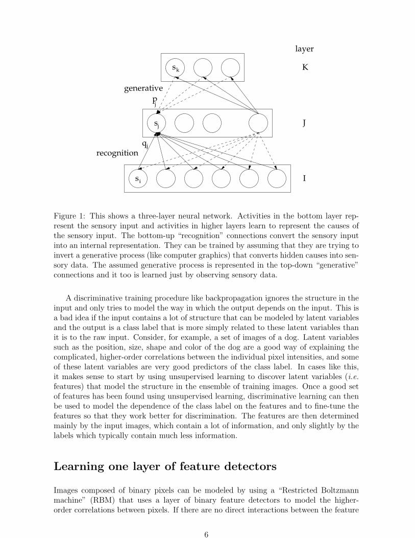
where si and sj are the binary activities of units i and j, wij is the weight on theconnection from i to j, and bj is the bias of unit j. Imagine that the training datawas generated top-down by a multilayer “graphics” model of the type shown in figure1. The binary state of a hidden unit that was actually used to generate an image top-down could then be used as its desired state when learning the bottom-up “recognition”

4

weights. At first sight, this idea of using top-down “generative” connections to providedesired states for the hidden units does not appear to help because we now have to learna graphics model that can generate the training data. If, however, we already had somegood recognition connections we could use a bottom-up pass from the real training datato activate the units in every layer and then we could learn the generative weights bytrying to reconstruct the activities in each layer from the activities in the layer above.So we have a chicken-and-egg problem: Given the generative weights we can learn therecognition weights and given the recognition weights we can learn the generative weights.It turns out that we can learn both sets of weights by starting with small random valuesand alternating between two phases of learning. In the “wake” phase, the recognitionweights are used to drive the units bottom-up, and the binary states of units in adjacentlayers can then be used to train the generative weights. In the “sleep” phase, the top-down generative connections are used to drive the network, so it produces fantasies fromits generative model. The binary states of units in adjacent layers can then be used tolearn the bottom-up recognition connections (Hinton et al., 1995). The learning rules arevery simple. During the wake phase, a generative weight, gkj, is changed by

∆gkj = εsk(sj − pj) (2)

where unit k is in the layer above unit j, ε is a learning rate and pj is the probabilitythat unit j would turn on if it were being driven by the current states of the units in thelayer above using the current generative weights. During the sleep phase, a recognitionweight, wij, is changed by

∆wij = εsi(sj − qj) (3)

where qj is the probability that unit j would turn on if it were being driven by the currentstates of the units in the layer below using the current recognition weights.

The rest of this chapter shows that the performance of both backpropagation (strategyfour) and the “wake-sleep” algorithm (strategy five) can be greatly improved by using a“pre-training” phase in which unsupervised layer-by-layer learning is used to make thehidden units in each layer represent regularities in the patterns of activity of units inthe layer below (strategy three). With this type of pretraining, it is finally possible tolearn deep, multilayer networks efficiently and to demonstrate that they are better atclassification than shallow methods.

Learning feature detectors with no supervision

Classification of isolated, normalized shapes like those shown in figure 2 has been one ofthe paradigm tasks for demonstrating the pattern recognition abilities of artificial neuralnetworks. The connection weights in a multi-layer network are typically initialized byusing small random values which are then iteratively adjusted by backpropagating thedifference between the desired output of the network on each training case and the outputthat it actually produces on that training case. To prevent the network from modelingaccidental regularities that arise from the random selection of training examples, it iscommon to stop the training early or to impose a penalty on large connection weights.This improves the final performance of the network on a test set, but it is not nearly aseffective as using a more intelligent strategy for initializing the weights.

5

pj

sj

si

s

qj

generative

layer

K

J

I

recognition

k

Figure 1: This shows a three-layer neural network. Activities in the bottom layer rep-resent the sensory input and activities in higher layers learn to represent the causes ofthe sensory input. The bottom-up “recognition” connections convert the sensory inputinto an internal representation. They can be trained by assuming that they are trying toinvert a generative process (like computer graphics) that converts hidden causes into sen-sory data. The assumed generative process is represented in the top-down “generative”connections and it too is learned just by observing sensory data.

A discriminative training procedure like backpropagation ignores the structure in theinput and only tries to model the way in which the output depends on the input. This isa bad idea if the input contains a lot of structure that can be modeled by latent variablesand the output is a class label that is more simply related to these latent variables thanit is to the raw input. Consider, for example, a set of images of a dog. Latent variablessuch as the position, size, shape and color of the dog are a good way of explaining thecomplicated, higher-order correlations between the individual pixel intensities, and someof these latent variables are very good predictors of the class label. In cases like this,it makes sense to start by using unsupervised learning to discover latent variables (i.e.features) that model the structure in the ensemble of training images. Once a good setof features has been found using unsupervised learning, discriminative learning can thenbe used to model the dependence of the class label on the features and to fine-tune thefeatures so that they work better for discrimination. The features are then determinedmainly by the input images, which contain a lot of information, and only slightly by thelabels which typically contain much less information.

Learning one layer of feature detectors

Images composed of binary pixels can be modeled by using a “Restricted Boltzmannmachine” (RBM) that uses a layer of binary feature detectors to model the higher-order correlations between pixels. If there are no direct interactions between the feature

6

Figure 2: Some examples of real handwritten digits that are hard to recognize. A neuralnetwork described at the end of this chapter gets all of these examples right, even thoughit has never seen them before. However, it is not confident about its classification forany of these examples. The true classes are arranged in standard scan order.

detectors and no direct interactions between the pixels, there is a simple and efficientway to learn a good set of feature detectors from a set of training images (Hinton, 2002).We start with zero weights on the symmetric connections between each pixel i and eachfeature detector j. Then we repeatedly update each weight, wij, using the differencebetween two measured, pairwise correlations

∆wij = ε(<sisj>data − <sisj>recon) (4)

where ε is a learning rate, < sisj >data is the frequency with which pixel i and featuredetector j are on together when the feature detectors are being driven by images from thetraining set and <sisj>recon is the corresponding frequency when the feature detectorsare being driven by reconstructed images. A similar learning rule can be use dfor thebiases.

Given a training image, we set the binary state, sj, of each feature detector to be 1with probability

p(sj = 1) =1

1 + exp(−bj −∑

i∈pixels siwij)(5)

where bj is the bias of j and si is the binary state of pixel i. Once binary states havebeen chosen for the hidden units we produce a “reconstruction” of the training image bysetting the state of each pixel to be 1 with probability

p(si = 1) =1

1 + exp(−bi −∑

j∈features sjwij)(6)

On 28 × 28 pixel images of handwritten digits like those shown in figure 2, goodfeatures can be found by using 100 passes through a training set of 50,000 images, with

7

Figure 3: The receptive fields of some feature detectors. Each gray square shows theincoming weights to one feature detector from all the pixels. Pure white means a positiveweight of at least 3 and pure black means a negative weight of at least −3. Most of thefeature detectors learn highly localized receptive fields.

the weights being updated after every 100 images using the pixel-feature correlationsmeasured on selected subset of the features that are learned. Some features have anon-center off-surround structure (or the reverse) and these are a good way to model thesimple fact that if a pixel is on, nearby pixels tend to be on. Some features detect parts ofstrokes, and they typically inhibit the region of the image that is further from the centerthan the stroke fragment. Some features, which look more like fingerprints, encode thephase and amplitude of high-frequency fourier components of a large part of the wholeimage. These features tend to turn on about half the time and can be eliminated byforcing features to only turn on rarely (Ranzato et al., 2007). The three features withunnaturally sharp black lines capture the fact that if a pixel is on, pixels that are morethan 20 rows above or below it cannot be on because of the way the data was normalized.

The learned weights and biases of the features implicitly define a probability distri-bution over all possible binary images. Sampling from this distribution is difficult, but itcan be done by using “alternating Gibbs sampling”. This starts with a random image andthen alternates between updating all of the features in parallel using Eq. 5 and updatingall of the pixels in parallel using Eq. 6. After Gibbs sampling for sufficiently long, thenetwork reaches “thermal equilibrium”. The states of pixels and features detectors stillchange, but the probability of finding the system in any particular binary configurationdoes not.

8

A greedy learning algorithm for multiple hidden layers

A single layer of binary features is not the best way to model the structure in a set ofimages. After learning the first layer of feature detectors, a second layer can be learnedin just the same way by treating the existing feature detectors, when they are beingdriven by training images, as if they were data. To reduce noise in the learning signal,the binary states of feature detectors (or pixels) in the “data” layer are replaced by theirreal-valued probabilities of activation when learning the next layer of feature detectors,but the new feature detectors have binary states to limit the amount of informationthey can convey. This greedy, layer-by-layer learning can be repeated as many times asdesired. To justify this layer-by-layer approach, it would be good to show that adding anextra layer of feature detectors always increases the probability that the overall generativemodel would generate the training data. This is almost true: Provided the number offeature detectors does not decrease and their weights are initialized correctly, adding anextra layer is guaranteed to raise a lower bound on the log probability of the trainingdata (Hinton et al., 2006). So after learning several layers there is good reason to believethat the feature detectors will have captured many of the statistical regularities in theset of training images and we can now test the hypothesis that these feature detectorswill be useful for classification.

Using backpropagation for discriminative fine-tuning

After greedily learning layers of 500, 500, and 2000 feature detectors without using anyinformation about the class labels, gentle backpropagation was used to fine-tune theweights for discrimination. This produced much better classification performance on testdata than using backpropagation without the initial, unsupervised phase of learning.The MNIST data set used for these experiments has been used as a benchmark for manyyears and many different researchers have tried using many different learning methods,including variations of backpropagation in nets with different numbers of hidden layersand different numbers of hidden units per layer.

There are several different versions of the MNIST learning task. In the most difficultversion, the learning algorithm is not given any prior knowledge of the geometry of imagesand it is forbidden to increase the size of the training set by using small affine or elasticdistortions of the training images. Consequently, if the same random permutation isapplied to the pixels of every training and test image, the performance of the learningalgorithm will be unaffected. For this reason, this is called the “permutation invariant”version of the task. So far as the learning algorithm is concerned, each 28×28 pixel imageis just a vector of 784 numbers that has to be given one of 10 labels. The best publishedbackpropagation error rate for this version of the task is 1.6% (Platt et. al.). Supportvector machines can achieve 1.4% (Decoste and Schoelkopf, 2002). Table 1 shows thatthe error rate of backpropagation can be reduced to about 1.12% if it is only used forfine-tuning features that are originally discovered by layer-by-layer pretraining.

9

Details of the discriminative fine-tuning procedure

Using three different splits of the 60,000 image training set into 50,000 training examplesand 10,000 validation examples, the greedy learning algorithm was used to initialize theweights and biases and gentle backpropagation was then used to fine-tune the weights.After each sweep through the training set (which is called an “epoch”), the classificationerror rate was measured on the validation set. Training was continued until two condi-tions were satisfied. The first condition involved the average cross-entropy error on thevalidation set. This is the quantity that is being minimized by the learning algorithmso it always falls on the training data. On the validation data, however, it starts risingas soon as overfitting occurs. There is strong tendency for the number of classificationerrors to continue to fall after the cross-entropy has bottomed-out on the validation data,so the first condition is that the learning must have already gone past the minimum ofthe cross-entropy on the validation set. It is easy to detect when this condition is sat-isfied because the cross-entropy changes very smoothly during the learning. The secondcondition involved the number of errors on the validation set. This quantity fluctuatesunpredictably, so the criterion was that the minimum value observed so far should haveoccurred at least 10 epochs ago. Once both conditions were satisfied, the weights andbiases were restored to the values they had when the number of validation set errorswas at its minimum, and performance on the 10,000 test cases was measured. As shownin table 1, this gave test error rates of 1.22% 1.16% and 1.24% on the three differentsplits. The fourth line of the table shows that these error rates can be reduced to 1.10%by multiplying together the three probabilities that the three nets predict for each digitclass and picking the class with the maximum product.

Once the performance on the validation set has been used to find a good set of weights,the cross-entropy error on the training set is recorded. Performance on the test data canthen be further improved by adding the validation set to the training set and continuingthe training until the cross-entropy on the expanded training set has fallen to the valueit had on the original training set for the weights selected by the validation procedure.As shown in table 1 this eliminates about 8% of the errors. Combining the predictionsof all three models produces less improvement than before because each model has nowseen all of the training data. The final line of table 1 shows that backpropagation in thisrelatively large network gives much worse results if no pretraining is used. For this lastexperiment, the stopping criterion was set to be the average of the stopping criteria fromthe previous experiments.

To avoid making large changes to the weights found by the pretraining, the back-propagation stage of learning used a very small learning rate which made it very slow,so a new trick was introduced which sped up the learning by about a factor of three.Most of the computational effort is expended computing the almost non-existent gra-dients for “easy” training cases that the network can already classify confidently andcorrectly. It is tempting to make a note of these easy cases and then just ignore them,checking every few epochs to see if the cross-entropy error on any of the ignored cases hasbecome significant. This can be done without changing the expected value of the overallgradient by using a method called importance sampling. Instead of being completelyignored, easy cases are selected with a probability of 0.1, but when they are selected, thecomputed gradients are multiplied by 10. Using more extreme values like 0.01 and 100is dangerous because a case that used to be easy might have developed a large gradient

10

pre- backprop train train train valid. valid. test testtrained training epochs cost errs cost errs cost errsnetwork set size per 100 per 100 per 100Neta 50,000 33 0.12 1 6.49 129 6.22 122Netb 50,000 56 0.04 0 7.81 118 6.21 116Netc 50,000 63 0.03 0 8.12 118 6.73 124Combined 5.75 110Neta 60,000 33+16 <0.12 1 5.81 113Netb 60,000 56+28 <0.04 0 5.90 106Netc 60,000 63+31 <0.03 0 5.93 118Combined 5.40 106not pre-pretrained 60,000 119 <0.063 0 18.43 227

Table 1: Neta, Netb, and Netc were greedily pretrained on different, unlabeled, subsets ofthe training data that were obtained by removing disjoint validation sets of 10,000 images.After pretraining, they were trained on those same subsets using backpropagation. Thenthe training was continued on the full training set until the cross-entropy error reachedthe criterion explained in the text.

while it was being ignored, and multiplying this gradient by 100 could give the networka shock. When using importance sampling, an “epoch” was redefined to be the time ittakes to sample as many training cases as the total number in the training set. So anepoch typically involves several sweeps through the whole set of training examples, butit is the same amount of computation as one sweep without importance sampling.

After the results in table 1 were obtained using the rather complicated version ofbackpropagation described above, Ruslan Salakhutdinov discovered that similar resultscan be obtained using a standard method called “conjugate gradient” which takes thegradients delivered by backpropagation and uses them in a more intelligent way thansimply changing each weight in proportion to its gradient (Hinton and Salakhutdi-nov, 2006). The MNIST data together with the Matlab code required for pretrainingand fine-tuning the network are available at http://www.cs.toronto.edu/~hinton/

MatlabForSciencePaper.html.

Using extra unlabeled data

Since the greedy pretraining algorithm does not require any labeled data, it should be avery effective way to make use of unlabeled examples to improve performance on a smalllabeled dataset. Learning with only a few labeled examples is much more characteristicof human learning. We see many instances of many different types of object, but we arevery rarely told the name of an object. Preliminary experiments confirm that pretrainingon unlabeled data helps a lot, but for a proper comparison it will be necessary to usenetworks of the appropriate size. When the number of labeled examples is small, itis unfair to compare the performance of a large network that makes use of unlabeled

11

examples with a network of the same size that does not make use of the unlabeledexamples.

Using geometric prior knowledge

The greedy pretraining improves the error rate of backpropagation by about the sameamount as methods that make use of prior knowledge about the geometry of images, suchas weight-sharing (LeCun et al., 1998) or enlarging the training set by using small affine orelastic distortions of the training images. But pretraining can also be combined with theseother methods. If translations of up to 2 pixels are used to create 12 extra versions of eachtraining image, the error rate of the best support vector machine falls from 1.4% to 0.56%(Decoste and Schoelkopf, 2002). The average error rate of the pretrained neural net fallsfrom 1.12% to 0.65%. The translated data is presumably less helpful to the multilayerneural net because the pretraining can already capture some of the geometrical structureeven without the translations. The best published result for a single method is currently0.4%, which was obtained using backpropagation in a multilayer neural net that usesboth weight-sharing and sophisticated, elastic distortions (Simard et al., 2003). The ideaof using unsupervised pretraining to improve the performance of backpropagation hasrecently been applied to networks that use weight-sharing and it consistently reduces theerror rate by about 0.1% even when the error rate is already very low (Ranzato et al.,2007).

Using contrastive wake-sleep for generative fine-tuning

Figure 4 shows a multilayer generative model in which the top two layers interact viaundirected connections and form an associative memory. At the start of learning, allconfigurations of this top-level associative memory have roughly equal energy. Learningsculpts the energy landscape and after learning the associative memory will settle intolow-energy states that represent images of digits. Valleys in the high-dimensional energy-landscape represent digit classes. Directions along the valley floor represent the allowablevariations of a digit and directions up the side of a valley represent implausible variationsthat make the image surprising to the network. Turning on one of the 10 label unitslowers one whole valley and raises the other valleys. The number of valleys and thedimensionality of each valley floor are determined by the the set of training examples.

The states of the associative memory are just binary activity vectors that look nothinglike the images they represent, but it is easy to see what the associative memory has inmind. First, the 500 hidden units that form part of the associative memory are used tostochastically activate some of the units in the layer below via the top-down, generativeconnections. Then these activated units are used to provide top-down input to thepixels. Figure 5 shows some fantasies produced by the trained network when the top-level associative memory is allowed to wander stochastically between low-energy states,but with one of the label units clamped so that it tends to stay in the same valley. Thefact that it can generate a wide variety of slightly implausible versions of each type ofdigit makes it very good at recognizing poorly written digits. A demonstration thatshows the network generating and recognizing digit images is available at http://www.

12

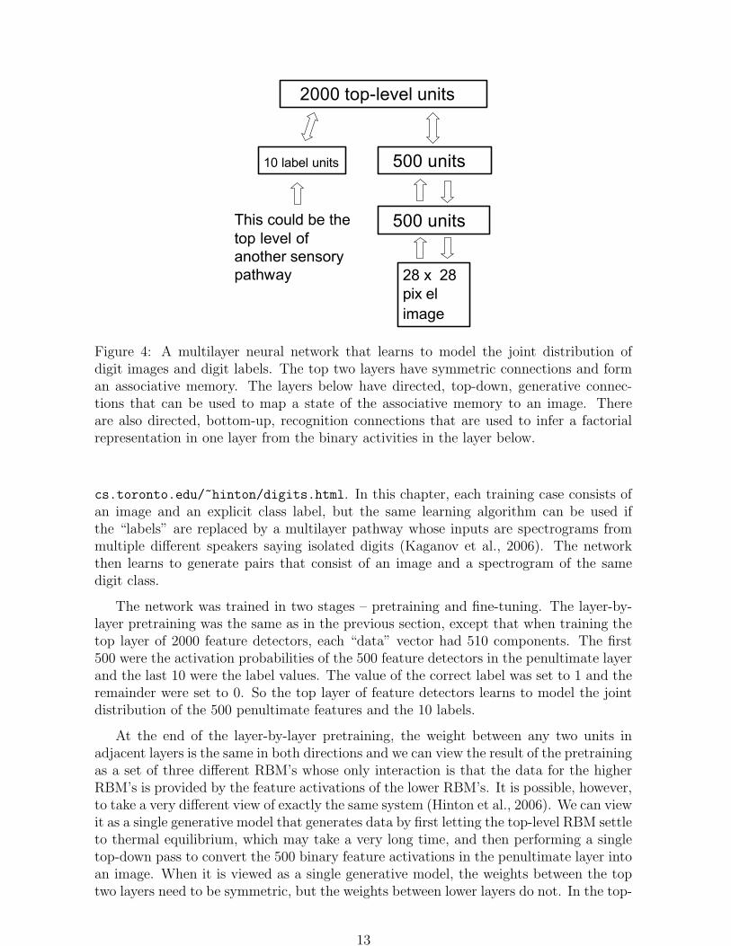
2000 top-level units

500 units

500 units

28 x 28

pixel

image

10 label units

This could be the

top level of

another sensory

pathway

Figure 4: A multilayer neural network that learns to model the joint distribution ofdigit images and digit labels. The top two layers have symmetric connections and forman associative memory. The layers below have directed, top-down, generative connec-tions that can be used to map a state of the associative memory to an image. Thereare also directed, bottom-up, recognition connections that are used to infer a factorialrepresentation in one layer from the binary activities in the layer below.

cs.toronto.edu/~hinton/digits.html. In this chapter, each training case consists ofan image and an explicit class label, but the same learning algorithm can be used ifthe “labels” are replaced by a multilayer pathway whose inputs are spectrograms frommultiple different speakers saying isolated digits (Kaganov et al., 2006). The networkthen learns to generate pairs that consist of an image and a spectrogram of the samedigit class.

The network was trained in two stages – pretraining and fine-tuning. The layer-by-layer pretraining was the same as in the previous section, except that when training thetop layer of 2000 feature detectors, each “data” vector had 510 components. The first500 were the activation probabilities of the 500 feature detectors in the penultimate layerand the last 10 were the label values. The value of the correct label was set to 1 and theremainder were set to 0. So the top layer of feature detectors learns to model the jointdistribution of the 500 penultimate features and the 10 labels.

At the end of the layer-by-layer pretraining, the weight between any two units inadjacent layers is the same in both directions and we can view the result of the pretrainingas a set of three different RBM’s whose only interaction is that the data for the higherRBM’s is provided by the feature activations of the lower RBM’s. It is possible, however,to take a very different view of exactly the same system (Hinton et al., 2006). We can viewit as a single generative model that generates data by first letting the top-level RBM settleto thermal equilibrium, which may take a very long time, and then performing a singletop-down pass to convert the 500 binary feature activations in the penultimate layer intoan image. When it is viewed as a single generative model, the weights between the toptwo layers need to be symmetric, but the weights between lower layers do not. In the top-

13

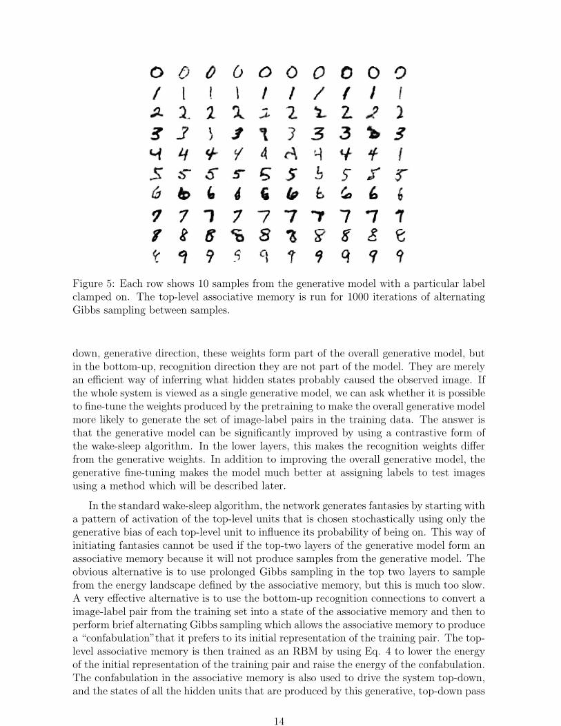
Figure 5: Each row shows 10 samples from the generative model with a particular labelclamped on. The top-level associative memory is run for 1000 iterations of alternatingGibbs sampling between samples.

down, generative direction, these weights form part of the overall generative model, butin the bottom-up, recognition direction they are not part of the model. They are merelyan efficient way of inferring what hidden states probably caused the observed image. Ifthe whole system is viewed as a single generative model, we can ask whether it is possibleto fine-tune the weights produced by the pretraining to make the overall generative modelmore likely to generate the set of image-label pairs in the training data. The answer isthat the generative model can be significantly improved by using a contrastive form ofthe wake-sleep algorithm. In the lower layers, this makes the recognition weights differfrom the generative weights. In addition to improving the overall generative model, thegenerative fine-tuning makes the model much better at assigning labels to test imagesusing a method which will be described later.

In the standard wake-sleep algorithm, the network generates fantasies by starting witha pattern of activation of the top-level units that is chosen stochastically using only thegenerative bias of each top-level unit to influence its probability of being on. This way ofinitiating fantasies cannot be used if the top-two layers of the generative model form anassociative memory because it will not produce samples from the generative model. Theobvious alternative is to use prolonged Gibbs sampling in the top two layers to samplefrom the energy landscape defined by the associative memory, but this is much too slow.A very effective alternative is to use the bottom-up recognition connections to convert aimage-label pair from the training set into a state of the associative memory and then toperform brief alternating Gibbs sampling which allows the associative memory to producea “confabulation”that it prefers to its initial representation of the training pair. The top-level associative memory is then trained as an RBM by using Eq. 4 to lower the energyof the initial representation of the training pair and raise the energy of the confabulation.The confabulation in the associative memory is also used to drive the system top-down,and the states of all the hidden units that are produced by this generative, top-down pass

14

are used as targets to train the bottom-up recognition connections. The “wake” phase isjust the same as in the standard wake-sleep algorithm: After the initial bottom-up pass,the top-down, generative connections in the bottom two layers are trained, using Eq. 2,to reconstruct the activities in the layer below from the activities in the layer above. Thedetails are given in (Hinton et al., 2006).

Fine-tuning with the contrastive wake-sleep algorithm is about an order of magnitudeslower than fine-tuning with backpropagation, partly because it has a more ambitiousgoal. The network shown in figure 4 takes a week to train on a 3GHz machine. Theexamples shown in figure 2 were all classified correctly by this network which gets atest error rate of 1.25%. This is slightly worse than pretrained networks with the samearchitecture that are fine-tuned with backpropagation, but it is better than the 1.4%achieved by the best support vector machine on the permutation-invariant version of theMNIST task. It is rare for a generative model to outperform a good discriminative modelat discrimination.

There are several different ways of using the generative model for discrimination. Iftime was not an issue, it would be possible to use sampling methods to measure therelative probabilities of generating each of the ten image-label pairs that are obtained bypairing the test image with each of the 10 possible labels. A fast and accurate approx-imation can be obtained by first performing a bottom-up pass in which the activationprobabilities of the first layer of hidden units are used to compute activation probabilitiesfor the penultimate hidden layer. Using probabilities rather than stochastic binary statessuppresses the noise due to sampling. Then the vector of activation probabilities of thefeature detectors in the penultimate layer is paired with each of the ten labels in turnand the “free energy” of the associative memory is computed. Each of the top-level unitscontributes additively to this free energy, so it is easy to calculate exactly (Hinton et al.,2006). The label that gives the lowest free-energy is the network’s guess.

Fitting a generative model constrains the weights of the network far more stronglythan fitting a discriminative model, but if the ultimate objective is discrimination, italso wastes a lot of the discriminative capacity. This waste shows up in the fact thatafter fine-tuning the generative model, its discriminative performance on the trainingdata is about the same as its discriminative performance on the test data – there isalmost no overfitting. This suggests one final experiment. After first using contrastivewake-sleep for fine-tuning, further fine-tuning can be performed using a weighted averageof the gradients computed by backpropagation and by contrastive wake-sleep. Using avalidation set, the coefficient controlling the contribution of the backpropagation gradientto the weighted average was gradually increased to find the coefficient value at which theerror rate on the validation set was minimized. Using this value of the coefficient, the testerror rate was 0.97% which is the current record for the permutation-invariant MNISTtask. It is also possible to combine the gradient from backpropagation with the gradientcomputed by the pretraining (Bengio et al., 2006). This is much less computational effortthan using contrastive wake-sleep, but does not perform as well.

AcknowledgmentsI thank Yoshua Bengio, Yann LeCun, Peter Dayan, Sam Roweis, Terry Sejnowski, MaxWelling and my past and present graduate students for their numerous contributions tothese ideas. The research was supported by NSERC, CFI and OIT. GEH is a fellow ofthe Canadian Institute for Advanced Research and holds a Canada Research Chair in

15

machine learning.

References

Bengio, Y., Lamblin, P., Popovici, D., and Larochelle, H. (2006). Greedy layer-wisetraining of deep networks. In Technical Report 1282, Department of Data Processingand Operations Research, University of Montreal.

Bryson, A. and Ho, Y. (1975). Applied optimal control. John Wiley & Sons.

Decoste, D. and Schoelkopf, B. (2002). Training invariant support vector machines.Machine Learning, 46:161–190.

Hinton, G. E., Dayan, P., Frey, B. J., and Neal, R. (1995). The wake-sleep algorithm forself-organizing neural networks. Science, 268:1158–1161.

Hinton, G. E., Osindero, S., and Teh, Y. W. (2006). A fast learning algorithm for deepbelief nets. Neural Computation, 18.

Hinton, G. E. and Salakhutdinov, R. R. (2006). Reducing the dimensionality of datawith neural networks. Science, 313:504–507.

Jabri, M. and Flower, B. (1992). Weight perturbation: an optimal architecture and learn-ing techniquefor analog VLSI feedforward and recurrent multilayer networks. IEEETransactions on Neural Networks, 3(1):154–157.

Kaganov, A., Osindero, S., and Hinton, G. E. (2006). Learning the relationship betweenspoken digits and digit images. In Technical Report, Department of Computer Science,University of Toronto.

Karni, A., Tanne, D., Rubenstein, B., Askenasy, J., and Sagi, D. (1994). Dependence onREM sleep of overnight improvement of a perceptual skill. Science, 265(5172):679.

LeCun, Y. (1985). Une procedure d’apprentissage pour reseau a seuil asymmetrique (alearning scheme for asymmetric threshold networks). In Proceedings of Cognitiva 85,pages 599–604, Paris, France.

LeCun, Y., Bottou, L., Bengio, Y., and Haffner, P. (1998). Gradient-based learningapplied to document recognition. Proceedings of the IEEE, 86(11):2278–2324.

LeCun, Y., Huang, F.-J., and Bottou, L. (2004). Learning methods for generic objectrecognition with invariance to pose and lighting. In Proceedings of CVPR’04. IEEEPress.

Mazzoni, P., Andersen, R., and Jordan, M. (1991). A More Biologically Plausible Learn-ing Rule for Neural Networks. Proceedings of the National Academy of Sciences,88(10):4433–4437.

Merzenich, M., Kaas, J., Wall, J., Nelson, R., Sur, M., and Felleman, D. (1983). To-pographic reorganization of somatosensory cortical areas 3b and 1 in adult monkeysfollowing restricted deafferentation. Neuroscience, 8(1):33–55.

16

Minsky, M. and Papert, S. (1969). Perceptrons: an introduction to computational geom-etry. MIT Press Cambridge, Mass.

Parker, D. (1985). Learning logic. In Technical Report TR-47. Center for Computa-tional Research in Economics and Management Science, Massachusetts Institute ofTechnology, Cambridge, MA.

Ranzato, M., Poultney, C., Chopra, S., and LeCun, Y. (2007). Efficient learning ofsparse representations with an energy-based model. In Advances in Neural InformationProcessing Systems 17. MIT Press, Cambridge, MA.

Rosenblatt, F. (1962). Principles of neurodynamics. Spartan Books.

Rumelhart, D. E., Hinton, G. E., and Williams, R. J. (1986). Learning representationsby back-propagating errors. Nature, 323:533–536.

Selfridge, O. G. (1958). Pandemonium: A paradigm for learning. In Mechanisation ofthought processes: Proceedings of a symposium held at the National Physical Labora-tory. London: HMSO.

Seung, H. (2003). Learning in Spiking Neural Networks by Reinforcement of StochasticSynaptic Transmission. Neuron, 40(6):1063–1073.

Sharma, J., Angelucci, A., and Sur, M. (2000). Induction of visual orientation modulesin auditory cortex. Nature, 404(6780):841–847.

Simard, P. Y., Steinkraus, D., and Platt, J. (2003). Best practice for convolutionalneural networks applied to visual document analysis. In International Conference onDocument Analysis and Recogntion (ICDAR), IEEE Computer Society, Los Alamitos,pages 958–962.

Vapnik, V. N. (2000). The Nature of Statistical Learning Theory. Springer.

Werbos, P. (1974). Beyond regression: new tools for prediction and analysis in thebehavioral sciences. PhD thesis, Harvard University.

17