Department of Science and Technology Institutionen för teknik och naturvetenskap Linköpings Universitet Linköpings Universitet SE-601 74 Norrköping, Sweden 601 74 Norrköping

ExamensarbeteLITH-ITN-ED-EX--06/003--SE

Wireless truckinterfaceTobias Öberg Åkerlund

2006-02-13

LITH-ITN-ED-EX--06/003--SE

Wireless truckinterfaceExamensarbete utfört i elektronikdesign

vid Linköpings Tekniska Högskola, CampusNorrköping

Tobias Öberg Åkerlund

Handledare Håkan GustavssonExaminator Shaofang Gong

Norrköping 2006-02-13

RapporttypReport category

Examensarbete B-uppsats C-uppsats D-uppsats

_ ________________

SpråkLanguage

Svenska/Swedish Engelska/English

_ ________________

TitelTitle

FörfattareAuthor

SammanfattningAbstract

ISBN_____________________________________________________ISRN_________________________________________________________________Serietitel och serienummer ISSNTitle of series, numbering ___________________________________

NyckelordKeyword

DatumDate

URL för elektronisk version

Avdelning, InstitutionDivision, Department

Institutionen för teknik och naturvetenskap

Department of Science and Technology

2006-02-13

x

x

LITH-ITN-ED-EX--06/003--SE

Wireless truckinterface

Tobias Öberg Åkerlund

The high adaptation of embedded wireless connections in different systems across the world hasreduced the cost and increased the acceptance for wireless technology.The goal for this master thesis is to find out if there is a need of a wireless link to the truck and if thereis, define the demands on the link and find a suitable technology among the wireless standardsavailable today.

Wireless, Truck, Automotive

Upphovsrätt

Detta dokument hålls tillgängligt på Internet – eller dess framtida ersättare –under en längre tid från publiceringsdatum under förutsättning att inga extra-ordinära omständigheter uppstår.

Tillgång till dokumentet innebär tillstånd för var och en att läsa, ladda ner,skriva ut enstaka kopior för enskilt bruk och att använda det oförändrat förickekommersiell forskning och för undervisning. Överföring av upphovsrättenvid en senare tidpunkt kan inte upphäva detta tillstånd. All annan användning avdokumentet kräver upphovsmannens medgivande. För att garantera äktheten,säkerheten och tillgängligheten finns det lösningar av teknisk och administrativart.

Upphovsmannens ideella rätt innefattar rätt att bli nämnd som upphovsman iden omfattning som god sed kräver vid användning av dokumentet på ovanbeskrivna sätt samt skydd mot att dokumentet ändras eller presenteras i sådanform eller i sådant sammanhang som är kränkande för upphovsmannens litteräraeller konstnärliga anseende eller egenart.

För ytterligare information om Linköping University Electronic Press seförlagets hemsida http://www.ep.liu.se/

Copyright

The publishers will keep this document online on the Internet - or its possiblereplacement - for a considerable time from the date of publication barringexceptional circumstances.

The online availability of the document implies a permanent permission foranyone to read, to download, to print out single copies for your own use and touse it unchanged for any non-commercial research and educational purpose.Subsequent transfers of copyright cannot revoke this permission. All other usesof the document are conditional on the consent of the copyright owner. Thepublisher has taken technical and administrative measures to assure authenticity,security and accessibility.

According to intellectual property law the author has the right to bementioned when his/her work is accessed as described above and to be protectedagainst infringement.

For additional information about the Linköping University Electronic Pressand its procedures for publication and for assurance of document integrity,please refer to its WWW home page: http://www.ep.liu.se/

© Tobias Öberg Åkerlund

Wireless Truck Interface (A study in wireless technologies for accessing the CAN network)

Tobias Öberg Åkerlund

Linköpings University Södertälje 2006-01-17

- II - II

Abstract The high adaptation of embedded wireless connections in different systems across the world has reduced the cost and increased the acceptance for wireless technology. The goal for this master thesis is to find out if there is a need of a wireless link to the truck and if there is, define the demands on the link and find a suitable technology among the wireless standards available today. By interviewing system developers and system owners the requirements (Chapter 3) could be identified and two concepts (Chapter 4) were created. The study in wireless technologies were confide to standardized technologies and consists of Bluetooth, WLAN, Zigbee, WiMAX and Telecommunication systems (Chapter 5.1). The study also included some vehicle to vehicle communication systems in development (Chapter 5.2).The technologies were evaluated (Chapter 5.3) and WLAN was found most useful for communications towards the CAN network. The WLAN technology was tested by using CAN to WLAN to CAN units. The performance and usage areas were tested in Chapter 5.4 and the applications and their limitations and benefits is found in Chapter 5.5.

- III - III

Preface I would like to thank Scania for the opportunity to conduct this study and all the system developers and system owners who participated in the interviews without their thoughts and ideas the study in functions and function areas would have been difficult. A special thanks to Daniel Carlson RESD, Per Salberg RECU and Magnus Johansson MOIE for the support and good ideas. Last but not least I would like to thank my supervisor at Scania, Håkan Gustavsson RESA for the extremely good support and guidance through the work of this master thesis.

- IV - IV

Contents LIST OF FIGURES ............................................................................................................................................ VI

LIST OF TABLES ............................................................................................................................................ VII

TERMS AND ABBREVIATIONS .................................................................................................................VIII

1 INTRODUCTION......................................................................................................................................... 1 1.1 BACKGROUND.......................................................................................................................................... 1 1.2 GOALS AND OBJECTIVES .......................................................................................................................... 1 1.3 METHOD .................................................................................................................................................. 1

2 APPLICATION ENVIRONMENT ............................................................................................................. 2 2.1 INTRODUCTION TO CAN .......................................................................................................................... 2 2.2 PHYSICAL SIGNALS AND NETWORK .......................................................................................................... 2 2.3 CAN MESSAGES....................................................................................................................................... 4 2.4 ERROR DETECTION AND HANDLING.......................................................................................................... 4 2.5 DIAGNOSTICS........................................................................................................................................... 5 2.6 SCANIA’S CAN NETWORK ....................................................................................................................... 6

3 REQUIREMENTS........................................................................................................................................ 7

4 NEW CONCEPT........................................................................................................................................... 9 4.1 SHORT TERM CONCEPT............................................................................................................................. 9 4.2 LONG TERM CONCEPT ............................................................................................................................ 11

5 TECHNOLOGY.......................................................................................................................................... 13 5.1 TECHNOLOGY PRESENTATION................................................................................................................ 13

5.1.1 Bluetooth ....................................................................................................................................... 13 5.1.2 Wireless local area network WLAN / Wi-Fi IEEE802.11.............................................................. 16 5.1.3 Zigbee............................................................................................................................................ 18 5.1.4 Worldwide Interoperability for Microwave Access WiMAX ......................................................... 21 5.1.5 Telecommunication GSM/GPRS/3G ............................................................................................. 23

5.2 TECHNOLOGY IN DEVELOPMENT ............................................................................................................ 26 5.2.1 Dedicated Short Range Communication ....................................................................................... 26 5.2.2 Car 2 Car Communication Consortium ........................................................................................ 26

5.3 EVALUATION OF TECHNOLOGY .............................................................................................................. 27 5.4 TESTING OF THE TECHNOLOGY............................................................................................................... 28

5.4.1 Test equipment .............................................................................................................................. 28 5.4.2 In lab environment ........................................................................................................................ 29 5.4.3 In the Truck ................................................................................................................................... 30 5.4.4 In production................................................................................................................................. 33 5.4.5 Test result ...................................................................................................................................... 34

5.5 RESULT SUMMARY................................................................................................................................. 42 5.6 APPLICATIONS AND THEIR BENEFITS AND LIMITATIONS ......................................................................... 43

5.6.1 On a Truck..................................................................................................................................... 43 5.6.2 Workshops and SDP3.................................................................................................................... 43 5.6.3 In Production ................................................................................................................................ 43

6 CONCLUSION............................................................................................................................................ 44

7 RECOMMENDATION FOR FURTHER RESEARCH ......................................................................... 45

8 REFERENCES............................................................................................................................................ 46

- V - V

9 APPENDIX A .............................................................................................................................................. 47 9.1 FHSS FREQUENCY HOPPING SPREAD SPECTRUM .................................................................................. 47 9.2 DSSS DIRECT SEQUENCE SPREAD SPECTRUM ....................................................................................... 47 9.3 CCK COMPLEMENTARY CODE KEYING ................................................................................................. 47 9.4 DQPSK DIFFERENTIAL QUADRATURE PHASE SHIFTING KEYING .......................................................... 47 9.5 DBPSK DIFFERENTIAL BINARY PHASE SHIFT KEYING.......................................................................... 47 9.6 OFDM ORTHOGONAL FREQUENCY DIVISION MULTIPLEXING............................................................... 47 9.7 TDMA TIME DIVISION MULTIPLE ACCESS............................................................................................ 47 9.8 DS-CDMA DIRECT SEQUENCE CODE DIVISION MULTIPLE ACCESS...................................................... 47 9.9 O-QPSK OFFSET QUADRATURE PHASE SHIFT KEYING ......................................................................... 48 9.10 PSEUDORANDOM.................................................................................................................................... 48 9.11 QAM QUADRATURE AMPLITUDE MODULATION ................................................................................... 48 9.12 BARKER SEQUENCE................................................................................................................................ 48 9.13 REED-SOLOMON .................................................................................................................................... 48 9.14 CRC CYCLIC REDUNDANCY CHECK ...................................................................................................... 48

10 APPENDIX B .......................................................................................................................................... 49 10.1 TRANSFER_SENDER.CAN ...................................................................................................................... 49 10.2 DELAY TEST........................................................................................................................................... 51

11 APPENDIX C .......................................................................................................................................... 53 11.1 TRANSFER TEST ..................................................................................................................................... 53

11.1.1 start_analysing.m .......................................................................................................................... 53 11.1.2 analyseBusload.m.......................................................................................................................... 54 11.1.3 analyse.m....................................................................................................................................... 55

11.2 DELAY TEST........................................................................................................................................... 55 11.2.1 start.m ........................................................................................................................................... 55

11.3 STARTUP TEST........................................................................................................................................ 55 11.3.1 analyze_startuptime.m................................................................................................................... 55

11.4 TRACKING TEST ..................................................................................................................................... 57 11.4.1 start_analysing.m .......................................................................................................................... 57 11.4.2 analyze.m....................................................................................................................................... 58 11.4.3 Delay_time.m ................................................................................................................................ 59 11.4.4 analyzeBusload.m.......................................................................................................................... 59

12 APPENDIX D .......................................................................................................................................... 60

13 APPENDIX E .......................................................................................................................................... 63

- VI - VI

List of figures Figure 1- Signal overview........................................................................................................................ 2 Figure 2- Distortion of signals on the CAN bus ....................................................................................... 2 Figure 3- Arbitration between messages on the CAN bus ...................................................................... 3 Figure 4- Difference between CAN-high and CAN-low measured on a Scania...................................... 3 Figure 5- Message overview ................................................................................................................... 4 Figure 6- An example of today's system architecture ............................................................................. 6 Figure 7- A breakdown of areas for the wireless link .............................................................................. 7 Figure 8- Overview of the short term implementation in today's system architecture........................... 10 Figure 9- Example of the high speed bus implementation in today’s system architecture ................... 12 Figure 10- Bluetooth network topology.................................................................................................. 14 Figure 11- WLAN network topology ...................................................................................................... 16 Figure 12- Star network topology .......................................................................................................... 18 Figure 13- Peer-to-peer network topology............................................................................................. 19 Figure 14- Meshed network topology .................................................................................................... 19 Figure 15- An example of a WiMAX network ........................................................................................ 21 Figure 16- An example of a mobile network.......................................................................................... 24 Figure 17- Areas covered by different technologies.............................................................................. 27 Figure 18- Photo of the antennas. The small antenna at the top.......................................................... 28 Figure 19- Connection between VCI - CANbox and CANbox - OBD.................................................... 29 Figure 20- Simplified CAD-model .......................................................................................................... 30 Figure 21- Simplified antenna................................................................................................................ 31 Figure 22- The simplified antenna placed on the dashboard in the truck ............................................. 31 Figure 23- The simplified antenna placed among most of the other electrical control units ................. 32 Figure 24- The lead truck loaded with a container ................................................................................ 32 Figure 25- Overview of errors and delay time ....................................................................................... 35 Figure 26- Measured azimuth pattern ................................................................................................... 37 Figure 27- Simulated azimuth with no rear window .............................................................................. 38 Figure 28- Simulated and measured azimuth pattern for the antenna at the dashboard ..................... 38 Figure 29- Simulated and the measured azimuth pattern for the antenna at the electric units ............ 39 Figure 30- Simulated azimuth pattern for a truck with a rear window ................................................... 39 Figure 31- Overview of errors and delay time ....................................................................................... 40 Figure 32- Errors at different fps ........................................................................................................... 60 Figure 33- Average delay at different fps .............................................................................................. 60 Figure 34- Delay time with small antenna ............................................................................................. 61 Figure 35- Busload with small antenna ................................................................................................. 61 Figure 36- Max busload with small antenna.......................................................................................... 61 Figure 37- Delay time with large antenna.............................................................................................. 62 Figure 38- Busload with large antenna.................................................................................................. 62 Figure 39- Max busload with large antenna .......................................................................................... 62 Figure 40- Errors at different fps ........................................................................................................... 63 Figure 41- Average delay at different fps .............................................................................................. 63 Figure 42- Busload at different fps ........................................................................................................ 64 Figure 43- Max busload at different fps................................................................................................. 64

- VII - VII

List of tables Table 1- Specification for the seven layers [3] ........................................................................................ 5 Table 2- Overview of the 802.11 standards .......................................................................................... 17 Table 3- Overview of channels and frequencies ................................................................................... 17 Table 4- An overview of modulation scheme depending of SNR.......................................................... 22 Table 5- GPRS data rates for coding schemes and time slots ............................................................. 24 Table 6- Example of GPRS device classes........................................................................................... 25 Table 7- A technical data overview ....................................................................................................... 27 Table 8- Overview of the results from the transfer test with the large antenna..................................... 34 Table 9- Overview of the results from the transfer test with the small antenna .................................... 34 Table 10- Overview of the results from the delay test........................................................................... 35 Table 11- Overview of the results from the startup test ........................................................................ 35 Table 12- Programming times for some ECU's..................................................................................... 36 Table 13- Relation between angel (Phi) and the truck .......................................................................... 37 Table 14- Overview of the results from the tracking test....................................................................... 40

- VIII - VIII

Terms and abbreviations 2G – Second generation digital mobile communications system 3G – Third generation digital mobile communications system ACK – Acknowledged AES – Advanced Encryption Standard APS – Air processing System ARQ – Automatic Repeat reQuest C2C – Car 2 Car Communication Consortium CAN – Controller Area Network CAN-G – Ground on the CAN bus signal CAN-H – Higher CAN bus signal CAN-L – Lower CAN bus signal CCK – Complementarily Code Keying COO – Coordinator System CRC – Cyclic Redundancy Check DBPSK – Differential Binary Phase Shift Keying DQPSK – Differential Quadrature Phase Shifting Keying DSRC – Dedicated Short Range Communications DSSS – Direct Sequence Spread Spectrum DS-CDMA – Direct Sequence Code Division Multiple Access DTC – Diagnostic Trouble Code ECU – Electrical Control Unit EDR – Electronic Driver Recorder EMS – Engine Management System FCS – Frame Check Sequence FDTD – Finite-Difference Time-Domain FEC – Forward Error Correction FFD – Full Function Device FHSS – Frequency Hopping Spread Spectrum FMS – Fleet Management System GSM – Global System for Mobile communication GPRS – General Packet Radio Service HEC – Header Error Check IEEE – Institute of Electrical and Electronic Engineers ICL – Instrument Cluster System ITU-T – Telecommunication union-telecommunication standardization section ISO – International Standard Organization MAC – Medium Access layer MIC – Message Integrity Code OBD – On-Board Diagnostic systems OBD-II – On-Board Diagnostic systems 2 OFDM – Orthogonal Frequency Division Multiplexing PAN – Personal Area Network PHY – Physical REC – Receiver Error Counter RFD – Reduced Function Device SAE – Society of Automotive Engineers SDP3 – Scania Diagnose and Programmer 3 SMS – Short Message Service SNR – Signal to Noise Ratio SP – Swedish National Testing and Research Institute TDD – Time Division Duplex TEC – Transmit Error Counter UTMS – Universal Mobile Telecommunications System VCI – Vehicle Communications Interface VIS – Visibility System WCDMA – Wideband Code Division Multiple Access WLAN – Wireless Local Area Network

- 1 - 1

1 Introduction

1.1 Background Scania is one of the worlds leading truck manufacturer. They have produced heavy vehicles for over 100 years and have built over 1, 000, 000 heavy vehicles [1]. Scania has over 28,000 employees in several countries. Today’s Scania trucks have a controlled area network (CAN) with several buses which connects all electrical control units (ECU) through physical conductors. The CAN buses use real-time messages to communicate between ECU’s and diagnostic tools. The diagnostics tool has to be connected with a cable to access the CAN bus. Different diagnostic tools are used by different users for example the mechanic at a workshop uses Scania’s own diagnostics tool and the law enforcement will use another. The high adaptation of embedded wireless connections in different systems across the world has reduced the cost and increased the acceptance for wireless technology. Because the connection is based on a cable today the movement and functionality is limited. If a wireless interface was used the mechanic could read the trouble codes when the truck is in the parking lot outside the workshop or the law enforcement could perform the same sort of control as they do when they control a truck by accessing the OBD contact without stopping the truck.

1.2 Goals and objectives The goal for this master thesis is to find out if there is a need of a wireless link to the truck and if there is, define the demands on the link and find a suitable technology among the wireless standards available today. Another aspect of this thesis is to find out if it can be implemented in today’s system architecture and if it should be implemented it will also try to answer the question on the impact it will have on the other systems. A road map for wireless connection to the truck is one objective for this master thesis. Two concepts will be created one short term concept which could be implemented within a few years and one long term concept.

1.3 Method The need of a wireless link will be determined by interviewing developers and system owners in several departments. Their opinion will lay the ground for the conclusion. Their ideas for future functions will also work as an inspiration for both concepts. By studying literature about wireless communications technology an appropriate technology will be recommended and then tested. The test will be done in lab environment, in the truck and in production.

- 2 - 2

2 Application environment

2.1 Introduction to CAN The controller area network (CAN) was developed by Robert Bosch in the late 1980s. The application and transport layer of CAN is internationally standardized by the international standard organization (ISO) and the Society of Automotive Engineers (SAE). CAN was developed to replace the old system where the communication between the different ECU’s was conducted with direct connected conductors. The old system gave a heavy electrical system. The CAN bus is a serial communication channel where data is transferred among distributed electrical modules. The CAN network is very robust and has very good error detection this make it ideal to use in the automotive industry. There are two types of CAN networks in the J1939 standard CAN 2.0A and CAN 2.0B. CAN 2.0A use 11 bits identifier but the CAN 2.0B is used on Scania trucks and it uses a 29 Bit Identifier.

2.2 Physical signals and network The CAN bus consists of three conductors, CAN-high signal (CAN-H), CAN-low signal (CAN-L) and the CAN-ground (CAN-G). CAN-G is not a part of the transfer of signals, but it is used as common reference. The Logic signal on CAN-H is inverted from the CAN-L so the logic signal on the bus is the difference between CAN-L and CAN-H. Figure 1 shows the logical levels of CAN-H and CAN-L.

Figure 1- Signal overview

If a distortion occurs it will most likely affect both CAN-H and CAN-L so by measuring the difference between the signals the distortion will be cancelled out in most of the cases. How distortion in general affects the CAN bus can be viewed in Figure 2.

Figure 2- Distortion of signals on the CAN bus

As a difference from regular serial communication where one signal is used for receiving and another for sending data both CAN-L and CAN-H is used to send and receive information. By listening to the bus at the same time as the node try’s to send data on the bus and that every CAN message has a priority imbedded in the message the order of sending is done by arbitration between recessive and dominant bits in the messages priority. See Figure 3 for an example of arbitration between messages.

- 3 - 3

Figure 3- Arbitration between messages on the CAN bus

The CAN bus has a maximum capacity of 1Mbps [2] but most European commercial vehicle manufacturer use a data rate of 250 Kbps this goes for Scania as well. The difference between CAN-high and CAN-low was measured on a Scania truck and can be viewed in Figure 4.

Figure 4- Difference between CAN-high and CAN-low measured on a Scania.

- 4 - 4

2.3 CAN messages Data is exchanged between the ECU’s by sending CAN messages. Most of the messages follow a standard format which is the same for all automotive manufacturer however some message identifiers is allowed to be model specific. ECU’s try to send CAN messages in specific time interval’s but it is not certain that the message is sent at that time. If the bus is occupied the ECU will wait until the bus is available. CAN messages can be sent on an event as well as on a time interval. By using timed messages the bus load can in some ways be determined but it can be affected by messages that are sent on an event. Since some of the CAN messages doesn’t use addressed messages several node’s can listen to the same messages.

Figure 5- Message overview

During the start frame synchronization is made by the receivers. In the arbitration section the messages identity and priority is decoded. Data field is determined by the data length code (DLC) bits and in the control field there are also two reserved bits (r1 and r0).Data field consists of 0 to 8 bytes. In the CRC field the CRC sequence and CRC delimiter is found and used for error detection of the message. The message ends with an acknowledged field (ACK), end of frame (EOF) and an interframe space or an overload frame. An overview of the CAN message can be viewed in Figure 5.

2.4 Error detection and handling To give a view of how good the CAN is on detecting errors the following should be considered only one undetected error in a thousand years if 500 kbps data rate is used for 2000 h/year and a 25% busload. Detected errors are made public to all nodes through error frames. If an error frame is detected the transmission is aborted and the message will be resent as soon as possible. There are five ways to detect an error. The bit sent on the bus is also read by the sender. When five bits of the same logical level is sent a bit of opposite logic is sent as a stuffed bit it is automaticly removed by the receiver as a stuffed bit. If more than five bits of the same logic is detected a bit stuff error is detected. A 15-bit redundancy check is made through CRC. Form error’s is detected by checking for dominant bits in the CRC delimiter, ACK delimiter, end of frame and interframe space. The nodes handle the errors by entering three different error modes: error active, error passive and bus off. By using a transmit error counter (TEC) and a receive error counter (REC) which is increased for every failed transmission and decreased by a complex algorithm for the successful transmissions

- 5 - 5

the error mode is changed. The node can change from error active to error passive and reversed but if it enters the bus off mode it has to be reinitialized. In the error active mode the node can receive and transmit error frames. In most cases the node enters the error active mode after a reset. When TEC or REC becomes larger than 127 the node enters the error passive mode. In the error passive mode the node can still send and receive messages but it must wait 8 bit times longer than in error passive mode. In terms of error signaling, only passive Error Frames may be transmitted by an error-passive node. If TEC reaches a count larger than 255 the node enters the bus off mode. In this mode the node stops to listen to the CAN communication, which means it is not able to send or receive messages.

2.5 Diagnostics Diagnostics via CAN is used for troubleshooting and by the law enforcement for controlling vehicle data. When a DTC is detected an indication in the dashboard can alert the driver that something is wrong with the vehicle. The driver then takes the vehicle to a workshop which can read the DTC with a diagnostic tool such as SDP3. The DTC originates from when a node experience an error three consecutive times, the error can be a measured value that is outside its scale, then the node will set a error flag in its CAN message and generate a DTC. In some cases the DTC includes freeze frames which contain data such as engine rpm, throttle position, clutch position, brake position or outside temperature. The law-enforcement uses OBD and OBD-II to check that the vehicle doesn’t exceeds the limitation of the environmental laws. The diagnostic specification for heavy vehicle is divided in seven layers. The layers are specified in three different documents ISO14229, ISO15765 and ISO11898 and can be viewed in Table 1 [3].

OSI 7 layer Enhanced diagnostics services (non emission-related) Application (layer 7) ISO 14229-1/ISO 15765-3 Presentation (layer 6) --- Session (layer 5) ISO 15765-3 Transport (layer 4) ISO 15765-2 Network (layer 3) ISO 15765-2 Data link (layer 2) ISO 11898 Physical (layer 1) ISO 11898

Table 1- Specification for the seven layers [3]

- 6 - 6

2.6 Scania’s CAN network The Scania PRT-series truck contains two electrical systems an ECU system and a DEC system. ECU systems are governed by a control unit connected to the CAN network. DEC systems, however are not connected to the CAN network. They can still contain an ECU. The CAN network contains of at least five ECU’s, COO, ICL, VIS, EMS and APS. The CAN network is divided into three CAN buses red, yellow and green CAN bus. The importance of the ECU determines on which bus it is connected to. The most important bus is the red bus the second most important CAN bus is the yellow bus and the third most important bus is the green bus. The buses are coordinated by the Coordinator ECU. An overview of the system architecture in truck to day can be viewed in Figure 6.

Figure 6- An overview of today's system architecture

- 7 - 7

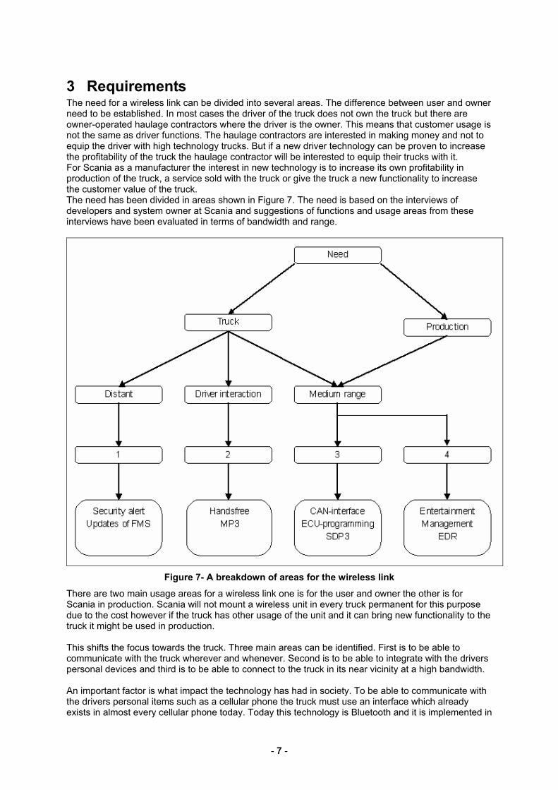
3 Requirements The need for a wireless link can be divided into several areas. The difference between user and owner need to be established. In most cases the driver of the truck does not own the truck but there are owner-operated haulage contractors where the driver is the owner. This means that customer usage is not the same as driver functions. The haulage contractors are interested in making money and not to equip the driver with high technology trucks. But if a new driver technology can be proven to increase the profitability of the truck the haulage contractor will be interested to equip their trucks with it. For Scania as a manufacturer the interest in new technology is to increase its own profitability in production of the truck, a service sold with the truck or give the truck a new functionality to increase the customer value of the truck. The need has been divided in areas shown in Figure 7. The need is based on the interviews of developers and system owner at Scania and suggestions of functions and usage areas from these interviews have been evaluated in terms of bandwidth and range.

Figure 7- A breakdown of areas for the wireless link

There are two main usage areas for a wireless link one is for the user and owner the other is for Scania in production. Scania will not mount a wireless unit in every truck permanent for this purpose due to the cost however if the truck has other usage of the unit and it can bring new functionality to the truck it might be used in production. This shifts the focus towards the truck. Three main areas can be identified. First is to be able to communicate with the truck wherever and whenever. Second is to be able to integrate with the drivers personal devices and third is to be able to connect to the truck in its near vicinity at a high bandwidth. An important factor is what impact the technology has had in society. To be able to communicate with the drivers personal items such as a cellular phone the truck must use an interface which already exists in almost every cellular phone today. Today this technology is Bluetooth and it is implemented in

- 8 - 8

a large number of cellular phones today and will probably continue to be implemented in these devices in the near future. Some cellular phone manufacturer has started to implement WLAN in their latest business phones [4]. Several PDA manufacturers are implementing WLAN in most of their new PDA’s however these PDA’s also have Bluetooth [5-6]. It is possible that all phones and PDA’s has a WLAN connection interface in the future however it will probably take some time before it has become common to have WLAN in the PDA or in the phone. In the mean time Bluetooth is the best alternative since it is widely adopted today. This is marked as 2 in Figure 7. For long distance communication with the truck today the GSM and GPRS system is used. The main reason for this is that the infrastructure of GSM network already exists and has good coverage in Europe. Even in some African countries the GSM network has good coverage. An alternative for this today is satellite communication but the cost for data traffic is much higher than GSM. It is possible that GSM is replaced by another technology when the infrastructure changes however these system changes slowly [7]. This is marked as 1 in Figure 7. This leave the intermediate communication open for further studies. As said prior in this thesis the customer and user are often not the same which means that an intermediate communication must be cost effective. Functions implemented with this technology must be directed towards the haulage contractor rather than the driver. This is marked as 3 and 4 in Figure 7. One function that is directed towards both the driver and the haulage contractors is traffic updates in the navigator. These updates could give the driver information about traffic jams and give him an alternative route which would make his route much more efficient and the utilization of the truck can be increased. System with similar functionality is the Scania interactor and toll collect system used in Germany. These systems both have a GSM and GPS. There is a possibility that other countries implements another system which would mean that a truck which travels from one country to another may have to use two different toll collect system since this is not standardized. These systems are similar to the interactor and could probably be replaced with the interactor. This would reduce the weight, cost, fuel consumption and power consumption of the truck. United States Department of Transportation envisions a vehicle to vehicle and vehicle to infrastructure communication in every new motor vehicle in the future [8].

- 9 - 9

4 New concept

4.1 Short term concept Based on the function areas previously discussed a short term implementation plan for some of these areas were made. By separating the GPRS modem and interactor and by adding a CAN to GPRS gateway additional functionality which uses long distance communication can be introduced. For example the trucks security system could then send data such as GPS position to a security company when the security system detects an intrusion. The interactor still needs to be able to use the GPRS modem without affecting the CAN bus. Another area is the driver interaction and because it is legislated to use hands free while driving in most of Europe it is likely that customers will request a fixed hands free system in the truck. The only wireless technology that can be used for this is Bluetooth since it is a highly adopted technology in cellular phones today. To affect the system at a minimum only the status of the buttons for controlling this system is sent on the CAN bus. Audio from such a system should be connected directly towards the speakers in the truck and a microphone has to be mounted in the truck as well. The third functions area covers medium range systems such as programming in production and diagnostics at a workshop. If a wireless unit is connected temporally to the diagnostic connector during the assembly of the truck. It could be used to program and test the ECU’s in the truck. A wireless link in production could decrease the assembly time if the programming and testing of ECU’s could be done while other parts are mounted on the truck. This would also simplify the production line because it could reduce some of the ECU programming stations. It is not unlikely that workshops will want to use a wireless link for diagnostics. Then the trucks DTC could be read while the truck is in the parking lot and a time slot in the workshop could be reserved rather than doing the diagnostics when the truck is inside the workshop. Software upgrades could be done while the truck is parked outside the workshop. It is likely that the workshops will want to use a Scania approved wireless link for this. Then Scania can recommend or even certify the product that they use in production. How this can be implemented in today’s system architecture can be viewed in Figure 8.

- 10 - 10

Figure 8- Overview of the short term implementation in today's system architecture

There is always a security risk when a wireless link is used. By only using temporary nodes for direct access to the CAN network with a WEP encryption where the key often is changed the security can be considered strong. However information such as immobilizer codes should never be sent over a wireless link. The gateway between CAN and GPRS should only be able to gate specific data which has been determined as “safe” meaning they can not affect the handling, behavior and security of the truck.

- 11 - 11

4.2 Long term concept By introducing a high speed bus for information the wireless CAN interface, interactor and other systems can send data without affecting the integrity of the CAN bus. The information on this high speed bus must not contain information between systems other than the wireless gateway and one node or the ICL and a node. This will ensure that system crucial data is transported on the CAN bus and not on the high speed bus. By doing so the robustness of the CAN is preserved which is important from a safety point of view. If data from a unit were sent on the CAN bus the busload and performance in transmission time would be affected. An example of this is an Electronic Driver Recorder (EDR). If the EDR collects vehicle speed every second and the data stored has the size of one byte. It will result in data about 86 kB every 24 hour. If the data is sent in CAN messages with 8 bytes of data in every message it would result in 10750 CAN messages. By sending a CAN message every 10 ms which corresponds to 6.5%1 of the maximum busload it would take about 18 minutes. 6.5% increase in busload is not acceptable because it would affect the CAN bus to much. It is more realistic to send a CAN message every 1 second which would correspond to 0.06% busload. Then the total transmission time would be 3 hours. This calculation is based on the fact that 8 byte in each CAN message is used for data in reality some of this data would have to be some sort of identifier for the data. How this calculation was made is shown in Equation 1.

ondsinfrequenssendingmessageCANeveryinsent

TotaltimeonTransmissi

ondsondeverycollectedTotal

tD

DT

tDD

sec______

_

secsec__

⋅

=

⋅=

−

Equation 1 - Calculation of sending time

This shows how little data can affect the busload on the CAN bus. But if a high speed bus were implemented the data could be transferred faster to the wireless gateway without affecting the CAN bus. A telecommunications system is today used for fleet management it is likely that it will be used in the future for communications when it is important to reach the truck within a short time period. An example of this is order handling or changes in the route of the truck. According to “Roadmap wireless systems 2005 to 2010” [7] the change of telecommunications systems comes slowly, it is an evolution rather than a revolution. GPRS will probably be used until another alternative with at least the same coverage, speed and cost is available. Data which is not critical when it arrives is used in other kind of management systems an example of this is EDR or vehicle management. In these systems the data is used for statistics and to determine service and economics of the truck. It can be collected automatically when the truck arrives to the haulage contractor. For this kind of transmission a medium range communication system is better. Today WLAN offers good performance for this communication. It is not unlikely that a wireless OBD communication will be standardized by SAE or ISO and if it is it would be appropriate to be able to use this medium for other types of medium range communication as well if it offers adequate performance. Today Bluetooth is the technology for communication with the driver’s cellular phone and it will probably be Bluetooth in the future too but not the same version as today. The development of Bluetooth is done continuously and will probably stay highly adopted because it is compatible with older Bluetooth devices. Since a high speed bus is implemented it can be used by other systems too. An example of this is the ICL which could be used as a display in a video phone call or show mini map from the navigator if it were connected to the high speed bus.

1 Measured value on an idle bus with CANalyzer 5.1

- 12 - 12

An example of which system that could participate in the high speed bus can be viewed in Figure 9. The gateway will have at least three types of wireless links long distant GPRS or 3G, medium range WLAN, C2C or DSRC and Bluetooth for driver interaction. The gateway should have two bus connections one to the CAN bus and one to the high speed bus. Then any ECU can request a service from the gateway and the wireless mediums can access the high speed bus for large data streams.

Figure 9- Example of the high speed bus implementation in today’s system architecture

Since there are two workgroups car to car communication consortium (C2C) and dedicated short range communication (DSRC) working on vehicle to vehicle communication it is not unlikely that some form of standard will be drafted. The main usage areas of these are traffic safety but they may also include entertainment functions and toll collect system. From a security point of view wireless communication media with high bandwidth should be considered a larger threat towards unauthorized communications than low bandwidth wireless communications due to this and the usage areas of the high speed bus some guidelines is proposed for the high speed bus.

• System critical data will be sent on CAN and not on the high speed bus. • The high speed bus should be considered unreliable in terms of robustness. • Never communicate security keys on this bus. • A malfunction on high speed bus will not affect the handling and performance of the truck. • Consider all traffic on this bus public broadcast to every one. • Software updates in ECU’s requires an authentication of a mechanic.

- 13 - 13

5 Technology

5.1 Technology presentation The most common standards for wireless communication will be considered in this thesis and they are Bluetooth, Zigbee, Wi-Fi / WLAN, GSM/GPRS and WiMAX. Open frequencies are used by Scania in the security system today. Open frequencies is not standardized but there are regulations of these frequencies. The signal power is regulated and the technology is common in security systems in the automotive industry. Open frequencies will not be considered any further in this thesis. A short description containing general information, performance, frequency, error correction, network structure and how mature the technology is will be presented in the following way. General description General description with history and usage areas. Network properties The network is described on terms of topology and nodes. Performance A description of the performance of the standard in terms of bit rate. Error handling A description of how error detection and error correction is made. Radio and security properties A description of modulation technique and security mode for the standard. Other aspects How mature the technology is and special aspects of this technology. The technology presentation will be concluded with an evaluation and comparison of the different technologies. Some technical terms are explained further in Appendix A.

5.1.1 Bluetooth

5.1.1.1 General description Bluetooth is an open specification for a short range wireless communication any where in the world. It is publicly available and royalty free. In 1994 Telefonaktiebolaget LM Ericsson started a project studying the feasibility of a low-power and low-cost radio interface to eliminate cables between mobile phones and their accessories [9]. To make the technology widely accepted and adapted on the market an industry group that could produce an open and common specification were formed. In May 1999 the Bluetooth special interest group (SIG) was publicly announced.

5.1.1.2 Network properties When two or more Bluetooth devices are in range they can automatically establish a connection as a piconet. One of the devices takes the role of master and the others become slave. The master doesn’t have any special privilege it only governs the synchronization and frequency hopping spread spectrum. A piconet can have one master and up to seven active slaves and 255 slaves in parked mode. In parked mode a slave maintains synchronization with the master but is no longer considered active. By using parked mode the master can direct the communications in a piconet with more than seven slaves. A device can participate in more than one piconet, it is then called a scatternet. The hopping sequence is different for each piconet. The rules of a piconet apply to the scatternet, so a device can be slave in both piconets, but it can also be slave in one piconet and master in another [9]. The range of Bluetooth is about 10 meters by class three devices which uses a signal power of 0 dBm (1 mW). Class one devices has a range of 100 meters and uses a signal power of 20 dBm (100 mW).

- 14 - 14

Figure 10- Bluetooth network topology

5.1.1.3 Performance Bluetooth has a capacity of 1 Mega symbol per second supporting the bit rate of 1 Megabit per second. 64 kbps per second is dedicated for voice [10]. The bit rate is 721 kbps for asymmetrical transfers but only allowing 57.6 kbps upstream and for symmetrical transfers the bit rate is 432 kbps.

5.1.1.4 Error handling To detect errors two methods are used. The header of the message is checked for errors using a header error check (HEC) generated by a generator polynomial. The header contains link control data and consists of 18 bits where 10 bits is data and 8 bits is used for error correction [11]. The data also called as payload is checked by using a cyclic redundancy check (CRC) of two bytes. The received data is also controlled with a 24 bit control word to distinguish which piconet it belongs to. There are three ways to make an error correction 1/3 FEC, 2/3 FEC and ARQ 1/3 FEC uses a simple repetition in sending of the header bits [11]. 2/3 FEC uses a shortened hamming code. Each block of 10 bit information is coded into a 15 bit control word. This code can correct all single errors and detect all double errors in each codeword. In the automatic repeat request scheme most data packets shall be transmitted until acknowledgement of successful repetition is returned by the destination (or time is exceeded).

5.1.1.5 Radio properties and security Bluetooth operates at a frequency between 2,400 and 2.4835 GHz which is divided in to 79 channels but in some countries only 23 channels is used. Every channel is 1 MHz wide. The data which are to be sent is divided into small packets which are sent in sequence over different frequencies. This is called frequency hopping or frequency hopping spread spectrum (FHSS) and by using this technique RF interference on one transmission can be reduced. If a collision with another transmission occurs or a packet is damaged on one channel the packet will just be retransmitted on new channel. If several Bluetooth devices are operating in the same area there is a chance of collision between the devices. By spreading the packets evenly over the frequency spectrum and only occupying the channel for a short period of time (nominally the frequency is changed every 625 ms [11]) the chance of collision is reduced [9]. Four different authentication entities are used by the link layer for maintaining security: Bluetooth device address, two secrete keys and a pseudorandom number. The Bluetooth device address is obtained by a user or automatically in an inquiry routine. The two secrete keys are derived during the initialization and are never disclosed. One is for authentication and the other is for encryption. When encryption is activated a new encryption key shall be generated. The encryption key can vary between 8 and 128 bit in byte wise length [11]. By using a shorter key less computer capacity have to be implemented in the Bluetooth device.

- 15 - 15

5.1.1.6 Other aspects Today Bluetooth is commonly used in cellular phones. There are many devices that use Bluetooth technology. Some of these devices are wireless headsets, synchronization between the device and computers schedules and address books. The cost of implementing Bluetooth is today considered low. Bluetooth can be used in almost every country in the world. The highest layer of the Bluetooth stack is the application layer which contains the different profiles of Bluetooth. There are several profiles on the market today and many new ones are under development. The most interesting for Scania today is the Headset profile. This profile makes it possible to make a wireless communication between an onboard hands free system in the truck and the driver’s personal phone. There is another profile which will become interesting for Scania when it is fully developed. This profile is under development by the car workgroup profile at Bluetooth SIG. They work on implementing the following usage models [10].

5.1.1.6.1 Usage Models: • Operating a phone via an in-car device • Portable device exports its user interface to the car • Personalizing the car and its devices • Remote car-access • Call handling between car-embedded and portable phones • Remote access to the car position • Car to environment communication • Diagnostics and programming • Operating a communication device in a hands-free mode specifically related to Automotive

- 16 - 16

5.1.2 Wireless local area network WLAN / Wi-Fi IEEE802.11

5.1.2.1 General description Wireless Local Area Network (WLAN) was developed by a workgroup of the Institute of Electrical and Electronic Engineers (IEEE). There are four standards available today 802.11, 802.11a, 802.11b and 802.11g. 802.11a operates at 5 GHz and the other operates at 2.4 GHz. When 802.11 were standardized it had a capacity of 2 Mbps but soon there were products on the market that offered proprietary solutions with a capacity of 11 Mbps. To stop a segmentation of the market a complementary standard was released 802.11b. This standard became available on the market before 802.11a standard which may seem strange. The work on 802.11a started before the 802.11b hence the order of the names. The main difference between 802.11 standards lies is the physical layer. The 802.11g standard is fully compatible to 802.11 and 802.11b standards. The 802.11a standard is not compatible with the other standards since it operates on a different frequency. The 802.11a standard uses the same MAC layers as all 802.11 physical layers so it can easily be implemented with another type of 802.11 modules.

5.1.2.2 Network properties All the standards have the same network structure. They can be configured for either an ad hoc network or use an Access point. In an ad hoc network nodes can communicate directly with other nodes which are in the physical range of the node however some nodes have to work as a router if the receiver is out of range from the transmitting node. If the network is constructed of access points they control the routing of messages between nodes. If the access points are connected to each other either by a physical conductor or a wireless link they can route transmissions between nodes connected to different access points.

Figure 11- WLAN network topology

The reach of a node using an 802.11 standard is not specified however the output power is specified and is an important factor when determine the reach of a node which is about 100 m to 300 m outdoor and 30 m to 100 m indoor2. It is not uncommon for transmission speed to decrease when distance between nodes increase.

5.1.2.3 Performance The different 802.11 standards offer bit rates between 2 Mbps and 54 Mbps. 802.11 offers a bit rate of 2 Mbps and 802.11b offers a bit rate of 11 Mbps. Both 802.11a and 802.11g offer a bit rate of 54 Mbps. An overview of the bit rates for the different standards is given in Table 2. 2 Estimated value

- 17 - 17

Standard Bit rate (Maximum)802.11 2 Mbps 802.11a 54 Mbps 802.11b 11 Mbps 802.11g 54 Mbps

Table 2- Overview of the 802.11 standards

5.1.2.4 Error handling In the MAC layer each frame includes a Frame Check Sequence (FCS), which contains a 32-bit CRC for error detection [12]. 802.11a uses FEC with coding rate of 1/2, 2/3 or 3/4 in the physical layer [13].

5.1.2.5 Radio properties and security 802.11 uses Frequency hopping spread spectrum (FHSS) for 1 Mbps and Direct sequence spread spectrum (DSSS) for 2 Mbps. At 2.4 GHz 802.11b operates like the DSSS version of 802.11on 14 different channels in the 2.4 GHz band (2412-2484).Because of different legislations in different countries all channels are not available in all countries this can be viewed in Table 3 [14]. The 802.11b standard uses Complementary Code Keying (CCK) for the new bit rates and the older 11-chip Barker sequence and DBPSK or DQPSK for the lower bit rates. 802.11g standard uses orthogonal frequency division multiplexing OFDM.

Channel Frequency [MHz] US/Canada Europe Japan 1 2412 X X X 2 2417 X X X 3 2422 X X X 4 2427 X X X 5 2432 X X X 6 2437 X X X 7 2442 X X X 8 2447 X X X 9 2452 X X X 10 2457 X X X 11 2462 X X X 12 2467 N/A X X 13 2472 N/A X X 14 2484 N/A N/A X

Table 3- Overview of channels and frequencies

802.11a operates in the 5 GHz frequency and uses orthogonal frequency division multiplexing encoding scheme rather than FHSS or DSSS [15]. There is a disadvantage with using the 5 GHz band. The shading at 5 GHz is more severe compared to 2.4 GHz and depending on the SNR, propagation conditions and the distance between sender and receiver, data rates may drop fast. In the 802.11 standard a wired equivalent privacy (WEP) algorithm is specified. When it was specified it was considered to be reasonably strong [12] but today it should be considered weak because there are programs (wepcracker and airsniffer are examples of this) available which can decipher the encryption key within a few hours by just listening to the data traffic. There are other ways to protect a wireless network but they are not specified in the 802.11 standard.

5.1.2.6 Other aspects To asses how well adopted the different standards are one can look at how new laptops and handhelds are equipped. Almost all new laptops have WLAN implemented with the exception of the low price laptops. The majority of laptops have 802.11b or 802.11g standard there are also some laptops with all the three standards. Another indicator is the price of a WLAN module in large volumes. With this as a basis it can be assumed that 802.11b and 802.11g is the most common standards.

- 18 - 18

5.1.3 Zigbee

5.1.3.1 General description By using Bluetooth or WLAN a high bit rate can be achieved, these technologies is suitable for high speed communication such as streaming audio, video, PC-LAN and synchronization of phonebooks. There is an area which is not covered by Bluetooth and WLAN. This area is measurements in large scale network with low power and cheep modules. This is what started the Zigbee Alliance. The name Zigbee comes from the bumblebee’s way of communication where the bumblebee dances in a zigzag pattern. Zigbee is a relative new technology it was standardized in December of 2004 and today there are some components available on the market.

5.1.3.2 Network properties There are only two physical devices available, this is for keeping a low system cost for Zigbee products. Full Function Device (FFD) and Reduced Function Device (RFD). FFD Can function in any network topology Capable of being the network coordinator Capable of being a network router Can talk to any other device

RFD Limited to star network topology Cannot become a network coordinator Can only talk to a network coordinator Very simple implementation

An IEEE 802.15.4/ Zigbee network requires at least one FFD as a network coordinator but the end point devices can be RFD. There are two main network topologies star network and peer-to-peer however these two can be combined into a third one which is called meshed network. The different network topologies can be viewed in Figure 12, Figure 13 and Figure 14.

5.1.3.2.1 Star network A FFD can be configured to create its own network and become a Personal Area Network (PAN) coordinator. The other FFD and RFD can then connect to the PAN. All network nodes which are in range of the radio sphere must have a unique PAN identity to be able to connect to the network. All communication between nodes must go through the network coordinator.

Figure 12- Star network topology

5.1.3.2.2 Peer-to-Peer network When the Peer-to-Peer topology is used a PAN network coordinator must exist however the communication between nodes do not have to go through the network coordinator. The nodes can communicate directly with each other.

- 19 - 19

Figure 13- Peer-to-peer network topology

5.1.3.2.3 Meshed network When a meshed network is used there is only one network coordinator but all FFD nodes works as a router to direct communication between nodes in the shortest and most reliable way. The network is also able to heal it self by rerouting the communication if a node is disabled.

Figure 14- Meshed network topology

5.1.3.3 Performance The bit rate of Zigbee is dependent of the frequency used. At 868.0-868.6 MHz the maximum bit rate is 20 kbps, 902-928 MHz the maximum bit rate is 40 kbps and at 2.4 GHz the maximum bit rate is 250 kbps.

5.1.3.4 Error handling Error detection is done by a Frame Check Sequence (FCS) mechanism employing a 16-bit International Telecommunication Union –Telecommunication standardization Sector (ITU-T) Cyclic Redundancy Check (CRC) and is used to protect every frame.

5.1.3.5 Radio properties and security Zigbee is based on the IEEE 802.15.4 standard which operates at three different frequencies with 27 channels, 16 channels at 2.4000 to 2.4835 GHz, ten channels at 902 to 928 MHz and one channel at 868.0 to 868.6 MHz. The lower frequencies 868.0-868.6 MHz and 902- 928 MHz use a binary phase shift keying (BPSK) modulation. The 2.4 GHz frequency band uses a more sophisticated modulation technique. The bit stream is mapped into symbols of 4 bits. The symbol is then transformed into a chip value of 32 pseudorandom bits which is sent by applying an O-QPSK modulation. There are three types of security modes unsecured mode, access control list, secure mode.

5.1.3.5.1 Unsecured mode No security is used.

5.1.3.5.2 Access control list Only communications from known devices is accepted and the communication is not encrypted.

- 20 - 20

5.1.3.5.3 Secure mode There are four different security services which can be used Access control list, Data encryption Frame integrity check and Sequential freshness

5.1.3.5.4 Data encryption Data encryption uses an Advanced Encryption Standard (AES) it uses a 128-bit encryption.

5.1.3.5.5 Frame Integrity Frame integrity uses a Message Integrity Code (MIC) to protect data from being modified by a node without the correct encryption key.

5.1.3.5.6 Sequential freshness Sequential freshness uses an ordered sequence of inputs to reject communications which have been replayed, by comparing the freshness value of a received message with the freshness value of the previously message the rejections and acceptance of messages is determined.

5.1.3.6 Other aspects Zigbee is designed to be a low price module, the cost is about 3 $ when ordering about 1000 units with PHY/MAC layer and Zigbee stack [16]. Low power consumption can be achieved by letting the node sleep for a larger part of their lifetime. To be able to do this a short wakeup time is required. Zigbee has a short wakeup time it takes typically 15 ms for a node to go from sleeping mode to active mode. The connection time for a new node is also small it is typically 30 ms [17]. The 2.4 GHz band operates worldwide while frequencies below 1 GHz operates in North America, Europe and Australia/New Zealand. The Zigbee stack is considered to be 1/4th of the Bluetooth and IEEE 802.11 stack.

- 21 - 21

5.1.4 Worldwide Interoperability for Microwave Access WiMAX

5.1.4.1 General description WiMAX was developed for metropolitan area network usage with high bit rate and long range. WiMAX is designed for point to multipoint broadband wireless access. WiMAX will provide fixed, portable and eventually mobile wireless broadband. WiMAX is based on IEEE 802.16 and two types of communications are defined. They are communication with nodes in the Line Of Sight (LOS) and nodes Not in the Line Of Sight (NLOS).

5.1.4.2 Network properties The range of WiMAX is going to be typically 3 to 10 kilometers. WiMAX uses a meshed network structure. Base stations can communicate with each other and some or all of them are connected to an Internet service provider (ISP) through a physical connection. Subscriber stations can then connect to a base station and access the internet. An example of the network structure can be viewed in Figure 15.

Figure 15- An example of a WiMAX network

5.1.4.3 Performance WiMAX uses a variable bandwidth between 1 MHz and 28 MHz this allows raw bit rates of 120 Mbps. WiMAX system can be expected to deliver 40 Mbps per channel for fixed and portable devices. Mobile network deployments can be expected to provide 15 Mbps.

5.1.4.4 Error handling CRC-32 is used for error detection of PDUs for all automatic repeat connections. FEC is also used in the PHY layer there are four different types of FEC.

5.1.4.4.1 Code Type1: Reed-Solomon This case is useful either for large data block or when high coding rate is required

5.1.4.4.2 Code Type2: Reed-Solomon + Block conventional code This case is useful for low to moderate coding rates providing good carrier to noise ratio (C/N) enhancements.

5.1.4.4.3 Code Type3: Reed-Solomon + Priority check This optional code is useful for moderate to high coding rates with small to medium size blocks. The parity code can be used for error correction.

5.1.4.4.4 Code Type4: Block Turbo Code (BTC)

- 22 - 22

This optional code is used to significantly lower the required carrier to interference ratio (C/I) level needed for reliable communication and can be used to either extend the range of a base station or the code rate for greater throughput.

5.1.4.5 Radio and security properties NLOS operates in a frequency band between 2-11 GHz and LOS in the frequency band of 11-66 GHz. Another standard is being drafted 802.16e which shall give WiMAX mobility. NLOS was specified in IEEE802.16a standard which is implemented in the IEEE802.16 standard available today. The IEEE802.16 standard covers both MAC layer and PHY layer. In the PHY layer both frequency division duplex and time division duplex can be used. Active modulation allows WiMAX system to adjust the signal modulation scheme depending on the SNR condition of radio link. When the signal has high quality the highest modulation scheme is used. This gives the system more capacity. An overview of when modulation scheme is changed for different SNR is concluded in Table 4.

SNR (dB) Modulation scheme 6 BPSK 9 QPSK 16 16 QAM 22 64 QAM

Table 4- An overview of modulation scheme depending of SNR

The connection between a base station and subscriber station is encrypted and this provides a good protection against theft of the service. If a subscriber station specifies that it does not support IEEE802.16 security. Step of authorization and key exchange shall be skipped. If subscriber station can not be authenticated it shall not be serviced [18]. There are two component protocols for privacy. An encapsulation protocol for encrypting packet data across the fixed broadband wireless access (BWA) network. This protocol defines a set of supported cryptographic suites and rules for applying those algorithms to a MAC PDU payload [18]. A key management protocol (PKM) providing the secure distribution of keying data. Data encryption can either be done with US Data Encryption Standard (DES) using algorithm (FIPS 46-3, FIPS 74, FIPS 81) or data encryption can be done with US Advanced Encryption Standard (AES) algorithm (NIST special publication 800-38C, FIPS 197) to encrypt the MAC PDU payload [19].

5.1.4.6 Other aspects Since WiMAX is a new technology it is considered a rather expensive technology. Today one WiMAX receiver for an end user costs about 5000 SEK. The goal for Intel is that in a few years a WiMAX receiver should cost the same as a WLAN card costs today. It has been tested for one year in Skellefteå, Sweden, with good results [20].

- 23 - 23

5.1.5 Telecommunication GSM/GPRS/3G

5.1.5.1 General description GSM is the most successful digital mobile telecommunication system in the World today. It is used by 800 million people in over 190 countries. GSM is the second generation (2G) telecommunications system. GSM sends data and voice in the same way to improve the capacity for sending data GPRS was developed as an extension of GSM. When GPRS is used the user is generally charged by transferred data and not by the connection time. The third generation of mobile communications system (3G) is also known as Universal Mobile Telecommunications System (UMTS). In late 1998 the European Union (EU) decided that all EU countries should make it possible for an introduction of 3G system at the latest at January first 2002. The biggest difference between UMTS and GSM is the radio interface. Speech may be the most widely used service. Speech has certain requirements in terms of data rate, delay and error free delivery. All which are derived from human perspectives and expectations. Speech quality in UMTS has to be at least as good as in the 2G wireless network [21]. UMTS uses several coding algorithms and code rates, one is used in the 2G network GSM enhanced full rate coding scheme. The reuse of coding algorithms and coding schemes means that voice-coding should at least have the same quality as the 2G network. UMTS specification defines four service classes where the services within a given class have a common set of characteristics

5.1.5.1.1 Conversational This is characterized by low delay tolerance, low delay variation and low error tolerance. The data flow is generally symmetrical [21].

5.1.5.1.2 Interactive This consists of typically request/response type transaction. It is characterized by low tolerance for errors but larger tolerance for delays than conversational services. The data rate demand depends on the services [21].

5.1.5.1.3 Streaming This concerns one-way services, using low to high bit rates. Streaming services have a low error tolerance but generally have a high tolerance for delay. This is because receiving application usually buffers the data so it can be synchronized when it is replayed to the user [21].

5.1.5.1.4 Background This is characterized by little if any delay constraint. Examples include server to server e-mail delivery, SMS, and performance/measurement reporting. Background application requires error free delivery [21].

- 24 - 24

5.1.5.2 Network properties Telecommunications networks consist of several base transceiver stations (BTS). BTS can form a radio cell alone or together with other BTS [15]. A radio cell has a range between 100m and 35km depending on its surroundings. The BTS is connected to a Base station controller which is a part of the network and switching subsystem and together with the operating system they form a mobile telecommunications network. An example of this can be viewed in Figure 16.

Figure 16- An example of a mobile network

5.1.5.3 Performance GSM provides a bit rate of 9.6 kbps while moving in speeds up to 250 km/h. GPRS offers a more powerful bit rate than GSM by using the available network in a more effective way. The maximum bit rate is 171.2 kbps but typical receiving bit rate is 53.6 kbps and a sending bit rate of 26.8 kbps [15]. The bit rate is depending of which code scheme and how many time slots are being used. The achieved bit rates can be viewed in Table 5 according to used code scheme and timeslots. GPRS can use up to 8 slots.

Slots Coding scheme 1 2 3 4 5 6 7 8 CS-1 (kbps) 9.05 18.20 27.15 36.20 45.25 54.30 63.35 72.40 CS-2 (kbps) 13.40 26.80 40.20 53.60 67.00 80.40 93.80 107.20CS-3 (kbps) 15.60 31.20 46.80 62.40 78.00 93.60 109.20 124.80CS-4 (kbps) 21.403 42.80 64.20 85.603 107.00 128.40 149.80 171.20

Table 5- GPRS data rates for coding schemes and time slots

UMTS offers a bit rate of 144 kbps for vehicular traffic, 348 kbps for pedestrians and 1910 kbps for fixed objects [21].

3 Properties of the GPRS modem used by Scania.

- 25 - 25

5.1.5.4 Radio properties and security GSM has initially been deployed in Europe using 890-915 MHz for uplinks and 935-960 MHz for downlinks, this system is referred to as GSM900. There are two newer versions GSM1800 and GSM1900. GSM1800 uses 1710-1785 MHz for uplink and 1805-1880 MHz for downlink. GSM1900 uses 1850-1910 MHz for uplink and 1930-1990 MHz for downlink [15]. GPRS uses a Time Division Multiple Access (TDMA) which allows several devices to share the same frequencies by dividing the time in to timeslots. Allocation of the slots is based on current load and operator preferences. Operators often reserve at least one timeslot per TDMA frame to guarantee a minimum data rate. All GPRS services can be used in parallel to conventional services [15]. GPRS offers four different coding schemes (CS) which offer different speeds of the transmission they also have less reliability and error correction. The choice of coding scheme depends on the condition of the channel provided by the cellular network (quality of the radio link between GPRS node and base station). If the channel is very noisy, the network may use lowest coding scheme to ensure higher reliability if the channel is providing a good condition the network could use a higher coding scheme to obtain optimum speed. GPRS devices are divided into different classes in order of how many timeslots they can occupy. Table 6 shows an example of GPRS device classes.

Class Maximum number of receiving slots

Maximum number of sending slots

Maximum number of slots

1 1 1 2 2 2 1 3 3 2 2 3 5 2 2 4 8 43 13 53 10 44 2 5 12 4 4 5

Table 6- Example of GPRS device classes

The biggest difference between UMTS and GSM is the new radio interface WCDMA. It uses a Direct Sequence Code Division Multiple Access (DS-CDMA). In Europe 1900-1920 MHz is used for TDD modulation, 1920-1980 MHz and 2110-2170 MHz is used for FDD modulation with a 190 MHz carrier spacing.

5.1.5.5 Other aspects Scania uses GPRS for communication between the truck’s and the central fleet management system. To establish the connection a Siemens MC35i GPRS modem is used. It is a class 8 modem. It has a maximum download bit rate of 85.6 kbps and a maximum sending bit rate of 21.4 kbps. Siemens MC35i modem operates with GSM900 and GSM1800 systems.

3 Properties of the GPRS modem used by Scania.

- 26 - 26

5.2 Technology in development Research in vehicle to vehicle communication is conducted in both Europe and America. The intent for this is to increase the safety on the roads. If vehicles are given the ability to communicate with each other they can send warning messages about fog, ice and obstacles in the road such as road works or traffic jams. The vehicle which receives a message can then inform the driver and if necessary recalculate the route. There are enormous possibilities for traffic safety measures if the communication and technology is standardized. The functions of such a standard will not be considered any further in this thesis. However two research project and technical approaches will be explained.

5.2.1 Dedicated Short Range Communication Dedicated Short Range Communication is developed in America by an interest work group which started its work in 1999 [22]. Their goal is to create a general standard for vehicle to road side and vehicle to vehicle communication for short and medium range. This DSRC should not be confused with the existing DSRC at 915 MHz. The new DSRC is base on IEEE802.11 standards and will operate on a 5.9 GHz frequency, have a range up to 1000 m and a bit rate of 6 to 27 Mbps on seven licensed channels. Due to the fact that a 5.9 GHz module is not developed yet DSRC will use the available IEEE802.11a standard. It is very similar so the implementation of the 5.9 GHz module should only require small changes. It will also have directed antennas which can be directed towards a specific lane however this is a disadvantage when reaching a wide area. DSRC is intended to use standardized chip and software to reduce the cost of the technology. The work group for DSRC has many visions for the usage of the technology and has worked with the project for about six years but today there is no DSRC system in production. The Federal communications commission has dedicated a 75 MHz band at 5.85 GHz to 5.925 GHz for DSRC in February 2004 [8]. In 2005 Daimler Chrysler Corporation which participates in the DSRC project used DSRC at 5.9 GHz to make a connection between two trucks that where following each other on the road and let the first truck control the second truck [23].

5.2.2 Car 2 Car Communication Consortium Car 2 Car Communication Consortium (C2C) is a European work group which works toward a European standard in vehicle to vehicle communication system. C2C also promote an allocation of a royalty free European wide exclusive frequency band. The C2C system is derived from the IEEE802.11 standard. When two or more vehicles are in radio contact they automatically establish an ad hoc network where every vehicle also functions as a router. The router algorithm is based on the position of the vehicles and is able to handle a fast changing ad hoc network structure. A basic concept is scheduled for release in 2005 and in the beginning of 2006 research guidelines are planned for release. In 2007 a draft of the full specification is scheduled and in 2008 the specification will hopefully be input to standardization. During 2010 a frequency allocation is scheduled [24].

- 27 - 27

5.3 Evaluation of technology The different technologies were developed for different purposes therefore they have different characteristics in terms of bandwidth and network topology. The areas covered by these technologies are summarized in Figure 17.

Figure 17- Areas covered by different technologies

A more technical overview of the technologies is made in Table 7.

Zigbee Bluetooth WLAN WiMAX GPRS 3G Network size 65 000 7 (255)* 32 100>x<1000 Global Countries Bandwidth (kbps) 20-250 720 54 000 40 000 171 1920 Range (m) ~100 ~10 ~100 ~30 000 - - Cost / unit quantity

3$ 1000

<5$ 1000

<3$ 10 000

600$ 1

- -

Characteristics Cost Power

Cost Adaptation

Speed Flexibility

Range Speed

Coverage Flat rate

Coverage Speed

Table 7- A technical data overview

Since an interface towards the CAN bus is the most interesting for Scania in both a technical and a production point of view the characteristics for this type of communication is considered. This interface needs to be able to handle a two way communications bus at 250 kbps if different types of tests are going to be conducted. The tests towards a truck considered in this thesis is programming ECU’s in production, Communication between vehicles and using Scania’s diagnostics program through a wireless link. By looking at the fact that a speed of 250 kbps in two directions is required the Zigbee and GPRS technology can be discarded. A 3G solution is not appropriate either because it is a telecommunications system which is intended for long distance communication and another aspect is the bit rate which drops to about 144 kbps when moving in vehicular speeds. WiMAX is a very new technology which means it is rather expensive and it has not been deployed in a large scale yet. It has the bandwidth capacity but it has not been specified for mobile purposes yet. This leaves Bluetooth and WLAN. Bluetooth has a rather short range if not a class one module is used but Bluetooth also has a tendency to drop in bit rate with the increase of distance between the modules due to the SNR ratio of Bluetooth. This leaves WLAN which has a high bit rate and good

- 28 - 28

range which makes it the best candidate for these tests. Another advantage of WLAN is that DSRC and C2C is being based on this technology. A disadvantage is that it is not intended for mobile usage at the speeds of heavy vehicles which is about 90 km/h. The weak encryption in the WEP algorithm is not crucial for these tests since the range is limited and most of the test is conducted on Scania’s test area. All this together indicates that a WLAN solution is preferred.

5.4 Testing of the technology

5.4.1 Test equipment There were not many products available on the market. One was Sorcus CANbox which had been used in the SAINT project by KTH. The CANbox solution was initially borrowed from KTH for a short evaluation. In the evaluation a transfer test revealed that some messages disappeared but the supplier had a new firmware which would fix this problem so two CANbox units were purchased. Each CANbox can handle two independent CAN buses. The CANbox offers speeds up to 1 Mbps on the CAN bus and are compliant to CAN specification 2.0A and 2.0B. It uses the IEEE802.11b standard for the wireless link which can establish either an ad hoc network or use a router for the network. Up to 10 CANbox units can be used simultaneously on a single PC or PDA. The CANbox is powered with 6 to 60 volts. Two different antennas came with the CANbox units when they were purchased one small and one large. The small antenna had a gain of 2.1 dBi and the large antenna had a gain of 5.1 dBi [25]. The antennas can be viewed in Figure 18.

Figure 18- Photo of the antennas. The small antenna at the top

Two main programs have been used during the tests, CANalyzer and matlab. CANalyzer is a development tool which has been used to write programs for sending and receiving data over the CAN bus. The data on the CAN bus have been logged in ASCII files. The CANalyzer program is written in a C-like program language which is called CAPL. The ASCII files has then been converted to matlab data files and analyzed in matlab programs. The Source code for the CANalyzer programs can be viewed in Appendix B and the matlab programs can be viewed in Appendix C.

- 29 - 29

5.4.2 In lab environment

5.4.2.1 Transfer test To determine the maximum transfer capacity of the CANbox a CANalyzer program was written. The program can control the frames sent per second by adjusting two parameters the burst of messages and the time between the bursts. By starting at a frame rate of 1500 frames per second (fps) it could be determined that the maximum rate for a CANbox is 1400 fps because the maximum output at 1500 fps were 1400 fps. Several different fps were tried with different antennas. By measuring lost frames, delay time and busload a reliable speed for transferring data in lab environment can be determined. The transfer test was done three times for every speed. The result was analyzed with a matlab. In each test 150,000 CAN messages were sent. By maintaining the sending rate during 150,000 messages the durability of the frame rate is tested.

5.4.2.2 Delay test To determine how the busload and the number of lost messages affects the delay time, a program was written in CANalyzer which sends a message and waits until it has received the CAN message before sending the next CAN message. The delays occur when sending the CAN messages through the CANbox units rather then using a cable. The log files in this test were analyzed with matlab program. The results from this test were then compared to the transfer test.

5.4.2.3 Startup test The startup time is the time it takes for the CANbox unit to start sending or receiving data from the time when power is switched on. This was measured by sending data from one CANbox to the other with a CANalyzer program and then disconnecting power for a short time. The disconnected time was measured with an oscilloscope. Another purpose of this test was to determine if the configuration of client/server on the CANbox affected the startup time.

5.4.2.4 Programming and flashing test By replacing the cable between the vehicle communications interface (VCI) and the OBD interface with two CANbox units the ECU’s can be programmed in the same way as when a cable is used. At the start of the test no filtration on the CAN messages were done but after the first test a filter for KW2000 messages were configured on the unit connected to the OBD interface. The filter only allows the CANbox to relay KW2000 messages all other CAN messages will be ignored. This reduces the amount of traffic on the wireless link. How the connection was made can be viewed in Figure 19. All programming were made in a lab environment and on lab equipment at Scania’s department for diagnose development RESD.

Figure 19- Connection between VCI - CANbox and CANbox - OBD

- 30 - 30

5.4.3 In the Truck

5.4.3.1 Placement of the CANbox antenna To determine how the placement of the CANbox affects the range a simulation was made at Swedish national Testing and Research institute (SP). Simulations were made with a FDTD program which used a simplified CAD-model of a Scania truck cabin including seats and steering wheel/column modeled as metal. The CAD-model can be viewed in Figure 20. The truck cabin had no rear window and on this truck the fuel tanks were mounted behind the cabin. The CAD model lacked some interior attributes such as dashboard and some exterior such as driving mirrors.

Figure 20- Simplified CAD-model

Two different positions were simulated for the CANbox antenna. In addition to the simulations measurements were made in the EMC protected room at SP. Since the CANbox units only send small packages of data it is difficult to measure the amplitude of the electric filed. By making a simplified antenna from a small metal box and the small antenna from the CANbox and connecting it to a signal generator the electric field could be measured in some directions. A figure of the simplified antenna can be viewed in Figure 21.

- 31 - 31

Figure 21- Simplified antenna

The electric field was measured with a horn antenna on parts of a circle (81-99, 171-189, 261-279 and 357-3 degrees) with a radius of 5 meters where the centre was at the CANbox antenna position. The position of the simplified antenna can be viewed in Figure 22 and Figure 23.

Figure 22- The simplified antenna placed on the dashboard in the truck

- 32 - 32

Figure 23- The simplified antenna placed among most of the other electrical control units

5.4.3.2 Tracking test To determine a frame rate when two trucks is following each other the large antenna were placed on the roof of the trucks. The lead truck was loaded with a container. The lead truck can be viewed in Figure 24. Both trucks were equipped with a CANbox and a laptop computer running CANalyzer. The first truck then sent data at a specific frame rate to the truck driving behind the first truck. The second truck held normal distance to the truck in the front. The driving speeds varied between 30 km/h to 90 km/h. The log files were analyzed in matlab in terms of number of lost frames, average delay, maximum delay, minimum delay, average busload and maximum busload on both receiving and sending bus. The tests were performed two times for each fps tested (1100, 800, 700, 600, 500 fps).

Figure 24- The lead truck loaded with a container

- 33 - 33

5.4.3.3 SDP3 To be able to use SDP3 over a wireless link the CANbox units were connected between the VCI and OBD contact which can be viewed in Figure 19. The CANbox connected to the OBD contact was configured as client with a pass filter for KW2000 CAN messages and also without a pass filter.

5.4.4 In production

5.4.4.1 EOL programming By replacing the cable between the VCI and the OBD contact at the EOL programming station with two CANbox units the EOL programming could be done wireless. The CANbox connected to the OBD contact was configured as client with a pass filter for KW2000 CAN messages. The connection can be viewed in Figure 19.

- 34 - 34

5.4.5 Test result

5.4.5.1 Transfer test The result from the transfer test is summarized in two tables (Table 8 and Table 9) one for each antenna type. The result is also visualized in graphs for the different measured attributes which is found in Appendix D. Fps 1100 1200 1250 1300 1333 1375 1400Average number of errors 0.00 0.00 0.67 30.67 7.67 0.00 1326.33 Average delay time (s) 0.14 0.15 0.13 0.16 0.12 0.14 0.32 Max delay time (s) 0.29 0.23 0.30 0.35 0.31 0.24 2.06 Min delay time (s) 0.00 0.01 0.01 0.02 0.02 0.02 0.02 Average sending busload (%) 65.13 71.09 73.99 77.03 78.97 81.44 83.10 Average receiving busload (%) 64.36 70.15 73.08 76.05 78.03 80.47 81.20 Difference in busload (%) 0.77 0.94 0.91 0.98 0.94 0.97 1.90 Max sending busload (%) 66.59 72.41 75.19 78.61 80.20 82.90 84.90 Max receiving busload (%) 66.23 71.69 76.31 80.63 80.93 81.50 81.50

Table 8- Overview of the results from the transfer test with the large antenna

Fps 1100 1200 1250 1300 1333 1375 1400Average number of errors 0.00 0.00 0.00 0.00 31.33 72.67 563.67 Average delay time (s) 0.17 0.17 0.17 0.17 0.18 0.19 0.30 Max delay time (s) 0.21 0.20 0.22 0.25 0.33 0.35 0.57 Min delay time (s) 0.00 0.00 0.00 0.00 0.00 0.00 0.00 Average sending busload (%) 65.15 71.07 74.03 77.12 79.00 81.48 83.09 Average receiving busload (%) 64.34 70.16 73.07 76.04 77.86 80.47 81.73 Difference in busload (%) 0.81 0.91 0.96 1.08 1.14 1.01 1.36 Max sending busload (%) 67.61 72.90 75.19 78.59 80.56 82.90 84.69 Max receiving busload (%) 66.58 71.90 75.55 80.50 81.69 82.51 82.98

Table 9- Overview of the results from the transfer test with the small antenna

As the tables shows the highest frame rate which is successful on all CAN messages with both antennas are 1200 fps which is about 71% busload. When all CAN messages are successfully transmitted the maximum delay is 290 ms and the average delay for all successful transmissions is 160 ms.

- 35 - 35

Overview

0.00

0.05

0.10

0.15

0.20

0.25

0.30

0.35

1100 1200 1250 1300 1333 1375 1400Fps

Tim

e (s

)

0

200

400

600

800

1000

1200

1400

Err

ors

Average delay, large antenna Average delay, small antennaErrors , large antenna Errors, small antenna

Figure 25- Overview of errors and delay time

The smaller antenna has a smother result compared to the results from the large antenna which is rather fluctuated for the different frame rates. When frames are lost it increases the delay time for other messages. When frames are lost they are often located next to each other and it happens when the frame rate is high.

5.4.5.2 Delay test The result from the delay test which where performed three times can be viewed in Table 10.

Test number Errors Maximum delay (s) Minimum delay (s) Average delay (s) 1 0 0.0254 0 0.0029 2 0 0.0253 0 0.0029 3 0 0.0252 0 0.0029

Table 10- Overview of the results from the delay test

No frames where lost while performing this test and the low minimum delay probably derives from the fact that the CANalyzer real-time clock has a lower resolution than the shortest delay. The maximum and average delay is much smaller in this test compared to the transfer test. The main reason for this difference is the fact that the bus was idle when the CAN message was sent and only one message is sent at the time.

5.4.5.3 Startup test The result from the startup test is summarized in Table 11. When the CANbox was configured as a server it did not fully recover from the restart. The transmission rate became limited which increased the transmission time.

Configuration Average startup time (s) Sending node / Client 11.9 Receiving node / Client 12.6 Sending node / Server 10.05 Receiving node / Server 15.25

Table 11- Overview of the results from the startup test

This test shows that the start up time for a client node is about 12-13 seconds. It also indicates that a server node is not capable to fully repair the connection when a power failure occurs. If one unit are to be connected and disconnected which is the case with a diagnostic tool, it should be configured as a client.

5 The transmission did not fully recover after the restart

- 36 - 36

5.4.5.4 Programming and flashing test The programming of ECU’s worked on OPC unit but the coordinator could not be programmed because a time out error occurred. The response time from the coordinator was to long and therefore a filtration was configured on the CANbox unit. When this was done all programming of the ECU’s worked and the programming times can be viewed in Table 12.

Type Connection Filter Total time (s) OPC Cable - 89 OPC CANbox No 196 Difference 107

OPC Cable - 89 OPC CANbox Yes 156 Difference 67

EOL Cable - 104 EOL CANbox Yes 105 Difference 1

Coordinator Cable - 48 Coordinator CANbox Yes 58 Difference 10

Table 12- Programming times for some ECU's

Since normal busload is about 30% the traffic through the CANbox can be reduced by ignoring all messages but the KW2000 messages which is used for diagnostics and programming. By doing this the programming time for the OPC ECU was reduced by 40 seconds. In general the programming worked but the programming time was substantial increased which indicates that it is not possible to implement it directly in production today. The EOL programming was only affected by 1 second. This type of programming could be implemented without changing anything in the production of dashboards.

- 37 - 37

5.4.5.5 Placement test The measured azimuth pattern for some directions can be viewed in Figure 26. For the directions where the driving mirrors blocked the line of sight between the CANbox antenna and the horn antenna the driving mirrors were turned forward. This was done because the driving mirrors were not modeled in the simulations. The fuel tanks had an impact on the electric field in the rear direction since they were mounted behind the cabin of this truck. Table 13 explains the relation between the angel in the azimuth figures and the direction of the truck.

Figure 26- Measured azimuth pattern

Phi (degrees) Direction on the truck0 Backwards 90 Right side 180 Front 270 Left side

Table 13- Relation between angel (Phi) and the truck

A simulated azimuth pattern for the two different placements of the CANbox antenna can be viewed in Figure 27. The placement on the dashboard had a stronger signal power in general than the placement by the other electrical units. Figure 28 and Figure 29 visualizes the simulated azimuth pattern with the measured pattern for both placements.

- 38 - 38

Figure 27- Simulated azimuth with no rear window

Figure 28- Simulated and measured azimuth pattern for the antenna at the dashboard

- 39 - 39

Figure 29- Simulated and the measured azimuth pattern for the antenna at the electric units

Additional simulation was done with a CAD-model which had a rear window these simulations can be viewed in Figure 30.

Figure 30- Simulated azimuth pattern for a truck with a rear window

- 40 - 40

The simulation shows that the placement among the other electrical units in general had a lower signal power than the placement on the dashboard. The simulations were confirmed by measurements done in some directions. The signal power was rather low behind the truck. Even a truck with a rear window had a generally low signal power in the rear direction. If communications between trucks are to be done an external antenna has to be used. This also shows the main disadvantage of placing the CANbox antenna inside the truck.

5.4.5.6 Tracking test The result from the transfer test when two trucks are following each other is summarized in Table 14. The result is also visualized in graphs for the measured attributes which is found in Appendix E.

Fps 500 600 700 800 1100 Average number of errors 0 0 16004 2055.5 52015

Average delay time (s) 0.72 0.42 1.62 1.28 2.06 Maximum delay time (s) 3.90 1.64 6.16 5.28 4.39 Minimum delay time (s) 0.00 0.01 0.00 0.01 0.02

Average sending busload (%) 26.58 35.41 40.65 45.00 62.55 Average receiving busload (%) 28.45 34.90 36.35 41.94 41.21 Difference in busload (%) 3.00 0.51 5.00 6.69 21.34

Maximum sending busload (%) 30.39 36.20 42.50 48.90 66.80 Maximum receiving busload (%) 50.70 57.86 62.63 78.80 54.63

Table 14- Overview of the results from the tracking test

The variations in lost frames and delay time over different frame rates indicate that the CANbox units lose the connection between each other. This can be viewed in Figure 31.

Overview

0

0.5

1

1.5

2

2.5

500 600 700 800 1100

Fps

Tim

e (s

)

0

10000

20000

30000

40000

50000

60000

Average delay Average error

Figure 31- Overview of errors and delay time

The highest frame rate for when all CAN messages are transmitted successfully is 600 fps which correspond to a busload of about 35%. The CANbox units place all messages in a buffer before they are sent and if there is no connection the buffer can be filled therefore a function for removing old or messages which is out of date will be necessary. The test mainly shows that the technology works at vehicular speeds with reduced frame rate compared to the lab results.

- 41 - 41

5.4.5.7 SDP3 When no filter was used the SDP3 program could not connect to the truck because of a time out error. By applying a filtration in the same way as in the programming and flashing test the SDP3 program worked. However if SDP3 was to be used two times in a row the CANbox units needed to be restarted because they locked up.

5.4.5.8 ECU-programming When ECU programming was tested on the development line in production only EOL worked. The other types of programming failed as a result of a timeout error. When EOL programming was tested in real production it worked on 4 to 5 dashboards then the connection seemed to fail and the operator had to retry for 5 to 10 times before it started to work. When another 4-5 dashboards have been programmed the reconnection is impossible and both CANbox units need to be restarted.

- 42 - 42

5.5 Result summary The study of function areas could conclude that there are four main areas where a wireless node is needed. These are: short distance at medium bandwidth, long distance at low bandwidth, medium distance at a high bandwidth towards the fleet management system and at medium distance at a high bandwidth towards the CAN bus and the ECU units. The medium range with a high bandwidth towards the CAN bus were the most interesting for Scania. The study in standardized wireless technologies concluded that the WLAN technology is most appropriate for communications towards the CAN bus. There are also needs for a bluetooth connection and a telecommunication connection but these are not the most interesting for Scania. The transfer test could conclude a maximum error free rate of 1200 fps in a lab environment. 1200 fps corresponds to about a 71% busload on the CAN bus. The average delay for 1200 fps was 170ms and the maximum was 200ms. The tracking test could conclude a maximum error free transfer rate of 600 fps between two moving trucks. 600 fps corresponds to about a 35% busload on the CAN bus. The average delay for 600 fps was 420ms and the maximum was 1.64s during this test. The delay test could conclude a maximum delay of 25ms. The startup test could conclude a start uptime about 12-13s and that the CANbox configured as server can not be restarted during a transmission. Flashing and programming test could conclude that programming and flashing is possible in lab environment. The programming time was increased when an ECU was flash programmed. For the OPC ECU it took 196s using a wireless node without a filter and 156s using a wireless node with a filter. Using a cable took 89s. For the COO ECU it took 58s to do a flash programming with a wireless node which used a filter and 48s using a cable. The EOL programming took 104s using a wireless node with a filter and 105s when a cable was used. EOL programming at the dashboard line in Oskarshamn worked but only for a few dashboards in a row. Then the CANbox needed to be reseted. SDP3 could be used but only if both CANbox units were restarted before a connection to the truck was made with SDP3. A placement of the antenna inside the truck reduced the electric field behind the truck enough to make a communication between two trucks almost impossible with the standardized signal powers.

- 43 - 43

5.6 Applications and their benefits and limitations

5.6.1 On a Truck The main benefit of implementing some sort of wireless communication on a truck is the new functionality which can be a benefit in customer value. If information from the CAN network can be shared between trucks a lot of new functionality can be implemented however there is no standardized protocol for how this communication should work. This is the main limitation for inter vehicle communication another large limitation is to keep the integrity of the CAN network when an external node want to share information with the trucks internal system. If a new function is going to be profitable for Scania the customer has to be willing to pay extra for it unless it can offer some thing that Scania’s competitors can not offer and the customer request it.

5.6.2 Workshops and SDP3 If a truck can be diagnosed or just have a software upgrade without having to bring the truck in to the workshop the workshop can be utilized in a more effective way. One large disadvantage is the security of the wireless link, the immobilizer code needs to be protected or even better never be communicated over the wireless link. If a permanent node is used for this the authentication of a workshop need to be solved in a way so that only authorized personal can update the software in the truck.

5.6.3 In Production By replacing the VCI cable with a wireless connection the assembly line could be reconfigured. The ECU units could be programmed continuously during the assembly as soon as the dashboard is powered up. This would reduce the number of programming stations. It would also reduce the production stops which occur when the cable from the VCI to the OBD contact gets stretched and breaks. The main limitation is that the timeout limits and packet burst in the programming software has to be reconfigured to work better with the CANbox. The programming time will be longer with the CANbox. Since immobilizer codes are sent over a wireless link an encryption of the traffic is necessary the CANbox offers a 128-bits WEP encryption which today is approved by Scania but in the future it will probably be considered weak because there are programs which can decode the encryption key by listening to the data traffic for a few hours.

- 44 - 44

6 Conclusion Of the technologies studied the WLAN technology is best suited for communications towards the CAN network. The technology has been tested and works, however all of the properties of the CAN bus can not be sustained in the wireless link and due to this all communications should be handled trough a gateway. Bluetooth was not appropriate for communications towards CAN because the SNR ratio causes the bandwidth to drop rather fast with the distance. A permanent wireless gateway should also come with the implementation of a high speed bus for increased functionality and maintaining the integrity of the CAN bus. The EOL programming through the CANbox units works. The CANbox units had some problems but the WLAN technology has been proved to work. The problem with the CANbox units can probably be fixed by doing some further studies. CANbox is not appropriate to use for communications between vehicles due to the limited filtering functions and the lack of access control and the lack of freshness control of the CAN messages in queue for sending. However the WLAN technology works for this kind of communication. The placement of the antenna for a wireless communications gateway is crucial. Placing the antenna inside the cabin will result in substantial reduction of the signal power in the backwards direction. The CANbox is not appropriate to use with the SDP3 because the CANbox units locked up when the VCI was restarted but it can be profitable for the workshops to use a wireless CAN link of some sort to be able to update trucks without having to bring them inside the workshop.

- 45 - 45

7 Recommendation for further research

• To investigate if a WLAN router can fix the problems with the CANbox units locking up. By using a WLAN router the CANbox units do not need to handle the change in network structure.

• To investigate if the communication between the CANbox and the VCI is causing the CANbox

units to lock up.

• Closely monitor the development in the American DSRC project and the European C2C project.

• Closely monitor the development of the Bluetooth car work group which is specified by

Bluetooth SIG.

• Measure and simulate the placement of a roof mounted antenna.

• Investigate if it is possible to connect power to the dashboard while building it and there by enabling the possibility to program the dashboard continually during the assembly.

• To investigate the performance of the CANbox if CAN messages are sent directly from a PC’s

WLAN card to the CANbox.

• To test other types of WLAN to CAN links to see if they work better than the CANbox units.

- 46 - 46

8 References [1] Scania, www.scania.com, 2005-09 [2] Robert Bosh, Bosch CAN specification version 2.0, 1991 [3] ISO14229-1, Road Vehicles – Unified diagnostic services (UDS – part 1: specification

and requirements), ISO, 2004-01-13 [4] Nokia, http://www.nokia.com, 2005-10 [5] Palm, http://www.palm.com, 2005-10 [6] Compaq, http://www.compaq.com, 2005-10 [7] Bo Karlsson, Östen Mäkitalo, MatsNilson and Jens Zander, Roadmap Wireless

Systems 2005 to 2010, Wireless@KTH 2005 06 10, seminar at Wireless@KTH Kista on September 16 2005

[8] Federal communication commission, FCC 03-324, 2004-02-10 [9] Brent A. Miller and Chatschik Bisdikian, Bluetooth Revealed –The insiders guide to an

open specification for global wireless communications, Prentice Hall 2001, ISBN: 0-13-090294-2

[10] The Bluetooth Special Interest Group, http://www.bluetooth.org 2005-10 [11] Specification of the Bluetooth System – core Version 1.1 February 22 2001 [12] Wireless LAN IEEE standards 802.11, IEEE 1999, ISBN: 0-731-1658-0 [13] Wireless LAN IEEE standards 802.11a, IEEE 1999, ISBN: 0-7381-1810-9 ss94787 [14] Wireless LAN IEEE standards 802.11b, IEEE 1999, ISBN: 0-7381-1812-5 ss94788 [15] Jochen Schiller, Mobile Communication (second edition), Pearson Education Limited

2003, ISBN: 0-321-12381-6 [16] Freescale semiconductor, http://www.freescale.com, 2005-10 [17] Zigbee Alliance, http://www.zigbee.org, 2005-10 [18] Zigbee IEEE standards 802.15.4, IEEE 2003, ISBN: 0-7381-3677-5 ss95127 [19] Wireless MAN IEEE standards 802.16, IEEE 2004, ISBN: 0-7381-4070-8 ss95246 [20] Nyteknik, http://www.nyteknik.se/pub/ipsart.asp?art_id=41297, 2005-10 [21] Clint Smith and Collins Daniel, 3G Wireless networks, New York McGraw-Hill cop.

2002, ISBN: 0-07-1414827-5 [22] Armstrong consulting, http://www.leearmstrong.com, 2005-09 [23] DaimlerChrysler, http://www.daimlerchrysler.com, 2005-10 [24] Car2Car Communication Consortium, http://www.car-to-car.org, 2005-09 [25] Sourcus computer GmbH, CANbox dual CAN to WLAN/LAN converter,

www.sorcus.com, 2005-07-12

- 47 - 47

9 Appendix A A short explanation of different terms such as modulation techniques.

9.1 FHSS Frequency Hopping Spread Spectrum Frequency hopping spread spectrum is a technique that enables multiple networks in the same area. The frequency band is divided in 79 channels for USA and Europe and 23 channels for Japan. Every channel has a bandwidth of 1 MHz. Different networks are separated by different hopping sequences. The selection of channel is determined by a pseudorandom hopping pattern.

9.2 DSSS Direct Sequence Spread Spectrum DSSS is an alternative way to separate the spectrum by using code and not by using frequency. Spreading is achieved by using the 11-chip Barker sequence. The signal is spread across a wider frequency band which is in direct proportion to the number of bits used. Therefore 11-chip separation uses an 11 times wider frequency band than a single bit would require. The key characteristics of this method are its robustness against interference and its insensitivity to multipart propagation.

9.3 CCK Complementary Code Keying Complementary code keying contains a pair of finite bit sequences of equal length, such that the number of pairs of identical elements (1 or 0) with any given separation in one sequence is equal to the number of pairs of unlike elements having the same separation in the other sequence. A network using CCK can transfer more data per unit time for a given signal bandwidth than a network using the Barker code, because CCK makes more efficient use of the bit sequences.

9.4 DQPSK Differential Quadrature Phase Shifting Keying DQPSK does not use a relative phase shift to a reference signal [15]. It uses the phase of the previous two bits to determine the phase shift. The receiver does not need the reference signal but only compare two signals to reconstruct data.

9.5 DBPSK Differential Binary Phase Shift Keying When BPSK is used the phase may become shifted by some effect in the communications channel which the signal passes through. This problem can be overcome by using the data to change rather than set the phase. In BPSK a binary ’1’ may be transmitted by adding 180° to the current phase and a binary ‘0’ by adding 0° to the current phase.

9.6 OFDM Orthogonal Frequency Division Multiplexing By using OFDM the signal is divided in smaller parts which are sent simultaneously on narrowband channels at different frequencies. OFDM reduce the amount of crosstalk in signal transmissions.

9.7 TDMA Time Division Multiple Access Time Division Multiple Access allows several devices to share the same frequencies by dividing the time in to timeslots [15]. The TDMA frame time slots are not allocated in a fixed predetermined manner but on demand. All time slots can be shared by the active users, up and down link are allocated separately.

9.8 DS-CDMA Direct Sequence Code Division Multiple Access DS-CDMA multiplies a stream of pseudo random bits with a chipping sequence this spread the signal and if the chipping sequence is unique it can separate different users. All signals use the same frequency band. To separate different users the code for spreading should be (quasi) orthogonal, in other words their cross relation should be almost zero

- 48 - 48

9.9 O-QPSK Offset Quadrature Phase Shift Keying O-QPSK modulates the even bits on to a Carrier phase (I) and odd bits on the quadrature phase carrier (Q). To form the offset between the I-phase and Q-phase the Q-phase is delayed by Tc were Fc is the center frequency.

9.10 Pseudorandom A pseudorandom process is a process that appears random but is not. Pseudorandom sequences typically exhibit statistical randomness while being generated by an entirely deterministic computational process

9.11 QAM Quadrature Amplitude Modulation QAM is a modulation scheme which conveys data by changing the amplitude of two carrier waves. These two waves, usually sinusoids, are out of phase with each other by 90 degrees and are thus called quadrature carriers. The number in front of QAM specifies which order the modulation is. With a higher order it is possible to transmit more bits per symbol.

9.12 Barker sequence A Barker code is a string of digits ai= ±1 of length l ≥ 2 such that

∑−

=+ ≤

kl

ikii aa

1

1

For all 1 ≤ k < l. Barker sequences are used for pulse compression of signals. There are barker sequences of lengths 2, 3, 4, 5, 7, 11, and 13, and it is conjectured that no longer Barker codes exists.

9.13 Reed-Solomon Reed-Solomon error correction is a coding scheme which works by first constructing a polynomial from the data symbols to be transmitted and then sending an over sampled plot of the polynomial instead of the original symbols themselves. Because of the redundant information contained in the over sampled data, it is possible to reconstruct the original polynomial and thus the data symbols even in the face of transmission errors, up to a certain degree of error.

9.14 CRC Cyclic Redundancy Check Given a k-bit block of bits, or message, the transmitter generates a frame check sequence ((n-k)-bit sequence) such that the resulting frame (consisting of n-bits) is exactly divisible by some pre determined number. The receiver can then divide the incoming frame with that number and if there is no reminder the frame is considered to have no errors.

- 49 - 49

10 Appendix B Source code for CANalyzer programs.

10.1 Transfer_sender.CAN The sourcecode for the CANalyser program used in the transfer test, tracking test, and passing test. /*@@var:*/ variables { const WORD SEND_BUS = 3; // Selects CAN channel const WORD RECE_BUS = 4; // Selects CAN channel message 0x100 sendingMSG; mstimer sendingTimer; mstimer stopTimer; mstimer synchTimer; DWORD StartID = 0x0x; DWORD Time_now; BYTE sendingBurst=0; BYTE timeBetweenBurst =0; BYTE idCounter = 0; WORD Messagelimit= 0; WORD stopTime = 10000; // delay after last message is received WORD dataCounter = 0; INT i,j; } /*@@end*/ /*@@startStart:Start:*/ on start { //Test cases // Fps ID TIME Count // 500 5 10 30000 // 600 6 10 25000 // 700 7 10 21428 // 800 8 10 18750 // 1100 11 10 13636 // 1200 12 10 12500 // 1250 10 8 15000 // 1300 13 10 11539 // 1333 12 9 12500 // 1375 11 8 13636 // 1400 14 10 10714 writeclear(1); setParam (5, 10, 30000); //Sets the parameters for the test case write("Press 's' to synchronize test"); write("Press 't' to start test"); } /*@@end*/ /*@@key:'s':*/ on key 's' { Write("Starting"); // sends first synchronization message sendingMSG.CAN = SEND_BUS; sendingMSG.ID = 0xF0000x; sendingMSG.DLC = 8; Time_now = timeNow(); sendingMSG.long(0) = Time_now; sendingMSG.long(4) = 0x00000000; output(sendingMSG); settimer(synchTimer, 1000); // start timer for sending the next synchronization message } /*@@end*/

- 50 - 50

/*@@caplFunc:sendMsg():*///function sendMsg () // Function for sending a message and increasing the data in the message { sendingMSG.CAN = SEND_BUS; while(idCounter < sendingBurst) { sendingMSG.ID = StartID+(idCounter * 0x10000); sendingMSG.DLC = 8; sendingMSG.long(0) = 0x00000000 + dataCounter; sendingMSG.long(4) = 0x00000000; output(sendingMSG); idCounter++; } idCounter=0; dataCounter++; } /*@@end*/ /*@@timer:sendingTimer:*/ on timer sendingTimer { canceltimer(sendingTimer); sendMsg(); if(dataCounter < Messagelimit) settimer(sendingTimer, timeBetweenBurst); else { settimer(stopTimer, 5000); } } /*@@end*/ /*@@timer:stopTimer:*/ on timer stopTimer { Write("Messure Finnished"); stop(); } /*@@end*/ /*@@caplFunc:setParam(word,word,word):*///function setParam (Word burst, Word timeb, Word MSGlim) { sendingBurst = burst; timeBetweenBurst = timeb; Messagelimit = MSGlim; Write("New properties is Sending Burst = %d, Time = %d, MSG = %d ",sendingBurst,timeBetweenBurst,MSGlim ); } /*@@end*/ /*@@timer:synchTimer:*/ on timer synchTimer // sends second synchronization message { sendingMSG.CAN = SEND_BUS; sendingMSG.ID = 0xF0000x; sendingMSG.DLC = 8; Tidnu = timeNow(); sendingMSG.long(0) = Tidnu; sendingMSG.long(4) = 0x00000000; output(sendingMSG); //Stars tot send all messages } /*@@end*/ /*@@key:'t':*/ on key 't' { settimer(sendingTimer, timeBetweenBurst); } /*@@end*/

- 51 - 51

10.2 Delay test The sourcecode for the CANalyser program used in the delay test. /*@@var:*/ variables { const WORD SEND_BUS = 3; // Selects CAN channel const WORD RECE_BUS = 4; // Selects CAN channel message 0x100 sendingMSG; mstimer sendingTimer; mstimer stopTimer; WORD dataCounter = 0; WORD stopTime = 10000; // Time to wait until messurment stops after the last message in ms DWORD StartID = 0x0x; DWORD recievedMSG[15][15000]; DWORD sentMSG[15][15000]; INT i,j; INT times = 1; LONG Message_count; } /*@@end*/ /*@@startStart:Start:*/ on start { writeclear(1); write("Press 's' to start test"); Message_count = 50000; } /*@@end*/ /*@@key:'s':*/ on key 's' { Write("Starting"); sendMsg(); } /*@@end*/ /*@@caplFunc:sendMsg():*///function sendMsg () // Function for sending messages and increasing the data in the message { sendingMSG.CAN = SEND_BUS; if(dataCounter < Message_count) { sendingMSG.ID = StartID; sendingMSG.DLC = 8; sendingMSG.long(0) = 0x00000000 + dataCounter; sendingMSG.long(4) = 0x00000000; output(sendingMSG); } else { write("dataCounter == %d", dataCounter); if(times < 3) { times++; dataCounter = 0; sendingMSG.ID = StartID; sendingMSG.DLC = 8; sendingMSG.long(0) = 0x00000000 + dataCounter; sendingMSG.long(4) = 0x00000000; output(sendingMSG); } else settimer(stopTimer, 10000); } dataCounter++; } /*@@end*/

- 52 - 52

/*@@timer:sendingTimer:*/ on timer sendingTimer { sendMsg(); } /*@@end*/ /*@@timer:stopTimer:*/ on timer stopTimer { Write("Messure Finnished"); stop(); } /*@@end*/ /*@@msg:*:*/ on PG * // When a message is received next message is sent { if(this.CAN == RECE_BUS) { sendMsg(); } } /*@@end*/

- 53 - 53

11 Appendix C Source code for the matlab programs.

11.1 Transfer test Since this test was performed on one computer no synchronization were made. The analyzing program consists of three matlab files start_analysing.m, analyse.m and analyseBusload.m.

11.1.1 start_analysing.m clear all; clc; Number_of_ID = 14; Send = load('small antenna\1400fps\sender_3.mat'); Receiver = load('small antenna\1400fps\mottagare_3.mat'); test=1; max_delay = zeros(1,Number_of_ID); min_delay = zeros(1,Number_of_ID); mean_delay = zeros(1,Number_of_ID); errors = zeros(1,Number_of_ID); Total_errors = 0; % Analyses the message matrixes and returns max, min mean delay and number of errors [max_delay(1), min_delay(1), mean_delay(1), errors(1)] = analyze(Send.Delay__ID_0__DATA_FROM_ID_0, Receiver.Delay__ID_0__DATA_FROM_ID_0); % Analyses the message matrixes and returns max, min mean delay and number of errors [max_delay(2), min_delay(2), mean_delay(2), errors(2)] = analyze(Send.Delay__ID_1__DATA_FROM_ID_1, Receiver.Delay__ID_1__DATA_FROM_ID_1); % Analyses the message matrixes and returns max, min mean delay and number of errors [max_delay(3), min_delay(3), mean_delay(3), errors(3)] = analyze(Send.Delay__ID_2__DATA_FROM_ID_2, Receiver.Delay__ID_2__DATA_FROM_ID_2); % Analyses the message matrixes and returns max, min mean delay and number of errors [max_delay(4), min_delay(4), mean_delay(4), errors(4)] = analyze(Send.Delay__ID_3__DATA_FROM_ID_3, Receiver.Delay__ID_3__DATA_FROM_ID_3); % Analyses the message matrixes and returns max, min mean delay and number of errors [max_delay(5), min_delay(5), mean_delay(5), errors(5)] = analyze(Send.Delay__ID_4__DATA_FROM_ID_4, Receiver.Delay__ID_4__DATA_FROM_ID_4); % Analyses the message matrixes and returns max, min mean delay and number of errors [max_delay(6), min_delay(6), mean_delay(6), errors(6)] = analyze(Send.Delay__ID_5__DATA_FROM_ID_5, Receiver.Delay__ID_5__DATA_FROM_ID_5); % Analyses the message matrixes and returns max, min mean delay and number of errors [max_delay(7), min_delay(7), mean_delay(7), errors(7)] = analyze(Send.Delay__ID_6__DATA_FROM_ID_6, Receiver.Delay__ID_6__DATA_FROM_ID_6); % Analyses the message matrixes and returns max, min mean delay and number of errors [max_delay(8), min_delay(8), mean_delay(8), errors(8)] = analyze(Send.Delay__ID_7__DATA_FROM_ID_7, Receiver.Delay__ID_7__DATA_FROM_ID_7); % Analyses the message matrixes and returns max, min mean delay and number of errors [max_delay(9), min_delay(9), mean_delay(9), errors(9)] = analyze(Send.Delay__ID_8__DATA_FROM_ID_8, Receiver.Delay__ID_8__DATA_FROM_ID_8); % Analyses the message matrixes and returns max, min mean delay and number of errors [max_delay(10), min_delay(10), mean_delay(10), errors(10)] = analyze(Send.Delay__ID_9__DATA_FROM_ID_9, Receiver.Delay__ID_9__DATA_FROM_ID_9); % Analyses the message matrixes and returns max, min mean delay and number of errors if(Number_of_ID > 10)

[max_delay(11), min_delay(11), mean_delay(11),errors(11)] = analyze(Send.Delay__ID_10__DATA_FROM_ID_10, Receiver.Delay__ID_10__DATA_FROM_ID_10);

end; % Analyses the message matrixes and returns max, min mean delay and number of errors if(Number_of_ID > 11)

[max_delay(12), min_delay(12), mean_delay(12),errors(12)] = analyze(Send.Delay__ID_11__DATA_FROM_ID_11, Receiver.Delay__ID_11__DATA_FROM_ID_11);

end % Analyses the message matrixes and returns max, min mean delay and number of errors; if(Number_of_ID > 12)

[max_delay(13), min_delay(13), mean_delay(13),errors(13)] = analyze(Send.Delay__ID_12__DATA_FROM_ID_12, Receiver.Delay__ID_12__DATA_FROM_ID_12);

end; % Analyses the message matrixes and returns max, min mean delay and number of errors if(Number_of_ID > 13)

[max_delay(14), min_delay(14), mean_delay(14),errors(14)] = analyze(Send.Delay__ID_13__DATA_FROM_ID_13, Receiver.Delay__ID_13__DATA_FROM_ID_13);

end; max = max(max_delay);

- 54 - 54

min = min(min_delay); Average = mean(mean_delay); Total_errors=sum(errors); start_Time = Receiver.Delay__ID_0__DATA_FROM_ID_0(1,1) +2; stop_Time = Send.Delay__ID_0__DATA_FROM_ID_0( size(Send.Delay__ID_0__DATA_FROM_ID_0,1)-1,1) -1; % calculates the bus load characteristics [Average_Busload_sending, Average_Busload_receiving, Max_busload_sending, Max_busload_receiving, Difference] = analyzeBusload(start_Time, stop_Time, Send.CAN3__BusLoad, Receiver.CAN4__BusLoad); Delay_text_1 = sprintf( 'Average delay = %.3f', Average); Delay_text_2 = sprintf( 'Max delay = %.3f', max); Delay_text_3 = sprintf( 'Min delay = %.3f', min); Busload_text_1 = sprintf( 'Average sending busload = %.3f',Average_Busload_sending); Busload_text_2 = sprintf( 'Average receiving busload = %.3f',Average_Busload_receiving); Busload_text_3 = sprintf( 'Difference in busload = %0.3f',Difference); Max_busload_text_1 = sprintf( 'Max sending = %0.3f',Max_busload_sending); Max_busload_text_2 = sprintf( 'Max receiving = %0.3f',Max_busload_receiving); ID_text = sprintf( 'Number of ID used = %d',Number_of_ID); Error_text = sprintf( 'Total number of errors = %d',Total_errors); disp('RESULT'); disp(' '); disp(ID_text) disp(Error_text); disp(' '); disp(Delay_text_1); disp(Delay_text_2); disp(Delay_text_3); disp(' '); disp(Busload_text_1); disp(Busload_text_2); disp(Busload_text_3); disp(' '); disp(Max_busload_text_1); disp(Max_busload_text_2);

11.1.2 analyseBusload.m function [average_send, average_rece, max_send, max_rece, diff_average] = analyzeBusload(startTime,stopTime,Send, Receiv) Send_elements = 0; Receive_elements = 0; i=1; Send_load = 0; Receiv_load = 0; Busload = 0; while(i < size(Send,1)) % summarize all busload elements between starttime and stoptime and counts the elements

Send(i); if(Send(i) > startTime && Send(i) < stopTime)

Send_elements = Send_elements +1; Send_load = Send_load + Send(i,2);

end; if(Receiv(i) > startTime && Receiv(i) < stopTime)

Receive_elements = Receive_elements +1; Receiv_load = Receiv_load + Receiv(i,2);

end; i = i+1;

end; Send_load = (Send_load / Send_elements) * 0.01; %calculates average busload and normalize it Receiv_load = (Receiv_load / Receive_elements) * 0.01; %calculates average busload and normalize it average_send =Send_load; average_rece = Receiv_load; max_send = max(Send(:,2))*0.01; max_rece =max(Receiv(:,2))*0.01; diff_average = abs(average_send - average_rece);

- 55 - 55

11.1.3 analyse.m function [maximum,minimum,average, errors] = analyze(Send,Receiv) Delay_Time(1:size(Receiv,1)-1)=0; i=1; j=1 % compares sent message matrix with received message matrix and stores the time difference in a vector ; while(i < size(Receiv,1))

if(Send(j,2) == Receiv(i,2)) % if the datat in the message is equal in sent and received the time is stored Delay_Time(i) = Receiv(i,1) - Send(j,1); i = i + 1; j = j + 1;

else % if the data is not equal a frame has been lost and next value from the sent matrix is tested j = j + 1;

end; end; errors = (j-i); maximum = max(Delay_Time); minimum = min(Delay_Time); average = mean(Delay_Time);

11.2 Delay test This analyzing program consists of two matlab files start.m and analyze.m.

11.2.1 start.m clear all; clc; Send = load('CANbox_lab\send1.mat.'); Receiver = load('CANbox_lab\mottagare1.mat'); Send.Delay__ID_0__DATA_FROM_ID_0; size(Send.Delay__ID_0__DATA_FROM_ID_0,1); size(Receiver.Delay__ID_0__DATA_FROM_ID_0,1); Delay_Time(1:size(Receiver.Delay__ID_0__DATA_FROM_ID_0,1))=0; % calculates time difference and stores result in an array i=1; j=1 %The sent message matrix is compared to the received and if the data in the message is the same the delay is stored in a vector and if it is not the same a frame has been lost and the next sent data is tested. while(i < size(Receiver.Delay__ID_0__DATA_FROM_ID_0,1))

if(Send.Delay__ID_0__DATA_FROM_ID_0(j,2) == Receiver.Delay__ID_0__DATA_FROM_ID_0(i,2)) Delay_Time(i) = Receiver.Delay__ID_0__DATA_FROM_ID_0(i,1) - Send.Delay__ID_0__DATA_FROM_ID_0(j,1);

i = i + 1; j = j + 1;

else j = j + 1;

end; end; %Results errors = (j-i) maximum = max(Delay_Time) minimum = min(Delay_Time) average = mean(Delay_Time) plot(Delay_Time);

11.3 Startup test This analyzing program only consists of the matlab file analyze_startuptime.m.

11.3.1 analyze_startuptime.m clear all; clc; load('test3/mätning2.mat'); ID0 = Delay__ID_10__DATA_FROM_ID_10; stoptid=0; starttid =0;

- 56 - 56

i=2; % By comparing the time for the received messages with the next message a time difference larger than 2 seconds will reveal the start and stop time of the time period when the CANbox were disconnected. while(i < size(ID0,1)) if((ID0(i,1)-ID0(i-1,1) > 2.0)) stoptid=ID0(i-1,1); starttid=ID0(i,1); end; i= i+1; end; %Results stoptid starttid totaltid =ID0(size(ID0,1),1) - ID0(1,1) -(starttid-stoptid) stem(ID0(:,1),ID0(:,2));

- 57 - 57

11.4 Tracking test The analyzing program for the tracking test is based on the program from the transfer test some alterations were made because of the need of synchronization between two computers and the number of unique CAN messages. The analyzing program consists of four matlab files start_analysing.m, analyze.m, Delay_time.m and analyzeBusload.m.

11.4.1 start_analysing.m clear all; clc; Number_of_ID = 5; Send = load('0500fps/send5.mat'); Receiver = load('0500fps/mottagare5.mat'); test=1; max_delay = zeros(1,Number_of_ID); min_delay = zeros(1,Number_of_ID); mean_delay = zeros(1,Number_of_ID); errors = zeros(1,Number_of_ID); Total_errors = 0; Delta_time = Delay_time(Send.Delay__Sync_mess__TIME(1,1), Receiver.Delay__Sync_mess__TIME(1,1),Send.Delay__Sync_mess__TIME(2,1), Receiver.Delay__Sync_mess__TIME(2,1)); if(Number_of_ID > 0)

[max_delay(1), min_delay(1), mean_delay(1), errors(1)] = analyze(Send.Delay__ID_0__DATA_FROM_ID_0, Receiver.Delay__ID_0__DATA_FROM_ID_0,Delta_time );

end; if(Number_of_ID > 1)

[max_delay(2), min_delay(2), mean_delay(2), errors(2)] = analyze(Send.Delay__ID_1__DATA_FROM_ID_1, Receiver.Delay__ID_1__DATA_FROM_ID_1,Delta_time );

end; if(Number_of_ID > 2)

[max_delay(3), min_delay(3), mean_delay(3), errors(3)] = analyze(Send.Delay__ID_2__DATA_FROM_ID_2, Receiver.Delay__ID_2__DATA_FROM_ID_2,Delta_time );

end; if(Number_of_ID > 3)

[max_delay(4), min_delay(4), mean_delay(4), errors(4)] = analyze(Send.Delay__ID_3__DATA_FROM_ID_3, Receiver.Delay__ID_3__DATA_FROM_ID_3,Delta_time );

end; if(Number_of_ID > 4)

[max_delay(5), min_delay(5), mean_delay(5), errors(5)] = analyze(Send.Delay__ID_4__DATA_FROM_ID_4, Receiver.Delay__ID_4__DATA_FROM_ID_4,Delta_time );

end; if(Number_of_ID > 5)

[max_delay(6), min_delay(6), mean_delay(6), errors(6)] = analyze(Send.Delay__ID_5__DATA_FROM_ID_5, Receiver.Delay__ID_5__DATA_FROM_ID_5,Delta_time );

end; if(Number_of_ID > 6)

[max_delay(7), min_delay(7), mean_delay(7), errors(7)] = analyze(Send.Delay__ID_6__DATA_FROM_ID_6, Receiver.Delay__ID_6__DATA_FROM_ID_6,Delta_time );

end; if(Number_of_ID > 7)

[max_delay(8), min_delay(8), mean_delay(8), errors(8)] = analyze(Send.Delay__ID_7__DATA_FROM_ID_7, Receiver.Delay__ID_7__DATA_FROM_ID_7,Delta_time );

end; if(Number_of_ID > 8)

[max_delay(9), min_delay(9), mean_delay(9), errors(9)] = analyze(Send.Delay__ID_8__DATA_FROM_ID_8, Receiver.Delay__ID_8__DATA_FROM_ID_8,Delta_time );

end; if(Number_of_ID > 9)

[max_delay(10), min_delay(10), mean_delay(10), errors(10)] = analyze(Send.Delay__ID_9__DATA_FROM_ID_9, Receiver.Delay__ID_9__DATA_FROM_ID_9,Delta_time );

end; if(Number_of_ID > 10)

[max_delay(11), min_delay(11), mean_delay(11),errors(11)] = analyze(Send.Delay__ID_10__DATA_FROM_ID_10, Receiver.Delay__ID_10__DATA_FROM_ID_10,Delta_time );

end; if(Number_of_ID > 11)

- 58 - 58

[max_delay(12), min_delay(12), mean_delay(12),errors(12)] = analyze(Send.Delay__ID_11__DATA_FROM_ID_11, Receiver.Delay__ID_11__DATA_FROM_ID_11,Delta_time );

end; if(Number_of_ID > 12)

[max_delay(13), min_delay(13), mean_delay(13),errors(13)] = analyze(Send.Delay__ID_12__DATA_FROM_ID_12, Receiver.Delay__ID_12__DATA_FROM_ID_12,Delta_time );

end; if(Number_of_ID > 13)

[max_delay(14), min_delay(14), mean_delay(14),errors(14)] = analyze(Send.Delay__ID_13__DATA_FROM_ID_13, Receiver.Delay__ID_13__DATA_FROM_ID_13,Delta_time );

end; max = max(max_delay); min = min(min_delay); Average = mean(mean_delay); Total_errors=sum(errors); start_Time = Receiver.Delay__ID_0__DATA_FROM_ID_0(1,1) +2; stop_Time = Send.Delay__ID_0__DATA_FROM_ID_0( size(Send.Delay__ID_0__DATA_FROM_ID_0,1)-1,1) -1; [Average_Busload_sending, Average_Busload_receiving, Max_busload_sending, Max_busload_receiving, Difference] = analyzeBusload(start_Time, stop_Time, Send.CAN3__BusLoad, Receiver.CAN4__BusLoad); Delay_text_1 = sprintf( 'Average delay = %.3f', Average); Delay_text_2 = sprintf( 'Max delay = %.3f', max); Delay_text_3 = sprintf( 'Min delay = %.3f', min); Busload_text_1 = sprintf( 'Average sending busload = %.3f',Average_Busload_sending); Busload_text_2 = sprintf( 'Average receiving busload = %.3f',Average_Busload_receiving); Busload_text_3 = sprintf( 'Difference in busload = %0.3f',Difference); Max_busload_text_1 = sprintf( 'Max sending = %0.3f',Max_busload_sending); Max_busload_text_2 = sprintf( 'Max receiving = %0.3f',Max_busload_receiving); ID_text = sprintf( 'Number of ID used = %d',Number_of_ID); Error_text = sprintf( 'Total number of errors = %d',Total_errors); disp('RESULT'); disp(' '); disp(ID_text) disp(Error_text); disp(' '); disp(Delay_text_1); disp(Delay_text_2); disp(Delay_text_3); disp(' '); disp(Busload_text_1); disp(Busload_text_2); disp(Busload_text_3); disp(' '); disp(Max_busload_text_1); disp(Max_busload_text_2);

11.4.2 analyze.m function [maximum,minimum,average, errors] = analyze(Send,Receiv, Delta_time_tmp) Delay_Time(1:size(Receiv,1)-1)=0; i=1; j=1; while(i < size(Receiv,1)) if(Send(j,2) == Receiv(i,2)) Delay_Time(i) = Receiv(i,1) - Send(j,1) + Delta_time_tmp; i = i + 1; j = j + 1; else j = j + 1; end; end; errors = (j-i); maximum = max(Delay_Time); minimum = min(Delay_Time); average = mean(Delay_Time);

- 59 - 59

11.4.3 Delay_time.m function [delay_time_tmp] = Delay_time(Send_time_1,Receiv_time_1,Send_time_2,Receiv_time_2) offset2 = (Receiv_time_2 - Receiv_time_1) - (Send_time_2 -Send_time_1); delay_time_tmp = Send_time_2 - Receiv_time_2 - offset2;

11.4.4 analyzeBusload.m function [average_send, average_rece, max_send, max_rece, diff_average] = analyzeBusload(startTime,stopTime,Send, Receiv) Send_elements = 0; Receive_elements = 0; i=1; Send_load = 0; Receiv_load = 0; Busload = 0; while(i < size(Send,1)) Send(i); if(Send(i) > startTime && Send(i) < stopTime) Send_elements = Send_elements +1; Send_load = Send_load + Send(i,2); end; if(Receiv(i) > startTime && Receiv(i) < stopTime) Receive_elements = Receive_elements +1; Receiv_load = Receiv_load + Receiv(i,2); end; i = i+1; end; Send_load = (Send_load / Send_elements) * 0.01; Receiv_load = (Receiv_load / Receive_elements) * 0.01; average_send =Send_load; average_rece = Receiv_load; max_send = max(Send(:,2))*0.01; max_rece =max(Receiv(:,2))*0.01; diff_average = abs(average_send - average_rece);

- 60 - 60

12 Appendix D The results from the transfer test are visualized in Figure 32 to Figure 39.

Errors at different fps

0

200

400

600

800

1000

1200

1400

1100 1200 1250 1300 1333 1375 1400

Fps

Erro

rs Large antenna

small antenna

Figure 32- Errors at different fps

Average delay

0.00

0.05

0.10

0.15

0.20

0.25

0.30

0.35

1100 1200 1250 1300 1333 1375 1400

Fps

Tim

e (s

)

Large antenna

Small antenna

Figure 33- Average delay at different fps

- 61 - 61

Delay time with small antenna

0.00

0.50

1.00

1.50

2.00

2.50

1100 1200 1250 1300 1333 1375 1400

Fps

Tim

e (s

) AverageMaxMin

Figure 34- Delay time with small antenna

Busload with small antenna

0102030405060708090

1100 1200 1250 1300 1333 1375 1400

Fps

Bus

load

(%)

SendingReceivingDifference

Figure 35- Busload with small antenna

Max busload with small antenna

0102030405060708090

1100 1200 1250 1300 1333 1375 1400

Fps

Bus

load

(%)

SendingReceiving

Figure 36- Max busload with small antenna

- 62 - 62

Delay time with large antenna

0.00

0.50

1.00

1.50

2.00

2.50

1100 1200 1250 1300 1333 1375 1400

Fps

Tim

e (s

) AverageMaxMin

Figure 37- Delay time with large antenna

Busload with large antenna

0102030405060708090

1100 1200 1250 1300 1333 1375 1400

Fps

Busl

oad

(%) Sending

ReceivingDifference

Figure 38- Busload with large antenna

Max busload with large antenna

0102030405060708090

1100 1200 1250 1300 1333 1375 1400

Fps

Busl

oad

(%)

SendingReceiving

Figure 39- Max busload with large antenna

- 63 - 63

13 Appendix E The results from the tracking test are visualized in Figure 40 to Figure 43.

Errors at different fps

0

10000

20000

30000

40000

50000

60000

500 600 700 800 1100

Fps

Erro

rs

Large antenna

Figure 40- Errors at different fps

Average delay at different fps

0

12

34

56

7

500 600 700 800 1100

Fps

Tim

e (s

) Average delayMax delayMin delay

Figure 41- Average delay at different fps

- 64 - 64

Busload at different fps

0102030405060708090

500 600 700 800 1100

Fps

Busl

oad

(%)

Sending busReceiving busDifference

Figure 42- Busload at different fps

Max busload

0102030405060708090

500 600 700 800 1100

Fps

Busl

oad

(%)

SendingReceiving

Figure 43- Max busload at different fps