arX

iv:0

709.

0217

v1 [

q-bi

o.PE

] 3

Sep

200

7

Mobility promotes and jeopardizes biodiversity in

rock-paper-scissors games

Tobias Reichenbach, Mauro Mobilia, and Erwin Frey

Arnold Sommerfeld Center for Theoretical Physics and Center for NanoScience,

Department of Physics, Ludwig-Maximilians-Universitat Munchen,

Theresienstrasse 37, D-80333 Munchen, Germany

1

Biodiversity is essential to the viability of ecological systems. Species diversity

in ecosystems is promoted by cyclic, non-hierarchical interactions among com-

peting populations. Such non-transitive relations lead to an evolution with cen-

tral features represented by the ‘rock-paper-scissors’ game, where rock crushes

scissors, scissors cut paper, and paper wraps rock. In combination with spatial

dispersal of static populations, this type of competition results in the stable

coexistence of all species and the long-term maintenance of biodiversity1−4.

However, population mobility is a central feature of real ecosystems: animals

migrate, bacteria run and tumble. Here, we observe a critical influence of mo-

bility on species diversity. When mobility exceeds a certain value, biodiversity

is jeopardized and lost. In contrast, below this critical threshold all subpopula-

tions coexist and an entanglement of travelling spiral waves forms in the course

of temporal evolution. We establish that this phenomenon is robust, it does

not depend on the details of cyclic competition or spatial environment. These

findings have important implications for maintenance and evolution of ecologi-

cal systems and are relevant for the formation and propagation of patterns in

excitable media, such as chemical kinetics or epidemic outbreaks.

The remarkable biodiversity present in ecosystems confounds a naıve interpretation of

Darwinian evolution in which interacting species compete for limited resources until only

the fitter species survives. As a striking example, consider that a 30-g sample of soil from

a Norwegian forest is estimated to contain some 20,000 common bacterial species5. Evo-

lutionary game theory6−8, in which the success of one species relies on the behaviour of

others, provides a useful framework to investigate co-evolving populations theoretically. In

this context, the rock-paper-scissors game has emerged as a paradigm to describe species

diversity1−4,9−11. If three subpopulations interact in this non-hierarchical way, one expects

intuitively that diversity may be preserved: Each species dominates another only to be out-

performed by the remaining one in an endlessly spinning wheel of species-chasing-species.

Communities of subpopulations exhibiting such dynamics have been identified in numer-

ous ecosystems, ranging from coral reef invertebrates12 to lizards in the inner Coast Range of

California13. In particular, recent experimental studies using microbial laboratory cultures

have been devoted to the influence of spatial structure on species coevolution2,14,15. Investi-

gating three strains of colicinogenic E.coli in different environments, it has been shown that

2

cyclic dominance alone is not sufficient to preserve biodiversity. Only when the interactions

between individuals are local (e.g. bacteria arranged on a Petri dish), spatially separated

domains dominated by one subpopulation can form and lead to stable coexistence2.

In this Letter, we show that biodiversity is affected drastically by spatial migration of indi-

viduals, a ubiquitous feature of real ecosystems. Migration competes with local interactions

such as reproduction and selection, thereby mediating species preservation and biodiversity.

For low values of mobility, evolution is dominated by interactions among neighbouring in-

dividuals, resulting in the long-term maintenance of species diversity. In contrast, when

species mobility is high, spatial homogeneity results and biodiversity is lost. Interestingly, a

critical value of mobility sharply delineates these two scenarios. We obtain concise predic-

tions for the fate of the ecological system as a function of species mobility, thereby gaining

a comprehensive understanding of its biodiversity.

Consider mobile individuals of three subpopulations (referred to as A, B, and C), ar-

ranged on a spatial lattice, where they can only interact with nearest neighbours. For

the possible interactions, we consider a version of the rock-paper-scissors game, namely a

stochastic spatial variant of the model introduced in 1975 by May and Leonard9 (see Meth-

ods). Schematic illustrations of the model’s dynamics are provided in Fig. 1. The basic

reactions comprise selection and reproduction processes, which occur at rates σ and µ, re-

spectively. Individuals’ mobility stems from the possibility for two neighbouring individuals

to swap their position (at rate ǫ) and to move to an adjacent empty site. Thereby, individ-

uals randomly migrate on the lattice. We define the length of the square lattice as the size

unit, and denote by N the number of sites. Within this setting, and applying the theory

of random walks16,17, the typical area explored by one mobile individual per unit time is

proportional to M = 2ǫN−1, which we refer to as the mobility. The interplay of the latter

with selection and reproduction processes sensitively determines whether species can coexist

on the lattice or not, as discussed below.

We performed extensive computer simulations of the stochastic system (see Methods)

and typical snapshots of the steady states are reported in Fig. 2. When the mobility of the

individuals is low, we find that all species coexist and self-arrange by forming patterns of

moving spirals. Increasing the mobility M , these structures grow in size, and disappear for

large enough M . In the absence of spirals, the system adopts a uniform state where only

one species is present, while the others have died out. Which species remains is subject to

3

a random process, all species having equal chances to survive in our model.

Concise predictions on the stability of three-species coexistence are obtained by adapting

the concept of extensivity from statistical physics (see Supplementary Information). Namely,

we consider the typical waiting time T until extinction occurs, and its dependence on the

system size N . If T (N) ∼ N , the stability of coexistence is marginal11. Conversely, longer

(shorter) waiting times scaling with higher (lower) powers of N indicate stable (unstable)

coexistence. These three scenarios can be distinguished by computing the probability Pext

that two species have gone extinct after a waiting time t ∼ N . In Fig. 2, we report the

dependence of Pext on the mobility M . For illustration, we have considered equal reaction

rates for selection and reproduction, and, without loss of generality, set the time-unit by

fixing σ = µ = 1. Increasing the system size N , a sharpened transition emerges at a critical

value Mc = (4.5 ± 0.5) × 10−4 for the fraction of the entire lattice area explored by an

individual in one time-unit. Below Mc, the extinction probability Pext tends to zero as

the system size increases, and coexistence is stable. On the other hand, above the critical

mobility, the extinction probability approaches one for large system size, and coexistence

is unstable. As a central result of this Letter, we have identified a mobility threshold for

biodiversity:

There exists a critical value Mc such that a low mobility M < Mc guarantees coexistence

of all three species, while M > Mc induces extinction of two of them, leaving a uniform state

with only one species.

To give a biological illustration of this statement, let us consider colicinogenic strains

of E.coli coevolving on a Petri dish2. In this setting, 10 bacterial generations have been

observed in 24 hours, yielding selection and reproduction rates of about 10 per day. As the

typical size of a Petri dish is about 10 cm, we have evaluated the critical mobility to be

about 5 × 102 µm2/s. Comparing that estimate to the mobility of E.coli, we find that it

can, by swimming and tumbling in super soft agar, explore areas of more than 103 µm2 per

second18. This value can be considerably lowered by increasing the agar concentration.

When the mobility is low, i.e. M < Mc, the subpopulations coevolve through the prop-

agation of fascinating patterns, as illustrated by the snapshots of Fig. 2. The emerging

reactive states are formed by an entanglement of spiral waves, characterising the competi-

tion among the species which endlessly hunt each other, as illustrated in movies 1 and 2 (see

Supplementary Information). Remarkably, a mathematical description and techniques bor-

4

rowed from the theory of stochastic processes allow to these complex structures by means

of stochastic partial differential equations (PDE), see Fig. 3 and Methods. Furthermore,

recasting the dynamics in the form of a complex Ginzburg-Landau equation19−21 allows

to obtain analytical expressions for the spirals’ wavelength λ and frequency (see Methods).

These results, up to a constant prefactor, agree with those of numerical computations, see

our forthcoming publication (T.R., M.M. and E.F., in preparation).

As shown in Fig. 2, the spirals’ wavelength λ rises with the individuals’ mobility. Our

analysis reveals that the wavelength is proportional to√

M (see Supplementary Informa-

tion). This relation holds up to the mobility Mc, where a critical wavelength λc is reached.

For mobilities above the threshold Mc, the spirals’ wavelength λ exceeds the critical value

λc and the patterns outgrow the system size causing the loss of biodiversity, see Fig. 2. We

have found λc to be universal, i.e. independent on the selection and reproduction rates.

This is not the case for Mc, whose value varies with these parameters (see Supplementary

Information). Using lattice simulations, stochastic PDE and the properties of the complex

Ginzburg-Landau equation, we have derived the dependence of the critical mobility Mc(µ)

on the reproduction rate µ (where the time-unit is set by keeping σ = 1). It enables to

analytically predict, for all values of parameters, whether biodiversity is maintained or lost.

We have summarized these results in a phase diagram, reported in Fig. 4. One identifies a

uniform phase, in which two species go extinct (when M > Mc(µ)), and a biodiverse phase

(when M < Mc(µ)) with coexistence of all species and propagation of spiral waves.

The generic ingredients for the above scenario to hold are the mobility of the individuals

and a cyclic dynamics exhibiting an unstable reactive fixed point. The underlying mathemat-

ical description of this class of dynamical systems is in terms of complex Ginzburg-Landau

equations. Their universality classes reveal the robustness of the phenomena which we have

reported above, i.e. the existence of a critical mobility and the emergence of spiral waves;

they are not restricted to specific details of the model.

Our study has direct implications for experimental research on biodiversity and pattern

formation. As an example, one can envisage an experiment extending the study2 on coli-

cinogenic E.coli. Allowing the bacteria to migrate in soft agar on a Petri dish should, for

low mobilities, result in stable coexistence promoted by the formation of spiral patterns.

Increasing the mobility (e.g. on super soft agar), the patterns should grow in size and finally

outgrow the system at some critical value, corresponding to the threshold Mc discussed

5

in this Letter. For even higher values of the mobility, biodiversity should be lost after a

short transient time and only one species should cover the entire Petri dish. We think that

both mobility’s regimes, corresponding to the biodiverse and uniform phases, should be

experimentally accessible.

We have shown how concepts from game theory combined with methods used to study

pattern formation reveal the subtle influence of mobility on coevolution. Many more ques-

tions and applications regarding the seminal interplay between these different fields lie ahead.

For example, concerning the evolution of cooperation, it has been shown that cyclic dom-

inance can occur in social dilemmas22,23. This suggests implications of our results to be-

havioural sciences. Furthermore, spiral patterns similar to those reported here appear as

calcium waves involved in cell signaling and control24, or in measles and dengue haemor-

rhagic epidemic outbreaks25,26. Studies of such systems may be fruitful to make increasingly

clear how mobility affects cyclic dynamics of evolution.

Methods

May-Leonard model

In 1975, May and Leonard have proposed rate equations for a paradigmatic three-species

model exhibiting cyclic dominance9. Our model can be seen as a stochastic lattice re-

alization: ignoring spatial structure and stochastic effects, one recovers the May-Leonard

equations. As main characteristics, the latter possess a deterministically unstable fixed point

associated to coexistence of all three species: In the course of time, the system spirals (in

the phase space) away from coexistence and moves in turn from a state with nearly only A’s

to another one with nearly only B’s, and then to a state with almost only C’s. In this case,

finite-size fluctuations cause extinction of two species, and biodiversity is lost.

Stochastic simulations on the lattice

We have arranged the three subpopulations on a two-dimensional square lattice, such that

every lattice site is occupied by an individual of species A,B, or C, or left empty; and imposed

periodic boundary conditions. At each simulation step, a random individual is chosen to

interact with one of its four nearest neighbours, which is also randomly determined. Whether

6

selection, reproduction or mobility occurs, as well as the corresponding waiting time, is

computed according to the reaction rates using an efficient algorithm due to Gillespie27. As

unit of time we set one generation, i.e. when every individual has reacted in average once.

To compute the extinction probability, we have used different system sizes, from 20 × 20

to 200 × 200 lattice sites, and sampled between 500 and 2000 realizations. The snapshots

shown in Fig. 2 result from system sizes of up to 1000 × 1000 sites.

Stochastic partial differential equations

Within the theory of stochastic processes28, the dynamics of the stochastic lattice system

is described by a master equation. In the limit of large systems, using a Kramers-Moyal

expansion, the latter allows for the derivation of a proper Fokker-Planck equation, which

in turn is equivalent to a set of stochastic partial differential equations. The latter consist

of a mobility term, nonlinear terms describing the deterministic evolution of the nonspa-

tial model (May-Leonard equations), and noise terms. For the noise terms, we have found

that contributions stemming from selection and reproduction events scale as N−1/2, while

fluctuations originating from exchanges (mobility) decay as N−1; the latter may therefore

be ignored. What remains, is (multiplicative) white noise whose strength scales as N−1/2;

see our forthcoming publication (T.R., M.M., and E.F., in preparation) for further details.

We have solved the resulting equations with the help of open software from the XMDS

project29,30, using the semi-implicit method in the interaction picture (SIIP) as an algo-

rithm, spatial meshes of 200 × 200 to 500 × 500 points, and 10, 000 points in the time

direction.

Complex Ginzburg-Landau Equation (CGLE)

Ignoring the noise terms in the stochastic differential equations describing the system,

the resulting partial differential equations fall into the class of the Poincare-Andronov-Hopf

bifurcation, known from the mathematics literature19. Applying the theory of center mani-

folds and normal forms developed there, we have been able to cast the deterministic equations

into the form of the complex Ginzburg-Landau equation:

∂tz = M∂2

r z + c1z − (1 − ic3)|z|2z , (1)

7

where z is a complex variable and c1, c3 are constants depending on the rates σ and µ. This

equation leads to the formation of dynamic spirals and allows to derive analytic results for

their wavelength and frequency, see20,21 for reviews.

Supplementary Information

is available online.

Acknowledgements

We thank M. Bathe and M. Leisner for inspiring discussions and helpful comments on

the manuscript. Financial support of the German Excellence Initiative via the program

“Nanosystems Initiative Munich (NIM)” is gratefully acknowledged. M. M. is grateful to

the Alexander von Humboldt Foundation for support through the fellowship iv-scz/1119205.

Competing interest statement

The authors declare they have no competing financial interest. Correspondence should

be addressed to E. F. (frey@lmu.de).

8

References

1. Durrett, R. & Levin, S. Spatial aspects of interspecific competition. Theor. Pop.

Biol. 53, 30-43 (1998).

2. Kerr, B., Riley, M. A., Feldman, M. W. & Bohannan, B. J. M. Local dispersal

promotes biodiversity in a real-life game of rock-paper-scissors. Nature 418, 171-174

(2002).

3. Czaran, T. L., Hoekstra, R. F. & Pagie, L. Chemical warfare between microbes

promotes biodiversity. PNAS 99, 786-790 (2002).

4. Szabo, G. & Fath, G. Evolutionary games on graphs, URL

http://www.arxiv.org/abs/cond-mat/0607344 (2006).

5. Dykhuizen, D. E. Santa rosalia revisited: Why are there so many species of bacteria?

Antonie Leeuwenhoek 73, 25-33 (1998).

6. Smith, J. M. Evolution and the Theory of Games (Cambridge Univ. Press, Cam-

bridge, 1982).

7. Hofbauer, J. & Sigmund, K. Evolutionary Games and Population Dynamics (Cam-

bridge Univ. Press, Cambdrige 1998).

8. Nowak, M. A. Evolutionary Dynamics (Belknap Press, Cambridge MA, 2006).

9. May, R. M. & Leonard, W. J. Nonlinear aspects of competition between species.

SIAM J. Appl. Math 29, 243-253 (1975).

10. Johnson, C. R. & Seinen, I. Selection for restraint in competitive ability in spatial

competition systems. Proc. R. Soc. Lond. B 269, 655-663 (2002).

11. Reichenbach, T., Mobilia, M. & Frey, E. Coexistence versus extinction in the stochas-

tic cyclic Lotka-Volterra model. Phys. Rev. E 74, 051907 (2006).

12. Jackson, J. B. C. & Buss, L. Allelopathy and spatial competition among coral reef

invertebrates. PNAS 72, 5160-5163 (1975).

9

13. Sinervo, B. & Lively, C. M. The rock-scissors-paper game and the evolution of alter-

native male strategies. Nature 380, 240-243 (1996).

14. Kirkup, B. C. & Riley, M. A. Antibiotic-mediated antagonism leads to a bacterial

game of rock-paper-scissors in vivo. Nature 428, 412-414 (2004).

15. Kerr, B., Neuhauser, C., Bohannan, B. J. M. & Dean, A. M. Local migration promotes

competitive restraint in a host-pathogen ‘tragedy of the commons’. Nature 442, 75-78

(2006).

16. Redner, S. A guide to first-passage processes (Cambridge Univ. Press, Cambridge,

2001).

17. Frey, E. & Kroy, K. Brownian motion: a paradigm of soft matter and biological

physics. Ann. d. Physik 14, 20-50 (2005).

18. Berg, H. C. E coli in Motion (Springer, New York, 2003).

19. Wiggins, S. Introduction to Applied Nonlinear Dynamical Systems and Chaos

(Springer, New York, 1990).

20. Cross, M. C. & Hohenberg, P. C.. Pattern formation outside of equilibrium. Rev.

Mod. Phys. 65, 851-1112 (1993).

21. Aranson, I. S. & Kramer, L. The world of the complex Ginzburg-Landau equation.

Rev. Mod. Phys. 74, 99-143 (2002).

22. Hauert, C., de Monte, S., Hofbauer, J. & Sigmund, K.. Volunteering as red queen

mechanism for cooperation in public goods games. Science 296, 1129-1132 (2002).

23. Nowak, M. A. & Sigmund, K. Evolution of indirect reciprocity. Nature 427, 1291-

1298 (2005).

24. Thul, R. & Falcke, M. Stability of membrane bound reactions. Phys. Rev. Lett. 93,

188103 (2004).

25. Grenfell, B. T., Bjornstad, O. N. & Kappey, J. Travelling waves and spatial hierarchies

in measles epidemics. Nature 414, 716-723 (2001).

10

26. Cummings, D. A. T. et a. Travelling waves in the occurrence of dengue haemorrhagic

fever in thailand. Nature 427, 344-347 (2004).

27. Gillespie, D. T. A general method for numerically simulating the stochastic time

evolution of coupled chemical reactions. J. Comp. Phys. 22, 403-434 (1976).

28. Gardiner, C. W. Handbook of Stochastic Methods (Springer, Berlin, 1983).

29. URL http://www.xmds.org

30. Collecutt, G. R. & Drummond, P. D. xmds: extensible multi-dimensional simulator.

Comput. Phys. Commun. 142, 219-223 (2001).

11

a (i) Selection, rate σ: (ii) Reproduction, rate µ:

A B

C

b

(ii) Reproduction (µ)

(i)

Selection (σ)

(iii) Exchange (ǫ)

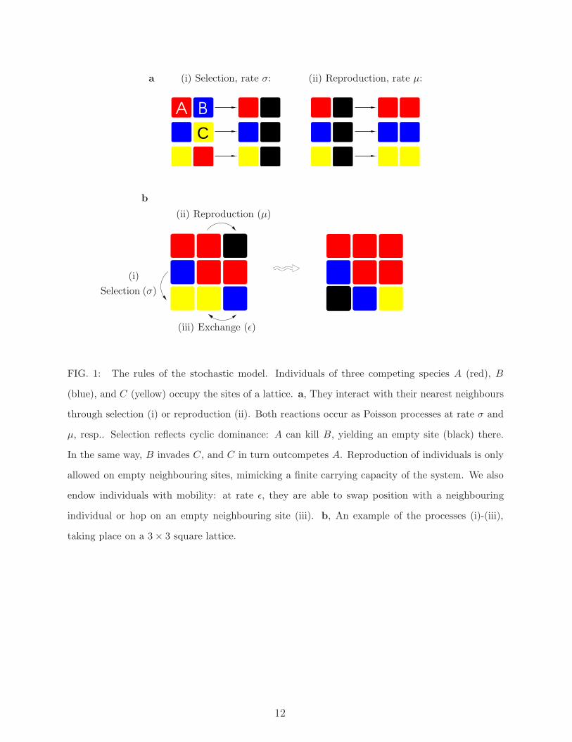
FIG. 1: The rules of the stochastic model. Individuals of three competing species A (red), B

(blue), and C (yellow) occupy the sites of a lattice. a, They interact with their nearest neighbours

through selection (i) or reproduction (ii). Both reactions occur as Poisson processes at rate σ and

µ, resp.. Selection reflects cyclic dominance: A can kill B, yielding an empty site (black) there.

In the same way, B invades C, and C in turn outcompetes A. Reproduction of individuals is only

allowed on empty neighbouring sites, mimicking a finite carrying capacity of the system. We also

endow individuals with mobility: at rate ǫ, they are able to swap position with a neighbouring

individual or hop on an empty neighbouring site (iii). b, An example of the processes (i)-(iii),

taking place on a 3 × 3 square lattice.

12

��������������������������������������������������

��������������������������������������������������a

M3 × 10−6 3 × 10−5 3 × 10−4 Mc

bbbbbb

1 × 10−51 × 10−51 × 10−51 × 10−51 × 10−51 × 10−5 1 × 10−41 × 10−41 × 10−41 × 10−41 × 10−41 × 10−4 1 × 10−31 × 10−31 × 10−31 × 10−31 × 10−31 × 10−3000000

0.20.20.20.20.20.2

0.40.40.40.40.40.4

0.60.60.60.60.60.6

0.80.80.80.80.80.8

111111

UniformityUniformityUniformityUniformityUniformityUniformity

BiodiversityBiodiversityBiodiversityBiodiversityBiodiversityBiodiversity

Extinct

ion

pro

bab

ility,

Pext

Extinct

ion

pro

bab

ility,

Pext

Extinct

ion

pro

bab

ility,

Pext

Extinct

ion

pro

bab

ility,

Pext

Extinct

ion

pro

bab

ility,

Pext

Extinct

ion

pro

bab

ility,

Pext

Mobility, MMobility, MMobility, MMobility, MMobility, MMobility, M

McMcMcMcMcMc

FIG. 2: Mobility below a critical value Mc induces biodiversity; while two species go extinct above

that threshold. a, We show snapshots obtained from lattice simulations of typical states of the

system after long evolutions (i.e. at time t ∼ N) and for different values of M (each color, blue,

yellow and red, represents one of the species and black dots indicate empty spots). Increasing

M (from left to right), the spiral structures grow, and outgrow the system size at the critical

mobility Mc: then, coexistence of all three species is lost and uniform populations remain (right).

b, Quantitatively, we have considered the extinction probability Pext that, starting with randomly

distributed individuals on a square lattice, the system has reached an absorbing state after a

waiting time t = N . We compute Pext as function of the mobility M (and σ = µ = 1), and

show results for different system sizes: N = 20 × 20 (green), N = 30 × 30 (red), N = 40 × 40

(purple), N = 100 × 100 (blue), and N = 200 × 200 (black) . As the system size increases, the

transition from stable coexistence (Pext = 0) to extinction (Pext = 1) sharpens at a critical mobility

Mc ≈ (4.5 ± 0.5) × 10−4.

13

a Typical spiral b Lattice simulations c Stochastic PDE d Deterministic PDE

λ

ω

FIG. 3: Spiralling patterns. a, Typical spiral (schematic). It rotates around the origin (white

dot) at a frequency ω and possesses a wavelength λ. b, In our lattice simulations, when the

mobility of individuals lies below the critical value, all three species coexist, forming mosaics of

entangled, rotating spirals (each color represents one of the species and black dots indicate empty

spots). c, We have found that the system’s evolution can aptly be described by stochastic partial

differential equations. In the case of lattice simulations and stochastic partial differential equations,

internal noise acts as a source of local inhomogeneities and ensures the robustness of the dynamical

behaviour: the evolution and the resulting patterns are independent of the initial conditions. d,

Ignoring the effects of noise, one is left with deterministic partial differential equations which also

give rise to spiralling structures. The latter share the same wavelength and frequency with those of

the stochastic description but, in the absence of fluctuations, their overall size and number depend

on the initial conditions and can deviate significantly from their stochastic counterparts. In b and

c, the system is initially in a homogeneous state, while d has been generated by considering an

initial local perturbation. Parameters are σ = µ = 1 and M = 1 × 10−5.

14

UniformityUniformityUniformity

BiodiversityBiodiversityBiodiversity

1 × 10−31 × 10−31 × 10−3

1 × 10−41 × 10−41 × 10−4

1 × 10−51 × 10−51 × 10−5

0.010.010.01 000 100100100

Cri

tica

lm

obility,

Mc

Cri

tica

lm

obility,

Mc

Cri

tica

lm

obility,

Mc

Reproduction rate, µReproduction rate, µReproduction rate, µ

FIG. 4: Phase diagram. The critical mobility Mc as a function of the reproduction rate µ yields

a phase diagram with a phase where biodiversity is maintained as well as a uniform one where

two species go extinct. Time unit is set by σ = 1. On the one hand, we have computed Mc

from lattice simulations, using different system sizes. The results are shown in blue (with error

bars). On the other hand, we have calculated Mc using the approach of stochastic PDE (black

dots) as well as analytically via the complex Ginzburg-Landau equation (red line). Varying the

reproduction rate, two different regimes emerge. If µ is much smaller than the selection rate, i.e.

µ ≪ σ, reproduction is the dominant limiter of the evolution. In this case, there is a linear relation

with the critical mobility, i.e. Mc ∼ µ, as follows from dimensional analysis. In the opposite case,

if reproduction occurs much faster than selection (µ ≫ σ), the latter limits the coevolution and Mc

depends linearly on σ, i.e. Mc ∼ σ. Here, as σ = 1 is kept fixed (time-scale unit), this behaviour

reflects in the fact that Mc approaches a constant value for µ ≫ σ.

15

Mobility promotes and jeopardizes biodiversity in

rock-paper-scissors games

Tobias Reichenbach, Mauro Mobilia, and Erwin Frey

Supplementary Information

In this Supplementary Information, we further elaborate our analysis by explaining some

technical aspects of the Letter and illustrate our finding by providing two supplementary

movies. The latter illustrate the spatiotemporal evolution of the biodiverse reactive states

occurring in the system under consideration.

Below, we first present the concept of extensivity, which allows to precisely discriminate

between the regime where biodiversity is stable (i.e. maintained) and the situation where

it is unstable and the system settles in one of the uniform (absorbing) states. Then, we

show how the spirals’ wavelength λ is related to the mobility M . We also explain that

such a relation has allowed to derive the functional dependence Mc(µ) of the critical

mobility on the reproduction rate. Finally, the main findings reported in the Letter are

revisited in a supplementary discussion centered on the information conveyed by the movies.

Extensivity

Even if coexistence is stable, as observed for low mobilities, there is a certain probability

that two species go extinct due to possible large yet rare fluctuations. Indeed, the only

absorbing states where no reactions (and therefore no fluctuations) occur, are the uniform

configurations where only one species survives. For this reason, these are the only stable

states in the long run. However, the typical waiting time T (N) until extinction occurs

is generally very long when the system size N is large. This suggests to consider the

dependence of the waiting time T (N) on N . Quantitatively, we discriminate between

stable and unstable coexistence by using the concept of extensivity, adapted from statistical

physics. If the ratio T/N tends to infinity (T/N → ∞) in the asymptotic limit of large

systems (N → ∞), the typical waiting time strongly prolongs with N (typically with an

exponential dependence). This scenario is called super-extensive or stable. On the other

16

hand, if T/N → O(1) (i.e. the ratio approaches a finite non-zero value) that is referred to

as the extensive case, which has been shown in11 to correspond to marginal (or neutral)

stability. Instability of the coexistence state (towards a uniform one) is encountered when

T/N → 0 (sub-extensive scenario), where the waiting time is short as compared to the

system size.

In the situations of Fig. 2, we have considered the extinction probability Pext that, starting

form random initial conditions (i.e. spatially homogeneous configurations, with equal

concentrations of each species), the system has reached a uniform state after a time t

proportional to the system size, i.e. t ∼ N . In the asymptotic limit N → ∞, three distinct

cases arise. In a first regime, the extinction probability tends to zero with the system size

N . In Fig. 2, this occurs when M < Mc. This scenario corresponds to the superextensive

situation (i.e. T/N → ∞, with N → ∞) where the coexistence of all populations is stable.

As a second case, the extinction probability approaches a finite value between 0 and 1, i.e.

T/N → O(1), and we recover neutral stability. In Fig. 2, such a behaviour arises exclusively

at the vicinity of the critical mobility Mc. In a third regime, the extinction probability does

reach the value 1, which means that T/N → 0. This is the subextensive scenario where the

coexistence is unstable and biodiversity is lost. In Fig. 2, this happens above the critical

mobility, i.e. when M > Mc.

Scaling relation and critical mobility

An important question is to understand what is the mechanism driving the transition

from a stable coexistence to extinction at the critical mobility Mc. To address this issue,

we first note that varying the mobility induces a scaling effect, as illustrated in Fig. 2. In

fact, increasing the mobility rate M results in zooming into the system. As discussed above

(see the main text and Methods), the system’s dynamics is described by a set of suitable

stochastic partial differential equations (SPDE) (T.R., M.M., and E.F., in preparation)

whose basic properties help rationalize this scaling relation. In fact, the mobility enters the

stochastic equations through a diffusive term M∆, where ∆ is the Laplace operator involving

second-order spatial derivatives. Such a term is left invariant when M is multiplied by a

factor α while the spatial coordinates are rescaled by√

α. It follows from this reasoning

that varying M into αM translates in a magnification of the system’s characteristic size

17

by a factor√

α. This implies that the spirals’ wavelength λ is proportional to√

M (i.e.

λ ∼√

M) up to the critical Mc .

When the spirals have a critical wavelength λc, associated with the mobility Mc, these

rotating patterns outgrow the system size which results in the loss of biodiversity (see the

main text). In the “natural units” (length is measured in lattice size units and the time-scale

is set by keeping σ = 1), we have numerically computed λc = 0.8 ± 0.05. This quantity has

been found to be universal, i.e. its value remains constant upon varying the rates σ and µ.

However, this is not the case of the critical mobility Mc, which depends on the parameters of

the system. Below the critical threshold Mc, the evolution is characterized by the formation

of spirals of wavelength λ(µ, M) ∼√

M . This relation, together with the universal character

of λc, leads to the following equation:

Mc(µ) =( λc

λ(µ, M)

)2

M , (2)

which gives the functional dependence of the critical mobility upon the system’s parameter.

To obtain the phase diagram reported in Fig. 4 we have used Eq. (2) together with values

of λ(µ, M) obtained from numerical simulations. For computational convenience, we have

measured λ(µ, M) by carrying out a careful analysis of the SPDE’s solutions. The results

are reported as black dots in Fig. 4. We have also confirmed these results through lattice

simulations for systems with different sizes and the results are shown as blue dots in Fig.

2. Finally, we have taken advantage of the analytical expression (up to a constant prefac-

tor, taken into account in Fig. 2) of λ(µ, M) derived from the complex Ginzburg-Landau

equation (CGLE) associated with the system’s dynamics (see Methods): with Eq. (2), we

have obtained the red curve displayed in Fig. 2. This figure corroborates the validity of the

various approaches (SPDE, lattice simulations and CGLE), which all lead to the same phase

diagram where the biodiverse and the uniform phases are identified.

Supplementary Movie 1

In the first movie, the dynamics of individuals of species A, B and C follows the reactions

illustrated in Fig. 1 with rates µ = 1 (reproduction), σ = 1 (selection) and ǫ = 2.4 (exchange

rate). In Movie 1, individuals of each species are indicated in different colours (empty sites

are shown as black dots). The evolution takes place on a square lattice of N = 400 × 400

18

sites, such that there are up to 1.6 × 105 individuals in the system. This set of parameters

corresponds to a mobility rate M = 2ǫ/N = 3 × 10−5 well below the critical threshold

Mc ≈ 4.5 ± 0.5 × 10−4 (see Figs. 2, 4 and text). Initially the system is in a well-mixed

configuration with equal density of individuals of each species and empty sites. As time

increases and since M < Mc, biodiversity is maintained and complex dynamical patterns

form in the course of the evolution resulting in a rich entanglement of spiral waves.

Supplementary Movie 2

In the second movie, the mobility of the individuals has been increased. In fact, the

dynamics of individuals of species still follows the reactions illustrated in Fig. 1 with rates

µ = 1 (reproduction) and σ = 1 (selection), but the exchange rate is now ǫ = 6. In Movie 2,

individuals of each species are still indicated in different colours (empty sites are shown as

black dots). The evolution takes place on a square lattice of N = 200×200 sites, allowing up

to 4 × 104 individuals in the system. This set of parameters corresponds to a mobility rate

M = 3 × 10−4 relatively close to the critical threshold Mc ≈ 4.5± 0.5 × 10−4 (see Figs. 2, 4

and text). Initially the system is in a well-mixed state with equal density of individuals

of each species and empty sites. As time increases and since M < Mc, biodiversity is still

maintained and patterns form in the course of the evolution. However, as compared to

the first movie, one notices that the size of the patterns has increased and one now only

distinguishes one pair of antirotating spirals.

19

Supplementary Discussion

The supplementary movies illustrate the system’s evolution in the coexistence phase, i.e.

the emergence of dynamical complex patterns deep in that phase (Movie 1) and close to

(yet below) the threshold Mc (Movie 2, see text and Fig. 3).

Starting from initially homogeneous (well-mixed) configurations, after a short transient

regime, spiral waves rapidly emerge and characterize the long-time behaviour of the sys-

tem which settles in a reactive steady state (super-extensive case, see text). The wavefronts,

merging to form entanglement of spirals, propagate with spreading speed v∗ and wavelength

λ. In Movies 1 and 2, it appears clearly that by rising the individuals’ mobility, one increases

the wavefronts propagation velocity and the wavelength of the resulting dynamical patterns,

as well as the size of each spiral. From PDE associated with the system’s dynamics, we can

rationalize this discussion and estimate these quantities for the cases illustrated in Movies

1 and 2. Namely, for the spreading speed, we have obtained v∗ ≈ 3.5 × 10−3 (lattice-size

units per time-step, Movie 1) and v∗ ≈ 1.1×10−2 (Movie 2). Similarly, the wavelength were

found to be λ ≈ 0.21 (lattice-size units, Movie 1) and λ ≈ 0.65 (Movie 2). Here, rising the

rate M from 3 × 10−5 (Movie 1) to 3 × 10−4 (Movie 2) results in the enhancement of v∗

and λ by a factor√

10 ≈ 3.16. In Movie 2, the size of the spirals can also be estimated to

have been magnified by the same factor√

10 ≈ 3.16 with respect to those of Movie 1. As

explained in the text, this scaling property of the system can be understood by considering

the stochastic partial differential equation describing the dynamics, which were obtained

from the underlying master equation through a system size expansion (see Methods).

By rising the individuals’ mobility, one therefore increases the size of the spiralling patterns

(whose wavelength is proportional to√

M) and for sufficiently large value of the exchange

rate (i.e. of M), as in Movie 2, just a few spirals nearly cover the entire lattice. This happens

up to the critical value λc ≈ 0.8, found to be universal. In fact, when λ ≥ λc the whole

system is covered with one single (“giant”) spiral which cannot fit within the lattice. This

effectively results in the extinction of two species and the loss of biodiversity. As explained

in the text, by exploiting the fact that λ ∝√

M and the universal character of λc, one can

infer the existence of the critical mobility rate Mc = Mc(µ) [see Eq. (2)], as illustrated in

Fig. 4. This allows to discuss the fate of the system (i.e. biodiversity versus extinction) in

terms of the reaction and mobility rates µ and M , respectively: For given reaction rates µ

20

and ǫ (without loss of generality σ is set to unity, see text) and system size L, we obtain

a critical value Mc(µ) of the mobility rate. In fact, a reactive steady state is reached (and

biodiversity maintained) only if M < Mc(µ). When the individuals’ mobility is too fast,

i.e. when M > Mc(µ), the system can be considered to be well-mixed and its dynamics

therefore can be aptly described in terms of homogeneous rate equations which predicts the

extinction of two species (see Methods).

In the cases illustrated in Movies 1 and 2, Mc ≈ 4.5 ± 0.5 × 10−4 and the wavefronts prop-

agate with λ < λc, so that biodiversity is always preserved. However, we notice that the

resulting spatiotemporal patterns are quite different: while one finds a rich entanglement of

spirals deep in the coexistence phase (i.e. for M ≈ 3 × 10−5 ≪ Mc, Movie 1), only one pair

of antirotating spirals fill the system when one approaches the critical value Mc (Movie 2).

21