LUND UNIVERSITY

PO Box 117221 00 Lund+46 46-222 00 00

Tobit Maximum-likelihood estimation of Censored Pathloss Data

Gustafson, Carl; Abbas, Taimoor; Bolin, David; Tufvesson, Fredrik

Published: 2015-01-01

Link to publication

Citation for published version (APA):Gustafson, C., Abbas, T., Bolin, D., & Tufvesson, F. (2015). Tobit Maximum-likelihood estimation of CensoredPathloss Data. (Technical report, Dept. of Electrical and Information Technology, Lund University, Sweden).[Publisher information missing].

General rightsCopyright and moral rights for the publications made accessible in the public portal are retained by the authorsand/or other copyright owners and it is a condition of accessing publications that users recognise and abide by thelegal requirements associated with these rights.

• Users may download and print one copy of any publication from the public portal for the purpose of privatestudy or research. • You may not further distribute the material or use it for any profit-making activity or commercial gain • You may freely distribute the URL identifying the publication in the public portalTake down policyIf you believe that this document breaches copyright please contact us providing details, and we will removeaccess to the work immediately and investigate your claim.

Download date: 04. Jun. 2018

1

Tobit Maximum-likelihood estimation of CensoredPathloss Data

Carl Gustafson, Taimoor Abbas, David Bolin and Fredrik Tufvesson

Abstract—Pathloss is typically modeled using a log-distancepower law with a large-scale fading term that is log-normal.However, the received signal is affected by the dynamic rangeand noise floor of the measurement system used to sound thechannel, which can cause measurement samples to be truncatedor censored. If the information about the censored samples arenot included in the estimation method, as in ordinary leastsquares estimation, it can result in biased estimation of both thepathloss exponent and the large scale fading. This is solved byapplying a Tobit maximum-likelihood estimator, which providesconsistent estimates for the pathloss parameters. This technicalreport provides information about the Tobit maximum-likelihoodestimator estimator and its asymptotic variance under certainconditions.

Keywords—Pathloss, maximum-likelihood estimation, ordinaryleast squares, censored data, truncated data, vehicular communi-cation.

I. INTRODUCTION

Pathloss describes the expected loss in received power asa function of the transmitter (Tx) and receiver (Rx) separa-tion distance and the effects of random large scale fading.It includes losses due to the expansion of the radio wavefront in space as well as losses due to reflection, scattering,diffraction and penetration. A number of pathloss modelshave been developed for a variety of wireless communicationsystems, e.g., cellular systems, Bluetooth, Wi-Fi, vehicle-to-vehicle communications, and, mm-wave point-to-point com-munications, operating over different frequency bands rangingfrom hundreds of MHz to tens of GHz [1]–[4]. These modelshave widely been used for the prediction and simulation ofsignal strengths for given Tx-Rx separation distances. Pathlossmodels are often developed based on channel measurements inrealistic user scenarios. The model parameters estimated frommeasurement data are thus typically valid only for a particularfrequency range, antenna arrangement, and environment forthe targeted user scenario.

However, in practice, the observation of the received signalpower at the receiver is limited by the system noise, i.e., thesignals with power below the noise floor can not be measuredproperly. In many vehicle-to-vehicle measurements, this limi-tation due to the system noise is often present at longer dis-tances [5]–[7]. Also, in mm-wave measurements, the pathloss

This work was supported by the VINNOVA FFI program Wireless Com-munications in Automitve Environments.

C. Gustafson and F. Tufvesson are with the Dept. of Electrical andInformation Technology, Lund University, Sweden.

T. Abbas is with the Volvo Car Corporation, Gothenburg, Sweden.D. Bolin is with the Mathematical Sciences, Chalmers University of

Technology, Gothenburg, Sweden.

values are in general larger than at lower frequencies, whicheffectively can reduce the range in which the data is unaffectedby the noise floor. Due to the limited dynamic range of themeasurement system, sample data might be truncated, wherebyall data above or below a certain range are immeasurable,or censored, meaning that all data above or below a certainrange are counted, but not measured. Estimation of the clusterdecay and cluster fading based on truncated data has previouslybeen addressed in [8]. For clusters, the data is modeled astruncated, since it is generally impossible to measure or countclusters that are below the noise floor. However, in pathlossmeasurements, since the distances where the received powerfalls below the noise floor are known, it is possible to modelthe data as being censored. Estimating statistical parameterswithout considering the effects of censored or truncated datasamples, can lead to erroneous results. The fact that thiscan be a problem for pathloss data is acknowledged in [6],however, the authors do not give any detailed information onhow to solve this issue. In this technical report, we discussthe use of a Tobit model [9] for censored pathloss data anda maximum-likelihood (ML) method for the estimation ofpathloss parameters [10].

II. PATHLOSS MODELING

Path loss is often modeled by a log-distance power law plusa large scale fading term [11]. In units of dB this can be writtenas

PL(d) = PL(d0) + 10nlog10

(d

d0

)+ Ψσ, d ≥ d0, (1)

where d is the distance, n is the pathloss exponent, PL(d0)is the pathloss at a reference distance of d0 and Ψσ is arandom variable that describes the large-scale fading about thedistance-dependent mean pathloss. For measurement data, it ishere assumed that the effects of small scale fading is removedfrom the data set. It is also assumed that the peak value of theaggregated antenna gain is removed from the measurementdata [12]. Ideally, the variation of the aggregated antennagain should be small, so that it does not affect the measuredlarge-scale fading too much. The large-scale fading term isusually modeled by a log-normal distribution, which in the dB-domain corresponds to a zero-mean Gaussian distribution withstandard deviation σ, i.e., Ψσ ∼ N (0, σ2). Hence, the pathlossis normally distributed with a distance dependent expectedvalue, PL(d) ∼ N (µ(d), σ2), where

µ(d) = PL(d0) + 10nlog10

(d

d0

). (2)

2

The reference value PL(d0) can be estimated based onmeasurement data, or based on reference measurements at thisdistance. For line-of-sight (LOS) scenarios, it is sometimesdeterministically modeled based on the free-space pathloss, as

PL(d0) = 20log10

(4πd0λ

). (3)

Here λ is the wavelength at the given frequency. Here, itis worth noting that the approach of using the deterministicreference value of Eq. (3) only provides theoretically correctresults if the pathloss exponent is equal to 2. If the pathlossexponent is not equal to 2, but Eq. (3) is used to determine thereference value, the data model of Eq. 1 is inconsistent, as itdepends on the choice of the reference distance d0. For non-line-of-sight (NLOS) scenarios, it is clear that the free-spaceequation (3) does not hold, which means that the referencevalue in this case must be determined in another fashion. Dueto the above, it is preferable to use actual measurements of thereference level, or, to estimate it based on the measurementdata. In some cases, it might be difficult to produce reliablemeasurements of the reference value scenarios due to practicalreasons, especially considering that it might be hard to producea large number of uncorrelated measurement samples exactlyat d0.

III. ESTIMATION BY ORDINARY LEAST SQUARES

To completely model the pathloss and large-scale fading fora given data set, we wish to estimate the three parametersof (1), i.e., n, PL(d0) and σ2. The data under considerationis implicitly assumed to be Gaussian since Ψσ is Gaussianin the dB domain. Using (1) the data set for L path lossmeasurements can be written as,

y = Xα + ε, (4)

wherey = [PL(d/d0)]L×1 ,

X = [1 10log10(d/d0)]L×2,

α = [PL(d0) n]T .

(5)

The term ε = [Ψσ]L×1 is a row vector describing the large-scale fading term for each of the L different pathloss samples.

When there are no censored samples, the parameters of thelog-distance power law can be estimated by applying ordinaryleast squares (OLS). The parameter α is then estimated as1

α =(XTX

)−1XTy. (6)

The variance of the large-scale fading, σ2, can then be esti-mated as

σ2 =1

L− 1(y −Xα)T (y −Xα). (7)

1As the variance σ2 is assumed to be independent of delay, weighted leastsquares (WLS) are not applied. However, we note that WLS could be of usefor cases when σ2 is being modeled with a distance dependence.

The estimate α is Gaussian,

αj ∼ N(αj , σ

2(XTX)−1jj), j = 1, 2, (8)

which alternatively can be expressed as

PL(d0) = α1 ∼ N(PL(d0), σ2

(L−1 + x2S−1xx

)),

n = α2 ∼ N(n, σ2S−1xx

),

(9)

where

x =1

L

L∑l=1

10log10(dl/d0),

Sxx =

L∑l=1

(10log10(dl/d0)− x)2.

(10)

Using Eq. (9), standard errors2 for n and PL(d0) can be foundby replacing the unknown standard deviation of the large scalefading, σ, by its estimate, σ, which gives

SE(n) = σ√S−1xx ,

SE(PL(d0)) = σ√L−1 + x2S−1xx .

(11)

The standard errors are useful for evaluating the accuracyof the estimated parameters. However, it should be stressedthat these standard errors only applies when the data actuallyfollows the log-distance power law model with a large-scalefading variance that is independent of delay. For this reason, itis often necessary to validate the measurement data againstthe presumed model. This could be done by investigatingthe residuals between the measured data and the regression,to make sure that the residuals do not exhibit any sort ofdistance dependence. If the data seems to be described by adifferent model, then a different pathloss model would have tobe considered. The standard error of the parameters estimatedwith OLS depend on the number of samples and the exactpathloss sample distances that are used in the measurement.However, if the data is being censored, OLS would providebiased results, which means that Eq. (11) no longer applies.

IV. ESTIMATION OF CENSORED PATHLOSS DATA

In order to estimate the pathloss exponent and fadingvariance of censored data, with a known number of missingsamples where only the distance is known, it is possible tobase the estimation on a censored normal distribution. Underthis assumption, the observations follow a censored normaldistribution [9]. The censoring occurs for data samples wherethe pathloss is greater than or equal to c. The value −c isa channel gain that corresponds to the noise floor of thechannel sounder or measurement device. In practice, c ischosen with some margin with respect to the noise floor, so thata limited number of samples dominated by noise are includedas measurement data. Using the data set model in (4), the datais assumed to be censored so that observations with values ator above c are set to c, i.e.,

2The standard error is the standard deviation of the sampling distributionof a statistic.

3

yi =

{y∗i if y∗i < cc if y∗i ≥ c

(12)

where

y∗i ∼ N (xiα, σ2). (13)

The probability of observing a censored observation at adistance d is given by

P (y ≥ c) = 1− Φ

(c− xiα

σ

), (14)

where Φ is the cumulative distribution function (CDF) of thestandard normal distribution. Now, by using I as an indicatorfunction that is set to 1 if the observation is uncensored andis set to 0 if the observation is censored, it is possible to writedown the likelihood function as [9]

l(σ,α) =

N∏i=1

[1

σφ

(yi − xiα

σ

)]Ii [1− Φ

(c− xiα

σ

)]1−Ii,

where φ is the standard normal probability density function(PDF). The log-likelihood L(σ,α) = ln[l(σ,α)] can now bewritten as

L(σ,α) =

N∑i=1

Ii

[−lnσ + lnφ

(yi − xiα

σ

)]

+

N∑i=1

(1− Ii)ln[1− Φ

(c− xiα

σ

)].

(15)

Using the log-likelihood, the parameters σ and α are estimatedusing

[σ, α] = arg minσ,α

{−L(σ,α)}, (16)

which is easily solved by numerical optimization of α andσ, using for instance the method of Newton [10]. In thiswork, we have solved this by using the fminsearch function inMatlab, which is based on a Nelder-Mead search method. Theestimates obtained from OLS were used as initial values forthe minimization. The presented method approach can easilybe further extended, so that it supports other pathloss models.

A. Asymptotic Variance of the ML estimatorThe asymptotic variance of the ML estimator has been

derived in [10] for the problem with censoring of sampleswhere yi ≤ 0. We therefore transform the data in Eq. (4), byletting

yt = −y + c = −Xα− ε + c = Xαt − ε, (17)

whereαt = [−PL(d0) + c − n]T . (18)

The parameters to be estimated for the transformed data are

θt = [αTt σ2]T . (19)

The asymptotic variance for the ML estimates of the originalparameters, θ, are however the same as for the parameters ofthe transformed data, θt. Therefore, we can directly use theequations found in [10] to calculate the asymptotic varianceas

Avar(θ) = Avar(θt) = diag

(

N∑i=1

Ai(xi,θt)

)−1 , (20)

whereAi(Xi,θt) =

(aix

Ti xi bix

Ti

bixi ci

), (21)

with coefficients

ai = −σ−2[ziφi − φ2i /(1− Φi)− Φi

],

bi = σ−3[z2i φi + φi − ziφ2i /(1− Φi)

]/2,

ci = −σ−4[z3i φi + ziφi − z2i φ2i /(1− Φi)− 2Φi

]/4.

(22)

Here, φi = φi(zi) and Φi = Φi(zi) and zi = xiαt/σ. In orderto avoid numerical issues when calculating the coefficients inEq. 22, it is worthwhile to rewrite the ratio φi/(1− Φi) as

φi(zi)

1− Φi(zi)=

1√2π

exp(−z2i /2)

1− 12erfc(−zi/

√2)

=2√

2πerfcx(zi/√

2), (23)

where erfc(·) is the complementary error function and erfcx(·)is the scaled complementary error function.

As stated previously, the asymptotic variances of the pa-rameters θt are the same as for θ. Therefore, the asymptoticvariance of the parameters PL(d0), n and σ2 are given bythe three main diagonal elements of the matrix in Eq. (20).For measurement data, an estimate of the asymptotic variancecan be found by replacing the true parameter values with theirestimates, PL(d0), n and σ2. Estimates of the standard errorscan then be obtained simply by taking the square root of theasymptotic variance.

The standard errors of the estimated parameters depend onmany different things, such as the pathloss sample distances,the level of the censoring, the number of samples as well asthe exact values of PL(d0), n and σ2. Therefore, it is oftennecessary to evaluate the standard errors for each individualmeasurement case. In order to give an illustrative example,Fig. 1 shows the standard errors calculated for syntheticpathloss data with known parameters, that is sampled at equallyspaced distances on a linear scale, starting from 1 m. The thicklines are the standard errors for pathloss data that is censoredat a level of 90 dB, whereas the thin lines are for data that iscompletely uncensored. The dashed line indicates the distanceat which the expected value of the pathloss is equal to thecensoring level. As the distance is increased, the standard errorfor the case with censoring starts to deviate from the case withno censoring, just as expected. This deviation seems to beespecially severe for the large scale fading variance. However,for n and PL(d0), the standard errors are fairly similar forthe two cases even for distances beyond the point where thepathloss starts to fall below the censoring level. Fig. 2 showsvirtually the same thing as Fig. 1, except that the distance issampled using equally spaced distances on a logarithmic scale.

4

101 102 103100

101

102

103

Dis

tanc

e[m

]Standard error of PL(d0)

0.50.7511.251.5

101 102 103100

101

102

103

Dis

tanc

e[m

]

Standard error of n

0.10.20.30.40.5

101 102 103100

101

102

103

Number of pathloss samples, N

Dis

tanc

e[m

]

Standard error of σ2

12345

Fig. 1. Standard errors for pathloss parameters estimated with the MLestimator. The true values of the parameters are PL(d0) = 47.9 dB, n = 2and σ = 4. The thick lines are standard errors for data that is censored at alevel corresponding to pathloss values of 90 dB, whereas the thin lines are fordata that is completely uncensored (which corresponds to the standard errorsof OLS). The dashed lines indicate the distance at which the expected valueof the pathloss is equal to the censoring level. The data is sampled at equallyspaced distances on a linear scale, starting from 1 m.

This shows that logarithmically spaced measurement distancesrequires fewer samples, compared to linearly spaced distances,in order to reach the same standard error for the estimatedparameters.

101 102 103100

101

102

103

Dis

tanc

e[m

]

Standard error of PL(d0)

0.50.75

11.251.5

101 102 103100

101

102

103

Dis

tanc

e[m

]

Standard error of n

0.10.20.30.40.5

101 102 103100

101

102

103

Number of pathloss samples, N .

Dis

tanc

e[m

]

Standard error of σ2

12345

Fig. 2. Standard errors for pathloss parameters estimated with the MLestimator, with the same conditions as in Fig. 2, except that the data is sampledat equally spaced distances on a logarithmic scale, starting from 1 m.

V. RESULTS

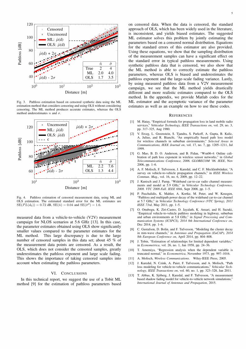
As an example, synthetic data at 5.6 GHz was generatedaccording to Eq. (1) with known parameters (n = 2 andσ = 4) and a synthetic censoring level at c. The parameterswere estimated using OLS and the ML method describedabove. The result is shown in Fig. 3. The OLS method clearlyunderestimates both the pathloss exponent, n, as well as thestandard deviation of the large scale fading, σ. The ML methodon the other hand, is able to correctly estimate both parametersin this example. Fig. 4 shows the same thing as Fig. 3, but is for

5

100 101 102 103

40

60

80

100

120

µ(d) + 2σ

µ(d) - 2σ

Distance [m]

Path

loss

[dB

]

CensoredUncensoredML: µ(d)OLS: µ(d)

n σTrue 2 4ML 2.0 4.0

OLS 1.7 3.5

Fig. 3. Pathloss estimation based on censored synthetic data using the MLestimation method that considers censoring and using OLS without consideringcensoring. The ML method produces accurate estimates, whereas the OLSmethod underestimates n and σ.

101 102 103

60

80

100

120 µ(d) + 2σ

µ(d) - 2σ

Distance [m]

Path

loss

[dB

]

UncensoredML: µ(d)OLS: µ(d)c

n σML 2.2 7.6

OLS 1.3 4.4

Fig. 4. Pathloss estimation of censored measurement data, using ML andOLS estimation. The estimated standard error for the ML estimates areSE(PL(d0)) = 0.72 dB, SE(n) = 0.04 and SE(σ2) = 1.6.

measured data from a vehicle-to-vehicle (V2V) measurementcampaign for NLOS scenarios at 5.6 GHz [13]. In this case,the parameter estimates obtained using OLS show significantlysmaller values compared to the parameter estimates for theML method. This large discrepancy is due to the largenumber of censored samples in this data set; about 45 % ofthe measurement data points are censored. As a result, theOLS, which does not consider the censored samples, greatlyunderestimates the pathloss exponent and large scale fading.This shows the importance of taking censored samples intoaccount when estimating the pathloss parameters.

VI. CONCLUSIONS

In this technical report, we suggest the use of a Tobit MLmethod [9] for the estimation of pathloss parameters based

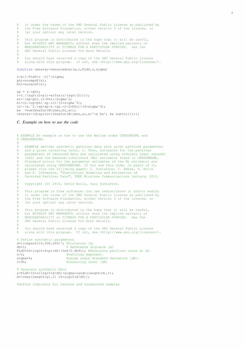
on censored data. When the data is censored, the standardapproach of OLS, which has been widely used in the literature,is inconsistent, and yields biased estimates. The suggestedML estimator solves this problem by jointly estimating theparameters based on a censored normal distribution. Equationsfor the standard errors of this estimator are also provided.Using these equations, we show that the sampling distributionof the measurement samples can have a significant effect onthe standard error in typical pathloss measurements. Usingsynthetic pathloss data that is censored, we also show thatthe ML method is able to correctly estimate the pathlossparameters, whereas OLS is biased and underestimates thepathloss exponent and the large-scale fading variance. Lastly,by using measured pathloss data from a V2V measurementcampaign, we see that the ML method yields drasticallydifferent and more realistic estimates compared to the OLSmethod. In the appendix, we provide Matlab codes for theML estimator and the asymptotic variance of the parameterestimates as well as an example on how to use these codes.

REFERENCES

[1] M. Hatay, “Empirical formula for propagation loss in land mobile radioservices,” Vehicular Technology, IEEE Transactions on, vol. 29, no. 3,pp. 317–325, Aug 1980.

[2] V. Erceg, L. Greenstein, S. Tjandra, S. Parkoff, A. Gupta, B. Kulic,A. Julius, and R. Bianchi, “An empirically based path loss modelfor wireless channels in suburban environments,” Selected Areas inCommunications, IEEE Journal on, vol. 17, no. 7, pp. 1205–1211, Jul1999.

[3] G. Mao, B. D. O. Anderson, and B. Fidan, “Wsn06-4: Online cali-bration of path loss exponent in wireless sensor networks,” in GlobalTelecommunications Conference, 2006. GLOBECOM ’06. IEEE, Nov2006, pp. 1–6.

[4] A. F. Molisch, F. Tufvesson, J. Karedal, and C. F. Mecklenbrauker, “Asurvey on vehicle-to-vehicle propagation channels,” in IEEE WirelessCommun. Mag., vol. 16, no. 6, 2009, pp. 12–22.

[5] J. Kunisch and J. Pamp, “Wideband car-to-car radio channel measure-ments and model at 5.9 GHz,” in Vehicular Technology Conference,2008. VTC 2008-Fall. IEEE 68th, Sept 2008, pp. 1–5.

[6] P. Paschalidis, K. Mahler, A. Kortke, M. Peter, and W. Keusgen,“Pathloss and multipath power decay of the wideband car-to-car channelat 5.7 GHz,” in Vehicular Technology Conference (VTC Spring), 2011IEEE 73rd, May 2011, pp. 1–5.

[7] O. Onubogu, K. Ziri-Castro, D. Jayalath, K. Ansari, and H. Suzuki,“Empirical vehicle-to-vehicle pathloss modeling in highway, suburbanand urban environments at 5.8 GHz,” in Signal Processing and Com-munication Systems (ICSPCS), 2014 8th International Conference on,Dec 2014, pp. 1–6.

[8] C. Gustafson, D. Bolin, and F. Tufvesson, “Modeling the cluster decayin mm-wave channels,” in Antennas and Propagation (EuCAP), 20148th European Conference on, April 2014, pp. 804–808.

[9] J. Tobin, “Estimation of relationships for limited dependent variables,”in Econometrica, vol. 26, no. 1, Jan 1958, pp. 24–36.

[10] T. Amemiya, “Regression analysis when the dependent variable istruncated normal,” in Econometrica, November 1973, pp. 997–1016.

[11] A. Molisch, Wireless Communications. Wiley-IEEE Press, 2005.[12] J. Karedal, N. Czink, A. Paier, F. Tufvesson, and A. Molisch, “Path

loss modeling for vehicle-to-vehicle communications,” Vehicular Tech-nology, IEEE Transactions on, vol. 60, no. 1, pp. 323–328, Jan 2011.

[13] T. Abbas, K. Sjoberg, J. Karedal, and F. Tufvesson, “A measurementbased shadow fading model for vehicle-to-vehicle network simulations,”International Journal of Antennas and Propagation, 2015.

6

APPENDIX

A. Maximum-likelihood estimator

% CENSOREDML Numerical maximum-likelihood estimation of a censored normal% distribtuion.%% CENSOREDML(X,Y,C,T,A,S2) performs a numerical optimization of the parameters% for the log-likelihood of a censored normal distribution.% The data is assumed to be of the form Y=alpha*X+e, where alpha are regression% coefficients and e is r.v. that is Gaussian with zero mean.%% C is a constant describing the censoring level and T is a vector indicating if% the samples are censored or uncensored (0 indicates that the sample is% censored and 1 indicates that it is uncensored). A and S are initial values for% the regression parameters and the variance of the error, respectively.% For pathloss estimation, A contains the initial values of [PL(d0); n] and S is% the initial value of the large scale fading variance sigma2. If You use this% code, or parts of it, please cite the following paper:% C. Gustafson, T. Abbas, D. Bolin and F. Tufvesson,% "Statistical Modeling and Estimation of Censored Pathloss Data",% IEEE Wireless Communications Letters, 2015.%% Copyright (C) 2015, David Bolin, Carl Gustafson.%% This program is free software: you can redistribute it and/or modify% it under the terms of the GNU General Public License as published by% the Free Software Foundation, either version 3 of the License, or% (at your option) any later version.%% This program is distributed in the hope that it will be useful,% but WITHOUT ANY WARRANTY; without even the implied warranty of% MERCHANTABILITY or FITNESS FOR A PARTICULAR PURPOSE. See the% GNU General Public License for more details.%% You should have received a copy of the GNU General Public License% along with this program. If not, see <http://www.gnu.org/licenses/>.

function est=censoredml(x,y,c,t,a_est,s2e)

opts = optimset('GradObj','off', 'Largescale','off','MaxFunEvals',20000);pars = fminsearch(@(pars) censoredllh(pars),[a_est;log(s2e)],opts);est=[pars(1:2); sqrt(exp(pars(3)))];

function l = censoredllh(p)L = zeros(size(y));L(t==1)=-0.5*(y(t==1)-x(t==1,:)*p(1:2)).ˆ2/exp(p(3))-log(sqrt(2*pi))-p(3)/2;L(t==0)=log(1-normcdf((c-x(t==0,:)*p(1:2))/exp(p(3)/2)));l = -sum(L);

endend

B. Asymptotic Variance

% CENSOREDVAR Computes the theoretical asymptotic variance for% the estimates of the censored ML estimator.%% CENSOREDVAR(X,C,PLd0,N,SIGMA) uses the equations from T. Amemiya,% "Regression Analysis when the dependent variable is truncated normal",% Econometrica, 1987. C is the censoring level, PLd0, N and SIGMA are% either true or estimated pathloss parameter values. If You use this% code, or parts of it, please cite the following paper:% C. Gustafson, T. Abbas, D. Bolin and F. Tufvesson,% "Statistical Modeling and Estimation of Censored Pathloss Data",% IEEE Wireless Communications Letters, 2015.%% Copyright (C) 2015, David Bolin, Carl Gustafson.%% This program is free software: you can redistribute it and/or modify

7

% it under the terms of the GNU General Public License as published by% the Free Software Foundation, either version 3 of the License, or% (at your option) any later version.%% This program is distributed in the hope that it will be useful,% but WITHOUT ANY WARRANTY; without even the implied warranty of% MERCHANTABILITY or FITNESS FOR A PARTICULAR PURPOSE. See the% GNU General Public License for more details.%% You should have received a copy of the GNU General Public License% along with this program. If not, see <http://www.gnu.org/licenses/>.

function censvar=censoredvar(x,c,PLd0,n,sigma)

z=x*[-PLd0+c -n]'/sigma;phi=normpdf(z);Phi=normcdf(z);

zp = z.*phi;r=2./(sqrt(2*pi)*erfcx(z/(sqrt(2))));ai=-(zp-phi.*r-Phi)/sigmaˆ2;bi=(z.*zp+phi-zp.*r)/(2*sigmaˆ3);ci=-(z.ˆ2.*zp+zp-z.*zp.*r-2*Phi)/(4*sigmaˆ4);bx =sum(bsxfun(@times,bi,x));censvar=(diag(inv([bsxfun(@times,ai,x)'*x bx'; bx sum(ci)])));

C. Example on how to use the code

% EXAMPLE An example on how to use the Matlab codes CENSOREDML and% CENSOREDVAR.%% EXAMPLE defines synthetic pathloss data with given pathloss parameters% and a given censoring level, c. Then, estimates for the pathloss% parameters of censored data are calculated using ordinary least squares% (OLS) and the maximum-likelihood (ML) estimator found in CENSOREDML.% Standard errors for the parameter estimates of the ML estimator are% calculated using CENSOREDVAR. If You use this code, or parts of it,% please cite the following paper: C. Gustafson, T. Abbas, D. Bolin% and F. Tufvesson, "Statistical Modeling and Estimation of% Censored Pathloss Data", IEEE Wireless Communications Letters, 2015.%% Copyright (C) 2015, David Bolin, Carl Gustafson.%% This program is free software: you can redistribute it and/or modify% it under the terms of the GNU General Public License as published by% the Free Software Foundation, either version 3 of the License, or% (at your option) any later version.%% This program is distributed in the hope that it will be useful,% but WITHOUT ANY WARRANTY; without even the implied warranty of% MERCHANTABILITY or FITNESS FOR A PARTICULAR PURPOSE. See the% GNU General Public License for more details.%% You should have received a copy of the GNU General Public License% along with this program. If not, see <http://www.gnu.org/licenses/>.

% Define synthetic parametersd=linspace(10,200,200)'; %Distances [m]d0=1; % Reference distance [m]PLd0=20*log10(4*pi*d0/(3e8/5.9e9)); %Reference pathloss value at d0.n=2; %Pathloss exponent.sigma=4; %Large scale standard deviation [dB].c=90; %Censoring level [dB]

% Generate synthetic datay=PLd0+10*n*log10(d/d0)+sigma*randn(length(d),1);x=[ones(length(y),1) 10*log10(d/d0)];

%Define indicator for censore and uncensored samples

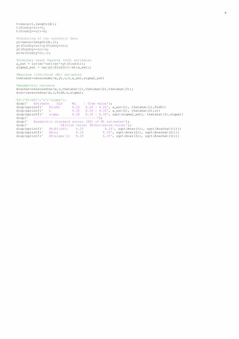
8

t=zeros(1,length(d));t(find(y<c))=1;t(find(y>=c))=0;

%Censoring of the synthetic datayt=zeros(length(d),1);yt(find(y<c))=y(find(y<c));yt(find(y>=c))=c;xt=x(find(y<c),:);

%Ordinary Least Squares (OLS) estimatesa_est = inv(xt'*xt)*xt'*yt(find(t));sigma2_est = var(yt(find(t))-xt*a_est);

%Maximum likelihood (ML) estimatesthetahat=censoredml(x,yt,c,t,a_est,sigma2_est)

%Asymptotic varianceAvarhat=censoredvar(x,c,thetahat(1),thetahat(2),thetahat(3));Avar=censoredvar(x,c,PLd0,n,sigma);

%S=['PL(d0)';'n';'sigma'];disp(' Estimate OLS ML | True value');disp(sprintf(' PL(d0) %.2f %.2f | %.2f', a_est(1), thetahat(1),PLd0))disp(sprintf(' n %.3f %.3f | %.3f', a_est(2), thetahat(2),n))disp(sprintf(' sigma %.3f %.3f | %.3f', sqrt(sigma2_est), thetahat(3),sigma))disp(' ---------------------------------');disp(' Asymptotic standard errors (SE) of ML estimates');disp(' SE(true value) SE(estimated value)');disp(sprintf(' SE(PL(d0)) %.2f %.2f', sqrt(Avar(1)), sqrt(Avarhat(1))))disp(sprintf(' SE(n) %.3f %.3f', sqrt(Avar(2)), sqrt(Avarhat(2))))disp(sprintf(' SE(sigmaˆ2) %.3f %.3f', sqrt(Avar(3)), sqrt(Avarhat(3))))