tobit models: a survey - abdelaziz benkhalifa · tobit models: a survey takeshi amemiya* stanford...
TRANSCRIPT

Journal of Econometrics 24 (1984) 3-61. North-Holland
TOBIT MODELS: A SURVEY
Takeshi AMEMIYA*
Stanford University, Stanford, CA 94305, USA
1. Introduction
Tobit models refer to regression models in which the range of the dependent variable is constrained in some way. In economics, such a model was first suggested in a pioneering work by Tobin (1958). He analyzed household expenditure on durable goods using a regression model which specifically took account of the fact that the expenditure (the dependent variable of his regression model) cannot be negative. Tobin called his model the model of limited dependent variables. It and its various generalizations are known popularly among economists as Tobit models, a phrase coined by Goldberger (1964) because of similarities to probit models. These models are also known as censored or truncated regression models. The model is called truncated if the observations outside a specified range are totally lost and censored if one can at least observe the exogenous variables. A more precise definition will be given later.
Censored and truncated regression models have been developed in other disciplines (notably biometrics and engineering) more or less independently of their development in econometrics. Biometricians use the model to analyze the survival time of a patient. Censoring or truncation occurs either if a patient is still alive at the last observation date or if he or she cannot be located. Similarly, engineers use the model to analyze the time to failure of material or of a machine or a system. These models are called survival models.’ Sociologists and economists have also used survival models to analyse the duration of such phenomena as unemployment, welfare receipt, employment in a particular job, residing in a particular region, marriage, and the period of time between
*This research was supported by a National Institute of Justice Grant no. 81-IJ-CX-0055 to Rhodes Associates. The author is grateful to Jeanne E. Anderson, A. Cohn Cameron, Aaron Han, Yoonbai Kim, Lung-Fei Lee, Thomas E. MaCurdy, Frederick C. Nold, and Dale J. Poirier for helpful suggestions.
‘See Kalbfleisch and Prentice (1980) and Miller (1981).
0304~4076/84/$3.0001984, Elsevier Science Publishers B.V. (North-Holland)

4 T. Amemiya, Tobit models: A sutvey
births.* Mathematically, survival models belong to the same general class of models as Tobit models and share certain characteristics. However, I will not discuss survival models in this survey because they possess special features of their own. See the survey by Heckman and Singer in this issue.
Between 1958, when Tobin’s article appeared, and 1970, the Tobit model was used infrequently in econometric applications, but since the early 1970’s numerous applications ranging over a wide area of economics have appeared and continue to appear. This phenomenon is due to a recent increase in the availability of micro sample survey data which the Tobit model analyzes well and to a recent advance in computer technology which has made estimation of large-scale Tobit models feasible. At the same time, many generalizations of the Tobit model and various estimation methods for these models have been proposed. In fact, models and estimation methods are now so numerous and diverse that it is difficult for econometricians to keep track of all the existing models and estimation methods and maintain a clear notion of their relative merits. Thus, it is now particularly useful to examine the current situation and prepare a unified summary and critical assessment of existing results.
I will try to accomplish this objective by means of classifying the diverse Tobit models into five basic types. (My review of the empirical literature suggests that roughly 95% of the econometric applications of Tobit models fall into one of these five types.) While there are many ways to classify Tobit models, I have chosen to classify them according to the form of the likelihood function. This way seems to me to be the statistically most useful classification because a similarity in the likelihood function implies a similarity in the appropriate estimation and computation methods. It is interesting to note that two models which superficially seem to be very different from each other can be shown to belong to the same type when they are classified according to my scheme.
The remainder of the paper consists of two parts: part I deals with the Standard Tobit model (or Type 1 Tobit) and part II deals with the remaining four types of models. Basic estimation methods, which with a slight modifica- tion can be applied to any of the five types, are discussed at great length in part I. More specialized estimation methods are discussed in relevant passages throughout the paper. Each model is illustrated with a few empirical examples.
I should note the topics, in addition to the survival models mentioned above, which I do not discuss. I do not discuss disequilibrium models except for a few basic models which are examined in section 11.5. Some general references on disequilibrium models are cited there. Nor do I discuss the related topic of switching regression models. For a survey on these topics, the reader should
2See Bartholomew (1973), Singer and Spilerman (1976), Tuma, Hannan and Groeneveld (1979), Lancaster (1979), Tuma and Robins (1980). and Flinn and Heckman (1982).

T. Amemiya, Tobit models: A survey 5
consult Maddala (1980). I do not discuss Tobit models for panel data (individ- uals observed through time), except to mention a few papers in relevant passages, since they can be best discussed with survival models.
The econometrics text books which discuss Tobit models (with the relevant page numbers) are Goldberger (1964, pp. 251-255) Maddala (1977, pp. 162-171) and Judge, Griffiths, Hill and Lee (1980, pp. 609-616). Maddala (1983) gives a comprehensive discussion of Tobit models as well as qualitative response models and disequilibrium models.
I. Standard Tobit Model (Type 1 Tobit)
2. Definition of the model
Tobin (1958) noted that the observed relationship between household ex- penditures on a durable good and household incomes looks like fig. 1, where each dot represents an observation for a particular household. An important characteristic of the data is that there are several observations where the expenditure is zero. This feature destroys the linearity assumption so that the least squares method is clearly inappropriate. Should one fit a nonlinear relationship? First, one must determine a statistical model which can generate the kind of data depicted in fig. 1. In doing so the first fact one should recognize is that one cannot use any continuous density to explain the conditional distribution of expenditure given income because a continuous density is inconsistent with the fact that there are several observations at zero. Below I develop an elementary utility maximization model to explain the phenomenon in question.
Expenditure
Fig. 1

6 T. Amemiya, Tobir models: A survey
Define the symbols needed for the utility maximization model as follows:
y = a househ o Id ‘s expenditure on a durable good, y,= the price of the cheapest available durable good, z = all the other expenditure, x = income.
A household is assumed to maximize utility U(y, z) subject to the budget constraint y + z 5 x and the boundary constraint y 2 y0 or y = 0. Suppose y* is the solution of the maximization subject to y + z 5 x but ignoring the other constraint, and assume y* = /3i + &x + u, where u may be interpreted as the collection of all the unobservable variables which affect the utility function. Then, the solution to the original problem, denoted by y, can be defined by
Y=Y* if Y* >Yo,
=0 or y0 if y* Syo. (1)
If we assume that u is a random variable and that y,, varies with households but is assumed known, this model will generate data like fig. 1. We can write the likelihood function for n independent observations from the model (1) as
(4
where 4 and f, are the distribution and density function respectively of y;*, n, means the product over those i for which yi* 5 yoi, and n, means the product over those i for which yj* > y,,. Note that the actual value of y when y* $ y,
has no effect on the likelihood function. Therefore, the second line of eq. (1) may be changed to the statement ‘if y* 5 y,,, one merely observes that fact’.
The model originally proposed by Tobin (1958) is essentially the same as the above except that he specifically assumes y * to be normally distributed and assumes y,, to be the same for all households. We define the Standard Tobit model (or Type 1 Tobit) as follows:
y,* = x(/3 + 24. IV i=1,2 n, ,.*., (3)
Yi = Yi if y,*>O,
= 0 if y,* 2 0, 64)
where {u,} are assumed to be i.i.d. drawings from N(0, a*). It is assumed that { y, } and {xi } are observed for i = 1,2,. . . , n, but { y,* } are unobserved if yi* s 0. Defining X to be the n x K matrix whose i th row is x;, we assume that

T. Amemiya, Tobit models: A survey I
lim “-‘CC n -‘XX is positive definite. In the Tobit model one needs to dis- tinguish the vectors and matrices of positive observations from the vectors and matrices of all the observations; the latter appear in bold print.
Note that y: > 0 and y,* 5 0 in (4) may be changed to y,* > y, and y,* 6y0 without essentially changing the model, whether y, is known or unknown, since y0 can be absorbed into the constant term of the regression. If, however, y,, changes with i and is known for every i, the model is slightly changed because the resulting model would be essentially equivalent to the model defined by (3) and (4) where one of the elements of /3 other than the constant term is known. The model where y,, changes with i and is unknown is not generally estimable.
The likelihood function of the Standard Tobit model is given by
where @ and $I are the distribution and density function respectively of the standard normal variable.
The Tobit model belongs to what is sometimes known as the censored regression model. In contrast, if one observes neither y, nor x, when yj* 4 0, the model is known as a truncated regression model. The likelihood function of the truncated version of the Tobit model can be written as
Henceforth, the Standard Tobit model refers to the model defined by (3) and (4), namely a censored regression model, and the model whose likelihood function is given by (6) will be called the truncated Standard Tobit model.
3. Empirical examples
Tobin (1958) obtained the maximum likelihood estimates of his model applied to data on 735 non-farm households obtained from Surveys of Con- sumer Finances. The dependent variable of his estimated model was actually the ratio of total durable goods expenditure to disposable income and the independent variables were the age of the head of the household and the ratio of liquid assets to disposable income.
Since then, and especially since the early 1970’s, numerous applications of the Standard Tobit model have appeared in economic journals, encompassing a wide range of fields in economics. I will present below a brief list of recent representative papers, with a description of the dependent variable and the main independent variables. In all the papers except Kotlikoff, who uses a two-step estimation method which I will discuss later, the method of estimation is maximum likelihood.

8 T. Amemiya, Tobit models: A survey
Adams (1980) y: Inheritance. x: Income, marital status, number of children.
Ashenfelter and Ham (1979) y: Ratio of unemployed hours to employed hours. x: Years of schooling, working experience.
Fair (1978) y: Number of extra-marital affairs. x: Sex, age, number of years married, number of children, education,
occupation, degree of religiousness.
Keeley, Robins, Spiegelman and West (1978) y: Hours worked after a Negative Income Tax program. x: Pre-program hours worked, change in the wage rate, family character-
istics.
Kotlikofl(l979) y: Expected age of retirement. x: Ratio of social security benefits lost at full time work to full time
earnings.
Reece (1979) y: Charitable contributions. x: Price of contributions, income.
Rosenzweig (1980) y: Annual days worked. x: Wages of husbands and wives, education of husbands and wives,
income.
Stephenson and McDonald (1979) y: Family earnings after a Negative Income Tax program. x: Earnings before the program, husband’s and wife’s education, other
family characteristics, unemployment rate, seasonal dummies.
Wiggins (1981) y: Annual marketing of new chemical entities. x: Research expenditure of the pharmaceutical industry, stringency of
government regulatory standards.
Witte (1980) y: Number of arrests (or convictions) per month after release from
prison. x: Accumulated work release funds, number of months after release until
first job, wage rate after release, age, race, drug use.

T. Amemiya, Tobit models: A suruey 9
4. Properties of estimators under standard assumptions
In this section I will discuss the properties of various estimators of the Tobit model under the assumptions of the model. The estimators I consider are probit maximum likelihood (ML), least squares (LS), Heckman’s two-step, nonlinear least squares (NLLS), nonlinear weighted least squares (NLWLS), and the Tobit ML.
4.1. Probit maximum likelihood estimator
The Tobit likelihood function (5) can be trivially rewritten as follows:
Then, the first two products of the right-hand side of (7) constitute the likelihood function of a probit model, and the last product is the likelihood function of the truncated Tobit model as given in (6). The probit ML estimator of o! = p/u, denoted &, is obtained by maximizing the logarithm of the first two products. The maximization must be done by an iteration scheme such as Newton-Raphson or the method of scoring [see Amemiya (1981b, p. 1496)], where convergence is assured by the global concavity of the logarithmic likelihood function.3
Note that one can only estimate the ratio /3/a by this method and not /I or u separately. Since the estimator ignores a part of the likelihood function that involves /3 and u, it is not fully efficient. This loss of efficiency is not surprising when one realizes that the estimator uses only the sign of yi*, ignoring its numerical value even when it is observed.
The probit MLE is consistent and one can show by a standard method [see, for example, Amemiya (1978, p. 1196)] that
oi - a 9 ( X'DIX)-lX'DID,-'( IV- Ew), (8)
‘Let log L,(O) be a logarithmic likelihood function of a parameter vector B in general. Then, global concavity means that J210g L/83X?‘ is negative definite over the whole parameter space. Let fi be the MLE. Then, by a Taylor expansion we have
log qe) = log ~(4) + f(e - P)‘( a210g L/aeae’)(e - 611, where we have used the fact that alog L/N evaluated at d is zero by definition of the MLE, and J*log L/,/aOW is evaluated at a point between b’ and 1. Therefore, global concavity implies iogL(e)<iogL(BI)foranye#8.

10 T. Amemiya, Tobir models: A survey
where D, is the n x n diagonal matrix whose ith element is $(x,‘(r), D, is the n X n diagonal matrix whose ith element is @(x,‘a)-‘[l - @(x:a)] p1$(x;a)2 and w is the n-vector whose ith element wi is defined by
wi = 1 if y,* > 0,
(9) =0 if y,*sO.
Note that the ith element of Ew is equal to @(x:a). The symbol 5 means that both sides have the same asymptotic distribution.4 Therefore, ai is asymptoti- cally normal with mean a and asymptotic variance-covariance matrix given by
Vci = (X'D,X)-'. 00)
4.2. Least squares estimator
From fig. 1 it is clear that the least square regression of expenditure on income using all the observations including zero expenditures yields biased estimates. though it is not so clear from the figure, the least squares regression using only the positive expenditures also yields biased estimates. These facts can be mathematically demonstrated as follows.
First, I will consider the regression using only positive observations of y,. We get from (3) and (4)
E(y,ly,>O)=x:p+E(u;Ju,> -x:/j). (II)
The last term of the right-hand side of (11) is generally non-zero (even without assuming ui is normal). This implies the biasedness of the LS estimator using positive observations on y, under more general models than the Standard Tobit model. When we assume normality of U, as in the Tobit model, (11) can be shown by straightforward integration to be
E(Y,lYi>O)=X:p+uh(X:P/u), (12)
where h(z) = $( z)/O( z).~ As I will show below, this equation plays a key role in the derivation of Heckman’s two-step, NLLS, and NLWLS estimators.
A 4 More precisely, = means in this particular case that 6 times both sides of the equation have
the same limit distribution.
sA(.) is known as the hazard rate and its reciprocal is known as Mills’ ratio. Tobin (1958) gives a figure which shows that h(z) can be closely approximated by a linear function of z for - 1 -C z < 5. Johnson and Katz (1970, p. 278t) give various expansions of Mills’ ratio.

T Amemiya, Tobit models: A survty 11
Eq. (12) clearly indicates that the LS estimator of /3 is biased and incon- sistent, but the direction and magnitude of the bias or inconsistency cannot be shown without further assumptions. Goldberger (1981) evaluated the asymp- totic bias (the probability limit minus the true value) assuming that the elements of xi, except the first element which is assumed to be a constant, are normally distributed. More specifically, Goldberger rewrites (3) as
and assumes xi - N(0, 2) and is distributed independently of ui. (Here, the assumption of zero mean involves no loss of generality since a non-zero mean can be absorbed into &.) Under this assumption he obtains
plim&= [(l-Y)/(l-P*Y)lP,, 04)
where y = a,-‘h(&/u,,)[& + u,h(&/u,,)] and p* = uYP2&Ql, where $= a2 + &Z@,. It can be shown that 0 < y < 1 and 0 < p* < 1; therefore, (14) shows that B, shrinks /?I toward zero. It is remarkable that the degree of shrinkage is uniform in all the elements of &. However, the result may not hold if X, is not normal; Goldberger gives a nonnormal example where & = (1,l)’ and plim pi = (1.111,0.887)‘.
Next, I will consider the regression using all the observations of y,, both positive and zero. To see that the least squares estimator is also biased in this case, one should look at the unconditional mean of y,,
Writing (3) again as (13) and using the same assumptions as Goldberger, Greene (1981) showed
PlimB, = @(Po/~,>~P,9
where 16, is the LS estimator of pi in the regression of y, on X, using all the observations. This result is even more remarkable than (14) because it implies that (n/n*). p, is a consistent estimator of pi, where n, is the number of positive observations of y,. A simple consistent estimator of & can be similarly obtained. Greene (1983) gives the asymptotic variances of these estimators. Unfortunately, however, one cannot confidently use this estimator without knowing its properties when the true distribution of Xi is not normal.
Chung and Goldberger (1982) generalize the results of Goldberger (1981) and Greene (1981) to the case where y* and X are not necessarily jointly normal but E(~ly*) is linear in y*.

12 T. Amemiya, Tobit models: A survey
4.3. Heckman’s two-step estimator
Heckman (1976), following a suggestion of Gronau (1974), proposed a two-step estimator in a two-equation generalization of the Tobit model. I classify this model as the Type 3 Tobit model and discuss it later. But his estimator can also be used in the Standard Tobit model, as well as in more complex Tobit models, with only a minor adjustment. I will discuss the estimator in the context of the Standard Tobit model because all the basic features of the method can be revealed in this model. However, one should keep in mind that since the method requires the computation of the probit MLE, which itself requires an iterative method, the computational advantage of the method over the Tobit MLE (which is more efficient) is not as great in the Standard Tobit model as it is in more complex Tobit models.
To explain this estimator, it is useful to rewrite (12) as
y, = xl/3 + ah( x:a) + E,, for i such that y, > 0, (17)
where I have written (Y = /3/a as before and &i = y, - E( y,] y, > 0) so that EE, = 0. The variance of E, is given by
V&; = a2 - a*x)+)Y) -a2X(x;ry)*. (18)
Thus, (17) is a heteroscedastic nonlinear regression model with n, observations. The estimation method Heckman proposed consists of the following two steps: (1) Estimate (Y by the probit MLE (denoted ai) defined earlier. (2) Regress y, on xi and h(x,%) by least squares using only the positive observations on y,.
To facilitate further the discussion of Heckman’s estimator, rewrite (17) again as
y,=x,~p+ah(xlai)+~;+~~, forisuchthat y,>O, (19)
where ?, = u[ A( xlcr) - A(x,%)]. I write (19) in vector notation as
y=xp+aT;+E+7j, (20)
where the vectors y, & E and q have n, elements and the matrix X has n, rows, corresponding to the positive observations of y,. I further rewrite (20) as
y=iy+e+q, (21)
where I have defined 2 = (X, fi) and y = (/3’, a)‘. Then, Heckman’s two-step

T Amemiya, Tobit modeis: A survey 13
estimator of y is defined as
The consistency of p follows easily from (21) and (22). I will derive its asymptotic distribution for the sake of completeness, though the result is a special case of Heckman’s result (1979). From (21) and (22) we have
(23)
Since the probit MLE & is consistent, we have
(24)
where Z = (X, A). It is easy to prove
n;fZ’e + N(0, a21im niP’Z’,XZ), (25)
where a22 = EEE’ is the ni x n, diagonal matrix whose diagonal elements are Vq given in (18). We have by Taylor expansion of A(x’s) around h(x’a),
n z -u( aA/aa’)( ai - a). (26)
Using (26) and (8) we can prove
n1 -ihj+N[0,02Z'(J-B)X(X'D,X)-1X'(I-2)Z], (27)
where D, was defined after (8). Next, note that E and n are uncorrelated because n is asymptotically a linear function of w on account of (8) and (26) and E and w are uncorrelated. Therefore, from (23) (24) (25) and (27) we finally conclude that p is asymptotically normal with mean y and the asymp- totic variance-covariance matrix given by
(28)
The above expression may be consistently estimated either by replacing the unknown parameters by their consistent estimates or by (Z’Z) ~ ‘Z’AZ( ZZ) ~ ’ where A is the diagonal matrix whose ith diagonal element is [y, - x,/B - BA( xlai)12, following the idea of White (1980).

14 T. Amemiya, Tobit models: A survey
Note that the second matrix within the square bracket above arises be- cause A had to be estimated. If A were known, one could apply least squares directly to (17) and the exact variance-covariance matrix would be a*(Z’Z)-‘Z’ZZ(Z’Z)-‘.
Heckman’s two-step estimator uses the conditional mean of y, given in (12). A similar procedure can also be applied to the unconditional mean of y, given by (15).6 That is to say, one can regress all the observations of y, including zeros on @xi and + after replacing the a that appears in the argument of Q, and $I by the probit MLE 8. In the same way as we derived (17) and (19) from (12), we can derive the following two equations from (15):
Y,=~(X;“)[X:P+aX(xla)] +I$, (29)
and
y,=~(x;~)[x;p+ah(x;ai)] +&+[,, (30)
where 6, =y, - Ey, and & = [@(~;a)- @(x,%)]xi/I + a[@(x,‘cx)- $(x:&)]. A vector equation comparable to (21) is
y=D&+6+[, (31)
where 6 is the n x n diagonal matrix whose ith element is @(~,‘a). Note that the vectors and matrices appear in bold print because they consist of n
elements or rows. The two-step estimator of y based on all the observations, denoted y, is defined as
p = (~$*~)-l~gjy. (32)
The estimator can easily be shown to be consistent. To derive its asymptotic distribution, we obtain from (31) and (32)
J;;(y - y) = (n-1~$2i)-l(n-ti’fi~ + n-ik-,Ij[). (33)
Here, unlike the previous case, an interesting fact emerges: by expanding @(xi&) and $(x,:6) in Taylor series around x$ one can show & = O(n -‘).
Therefore,
plimn-fZ’&=O. (34)
Corresponding to (24), we have
plimn-‘Z’D*Z=limn-‘Z’D*Z, (35)
6This was suggested by Wales and Woodland (1980).

T. Amemiya, Tobit models: A surwy 15
where D is obtained from 6 by replacing ai with (Y. Corresponding to (25), we have
n-f.?& + N(0, a’lim n-‘Z’D2QZ), (36)
where a21n = EM is the n x n diagonal matrix whose ith element is ~~@(x;a){(x,G~)~ + x:ah(x;a) + 1 - @(x:a)[x;a + A(_x,‘~)]~}. Therefore, from (33) - (36), we conclude that y is asymptotically normal with mean y and the asymptotic variance-covariance matrix given by7
VP= o~(Z’D~Z)-‘Z’D~&?Z(Z~D~Z)-~. (37)
Which of the two estimators p and p is preferred? Unfortunately, the difference of the two matrices given by (28) and (37) is generally neither positive definite nor negative definite. Thus, an answer to the above question depends on parameter values.
Both (21) and (31) represent heteroscedastic regression models. Therefore, one can obtain asymptotically more efficient estimators by using weighted least squares (WLS) in the second step of the procedure for obtaining 7 and 7. In doing so, one must use a consistent estimate of the asymptotic variance- covariance matrix of E + TJ for the case of (21) and of 6 + t for the case of (31). Since these matrices depend on y, an initial consistent estimate of y (say, I; or p) is needed to obtain the WLS estimators. I call these WLS estimators ?w and yw, respectively. It can be shown that they are consistent and asymptotically normal with the asymptotic variance-covariance matrices given by
and
I’?, = o~(Z’D~,-~Z)~~. (39)
Again, one cannot make a definite comparison between two matrices.
4.4. Nonlinear least squares and nonlinear weighted least squares estimators
In this subsection I will’consider four estimators: the NLLS and NLWLS estimators applied to (17), denoted j& and PNw respectively, and the NLLS and NLWLS estimators applied to (29), denoted fN and yNW.
All these estimators are consistent and their asymptotic distributions can be obtained straightforwardly by noting that all the results of a linear regression
‘To the best of my knowledge, this result was first obtained by Stapleton and Young (1981).

16 T. Amemiya, Tobit models: A survey
model hold asymptotically for a nonlinear regression model if we treat the derivative of the nonlinear regression function with respect to the parameter vector as the regression matrix.* In this way one can show the interesting fact that & and &+, have the same asymptotic distributions as 7 and pw respec- tively.’ One can also show that -& and yNw are asymptotically normal with mean y and with their respective asymptotic variance-covariance matrices given by
and
vp, = a2(SS)-1S’~:S(SS)-1, (40)
VP Nw = a2(S’ZPIS)_‘, (41)
where S = (ZX, D,h), where D, is the nt X nl diagonal matrix whose ith element is 1 + (x,/a)’ + x:ah(xia). One cannot make a definite comparison either between (28) and (40) or between (38) and (41).
In the two-step methods defining p and 7 and their generalizations pw and yw, one can naturally define an iteration procedure by repeating the two-steps. For example, having obtained 9, one can obtain a new estimate of a, insert it into the argument of A, and apply least squares again to eq. (17). The procedure is to be repeated until a sequence of estimates of a thus obtained converges. In the iteration starting from pw, one uses the m th round estimate of y not only to evaluate h but also to estimate the variance-covariance matrix of the error term for the purpose of obtaining the (m + 1)st round estimate. Iterations starting from J and yw can be similarly defined but are probably not worthwhile because f and yw are asymptotically equivalent to TN and BNW as I have indicated above. The estimators ( pN, p Nw, yN, yNw) are clearly stationary values of the iterations starting from (9, pw, 7, pw). However, they may not necessarily be the converging values.
A simulation study by Wales and Woodland (1980) based on only one replication with sample sizes of 1000 and 5000 showed that pN is distinctly inferior to the MLE and is rather unsatisfactory.
4.5. Tobit maximum likelihood estimator
The likelihood function of the Tobit model was given in (5), from which we obtain the logarithmic likelihood function
logL=zlog[l-@(x,‘&‘a)] -~logoz--&~(y,-x;/3)2. (42) 0 1
*See Amemiya (1981a). Hartley (1976b) proved the asymptotic normality of YN and YNW and that they are asymptotically not as efficient as the MLE.
9The asymptotic equivalence of -&, and $ was proved by Stapleton and Young (1981).
T Amemiya, Tobit models: A sumey
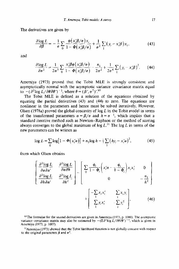
The derivatives are given by
a1og L 1 c ~(w+, --= -- ap
+kgy,-x$)x;, (J (J 14(x;&%) cJ2 1
17
(43)
and
al0gL 1 -- aa2
c x:P@ (x:&q -“I+-Qy,-x;@2. (44)
-2a3 (J 1 - @(x:/3/u) 2u2 2u4 1
Amerniya (1973) proved that the Tobit MLE is strongly consistent and asymptotically normal with the asymptotic variance-covariance matrix equal to -(a210gL/&%3P-1,where8=(p~,~2)‘.10
The Tobit MLE is defined as a solution of the equations obtained by equating the partial derivatives (43) and (44) to zero. The equations are nonlinear in the parameters and hence must be solved iteratively. However, Olsen (1978a) proved the global concavity of log L in the Tobit model in terms of the transformed parameters LY = p/u and h = u -l, which implies that a standard iterative method such as Newton-Raphson or the method of scoring always converges to the global maximum of log L.” The log L in terms of the new parameters can be written as
0
from which Olsen obtains
a2i0g L a2i0g L ___ ~ aff ad aaah
a2iog L a2iog L ___ ____ ahad ah2
_
(45)
0
n1 2 I
(46)
“The formulae for the second derivatives are given in Amemiya (1973, p. 1000). The asymptotic variance-covariance matrix may also be estimated by -(Ea210g L/~OCM’) -‘, which is given in Amemiya (1973, p. 1007).
“Amemiya (1973) showed that the Tobit likelihood function is not globally concave with respect to the original parameters B and (I’.

18 T. Amemiyq Tobir models: A SUIV~Y
where $+ = +(x+x) and Gi = @(x,%x). But, x+x - [l - @(x$)1 P1+(x$x) < 0. Therefore, the right-hand side of (46) is the sum of two negative-definite matrices and hence is negative definite.
Even though convergence is assured by global concavity, it is a good idea to start an iteration with a good estimator because it will improve the speed of convergence. Tobin (1958) used the following simple estimator based on a linear approximation of the reciprocal of Mills’ ratio to start his iteration for obtaining the MLE: By equating the right-hand side of (43) to zero, we obtain
-UC- @l x,+C(y,-x;p)x,=o. 0 I-@, 1
(47)
If we premultipIy (47) by p’/(204) and add it to the equation obtained by setting (44) equal to zero, we get
Approximate (1 - @,) -‘I#, by the linear function a + b. (x;p/o) and substitute it into the left-hand side of (47) to obtain
-uC[u+b.(x:p/u)]x,+C(y,-x:p)x,=o. 0 1
(49)
Solve (49) for p and insert it into (48) to obtain a quadratic equation in u. If the roots are imaginary, Tobin’s method does not work. If the roots are real, one of them can be chosen arbitrarily. Once an estimate of u is determined, an estimate of p can be determined linearly from (49). Amemiya (1973) showed that Tobin’s initial estimator is inconsistent. However, empirical researchers have found it to be a good starting value for iteration.
Amemiya (1973) proposed the following simple consistent estimator: We have
Combining (12) and (50) yields
E( Y,?Y, ’ 0) = x:PE(Y,IY, ’ 0) +a21 (51)
which can be alternatively written as
y;=Y,x:P+u2+5,7 for i such that y, > 0, (52)

T. Amemja, Tobit models: A survey 19
where E(&ly, > 0) = 0. Then, consistent estimates of /? and a* are obtained by applying an instrumental variables method to (52) using (GLx:, 1) as the instrumental variables where 9, is the predictor of yi obtained by regressing positive y, on x, and, perhaps, powers of xi. The asymptotic distribution of the estimator is given in Amemiya (1973). A simulation study by Wales and Woodland (1980) indicates that this estimator is rather inefficient.
4.6. The EM algorithm
The EM algorithm is a general iterative method for obtaining the MLE, first proposed by Hartley (1958) and generalized by Dempster, Laird and Rubin (1977), which is especially suited for censored regression models such as Tobit models. It has good convergence properties making it especially useful for handling the more complex Tobit models, which I will discuss later, where global concavity may not hold. However, I will discuss it in the context of the Standard Tobit model because all the essential features of the algorithm can be explained for that model. I will first present the definition and the properties of the EM algorithm under a general setting and then apply it to the Standard Tobit model.
I will explain the EM algorithm in a general model where a vector of observable variables z are related to a vector of unobservable variables y* in such a way that the value of y* uniquely determines the value of z but not vice versa. In the Tobit model, { y,*} defined in (3) constitute the elements of y*, and { y,} and { wi} defined in (4) and (9) respectively constitute the elements of z. Let the joint density or probability of y* bef( y*) and let the joint density or probability of z be g(z). Also, define k(y*)z) =f( y*)/g( z). We implicitly assume that f, g and k depend on a vector of parameters 8. The purpose is to maximize
L(e)Gn -‘logg(z) = n -ilogf(y*) -n -llogk(Y*lz), (53)
with respect to 8. Define
where we are taking expectation assuming 8, is the true parameter value, and doing this conditional on z. Then, the EM algorithm purports to maximize L(8) by maximizing Q(tYlt9,) with respect to 8 when 8, is given at each step of the iteration. The E of the name EM refers to the expectation taken in (54) and the M refers to the maximization of (54).
I will consider the convergence properties. Define
(55)

20 T. Amemiya, Tobit models: A survey
Then we have, from (53), (54), and (55) and the fact that L(810,) = L(8),
(56)
But we have by Jensen’s inequality”
(57)
Now, given 8,, let M(8,) maximize Q(el0,) with respect to 8. Then, we have
(58)
But, since Q(Mle,) 2 Q(el0,) by definition and H(Mle,) 5 H(t9#?,) by (57), we have from (56) and (58)
Thus, we have proved the desirable property that L always increases or stays constant at each step of the EM algorithm. Next, let B be the MLE. Then, L(8) 2 L[M(d)] by definition. But L(b) 5 L[ M(d)] by (59). Therefore we have
L(B)=L[M(B)], (60)
which implies that if L(8) has a unique maximum and if the EM algorithm converges, it converges to 6.
We still need to prove that the EM algorithm converges to the MLE. Unfortunately, it is never easy to find reasonable and easily verifiable condi- tions for the convergence of any iterative algorithm. Dempster et al. (1977) do not succeed in doing this. I will merely give a sufficient set of conditions below.
The conditions I impose are (A) L is bounded and (B) the smallest characteristic root of - a*Q(ele,)/aeae is bounded away from 0 for all 8, and 8. Consider
~(6) = Qwt) - mtie,), (61)
12We have by (55)
n[ ff(W’,) - WW,)] = E+%[ k(y*lWk( y*lh)] 1 where I have omitted the conditioning variable .z to simplify notation and EB, means that the expectation is taken on the assumption that the density of y* is k(y*&). But, by Jensen’s inequality [see Rao (1973, p. 149]),
E,,log[ k(y*I~).&*~Q] 6 logE8,[ W1W+*1Ql.
Thus, (57) follows from the above results and by noting
logE8,[k(y*ie)/k(Y*ie1)] =logjk(Y*le)dy* =o.

T. Amemiya, Tobit models: A suruey 21
and
W%+,) = Q(@,+,lU -W,+,l@,). (62)
Since we previously established L( 0,+ i) 1 L( 0,) assumption (A) implies lim r_ ,[ L( 0,+ i) - L(e,)] = 0. Therefore, from (61) and (62) and using (57) and Q(e,+,]e,) 2 (e,]&) by definition we have
hm [Q(e,+,]e,) - eovt~l = 0. (63) T’cc
Now, denoting only the first argument of Q and suppressing its second argument, we have by a Taylor expansion of Q(k),) about Q(8,+i)
e(e,+l>-e(e,>=~(e,-e,+,>‘[-a*p/aeae~l(e,-e,+,) 2- 9, a - t+I)‘(e - er+dy (64)
where the matrix of the second derivatives is evaluated at a point between 0,
and q+i and h, denotes its smallest characteristic root. Note that in obtaining the equality above I have noted aQ(0,+,l0,)/@+, = 0 by definition. Thus, (63) (64) and assumption (B) imply
lim (er+l - e,) = 0, (65) r-+m
meaning that the EM algorithm converges.13
Now, consider an application of the algorithm to the Tobit model.14 Define 8 = (/3’, a’)‘. Then, in the Tobit model we have
iogf(y*le) = - ti0g a2 - -$ ,gl (y,* - x:P)21 (66)
and, for a given estimate 0i = (pi, a:)‘, the EM algorithm maximizes with respect to p and u*
E[logf(Y*i0Y,w, 41 = - ;1ogo* -shiv,-x:P)‘-~~E[(y:-x:P):ly=O,e,]
1 0
= - ;1ogo* -~~(Y;-~;B)*-~~[“(Y~lw,=o.8’)-x;~]~
(67)
“See Wu (1983) for more discussion of the convergence of the EM algorithm
14For an alternative account, see Hartley (1976~).

22 T. Amemiya, Tobit models: A sumey
where
and
v( y,*lw, = 034) = 0: + x:&[v#d(l - @,>I - b1w0 - WI*,
(69)
where $r = $(x,!/3r/ui) and @r = @(~~&/a~).
From (67) it is clear that the second-round estimate of p in the EM algorithm, denoted &, is obtained as follows: Assume without loss of general- ity that the first n, observations of Y, are positive and call the vector of those observations Y as I did in (20). Next, define an (n - n,)-vector Y* whose elements are the Y,’ defined in (68). Then, we have
p*= (xx-‘X’ ;. , [ 1
(70)
where X was defined after (4). In other words, the EM algorithm amounts to predicting all the unobservable values of Y,* by their conditional expectations and treating the predicted values as if they were the observed values. The second-round estimate of u2, denoted a;, is given by
(72 2=n-’
~(Y,-X:P2)2+~(Y~-Xl~2)2+~~(Y~l~,=O~~I) . 1 (71)
Although this follows from the general theory of the algorithm given earlier, we can also directly show that the MLE 4 is the equilibrium solution of the iteration defined by (70) and (71). Partition X = (X’, X0’)’ so that X is multiplied by y and X0 by y”. Then, inserting 6 into both sides of (70) yields, after collecting terms,
x@ = xly - x0/[ b#J( x$/&)/(1 - @(x$/G))] ) (72)
where the last bracket denotes an (n - n,)-dimensional vector whose typical element is given inside. But, clearly, (72) is equivalent to (47). Similarly, the MLE 4 can be shown to be an equilibrium solution of (71).
Unfortunately, conditions (A) and (B) do not generally hold for the Tobit model. However, they do hold if the sample size is sufficiently large and if the iteration is started from a point sufficiently close to the MLE. Schmee and

T. Amemiya, Tobit models: A sutv~v 23
Hahn (1979) performed a simulation study of the EM algorithm applied to a censored regression model (a survival model) defined by
Y, = Y, if y,*sc,
=C if y;*>c,
where y,* - N(cu + /3x,, a*). They generally obtained rapid convergence.
5. Properties of the Tobit MLE under non-standard assumptions
In this section I will discuss the properties of the Tobit MLE - the estimator which maximizes (42) - under various types of non-standard assumptions: heteroscedasticity, serial correlation, and non-normality. It will be shown that the Tobit MLE remains consistent under serial correlation but not under heteroscedasticity or non-normality. The same is true of the other estimators considered earlier. This result contrasts with the classical regression model in which the least squares estimator (the MLE under the normality assumption) is generally consistent under all of the three types of non-standard assumptions mentioned above.
Before proceeding with rigorous argument, I will given an intuitive explana- tion of the above-mentioned result. By considering (17) we see that serial correlation of y, should not affect the consistency of the NLLS estimator, whereas heteroscedasticity changes (I to a, and hence invalidates the estimation of the equation by least squares. If y,* is not normal, eq. (17) itself is generally invalid, which leads to the inconsistency of the NLLS estimator. Though the NLLS estimator is different from the ML estimator, one can expect a certain correspondence between the consistency properties of the two estimators.
5.1. Heteroscedasticity
Hurd (1979) evaluated the probability limit of the truncated Tobit MLE when a certain type of heteroscedasticity is present in two simple truncated Tobit models: (1) the i.i.d. case (that is, the case of the regressor consisting only of a constant term) and (2) the case of a constant term plus one independent variable. Recall that the truncated Tobit model is the one in which no information is available for those observations for which y,* < 0 and therefore the MLE maximizes (6) rather than (5).
In the i.i.d. case, Hurd created heteroscedasticity by generating rn observa- tions from N(p, u,‘) and (1 - r)n observations from N(p, u,‘). In each case, he recorded only positive observations. Let y,, i = 1,2,. . . , n,, be the recorded observations. (Note n, 2 n.) One can show that the truncated Tobit MLE of p and (I *, denoted p and h2, are defined by equating the first two population

24 T. Amemiya, Tobit models: A survey
moments of y, to their respective sample moments,
(73) i=l
and
8*+8PX(~/6)+82=n,l~~~. (74) r=l
Taking the probability limit of both sides of (73) and (74) and expressing plim n;‘C_yi and plim “1 ‘c ? yl as certain functions of the parameters ~1, a:, q? and r, one can define plim fi and plim8* implicitly as functions of these parameters. Hurd evaluated the probability limits for various values of p and ui after having fixed r = 0.5 and a2 = 1. Hurd found large asymptotic biases in certain cases.
In the case of one independent variable, Hurd generated observations from N( (Y + /3x,, u,‘) after having generated xi and loglu,\ from Bivariate N(O,O, VP, I’:, p). For given values of (Y, p, Vi, V, and p, Hurd found the values of LX, p and u* that maximize Elog L, where L is as given in (6). Those values are the probability limits of the MLE of (Y, j3 and u2 under Hurd’s model if the expectation of log L is taken using the same model. Again, Hurd found extremely large asymptotic biases in certain cases.
Arabmazar and Schmidt (1981) show that the asymptotic biases of the censored Tobit MLE in the i.i.d. case are not as large as those obtained by Hurd.
5.2. Serial correlation
Robinson (1982a) proved the strong consistency and the asymptotic normal- ity of the Tobit MLE under very general assumptions about U, (normality is presupposed) and obtained its asymptotic variance-covariance matrix, which is complicated and therefore not reproduced here. His assumptions are slightly stronger than the stationarity assumptions but are weaker than the assumption that U, possesses a continuous spectral density. His results are especially useful since the full MLE that takes account of even a simple type of serial correlation seems computationally intractable. The autocorrelations of U, need not be estimated in order to compute the Tobit MLE but must be estimated in order to estimate its asymptotic variance-covariance matrix. The consistent estimator proposed by Robinson (1982b) may be used for that purpose.
5.3. Non-normality
Goldberger (1980) considered an i.i.d. truncated sample model in which data are generated by a certain non-normal distribution with mean p and variance 1 and are recorded only when the value is smaller than a constant c. Let y

T Amemiyo, Tobit models: A sumq 25
represent the recorded random variable and let 7 be the sample mean. The researcher is to estimate p by the MLE assuming that the data are generated by N(p, 1). As in Hurd’s i.i.d. mode!, the MLE fi is defined by equating the population mean of y to its sample mean,
/i-qc-fi)=y. (75)
Taking the probability limit of both sides of (75) under the true model and putting plim ji = p* yields
p*-X(c-p*)=p-h(c-P)? (76)
where h( c - I*) = E(I_~ - yl y -C c), the expectation being taken using the true model. Defining m = p* - p and 8 = c - p, we rewrite (76) as
m=A(e-m)-h(e). (77)
Goldberger calculated M as a function of B when the data are generated by Student’s t with various degrees of freedom, Laplace and logistic distributions. The asymptotic bias was found to be especially great when the true distribu- tion is Laplace. Goldberger also extended the analysis to the regression model with a constant term and one discrete independent variable. Arabmazar and Schmidt (1982) extended Goldberg’s analysis to the case of an unknown variance and found that the asymptotic bias was further accentuated.
5.4. Tests for normality
The fact that the Tobit MLE is generally inconsistent when the true distribution is non-normal makes it important for a researcher to test whether his data are generated by a normal distribution. Nelson (1981) devised tests for normality in the i.i.d. censored sample model and the Tobit model. His tests are applications of the specification test of Hausman (1978).
In Hausman’s test, one uses the MLE B obtained under the null hypothesis, which is asymptotically efficient under the null hypothesis but loses consistency under an alternative hypothesis, and a consistent estimator 8, which is asymp- totically less efficient than the MLE under the null hypothesis but remains consistent under an alternative hypothesis. Hausman (1978) noted that (4 - (?)‘V-‘(f? - 8) is asymptotically distributed under the null hypothesis as &i-square with K degrees of freedom (K being the number of elements in 8) where V= I’(e) - V(g), the difference of the asymptotic variance-covariance matrices evaluated under the null hypothesis. An advantage of Hausman’s test is that one need not know the covariance between fi and 4 to perform the test.

26 T. Amemiya. Tobit models: A survey
Nelson’s i.i.d. censored sample model is defined by
Y, = Y, if y;*>O,
= 0 if y,* 5 0, i=1,2 ,..., n,
where y,* - N( ~1, a2) under the null hypothesis. Nelson considers the estima- tion of P( y,* > 0). Its MLE is #(P/I?) where r_i and 6 are the MLE of the respective parameters. A consistent estimator is provided by n/n where, as before, n, is the number of positive observations of y,. Clearly, nl/n is a consistent estimator of P( y,* > 0) under any distribution provided that it is i.i.d. Nelson derived the asymptotic variances under normality of the two estimators.
If we interpret what one is estimating by the two estimators as lim,,,n -‘Z;= iP( y,* > 0), Nelson’s test can be interpreted as a test of the null hypothesis against a more general misspecification than just non-normal- ity. In fact, Nelson conducted a simulation study to evaluate the power of the test against a heteroscedastic alternative. The performance of the test was satisfactory but not especially encouraging.
In the Tobit model, Nelson considers the estimation of
Its MLE is given by the right-hand side of this equation evaluated at the Tobit MLE, and its consistent estimator is provided by n -‘X’y. Hausman’s test based on these two estimators will work because this consistent estimator is consistent under general distributional assumptions on y. Nelson derived the asymptotic variance-covariance matrices of the two estimators.
Nelson was ingenious in that he considered certain functions of the original parameters for which one can easily obtain estimators which are consistent under very general assumptions. However, it would be better if one could find a general consistent estimator for the original parameters themselves. An example is Powell’s least absolute deviations estimator, which I discuss below.
Bera, Jarque and Lee (1982) propose using Rao’s score test in testing for normality in the standard Tobit model where the error term follows the two-parameter Pearson family of distributions, which contains normal as a special case.
5.5. Non-normal Tobit
If ui in the Tobit model (3) is not normal, one of two things can be done: (1) Specify a non-normal distribution and use the true MLE or some other estimator tailor-made for the distribution. (2) Use an estimator which is consistent under general distributions, both normal and non-normal. In this
T Amemiya, Tobif models: A survey 27
subsection I give examples of the first approach. An example of the second approach is given in the next subsection.
Amemiya and Boskin (1974) studied the effect of wage and other indepen- dent variables on the number of months during a five-year period in which a household received welfare payments. Since the dependent variable is naturally bounded between 0 and 60, one must impose both an upper and lower truncation point if one uses a normal Tobit model. Instead, the authors assumed the dependent variable to be lognormal and hence positive, so that only an upper truncation needs to be imposed. The MLE was used.
Pokier (1978) considers the model in which the dependent variable y is constrained by a <_y < b and its Box-Cox transformation (y’ - 1)/h is trun- cated normal.
The majority of models I will discuss in part II assume a normal distribu- tion. Exceptions are some of the models proposed by Cragg (1971) mentioned in footnote 15 and the model of Dubin and McFadden (1980) discussed in section 11.7.
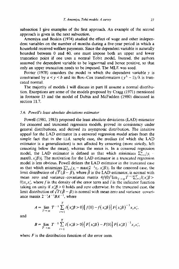
5.6. Powell’s least absolute deviations estimator
Powell (1981, 1983) proposed the least absolute deviations (LAD) estimator for censored and truncated regression models, proved its consistency under general distributions, and derived its asymptotic distribution. The intuitive appeal for the LAD estimator in a censored regression model arises from the simple fact that in the i.i.d. sample case, the median (of which the LAD estimator is a generalization) is not affected by censoring (more strictly, left censoring below the mean), whereas the mean is. In a censored regression model, the LAD estimator is defined as that which minimizes C:=,Jy, - max(O, x,‘p)I. The motivation for the LAD estimator in a truncated regression model is less obvious. Powell defines the LAD estimator in the truncated case as that which minimizes C:=,l_y, - max(2-‘y,, x:/3)/. In the censored case, the limit distribution of 0(/I - p), where b is the LAD estimator, is normal with mean zero and variance-covariance matrix 4f(O)*limr, ,,T -‘,I~= II( x;p > 0)x,x:, where f is the density of the error term and 1 is the indicator function taking on unity if xi/3 > 0 holds and zero otherwise. In the truncated case, the limit distribution of @(B - /?) . IS normal with mean zero and variance-covari- ante matrix 2 - ‘A _ ‘BA _ ‘, where
A = Fimrn +(x:8 > O)[f(O) -f(x$)] F(x:P)-lx,x:. and
B=+>aT’ i I(~;P~O)[F(X;~)-F(O)]F(X;~)-~X,~;, t=1
where F is the distribution function of the error term.

28 T. Amemiya, Tobit models: A survey
Powell’s estimator is attractive because it is the only known estimator which is consistent under general non-normal distributions. However, its main drawback is the computational difficulty it entails. Paarsch (1984) conducted a Monte Carlo study to compare Powell’s estimator, the Tobit MLE, and Heckman’s two-step estimator in the standard Tobit model with one exogenous variable under situations where the error term is distributed as normal, exponential and Cauchy. Paarsch found that when the sample size is small (50) and there is much censoring (50% of the sample), the minimum frequently occurred at the boundary of a wide region over which a grid search was performed. In large samples Powell’s estimator appears to perform much better than Heckman’s estimator under any of the three distributional assumptions and much better than the Tobit MLE when the errors are Cauchy.
Another problem with Powell’s estimator is finding a good estimator of the asymptotic variance-covariance matrix, which does not require the knowledge of the true distribution of the error. Powell (1983) proposes a consistent estimator.
Poweli observes that his proof of the consistency and asymptotic normality of the LAD estimator generally holds even if the errors are heteroscedastic. This fact makes Powell’s estimator further attractive because the usual estima- tors are inconsistent under heteroscedastic errors as noted earlier.
6. Variations of the Standard Tobit model
In this section I discuss a few models that are variations on the Tobit model. More significant generalization of the Tobit model are discussed in part II.
Rosett (1959) proposed a model in which the observable random variables { y, } are defined by
Y; = Y? if yi*sO,
= 0 if O<y,* <c~, (78)
=yT-a if (Y 4 yi*, i= 1,2 ,..., n,
where y,* - N(x(& a2). One can estimate a as well as /I and u2. Rosett called it a model of friction because the model implies that the dependent variable assumes a certain value (in this case 0) until a change in an independent variable overcomes the friction. At this point the dependent variable either increases or decreases depending upon the type of the stimulus. Maddala (1977) remarks that this model is useful in analyzing dividend policies, changes in wage offers by firms, and similar examples where firms respond by jumps after a certain cumulative effort.

T. Amemiya, Tobit models: A survey 29
Rosett and Nelson (1975) considered the following simple generalization of the Tobit model:
Y, = a1 if y,* 5 al,
= Y, if al <yT < az, (79)
=a 2 if a2Ql*,
where y,* - N(x(/3, a2). If xi contains a constant term, one can assume a1 = 0 without loss of generality. Then, the Standard Tobit model is obtained as a special case by putting a2 = w. According to Maddala (1977a), an example of a problem to which this model has been applied is the demand for health insurance by people on medicare, where both a minimum coverage and a maximum amount are imposed.
Dagenais (1969) proposed a model which is obtained by making the boundary points of Rosett’s model stochastic as follows:
Y, =y,* if Yi* 5 Ui,
= 0 if ui < yi* < xiy + W,, (80)
= y,* - x,fy if X,!y + Wi 5 yj*,
where yi* - N(x$, a2) and u, and w, are also normal. Unfortunately, there is a logical inconsistency in the model because ui -C x,‘y + w, cannot always be guaranteed. Perhaps for this reason, this model does not seem to have been applied to real data. Dagenais (1975) begins to discuss this model but the model he actually estimated is of Type 2 Tobit, which I will discuss later.
II. Generalized Tobit Models
7. Introduction
As I stated in section 1, I will classify the majority of Tobit models into five common types according to similarities in the likelihood function. Type 1 is the Standard Tobit model which I have discussed in part I. In part II, I will define and discuss the remaining four types of Tobit models.
It is useful to characterize the likelihood function of each type of model schematically as in table 1, where each Y,, i = 1,2,3, is assumed to be distrib- uted as N(x,$,, uj2), and P denotes a probability or a density or a combination thereof. One is to take the product of each P over the observations that belong to a particular category determined by the sign of y,. Thus, in Type 1

30 T. Amemiya, Tobit models: A survey
Table 1
Type 1 P(Y, < O).fvYl) 2 P(y, < 0). QYI ’ 0, Y2)
3 P(Y, <O)‘P(Y,*Y2) 4 P(Y,<O*Y,)~P(Y,1Y2) 5 P(y, < 0, Y,)‘P(Y, ’ 0, Y2)
(Standard Tobit model), P(y, < 0). P(yl) is an abbreviated notation for n,P( y: < 0) .n,fii( _yi,), wherefn is the density of N( xi,&, u-i?). This expres- sion can be rewritten as (5) after dropping the unnecessary subscript 1.
Another way to characterize the five types is by the classification of the three dependent variables which appear in table 2. In table 2 below, B is an abbreviation for Binary and C for Censored. In each type of model, the sign of y, determines one of the two possible categories for the observations, and a censored variable is observed in one category and unobserved in the other. Note that when y, is labelled C, it plays two roles: the role of the variable whose sign determines categories and the role of a censored variable.
We allow for the possibility that there are constraints among the parameters of the model (/I,, u,~), i = 1,2,3. For example, constraints will occur if the original model is specified as a simultaneous equations model in terms of y,, y, and y,. Then, the p’s denote the reduced-form parameters.
I will not discuss here models in which there are more than one binary variable and, hence, models whose likelihood function consists of more than two components. Such models are computationally more burdensome because they involve double or higher-order integration of joint normal densities. The only exception occurs in section 11.7, which includes models that are obvious generalizations of the Type 5 Tobit model. Neither will I discuss a simulta- neous-equation Tobit model of Amemiya (1974b). The simplest two-equation case of this model is defined by y,, = max(y,Y2, + xi,& f ui,,O) and y,, = max(y,y,, + x&f12 + u~~,O) where (uli, u2,) is bivariate normal and yly2 < 1 must be assumed for the model to be logically consistent. A schematic representation of the likelihood function of this two equation model is
KY,, y2). KY, < 0, y3). W2 < 0, IQ. f’03 < 0, .Y, < 0) with Y’S w- propriately defined.
Table 2
Yl Y2 Y3
Type 1 c 2 B C 3 c C 4 C C C 5 B C C

T. Amemiya, Tobit models: A survey 31
8. Type2:P(y,<o)*~(Yt’“,yZ)
8.1. Definition and estimation
The Type 2 Tobit model is defined as follows:
Y2r = v2: if y: > 0, (81)
= 0 if yc 5 0, i=1,2 n, ,...,
where {q,, u2r} are i.i.d. drawings from a bivariate normal distribution with mean zero, variances I$ and a:, and covariance q2. It is assumed that only the sign of yz is observed and that yz is observed only when yc > 0. It is assumed that xi, are observed for all i but x2i need not be observed for i such that yc 5 0. One may also define, as in (9).
wi, = 1 if yc > 0,
=0 if ~650. (82)
Then, { wir, y2, } constitute the observed sample of the model. It should be noted that, unlike the Type 1 Tobit, y,, may take negative values.15 As in (4), y2, = 0 merely signifies the event y{ =< 0.
The likelihood function of the model is given by
~=~P(Y;:40)~~(y,,lYl:>O)P(Y,:>o), (83)
where n, and n, stand for the product over those i for which y,, = 0 and y2, # 0, respectively, and f( .Iyc > 0) stands for the conditional density of yz given yc > 0. Note the similarity between (7) and (83). As in Type 1 Tobit, one can obtain a consistent estimate of &/a, by maximizing the probit part of
(83)
ProbitL=yP(y$jO)vP(yl:>O). (84)
Also, (84) is a part of the likelihood function for every one of the five types of models; therefore, a consistent estimate of &/a, can be obtained by the probit MLE in each of these types of model.
“See Cragg (1971) for models which insure the non-negativity of yz as well as _yl.

32 T. Amemiya, Tobit models: A suruey
One can rewrite (83) as
(85)
where f( ., .) denotes the joint density of y: and ~2.. One can write the joint density as the product of a conditional density and a marginal density, i.e.,
f(y& ~~~1 =.f(yl:I~~~).f(y~,), and deterfine a specific form forf(yCl~~,) from the well-known fact that the conditional distribution of yc given yz = y2, is normal with mean xl,& + o12u2- *(yZi - x&fi2) and variance u: - u&u2- *. Thus, one can further rewrite (8.5) as
X~@([x;i~lu<l+u u-'"~2(Y2i-x~~P2)] 12 1
x [ 1 - uf2u1- Zu2- * ]~‘)“~‘~[u;1(Y2~-x;ia)]’ (86)
Note that L depends on ur only through &ul~’ and u12ulP1; therefore, if there is no constraint on the parameters, one can put o1 = 1 without any loss of generality. Then, the remaining parameters can be identified. If, however, there is at least one common element in & and P2, u1 can be also identified.
I will show how Heckman’s two-step estimator can be used in this model. To obtain an equation comparable to (17), we need to evaluate E( yz]y;: > 0). For this purpose we use the well-known result
where c2, is normally distributed independently of yl”; with mean zero and variance u; - ~~~a;‘. Using (87), one can express E( $1~1: > 0) as a simple linear function of E(y,:ly;: > 0), which was already obtained in part I. Using (87), one can also derive V( y; Iyc > 0) easily. Thus, we obtain
y,, = x;,b2 + u,,u<‘h( ~;,a,) + &2i, for i such that ~2, > 0, (88)
where CX~ = &cJ-~, EeZi = 0, and
VEZi = Cl; - u~2ul- = [ XL”lh(x~ial) +x(xLal)2]. (89)
As in the case of the Type 1 Tobit, Heckman’s two-step estimator is the LS estimator applied to (88) after replacing (Y~ with the probit MLE. The asymp-

T. Amemiya, Tobit models: A survey 33
totic distribution of the estimator can be similarly obtained as in section 4.3 by defining Q; in the same way as before. It was first derived by Heckman (1979).
The Standard Tobit (Type 1) is a special case of Type 2, in which y$ = ~2:. Therefore, (88) and (89) will be reduced to (17) and (18) by putting xl,& = xi,& and a*=a:=a .
A g&teralizati& of the two-step method applied to (29) can be easily defined for this model but will not be discussed.
It is important to note, as pointed out by Olsen (1980) that the consistency of Heckman’s estimator does not require the joint normality of y: and y$ provided that y: is normal and eq. (87) holds with l2 independently distributed of y: but not necessarily normal. For, then, (88) would be still valid. As pointed out by Lee (1982) the asymptotic variance-covariance matrix of Heckman’s estimator can be consistently estimated under these less restrictive assumptions by using White’s estimator analogous to the one mentioned after eq. (28). Note that White’s estimator does not require (89) to be valid.
8.2. A special case of independence
Dudley and Montmarquette (1976) analyzed whether or not the United States gives foreign aid to a particular country and, if it does, how much foreign aid it gives using a special case of the model (81) where the indepen- dence of ul, and u2, is assumed. In their model, the sign of yz determines whether aid is given to the i th country, and y$ determines the actual amount of aid. They used the probit MLE to estimate /$ (assuming u1 = 1) and the least squares regression of y,, on x*1 to estimate &. The LS estimator of & is consistent in their model because of the assumed independence between uli and uZI_ This makes their model computationally advantageous. However, it seems unrealistic to assume that the potential amount of aid. y;, is indepen- dent of the variable which determines whether or not aid is given, y;“. This model is the opposite extreme of the Tobit model, which can be regarded as a special case of Type 2 model where there is total dependence between y: and yz, in the whole spectrum of models (with varying correlation between y;* and y;) contained in Type 2.
Because of the computational advantage mentioned above, this ‘indepen- dence’ model and its variations were frequently used in econometric applica- tions in the 1960’s and early 70’s. In many of these studies, authors made the additional linear probability assumption: P(y;l > 0) = xii&, which enabled them to estimate & (as well as /3,) consistently by the least squares method. For examples of these studies, see Huang (1964) and Wu (1965).
8.3. Gronau (1973)
I take up Gronau’s model as the first example of the Type 2 Tobit model because he seems to be the first person to suggest an empirical model of this

34 T. Amemiya, Tobit models: A survey
type, even though he did not use all the information provided by the model and sometimes used incorrect estimation procedures, as I will show below. His model of labor supply, based on the idea of a reservation wage, has since been used and extended by many authors.
First, I will briefly sketch Gronau’s theory of how a housewife decides whether or not to work and how much to work. Gronau assumes that the offered wage IV0 is given to each housewife independently of hours worked H, rather than as a schedule W’(H). Given IV’, a housewife maximizes her utility function U(C, X) subject to X = W”H + V and C + H = T, where C is time spent at home for child care, X represents all other goods, T is total available time, and V is other income. Thus, a housewife does not work if
and works if the inequality in (90) is reversed. If she works, the hours of work H and the actual wage rate W must be such that
(au/ac)/( au/ax) = w.
Gronau calls the left-hand side of (90) the housewife’s value of time, or, more commonly, the reservation wage, denoted W’.16
Assuming that both W” and W’ can be written as linear combinations of independent variables plus error terms, his model may be statistically de- scribed as follows:
w” = x;ip* + U2*, wr = z,!a + ui,
w,=H$O if I?$‘> yr, (91)
= 0 if W;Os Kr, i=1,2 n, ,**-,
where (u,~, u,) is an i.i.d. drawing from a bivariate normal distribution with mean zero, variances u,’ and u,‘, and covariance uUU. Thus, the model can be written in the form of (81) by putting y” - wr =yc and y” = y& Note that H (hours worked) is not explained by this statistical model though it is determined by Gronau’s theoretical model. A statistical model explaining H as well as W was later developed by Heckman (1974). I will discuss this in the section on Type 3 models.
Since the model (91) can be transformed into the form (81) in such a way that the parameters of (91) can be determined from the parameters of (Sl), all
16For a more elaborate derivation of the reservation wage model based on search theory, see Gronau (1974).

T. Amemiya, Tobit models: A survey 35
the parameters of the model are identifiable except V( FI$’ - I+$‘), which can be set equal to 1 without loss of generality. If, however, at least one element of xZi is not included in zi, all the parameters are identifiable.17 They can be estimated by the MLE or Heckman’s two-step estimator by procedures de- scribed in section 8.1 above. One can also use the probit MLE (the first step of Heckman’s two-step) to estimate a certain subset of the parameters. However, the main estimation method used by Gronau is not among the above. I will describe his method after correcting a minor error.
The full likelihood function of Gronau’s model (91) can be written as
(92)
where no and n, are the products over those observations for which w:” 5 y’ and w” > er, respectively, and f(. , -) is the joint density of u/;’ and w:‘. Gronau assumes that u2, and u, are independent.18 Under this assumption, (92) can be written as
where
Maximizing (93) yields the MLE of (Y, &, a,, and au, which are consistent and asymptotically efficient under Gronau’s independence assumption. Maximizing (94) yields estimates of (Y, & and a0 which are consistent but asymptotically not fully efficient.
Gronau’s method consists of two steps. The first step is carried out as follows: We have under Gronau’s independence assumption
E(qJ&‘< ~“)=x;i&+(~~+u~)-tu~@i-l~;r (95)
“Gronau specifies that the independent variables in the W’ equation include woman’s age and education, family income, number of children, and husband’s age and education, whereas the independent variables in the W” equation include only woman’s age and education. However, Gronau readily admits to the arbitrariness of the specification and the possibility that ah the variables are included in both.
‘sThis may not be a realistic assumption since common independent variables, which are excluded from the set of regressors, may be included in both u, and u,. The assumption is not necessary if one uses either the MLE or Heckman’s twostep estimator. It should be noted that the independence of u, and u, does not imply the independence of ut, and us, in (81) so that Gronau’s model is not as simple as the model considered in section 8.2 above. Also note that this assumption makes all the parameters identifiable even if no element of a is set equal to zero.

36 T. A memiya, Tobir models: A survey
where +, and Qi are + and @ evaluated at (u,’ + u,‘) -f(xGifi2 - ~;a). Since Gronau’s data are such that there are many individuals with the same value of the independent variables, one can estimate Gi directly by the ratio of the number of working wives to the number of wives with the characteristics xi. Given this estimate, denoted &;, one can estimate & by 6; = cp[ Cp -‘( !&;)I. Next, one regresses positive w on x2i and &i:.-lq$ to estimate p2. This estimate, denoted fi2, is consistent (provided that the above estimates of 9; and !P, are consistent), and, therefore, the first problem of the first estimation method is solved. In the second step, Gronau maximizes L* after replacing /3* by &.”
Despite the minor error in the estimation method, Gronau’s article made a significant econometric contribution (besides a substantive empirical contribu- tion which I have ignored) by suggesting a two-step method based on the conditional expectation equation, which became a precursor of Heckman’s two-step estimator.
8.4. Other applications
Nelson (1977) noted that a Type 2 Tobit model arises if y,, in (1) is assumed to be a random variable with its mean equal to a linear combination of independent variables. He reestimated Gronau’s model by maximizing the correct likelihood function (93).
Dagenais (1975) used a Type 2 Tobit model to analyze household purchase of automobiles. In this model, y; in (81) represents the desired expenditure on a car and x2 includes permanent income, education, and the number of children. He assumes that a household purchases a car if yc exceeds a stochastic threshold S = 8, + 0,,4 + u, where A is the dummy variable taking unity if the household anticipated buying a car at the time of a prior questionaire and the actual value of purchase y, =yT if v? > S. Thus, _Y; - S plays the role of JJ: in (81). Like Gronau, Dagenais assumes independence between y? and S, and, in addition, he assumes equality of the variances of y? and S. These assumptions are not necessary for identification. Dagenais’ model, like Gronau’s, has a weakness in that an arbitrary separation of the independent variables into some which go into the _@ equation and some which go into the S equation (IV’ equation and IV0 equation in Gronau’s model) is maintained.
In the study of Westin and Gillen (1978), u; represents the parking cost with x2 including zonal dummies, wage rate (as a proxy for value of walking time), and the square of wage rate. A researcher observes ~2 = y, if y? < C where C represents transit cost, which itself is a function of independent variables plus an error term.
19Gronau actually omitted 0, from the expression for L*, which renders his estimates incon- sistent.

T. Amemiya, Tobit models: A sutvq 31
9. Type3 P(y,<O)*P(y,,Yz)
9.1. Definition and estimation
The Type 3 Tobit model is defined as follows:
Yli = Vii if y$ >O, (96)
Y2, = r2: if yz>O,
= 0 if j$~O, i=1,2 n, ,...,
where {or,, uzi} are i.i.d. drawings from a bivariate normal distribution with mean zero, variances uf and u;, and covariance ur2. Note that this model differs from Type 2 only in that y; is also observed when it is positive in this model.
Since the estimation of this model can be handled similarly to that of Type 2, I will discuss it only briefly. Instead, in the following I will give a detailed discussion of the estimation of Heckman’s model (1974), which constitutes the structural-equations version of the model (96).
The likelihood function of the model (96) can be written as
wheref( ., .) is the joint density of _~fi and J$ Since _~l’; is observed when it is positive, all the parameters of the model are identifiable, including uf.
Heckman’s two-step estimator was originally proposed by Heckman (1976a) for this model. Here we obtain two conditional-expectation equations, eqs. (17) and (88), for yi and y2, respectively. [Add subscript 1 to all the variables and the parameters in (17) to conform to the notation of the present section.] In the first step of the method, ai = &a~’ is estimated by the probit MLE &i. In the second step, least squares is applied separately to (17) and (88) after replacing a, by hr. The asymptotic variance-covariance matrix of the resulting estimates of (pi, al) is given in (28) and that for (p,, ulzul-‘) can be similarly obtained. The latter is given by Heckman (1979). A consistent estimate of a2 can be obtained using the residuals of eq. (88). As Heckman (1976a) suggested and as I noted in section 4.3, a more efficient WLS can be used for each equation in

38 T. Amemiya, Tobir models: A survty
the second-step of the method. An even more efficient GLS can be applied simultaneously to the two equations. However, even GLS is not fully efficient compared to MLE, and the added computational burden may not be suffi- ciently compensated for by the gain in efficiency. A two-step method based on unconditional means of y, and y2, which is a generalization of the method discussed in section 3.3, can be also used for this model.
Wales and Woodland (1980) compared the LS estimator, Heckman’s two-step estimator, probit MLE, conditional MLE (using only those who worked), MLE, and another inconsistent estimator in a Type 3 Tobit model in a simulation study with one replication (sample size 1000 and 5000). The particular model they used is the labor supply model of Heckman (1974), which I will discuss in the next subsection. ” the LS estimator was found to be poor, and all three ML estimators were found to perform well. Heckman’s two-step estimator was ranked somewhere between LS and MLE.
9.2. Heckman (1974)
Heckman’s model differs from Gronau’s model (91) in that Heckman includes the determination of hours worked H in his model.*’ Like Gronau, Heckman assumes that the offered wage IV0 is given independently of H; therefore, Heckman’s W” equation is the same as Gronau’s:
q” = x&/3* + u2i. (98)
Heckman defines W’ = (&Y/aC)/( SJ/dX) and specifies22
qr=yHi+z;ct+vi. (99)
It is assumed that the ith individual works if
~r(Hi=O)=t(a+vi< w”, (100)
and then, the wage q and hours worked Hi are determined by solving (98) and (99) simultaneously after putting W;.‘= W;:l= w. Thus, we can define
“Though Heckman’s model (1974) is a simultaneous-equations model, Heckman’s two-step estimator studied by Wales and Woodland is essentially a reduced-form estimator which I have discussed in the present section, rather than the structural equation version I will discuss in the next subsection.
“For a panel-data generalization of Heckman’s model, see Heckman and MaCurdy (1980).
22Actually, Heckman uses log W’ and log W”. The independent variables x2 include husband’s wage, asset income, prices, and individual characteristics, and the z include housewife’s schooling and experience.

T. Amemiya, Tobit models; A sutvey 39
Heckman’s model as
6 = x;,p* + U2;r (101) and
W=yyHi+z,~CY+ui, (102)
for those i for which desired hours of work
H,* = x;,pl + u1; > 0, (103)
where x;J?r = y-‘(x$,p2 - z(a) and pi, = y P1(~2i - u;). Note that (100) and (103) are equivalent because y > 0.
I will call (101) and (102) the structural equations; then, (101) and the identity part of (103) constitute the reduced form equations. The reduced form equations of Heckman’s model can be shown to correspond to the Type 3 Tobit model (96) if we put H* =yT, H=y,, W”=y,“, and W=y,. Since I have already discussed the estimation of the reduced-form parameters in the context of the model (96), I will now discuss the estimation of the structural parameters.
Heckman (1974) estimated the structural parameters by MLE. In the next two subsections I will discuss three alternative methods of estimating the structural parameters.
9.3. Heckman (I 976a)
This articles proposes the Heckman two-step estimator of the reduced-form parameters, which I have discussed in section 9.1 above, but also reestimates the labor supply model of Heckman (1974) using the structural equation version. Since (101) is a reduced-form as well as a structural equation, the estimation of p2 is done in the same way as I have discussed in section 9.1: namely, by applying least squares to the regression equation for E( W 1 Hi* > 0) after estimating the argument of A (the hazard rate) by probit MLE. So I will only discuss the estimation of (102) here. Rewrite (102) as
H,=y-‘~-~;ay-~-y-~o,. 004)
By subtracting E(qlH,* P 0) from ui and adding the same, we rewrite (104) further as
H,=y-‘~-z,‘cry-‘-al,o,‘y-‘h(x;i&/al)-y-l~i, (105)
where ulU = cov(+, ui), u; = Vuli and E; = u, - E( u, 1 Hi* > 0). Then, consistent

40 T. Amemiya, Tobit models: A sumey
estimates of y-l, (my-’ and (~i~ui-~y-~ are obtained by the least squares regression applied to (105) after replacing &/a, by its probit MLE and y by lI$, the least squares predictor of W, obtained by applying Heckman’s two-step estimator to (101). The asymptotic variance-covariance matrix of this estima- tor can be deduced from the results in Heckman (1978) who considered the estimation of a more general model (which I will discuss in the section on Type 5 Tobit models).
Actually, there is no apparent reason why one must first solve (102) for H, and proceed as I have indicated above. Heckman could just as easily have subtracted and added EZ(o,lH,* > 0) to (102) itself and proceeded similarly. This method would yield alternative consistent estimates. Inferring from a well-known fact that the two-stage least squares estimates of the standard simultaneous equations model yield asymptotically equivalent estimates re- gardless of which normalization is chosen, I conjecture that the Heckman two-step method applied to (102) and (104) would also yield asymptotically equivalent estimates of y and a.
Lee, Maddala and Trost (1980) extended Heckman’s simultaneous-equations two-step estimator and its WLS version (taking account of the heteroscedastic- ity) to more general simultaneous-equations Tobit models and obtained their asymptotic variance-covariance matrices.
9.4. Amemiya’s LS and GLS
Amemiya (1978 and 1979) proposed a general method of obtaining the estimates of the structural parameters from given reduced-form parameter estimates in general Tobit-type models and derived the asymptotic distri- bution. Suppose that a structural equation and the corresponding reduced-form equations are given by
y= Yy+X#+u, [y, Yl = X[T n1+ y, 006)
where Xl is a subset of X. Then the structural parameters y and /3 are related to the reduced-form parameters VT and II in the following way:
r=IIy+Jp, (107)
where J is a known matrix consisting of only ones and zeros. It is assumed that V, y and /3 are vectors and I7 and J are matrices of conformable sizes. Eq. (107) holds for Heckman’s model and more general simultaneous-equations Tobit models, as well as the standard simultaneous-equations model.
Now, suppose certain estimates 7i and fi of the reduced-form parameters are given. Then, using them, we rewrite (107) as
7j=I?ly+Jj3+(+n)-(&fl)y. (108)

T. Amemiya, Tobit models: A survey 41
Amemiya proposed applying LS and GLS estimation to (108). From Amemiya’s (1978) result, one can infer that Amemiya’s GLS applied to Heckman’s model yields more efficient estimates than Heckman’s simultaneous-equations two-step estimator discussed above. Amemiya (1982) shows the superiority of the Amemiya GLS estimator to the WLS version of the Lee-Maddala-Trost estimator in a general simultaneous-equations Tobit model.
9.5. Other examples
Shishko and Rostker (1976) used Heckman’s model to explain the wage and hours worked in a second job. They estimated the wage equation (101) by least squares (yielding inconsistent estimates) and estimated the hours equation (104) by the Tobit MLE after replacing F by its least squares predictor. There is little justification for the second procedure even if the first yielded consistent estimates.
Roberts, Maddala and Enholm (1978) estimated two types of simultaneous- equations Tobit models to explain how utility rates are determined. One of their models has a reduced form which is essentially Type 3 Tobit and the other is a simple extension of Type 3.
The structural equations of their first model are
and
where y; is the rate requested by the i th utility firm, yz is the rate granted for the ith firm, x2, includes the embedded cost of capital and the last rate granted minus the current rate being earned, and x3; includes only the last variable mentioned. It is assumed that yz and y$ are observed only if
I’; = z,‘CI + 0, > 0, (111)
where z, include the earnings characteristics of the ith firm. (Vu, is assumed to be unity.) The variable y: may be regarded as an index affecting a firm’s decision as to whether or not it requests a rate increase. The above model can be labelled as P( y, < 0). P(y, > 0, y,, y,) in my short-hand notation and therefore is a simple generalization of Type 3. The author’s estimation method is that of Lee, Maddala and Trost (1978) and can be described as follows: (1) Estimate a by the probit MLE. (2) Estimate fi2 by Heckman’s two-step method. (3) Replace y.$ in the right-hand side of (110) by Jz obtained in step (2) and estimate y and /3, by the least squares applied to (110) after adding the hazard rate term E(u,,l y; > 0).

42 T. Amemiya, Tobit models: A survey
The second model of Roberts et al. is the same as the first model except that (111) is replaced by
~2: > R;, (112)
where R, refers to the current rate being earned, an independent variable. Thus, this model is essentially Type 3. (It would be exactly Type 3 if Rj = 0.) The estimation method is as follows: (1) Estimate & by the Tobit MLE. (2) Repeat (3) as described in the preceding paragraph.
Nakamura, Nakamura and Cullen (1979) estimated essentially the same model as Heckman (1974) using Canadian data on married women. They used the WLS version of Heckman’s simultaneous-equations two-step estimator; that is, they applied WLS to (105). Nakamura and Nakamura (1981) estimated a more elaborate version of the preceding model incorporating income tax, leading to a complex nonlinear hours equation.
Hausman and Wise (1976,1977,1979) used Type 3 and its generalizations to analyze the labor supply of participants in the Negative Income Tax (NIT) experiments. Their models are truncated models since they used observa- tions on only those who participated in the experiments. The first model of Hausman and Wise (1977) is a minor variation of the Standard Tobit model where earnings Y follow
K=q* if yI*cL,, K* - N( x$, d), (113)
where Li is a (known) poverty level which qualifies the i th person to participate in the NIT program. It varies systematically with family size. The model is estimated by LS and MLE. (The LS estimates were always found to be smaller in absolute value, confirming Greene’s result given in section 4.2.) In the second model of the same article, earnings are split into wage and hours as Y = We H, leading to the same equations as Heckman’s (101) and (102) except that the conditioning event is
10gw,+10gH,<10gL,, (114)
instead of Heckman’s (113). Thus, this model is a simple extension of Type 3 and belongs to the same type of models as the first model of Roberts, Maddala and Enholm (1978), which I discussed earlier, except for the fact that the model of Hausman and Wise is a truncated one. The model of Hausman and Wise (1979) also belongs to this type. The model of their (1976) article is an extension of (113), where earnings observations are split into the pre-experi- ment (subscript 1) and experiment (subscript 2) periods as
Yii = Yz and YIi = YIT if Yc < Li. (115)

T. Amemiya, Tobit models: A survey 43
Thus, the model is essentially Type 3, except for a minor variation due to the fact that Li varies with i.
10. Type 4: P( y, < 0, Y,)*p( Yl, J’2)
10. I. Definition and estimation
The Type 4 Tobit model is defined as follows:
YZ: = x;~P* + Qi3
Y;(; = x;,B3 + u3i9
Yli = Yl? if yz>O,
= 0 if y:sO, 016)
Y2, = Y2: if y; > 0,
= 0 if y: SO,
Y3, = Y3: if yl’:sO,
= 0 if yc>O, i=1,2 n, ,-a.,
where { uli, uzl, usi} are i.i.d. drawings from a trivariate normal distribution. This model differs from Type 3 defined by (96) only by the addition of y$,
which is observed only if y; 5 0. The estimation of this model is not signifi- cantly different from that of Type 3. The likelihood function can be written as
wheref, (. , -) is the joint density of y; and y.$ and f2(. , .) is the joint density of y: and y.$. Heckman’s two-step method for this model is similar to the method for the preceding model. However, one must deal with three conditional expectation equations in the present model. The equation for yJi will be slightly different from the other two because the variable is non-zero when y: is non-positive. We obtain
E( ~3rl~1: =< 0) = Xi;& - a,+~<‘h( -X&P,/u,)* 018)

44 T. Amemiya, Tobir models: A survey
I will discuss three examples of the Type 4 Tobit model below: Kenny, Lee, Maddala and Trost (1979) Nelson and Olson (1978), and Tomes (1981). In the first two models, the y* equations are written as simultaneous equations, like Heckman’s model (1974), for which the reduced-form equations take the form of (116). Tomes’ model has a slight twist. The estimation of the structural parameters of such models can be handled in much the same way as the estimation of Heckman’s model (1974): that is, by either Heckman’s simulta- neous-equations two-step method (and its Lee-Maddala-Trost extension) or by Amemiya’s LS and GLS, both of which I discussed in section 9 above.
In fact, these two estimation methods can easily accomodate the following very general simultaneous-equations Tobit model:
r’y;* = B’x, + ui, i=1,2 n, ,*.., (119)
where the elements of the vector y,* contain the following three types of variables: (1) always completely observable, (2) sometimes completely observ- able and sometimes observed to lie in intervals, and (3) always observed to lie in intervals. Note that the variable classified as C in table 2 belongs to class (2) above, and the variable classified as B belongs to class (3). The models of Heckman (1974) Kenny, Lee, Maddala and Trost (1979), and Nelson and Olson (1978), as well as a few more models I will discuss under Type 5 such as Heckman (1978) are all special cases of the model (119).
10.2. Kenney, Lee, Maddala and Trost (1979)
These authors tried to explain earnings differentials between those who went to college and those who did not. I will explain their model using the variables appearing in (116). In their model, y: refers to the desired years of college education, y; the earnings of those who go to college, and y: the earnings of those who do not go to college. A small degree of simultaneity is introduced into the model by letting y: appear in the right-hand side of they? equation. The authors used the MLE. They note that the MLE iterations did not converge when started from the LS estimates, but did converge very fast when started from Heckman’s two-step estimates (simultaneous-equations version).
10.3. Nelson and Olson (1978)
The empirical model actually estimated by these authors is more general than Type 4 and is a general simultaneous-equations Tobit model (119). The Nelson-Olson empirical model involves the following four elements of the

T. Amemiya, Tobir models: A survey 45
vector y * :
_Y: = time spent on vocational school training, completely observed if y; > 0, and otherwise observed to lie in the interval (- 00, 01,
~2’ = time spent on college education, observed to lie in one of the three intervals (- cc, 01, (0, 11 and (1, cc),
y? = wage, always completely observed, y$ = hours worked, always completely observed.
These variables are related to each other by simultaneous equations. How- ever, they merely estimate each reduced-form equation separately by various appropriate methods and obtain the estimates of the structural parameters from the estimates of the reduced-form parameters in an arbitrary way.
The model which Nelson and Olson analyze theoretically in more detail is the following two-equation model:
yc = YlY2i + xlia* + 'll) (17-O) and
Y2, = Y2Y:: + 02 + “21) (121)
where y2, is always observed and yc is observed to be yrl if _JJ~ > 0. This model may be used, for example, if one is interested in explaining only .y: and y: in the Nelson-Olson empirical model. The likelihood function of this model may be characterized by P(y, -C 0, y2). P( y,, y2), and therefore, the model is a special case of Type 4.
Nelson and Olson proposed estimating the structural parameters of this model by the following sequential method: (1) Estimate the parameters of the reduced-form equation for r: by the Tobit MLE and that for v$ by LS. (2) Replace yzi in the right-hand side of (120) by its LS predictor obtained in step (1) above and estimate the parameters of (120) by the Tobit MLE. (3) Replace J$ in the right-hand side of (121) by its predictor obtained in step (1) and estimate the parameters of (121) by LS. Amemiya (1979) obtained the asymp- totic variance-covariance matrix of the Nelson-Olson estimator and showed that the Amemiya GLS (see section 9.4) based on the same reduced-form estimates is asymptotically more efficient.
10.4. Tomes (1981)
This article studies a simultaneous relationship between the inheritance and the recipient’s income. Though it is not stated explicitly, Tomes’ model can be

46 T. A memiya, Tobir models: A survey
defined by
y2; = YZYl; + x;iP2 + u2i, 023)
Yl, = Y:: if yc > 0,
= 0 if yc 5 0, 024)
where yc is the potential inheritance, yli is the actual inheritance, and yzi is the recipient’s income. Note that this model differs from Nelson’s model defined by (120) and (121) only in that yli, not y& appears in the right-hand side of (123). Assuming yly2 -C 1 for the logical consistency of the model [as in Amemiya (1974) and mentioned in section 71, we may rewrite (122) as
and (123) as
y2,=y~~)~(1-YlY2)-1[Y2(X~iPl+uli)+X~~P2+U2~] if Y1:“,
= yg’ = xg2 + uzi if y$sO.
(126)
Thus, the likelihood function of the model is
027)
which is the same as (117).
11. TY~~~:P(Y,<O,Y,)*P(Y,>O,Y,)
11.1. Definition and estimation
The Type 5 Tobit model is obtained from the Type 4 model (116) by omitting the equation for yli. One merely observes the sign of J$. Thus, the

T Amemiya, Tobit models: A survey
model is defined by
_Yc = x;iP* + uli9
Y$ = x;iP* + u21 3
Y2, = Yz: if yc>O,
= 0 if y:sO,
(128)
Y3, = Y3T if y:sO,
= 0 if yE>O, i=1,2 n, ,**-,
where ( ulir u2,, u3i} are i.i.d. drawings from a trivariate normal distribution.
The likelihood function of the model is
(129)
where f3 and f2 are as defined in (117). Since this model is somewhat simpler than Type 4, the estimation methods I discussed in the preceding section apply to this model a fortiori. Hence, I will immediately go into the discussion of applications.
11.2. Lee (1978) and Lee and Trost (1978)
In Lee’s (1978) model, yz represents the logarithm of the wage rate of the ith worker in case he or she joins the union and y3: represents the same in case he or she does not join the union. Whether or not the worker joins the union is determined by the sign of the variable
y;=y2;-y3:+z,GY+u;. (130)
Since we observe only y; if the worker joins the union and ~3’: if the worker does not, the logarithm of the observed wage, denoted y,, is defined by
y;=y; if yc PO,
=y$ if y2 50. (131)

48 T. Amemiya, Tobit models: A survey
Lee assumes that x2 and x3 (the independent variables in the YT and Y$ equations) include the individual characteristics of firms and workers such as regional location, city size, education, experience, race, sex and health, whereas z includes certain other individual characteristics and variables which represent the monetary and non-monetary costs of becoming a union member. Since Y: is unobserved except for the sign, the variance of Y: can be assumed to be unity without loss of generality.
Lee estimated his model by Heckman’s two-step method applied separately to the YT and the YT equations. In Lee’s model, simultaneity exists only in the Y: equation and hence is ignored in the application of Heckman’s two-step method. Amemiya’s LS or GLS, which accounts for the simultaneity, will of course work for this model as well and the latter will yield more efficient estimates, though, of course, not as fully efficient as the MLE.
The model of Lee and Trost (1978) is identical to Lee’s model above except that Yc is defined simply as Z;(Y + u, and does not depend on the difference Yc - Yc as in Lee’s model. Thus, there is no simultaneity in the Lee-Trost model. In their model, YT and YT represent annual expenditure on the housing owned and rented respectively, x2 and x3 include the age, race, sex of the family head, family size, income, city size, distance from center of city and the relative price index of housing, while z includes all the independent variables above except the last. In estimation, Heckman’s two-step estimates were obtained and then used to start the Newton-Raphson iteration.
11.3. Heckman (1978)
Heckman’s model is equations,
a simultaneous equations model consisting of two
and
Yl’; = YlY2r + xLP1 + 61wi + Ulr 3 (132)
Y2i = Y2YE + x;~P2 + ‘Zwr + ‘2i 3
where we observe y,,, xi,, x2,, and wj defined by
(133)
wi = 1 if yc>O, (134)
=0 if yEsO.
There are no empirical results in this article, but the same model is estimated by Heckman (1976b), in which yz represents the average income of black people in the i th state, yz the unobservable sentiment toward blacks in the i th state, and w, = 1 if an antidiscrimination law is instituted in the i th state.

T. Amemiya, Tobit models: A survey 49
Another possible application of the model is to the same problem to which Lee’s article was addressed (though Lee’s model seems more suitable for this problem). Then, yzi would represent the ith worker’s wage (or earnings) for both union and non-union workers, and _vfi would represent the ith worker’s propensity to join a union. As I will discuss later in section 10.4, such an application was made by Schmidt and Strauss (1976) using a special case of Heckman’s model.
When one solves (132) and (133) for _& the solution should not depend upon w;, for that would clearly lead to logical inconsistencies. Therefore, one must assume
in order for Heckman’s model to be logically consistent.23 Using the above constraint, the reduced-form equations (though strictly speaking not a reduced form because of the presence of w,) of the model can be written as
and
y2; = 6,w, + x)72 + Vii, (137)
where one can assume Vu,, = 1 without loss of generality. Thus Heckman’s model is a special case of Type 5 with just a constant shift between y; and y: (i.e., ~2 = xjr* + uzi and ~3”; = 6, + xiv2 + c+~). Moreover, if 6, = 0, it is a special case of Type 5 where y? = JJ?.
Let us compare Heckman’s reduced-form model defined by (136) and (137) with Lee’s model. Heckman’s (136) is essentially the same as Lee’s (130). Lee’s (131) can be rewritten as
Y,=w,(x;,P*+u2,)+(1-wi)(x;,P3+~3i) (138)
= X;jp3 + Uji + wj( X$i& + 242j - x;ifij - u3,).
By comparing (137) and (138), we readily see that Heckman’s reduced-form model is a special case of Lee’s model in which the coefficient multiplied by q is a constant.
Heckman proposed a sequential method of estimation for the structural parameters, which can be regarded as an extension of Heckman’s simulta-
23Constraints like (131) are often necessary in simultaneous-equations model involving binary or truncated variables, as was first noted by Amemiya (1974b). For an interesting unified approach to this problem, see Gourieroux, LatTont and Monfort (1980).

50 T. Amemiya, Tobit models: A survey
neous-equations two-step estimation discussed in section 9.3. His method consists of the following steps: (1) Estimate ?r by applying the probit MLE to (136). Denote the estimator 7i, and define 4 = F(x:T?~), (2) Insert (136) into (133) replace 7~~ with 7i, and wi with 4, and then estimate yz, & and 6, by least squares applied to (133). (3) Solve (132) fory,,, elirninatey~ by (136) and then apply least squares to the resulting equation after replacing ?rr by 7i, and w, by 4. to estimate yr-‘, yr-l/3, and yr-‘6,.
Amemiya (1978) derived the asymptotic variance-covariance matrix of Heckman’s estimator defined above and showed that Amemiya’s GLS (defined in section 9.4) applied to the model yields an asymptotically more efficient estimator in the special case of 6, = S, = 0. As pointed out by Lee (1981), however, Amemiya’s GLS can be also applied to the model with non-zero 6’s as follows: (1) Estimate rrr by the probit MLE 7i, applied to (136). (2) Estimate 6, and 1~~ by applying the instrumental variables method to (137) using F, as the instrument for wi. Denote these estimators as 6, and $. (3) Derive the estimates of the structural parameters yr, /3r, a,, yz, & and 6, from +,, +$ and 8, using the relationship between the reduced-form parameters and the struct- ural parameters as well as the constraint (135) in the manner described in section 9.4. The resulting estimator can be shown to be asymptotically more efficient than Heckman’s.
11.4. Schmidt and Strauss (1976) and related papers
Schmidt and Strauss studied the effect of unions on earnings and earnings on unions by the following model:
p(wj=llY*i)=y(xlP1 + YlY*i)9 039)
whereZ(x) = (1 + eeX)-r, and
f(y,iIwi)=N(x~~*+Y2W;,a2). (140)
In this model, w, = 1 if the ith worker is a union member, y2, represents the i th worker’s earnings, and xi includes education, experience, race, sex, and re- gional dummies.
Eq. (140) can be written as a regression equation like (137), but, unlike (137), w, is independent of the error term of the regression because (140) describes a conditional distribution. From (139) and (140) one can derive the marginal distribution of wi as
(141)
In the process of obtaining the above result, it becomes apparent that one must

T. Amen@, Tobit models: A survey 51
have
U2Y, = Y:! (142)
in order for the model to be logically consistent because, unless (142) holds, _yzi will appear in the argument of Yin the right-hand side of (141).24 Note that (141) can be written in the form of (136) with ui, following a logistic distribution. Hence, we conclude that the Schmidt-Strauss model is essentially a special case of Heckman’s model in which uli and u2, are independent. As pointed out by Lee (1979), this independence considerably simplifies the estimation: assuming that x, contains a constant term, the MLE of all the parameters can be obtained by applying LS to (140) and the logit MLE to (141) separately.
Warren and Strauss (1979) used the same model as above to study a related but different problem. In their study, w, = 1 if the ith state has right-to-work legislation and y2, represents the proportion of non-agricultural employment that is unionized. The constraint (142) was also ignored in this study.
Schmidt (1978) considered the same union and earnings problem using a model which is a slight generalization of the Schmidt-Strauss model. It can be interpreted as Heckman’s model in which (137) is generalized as
y2, = w, . z(a + 475 + 02,. (143)
Note that this equation is between (137) and (138) in its degree of generality concerning the term multiplied by w;. While it is more general than Heckman’s model in this sense, it is more restrictive than Heckman’s in the more significant sense that Schmidt, like Schmidt and Strauss or Warren and Strauss, assumes independence between ui, and v2,.
Another example of the Schmidt-Strauss model is the model of Ray (1981), in which w, = 1 if non-tariff barriers existed in the ith industry (U.S. four-digit manufacturing industry), yzi represents an average of tariffs within the ith industry, and x, includes various industry characteristics.
I I. 5. Disequilibrium models
Disequilibrium models constitute an extensive area of research, in which numerous papers have been written. Some of the early econometric models are surveyed by Maddala and Nelson (1974). A more extensive and up-to-date survey is given by Quandt (1982). See, also, Hartley (1976) for a connection between a disequilibrium model and the Standard Tobit model. Here I will
24This constraint was overlooked by Schmidt and Strauss (1976) and was noted by Olsen (1978b).

52 T. Amemiya, Tobit models: A survey
only mention two basic models first discussed in the pioneering work of Fair and Jaffee (1972).
The simplest disequilibrium model of Fair and Jaffe is a special case of the Type 5 model (128), in which Yz is the quantity demanded in the i th period, Y;“i is the quantity supplied in the i th period, and Yl’; = Y$ - Yz. Thus, the actual quantity sold, which a researcher observes, is the minimum of supply and demand. The fact that the variance-covariance matrix of (YF, Yf, Yz) is only of rank 2 because of the linear relationship above does not essentially change the nature of the model because the likelihood function (129) involves only bivariate densities.
Another model considered by Fair and Jaffee adds a price equation to the above as
Y,, = Y(Y2: -Y3?L (144)
where Y,, denotes a change in the price at the i th period. The likelihood function of this model can be written as25
L=v/’ f3(Y:, Y3ilY4t)f(Y4r)dYiT
--oo
(145)
The form of the likelihood function does not change if one adds a normal error term to the right-hand side of (144). In either case, the model may be schematically characterized by
P(y, <O,Y,,Y,).P(Y,'O,Y2,Y4), 046)
which is a simple generalization of the Type 5 model.
11.6. Multivariate generalizations
By a multivariate generalization of Type 5, I mean a model in which yz and y; in (128) are vectors, whereas yc is a scalar variable whose sign is observed as before. Therefore, the Fair-JalTee model with likelihood function char- acterized by (146) is an example of this type of model.
In Lee’s model (1977), the yz equation is split into two equations,
c; = x&p2 + u2, (147)
*‘A more explicit expression for the likelihood function was obtained by Amemiya (1974a), who pointed out the incorrectness of the likelihood function originally given by Fair and JalTee.

and
T Amemiya, Tobit models: A survey
T2y = z;;az + v2,
53
048)
where C,T and T2y denote the cost and the time incurred by the i th person travelling by a private mode of transportation and, similarly, the cost and the time of travelling by a public mode are specified as
c-z = x;,pj + t.43) (149)
and
T3: = z;, a3 + vg . wo
Lee assumes that C,l and T,: are observed if the ith person uses a private mode and C,T and T3t are observed if he or she uses a public mode. A private mode is used if uz > 0, where vl: is given by
Lee estimated his model by the following sequential procedure: (1) Apply the probit MLE to (151) after replacing the starred variables with their respective right-hand sides. (2) Apply LS to each of the four equations (147) through (150) after adding to the right-hand side of each the estimated hazard from step (1). (3) Predict the dependent variables of the four equations (147) through (150) using the estimates obtained in step (2) above, insert the predictors into (151) and apply the probit MLE again. (4) Calculate the MLE by iteration starting from the estimates obtained at the end of the step (3).
Willis and Rosen (1979) studied earnings differentials between those who went to college and those who did not using a more elaborate model than that of Kenny, Lee, Maddala and Trost (1979), which I discussed in section 10.2. In the model of Kenny et al., yc (the desired years of college education, whose sign determines whether one attends college) is specified not to depend directly on ~2: and y$ (the earnings of the college-goer and the non-college-goer, respectively). The first inclination of a researcher might be to hypothesize y;“, = y$ - ~3:. However, this would be an oversimplification because the deci- sion to go to college should depend on the difference in expected life time earnings rather than current earnings.
Willis and Rosen solved this problem by developing a theory of the maximization of discounted, expected life-time earnings, which led to the

54 T. Amemiya, Tobit models: A survey
following model:
Gz = z&a2 + v2, (153)
1; = x&P3 + U3r (154)
G,*, = z&a3 + v3, (155)
and
R, = s;‘y + E, , i=1,2 n, Ye.., (156)
where Z2T and Gz denote the initial earnings (in logarithm) and the growth rate of earnings for the college-goer, Z; and G; denote the same for the non-col- lege-goer, and Rj denotes the discount rate. It is assumed that the ith person goes to college if J$ > 0 where
y; = 1; - Z; + 6, + 6,G,*, + 6,G,*, + 6, Ri , (157)
and that the variables with subscript 2 are observed if y; > 0, those with subscript 3 are observed if ~$5 0, and R, is never observed. Thus, the model is formally identical to Lee’s model (1977). Willis and Rosen used the same estimation method as Lee’s method given above.
Borjas and Rosen (1980) used the same model as Willis and Rosen to study the earnings differential between those who changed jobs and those who did not within a certain period of observation.
11.7. Multi-response generalizations
In all the models we have considered so far in section 11, the sign of yc determined two basic categories of observations, such as union members versus non-union members, states with an anti-discrimination law versus those without, or college-goers versus non-college goers. By a multi-response gener- alization of Type 5, I mean a model in which observations are classified into more than two categories. I will devote most of this section to a discussion of Duncan (1980), who seems to be the first person to present a full discussion of estimation methods applicable to this type of model.
Duncan presents a model of joint determination of the location of a firm and its input-output vectors. A firm chooses the location for which profits are maximized, and only the input-output vector for the chosen location is observed. Let s,(k) be the profit of the i th firm when it chooses location k, i= 1,2,..., n, and k = 1,2,. . . , K, and let y,(k) be the input-output vector for

T. Amemiya, Tobir models: A survey 55
the ith firm at the k th location. To simplify the analysis, I will subsequently assume yi( k) is a scalar, for a generalization to the vector case is straightfor- ward. It is assumed that
(158)
and
y; (k ) = x,$‘;s + u,~, (159)
where x$’ and x,(i) are vector functions of the input-output prices and economic theory dictates that the same j? appears in both equationsz6 It is assumed that (u,i, r+, . . . , uiK, uil, u,~ , . . . ,uiK) is an i.i.d. drawing from a 2K-variate normal distribution. Suppose s,(k,) > s,(j) for any j # k,. Then. a researcher observes y, ( ki) but does not observe y, ( j) forj # k,.
For the subsequent discussion it is useful to define K binary variables for each i by
w,(k) = 1 if i th firm chooses k th location, (160)
= 0 otherwise,
and define the vector wI = [w,(l), w,(2),...,w,(K)]‘. Also define P,k = P(w,(k)
= 1) and the vector P, = ( Pi1, P,z,. . . , PIK)‘. There are many ways to write the likelihood function of the model, but
perhaps the most illuminating way is to write it as
L=nr[Y,(k,)lwi(k,)=llP,,~, I
where ki is the actual location the i th firm was observed to choose. The estimation method proposed by Duncan can be outlined as follows: (1)
Estimate the j3 that characterize f in (161) above by nonlinear WLS. (2) Estimate the p that characterize P in (161) above by the multi-response probit MLE using the nonlinear WLS iteration. (3) Choose the optimum linear combination of the two estimates of /I obtained in steps (1) and (2). I will explain these steps in more detail below.
In order to describe step (1) explicitly, we must evaluate ~1, = Qy, (k,)) w, (k,)
= l] and u,’ = V[y,(k,)lw,(k,) = l] as functions of /3 and the variances and covariances of the error terms of equations (158) and (159). These conditional
*%q. (158) is the maximized profit function and (159) is an input demand or output supply function obtained by differentiating (158) with respect to the own input pr output price (Hotelling’s lemma). For convenience only one input or output has been assumed, so strictly speaking x$’ and x/i’ are scalars.
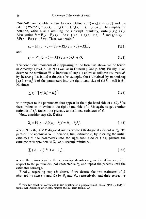
56 T. Amemiya, Tobit models: A survey
moments can be obtained as follows. Define z;(j) = s,(k,) - q(j) and the (K- 1)-vector z, = [z,(l) ,..., zi(k, - l), zi(ki+ 1) ,..., z,(K)]‘. To simplify the notation, write z, as z omitting the subscript. Similarly, write y,(k,) as y. Also, define R = E(y - Ey)(z - Et)‘: [E(z - Ez)(z - Ez)‘]-’ and Q = Vy - R&z - Ez)(y - Ey)‘. Then, we obtain*’
and
CL, = E( y]z > 0) = Ey + RE( z]z > 0) - REz, (162)
a,* = I”( y]z > 0) = RV( zlz > 0) R’ + Q. (163)
The conditional moments of z appearing in the formulae above can be found in Amemiya (1974, p. 1002) as well as in Duncan (1980, p. 850). Finally, I can describe the nonlinear WLS iteration of step (1) above as follows: Estimate CI, by inserting the initial estimates (for example, those obtained by minimizing [~~(mk&e~,]2) of the parameters into the right-hand side of (163) - call it 6:.
064)
with respect to the parameters that appear in the right-hand side of (162). Use these estimates to evaluate the right-hand side of (163) again to get another estimate of u,‘. Repeat the process, to yield new estimates of fl.
Now, consider step (2). Define
2, = E( w, - P,)( w,-P,)‘=D,-P,P,‘, (165)
where D, is the K x K diagonal matrix whose k th diagonal element is P,k. To perform the nonlinear WLS iteration, first, estimate .Zj by inserting the initial estimates of the parameters into the right-hand side of (165) (denote the estimate thus obtained as zi) and, second, minimize
(166)
where the minus sign in the superscript denotes a generalized inverse, with respect to the parameters that characterize Pi, and repeat the process until the estimates converge.
Finally, regarding step (3) above, if we denote the two estimates of p obtained by step (1) and (2) by pi and R,, respectively, and their respective
27These two equations correspond to two equations in a proposition of Duncan (1980, p. 851). It seems that Duncan inadvertently omitted the last term from (162).

T. Amemiya, Tobit models: A survey 51
asymptotic variance-covariance matrices2* by Vi and V,, the optimal linear combination of the two estimates is given by (Vi- ’ + V2- ‘) - ‘VI- ‘fi, + (VI- ’ + V2- ‘) -‘V,- ‘b2. This final estimator is asymptotically not fully efficient, how- ever. To see this, suppose the regression coefficients of (158) and (159) differ: call them /3i and h2, say. Then, by a result of Amemiya (1976), we know that fil is an asymptotically efficient estimator of &. However, as I have indicated in section 4.4, b2 is not. So a weighted average of the two could not be asymptotically efficient.
Dubin and McFadden (1980) used a similar model to Duncan’s in their study of the joint determination of the choice of electric appliances and the consumption of electricity. In their model, s,(k) may be interpreted as the utility of the i th family when they use the k th portfolio of appliances, and y,(k) as the consumption of electricity for the ith person holding the kth portfolio. The estimation method is essentially similar to Duncan’s. The main difference is that Dubin and McFadden assume that the error terms of (158) and (159) are distributed as Type I extreme value distribution and hence the P part of (161) is multinomial logit [cf. Amemiya (1981, p. 1516)].
References
Adams, J.D., 1980, Personal wealth transfers, Quarterly Journal of Economics 95, 159-179. Amemiya, T., 1973, Regression analysis when the dependent variable is truncated normal,
Econometrica 41, 997-1016. Amemiya, T., 1974a, A note on a Fair and JaKee model, Econometrica 42, 759-762. Amemiya, T., 1974b, Multivariate regression and simultaneous equation models when the depen-
dent variables are truncated normal, Econometrica 42, 999-1012. Amemiya, T., 1976, The maximum likelihood, the minimum &i-square and the nonlinear weighted
leasted-squares in the general qualitative response model, Journal of the American Statistical Association 71, 347-351.
Amemiya, T., 1978, The estimation of a simultaneous equation generalized probit model, Econometrica 46.1193-1205.
Amemiya, T., 1979, The estimation of a simultaneous-equation Tobit model, International Economic Review 20,169-181.
Amemiya, T., 1981a, Nonlinear regression models, Technical report no. 330 (IMSSS, Stanford University, Stanford, CA).
Amemiya, T., 1981b, Qualitative response models: A survey, Journal of Economic Literature 19, 1483-1536.
Amemiya, T., 1982, A comparison of the Amemiya GLS and the Lee-Maddala-Trost G2SLS in a simultaneous-equations Tobit model, Mimeo. (Rhodes Associates, Palo Alto, CA).
Amemiya, T. and M. Boskin, 1974, Regression analysis when the dependent variable is truncated lognormal, with an application to the determinants of the duration of welfare dependency, International Economic Review 15, 485-496.
Arabmazar, A. and P. Schmidt, 1981, Further evidence on the robustness of the Tobit estimator to heteroscedasticity, Journal of Econometrics 17, 253-258.
Arabmazar, A. and P. Schmidt, 1982, An investigation of the robustness of the Tobit estimator to non-normality, Econometrica 50,1055-1063.
2sThese matrices can be obtained by a standard procedure. See, for example, Amemiya (1981). The matrices must be evaluated at some consistent estimates; either /?, or a, will do

58 T. Amemiya, Tobir models: A survey
Ashenfelter, 0. and J. Ham, 1979, Education, unemployment, and earnings, Journal of Political Economy 87, S99-S116.
Bartholomew, D.J., 1973, Stochastic models for social processes, 2nd ed. (Wiley, New York). Borjas, G.J. and S. Rosen, 1980, Income prospects and job mobility of young men, Research in
Labor Economics 3,159-181. Chung, C.F. and A.S. Goldberger, 1982, Proportional projections in limited dependent variable
models, Mimeo. (University of Wisconsin, Madison, WI). Cragg, J.G., 1971, Some statistical models for limited dependent variables with application to the
demand for durable goods, Econometrica 39, 829-844. Dagenais, M.G., 1969, A threshold regression model, Econometrica 37, 193-203. Dagenais, M.G., 1975, Application of a threshold regression model to household purchases of
automobiles. Review of Economics and Statistics 57, 275-285. Dempster, A.P., N.M. Laird and D.B. Rubin, 1977, Maximum likelihood from incomplete data via
the EM algorithm, Journal of Royal Statistical Society B 39, l-38 (with discussion). Dubin. J.A. and D. McFadden, 1980, An econometric analysis of residential electric appliance
holdings and consumption, Mimeo. (MIT, Cambridge, MA). Dudley, L. and C. Montmarquette, 1976, A model of the supply of bilateral foreign aid, Amencan
Economic Review 66.132-142. Duncan, G.M., 1980, Formulation and statistical analysis of the mixed, continuous/discrete
dependent variable model in classical production theory, Econometrica 48, 839-852. Fair, R.C., 1978, A theory of extramarital affairs, Journal of Political Economy 86, 45-61. Fair, R.C. and D.M. Jatfee, 1972, Methods of estimation for markets in disequilibrium,
Econometrica 40,497-514. Flinn, C.J. and J.J. Heckman, 1982, Models for the analysis of labor force dynamics, Working
paper no. 857 (NBER, Cambridge, MA). Goldberger, A..%, 1964, Econometric theory (Wiley, New York). Goldberger, AS., 1980, Abnormal selection bias, SSRI workshop series no. 8006 (University of
Wisconsin, Madison, MA). Goldberger, A.S., 1981, Linear regression after selection, Journal of Econometrics 15, 357-366. Gourieroux. C.. J.J. Laffont and A. Monfort. 1980. Coherencv conditions in simultaneous linear
equation models with endogenous switching regimes, Econometrica 48,675-695. Greene, W.H., 1981, On the asymptotic bias of the ordinary least squares estimator of the Tobit
model, Econometrica 49,505-513. Greene, W.H., 1983, Estimation of limited dependent variable models by ordinary least squares
and the method of moments, Journal of Econometrics 21, 195-212. Gronau. R.. 1973. The effects of children on the housewife’s value of time, Journal of Political
Economy 81, S168-S199. Gronau, R., 1974, Wage comparisons: A selectivity bias, Journal of Political Economy 82,
1119-1143. Hartley, H.O., 1958, Maximum likelihood estimation from incomplete data, Biometrics 14,
174-194. Hartley, M.J., 1976a, The estimation of markets in disequilibrium: The fixed supply case,
International Economic Review 17,687-699. Hartley, M.J., 1976b, Estimation of the Tobit model by nonlinear least squares methods,
Discussion paper no. 373 (SUNY, Buffalo, NY). Hartley, M.J., 1976c, The Tobit and probit models: Maximum likelihood estimation by ordinary
least squares, Discussion paper no. 374 (SUNY, Buffalo, NY). Hausman, J.A., 1978, Specification tests in econometrics, Econometrica 46, 1251-1271. Hausman, J.A. and D.A. Wise, 1976, The evaluation of results from truncated samples: The New
Jersey income maintenance experiment, Annals of Economic and Social Measurement 5, 421-445.
Hausman, J.A. and D.A. Wise, 1977, Social experimentation, truncated distributions, and efficient estimation, Econometrica 45, 919-938.
Hausman, J.A. and D.A. Wise, 1979, Attrition bias in experimental and panel data: The Gary income maintenance experiment, Econometrica 47,455-473.
Heckman, J.J., 1974, Shadow prices, market wages, and labor supply, Econometrica 42, 679-693. Heckman, J.J., 1976a, The common structure of statistical models of truncation, sample selection

T. Amemiya, Tobit models: A survey 59
and limited dependent variables and a simple estimator for such models, Annals of Economic and Social Measurement 5, 475-492.
Heckman, J.J., 1976b, Simultaneous equations models with continuous and discrete endogenous variables and structural shifts, in: S.M. Goldfeld and R.E. Quandt, eds., Studies in nonlinear estimation (Ballinger, Cambridge, MA).
Heckman, J.J., 1978, Dummy endogenous variables in a simultaneous equation system, Econometrica 46.931-960.
Heckman, J.J., 1979, Sample selection bias as a specification error, Econometrica 47, 153-161. Heckman, J.J. and T.E. MaCurdy, 1980, A life cycle model of female labor supply, Review of
Economic Studies 47, 47-74. Huang, D.S., 1964, Discrete stock adjustment: The case of demand for automobiles, International
Economic Review 5,46-62. Hurd, M., 1979, Estimation in truncated samples when there is heteroscedasticity, Journal of
Econometrics 11, 247-258. Johnson, N.L. and S. Kotz, 1970, Continuous univariate distributions 1 (Houghton MiWin, Boston,
MA). Judge, N.L., W.E. Griffiths, R.C. Hill and T.C. Lee, 1980, Theory and practice of econometrics
(Wiley, New York). Kalbfleish, J.G. and R.L. Prentice, 1980, The statistical analysis of failure time data (Wiley, New
York). Keeley, M.C., P.K. Robins, R.G. Spiegelman and R.W. West, 1978, The estimation of labor supply
models using experimental data, American Economic Review 68, 873-887. Kenny, L.W., L.F. Lee, G.S. Maddala and R.P. Trost, 1979, Returns to college education: An
investigation of self-selection bias based on the project talent data, International Economic Review 20, 775-789.
Kotlikoff, L.J., 1979, Testing the theory of social security and life cycle accumulation, American Economic Review 69, 396-410.
Lancaster, T., 1979, Econometric methods for the duration of unemployment, Econometrica 47, 939-956.
Lee, L.F., 1977, Estimation of a modal choice model for the work journey with incomplete observations, Mimeo. (Department of Economics, University of Minnesota, Minneapolis, MN).
Lee, L.F., 1978, Unionism and wage rates: A simultaneous equations model with qualitative and limited dependent variables, International Economic Review 19,415-433.
Lee, L.F., 1979, Mixed logit and fully recursive logit models, Economics Letters 3, 363-368. Lee, L.F., 1981, Simultaneous equations models with discrete and censored variables, in: CF.
Manski and D. McFadden, eds., Structural analysis of discrete data with econometric applica- tions (MIT Press, Cambridge, MA).
Lee, L.F., 1982, Some approaches to the correction of selectivity bias, Review of Economic Studies 49, 355-372.
Lee, L.F., G.S. Maddala and R.P. Trost, 1980, Asymptotic covariance matrices of two-stage Probit and two-stage Tobit methods for simultaneous equations models with selectivity, Econometrica 48,491-503.
Lee, L.F. and R.P. Trost, 1978, Estimation of some limited dependent variable models with application to housing demand, Journal of Econometrics 8, 357-382.
Maddala, G.S., 1977, Econometrics (McGraw-Hill, New York). Maddala, G.S., 1980, Disequilibrium, self-selection and switching models, Social Science working
paper no. 303 (California Institute of Technology, Pasadena, CA). Maddala, G.S., 1983, Limited-dependent and qualitative variables in econometrics (Cambridge
University Press, Cambridge). Maddala, G.S. and F.D. Nelson, 1974, Maximum likelihood methods for models of markets in
disequilibrium, Econometrica 42,1013-1030. Miller, R., 1981, Survival analysis (Wiley, New York). Nakamura, A. and M. Nakamura, 1981, A comparison of the labor force behavior of married
women in the United States and Canada, with special attention to the impact of income taxes, Econometrics 49.451-489.
Nakamura, M., A. Nakamura and D. Cullen, 1979, Job opportunities, the offered wage, and the labor supply of married women, American Economic Review 69, 787-805.

60 T. Amemiya, Tobit models: A survey
Nelson, F.D., 1977, Censored regression models with unobserved, stochastic censoring thresholds, Journal of Econometrics 6, 309-327.
Nelson, F.D., 1981, A test for misspecification in the censored normal model, Econometrica 49, 1317-1329.
Nelson, F.D. and L. Olson, 1978, Specification and estimation of a simultaneous-equation model with limited dependent variables, International Economic Review 19, 695-709.
Olsen, R.J., 1978a, Note on the uniqueness of the maximum likelihood estimator for the Tobit model, Econometrica 46, 1211-1215.
Olsen, R.J., 1978b, Comment on ‘The effect of unions on earnings and earnings on unions: A mixed logit approach’, International Economic Review 19, 259-261.
Olsen, R.J., 1980, A least squares correction for selectivity bias, Econometrica 48, 1815-1820. Paarsch, H.J., 1984, A Monte Carlo comparison of estimators for censored regression models,
Journal of Econometrics, this issue. Poirier, D.J., 1978, The use of the Box-Cox transformation in limited dependent variable models,
Journal of the American Statistical Association 73, 284-287. Powell, J.L., 1981, Least absolute deviations estimation for censored and truncated regression
models, Technical report no. 356 (IMSSS, Stanford University, Stanford, CA). Powell, J.L., 1983, Asymptotic normality of the censored and truncated least absolute deviations
estimators, Technical report no. 395 (IMSSS, Stanford University, Stanford, CA). Quandt, R.E., 1982, Econometric disequilibrium models, Econometric Reviews 1, l-63. Rao, CR., 1973, Linear statistical inference and its application, 2nd ed. (Wiley, New York). Ray, E.J., 1981, The determinants of tariff and nontariff trade restrictions in the United States,
Journal of Political Economy 89, 105-121. Reece, W.S., 1979, Charitable contributions: The new evidence on household behavior, American
Economic Review 69, 142-151. Roberts, R.B., G.S. Maddala and G. Enholm, 1978, Determinants of the requested rate of return
and the rate of return granted in a formal regulatory process, Bell Journal of Economics 9, 611-621.
Robinson, P.M., 1982a, On the asymptotic properties of estimators of models containing limited dependent variables, Econometrica 50,27-41.
Robinson, P.M., 1982b, Analysis of time series from mixed distributions, Annals of Statistics 10, 915-925.
Rosenzweig, M.R., 1980, Neoclassical theory and the optimizing peasant: An econometric analysis of market family labor supply in a developing country, Quarterly Journal of Economics 94, 31-55.
Rosett, R.N., 1959, A statistical model of friction in economics, Econometrica 27, 263-267. Rosett, R.N. and F.D. Nelson, 1975, Estimation of the two-limit probit regression model,
Econometrica 43,141-146. Schmee, J. and G.J. Hahn, 1979, A simple method for regression analysis with censored data,
Technometrics 21, 417-432. Schmidt, P., 1978, Estimation of a simultaneous equations model with jointly dependent continu-
ous and qualitative variables: The union-earnings question revisited, International Economic Review 19, 453-465.
Schmidt, P. and R.P. Strauss, 1976, The effect of unions on earnings and earnings on union: A mixed logit approach, International Economic Review 17, 204-212.
Shishko, R. and B. Rostker, 1976, The economics of multiple job holding, American Economic Review 66,298-308.
Singer, B. and S. Spilerman, 1976, Some methodological issues in the analysis of longitudinal surveys, Annals of Economic and Social Measurement 5,447-474.
Stapleton, D.C. and D.J. Young, 1981, Censored normal regression with measurement error on the dependent variable, Discussion paper no. 81-30 (Department of Economics, University of British Columbia, Vancouver).
Stephenson, S.P. and J.F. McDonald, 1979, Disaggregation of income maintenance impacts on family earnings, Review of Economics and Statistics 61, 354-360.
Tobin, J., 1958, Estimation of relationships for limited dependent variables, Econometrica 26, 24-36.

T. Amemiya, Tobit models: A survey 61
Tomes, N., 1981, The family, inheritance, and the intergenerational transmission of inequality, JournaJ of Political Economy 89,928-958.
Tuma, N.B., M.T. Hannan and L.P. Groeneveld, 1979, Dynamic analysis of event histories, American Journal of Sociology 84, 820-854.
Tuma, N.B. and P.K. Robins, 1980, A dynamic model of employment behavior: An application to the Seattle and Denver income maintenance experiments, Econometrica 48, 1031-1052.
Wales, T.J. and A.D. Woodland, 1980, Sample selectivity and the estimation of labor supply functions, International Economic Review 21, 437-468.
Warren, R.S. and R.P. Strauss, 1979, A mixed logit model of the relationship between unionization and right-to-work legislation, Journal of Political Economy 87, 648-655.
Westin, R.B. and P.W. Gillen, 1978, Parking location and transit demand, Journal of Econometrics 8, 75-101.
White, H., 1980, A heteroscedasticity-consistent covariance matrix estimator and a direct test for heteroscedasticity, Econometrica 48, 817-838.
Wiggins, S.N., 1981, Product quality regulation and new drug introductions: Some new evidence from the 1970’s. Review of Economics and Statistics 63, 615-619.
Willis, R.J. and S. Rosen, 1979, Education and self-selection, Journal of Political Economy 87, S7-S36.
Witte, A.D., 1980, Estimating the economic model of crime with individual data, Quarterly Journal of Economics 94, 57-84.
Wu, C.F.J., 1983, On the convergence properties of the EM algorithm, Annals of Statistics 11, 95-103.
Wu, D.M., 1965, An empirical analysis of household durable goods expenditure, Econometrica 33, 761-780.