arX

iv:1

610.

0455

1v4

[cs

.SD

] 2

3 A

pr 2

017

Tonal consonance parameters link microscopic and

macroscopic properties of music exposing a hidden order

in melody

J. E. Useche 1 R. G. Hurtado2

Abstract

Consonance is related to the perception of pleasantness arising from a combination of sounds and has been

approached quantitatively using mathematical relations, physics, information theory, and psychoacoustics.

Tonal consonance is present in timbre, musical tuning, harmony, and melody, and it is used for conveying

sensations, perceptions, and emotions in music. It involves the physical properties of sound waves and is used

to study melody and harmony through musical intervals and chords. From the perspective of complexity,

the macroscopic properties of a system with many parts frequently rely on the statistical properties of its

constituent elements. Here we show how the tonal consonance parameters for complex tones can be used

to study complexity in music. We apply this formalism to melody, showing that melodic lines in musical

pieces can be described in terms of the physical properties of melodic intervals and the existence of an

entropy extremalization principle subject to psychoacoustic macroscopic constraints with musical meaning.

This result connects the human perception of consonance with the complexity of human creativity in music

through the physical properties of the musical stimulus.

Keywords: Consonance; Entropy; Melody; Music.

1. Introduction

Pythagoras found that two sounds emitted simultaneously by vibrating strings of equal tension and densityproduce a pleasant sensation when the ratio between their lengths (and hence their fundamental frequencies)corresponds to the ratio between two small natural numbers n/m [1, 2, 3]. This sensation is formally definedas consonance, and it is present in melody, harmony, timbre, and musical tuning [2, 3, 4]. Many authors relateconsonance to conveying musical information as emotions and meaning [5, 6, 7, 8]. From the perspective ofthe nature of tonality, consonance and dissonance give rise to emotions through tension and relaxation [6] inpassages from satisfaction to dissatisfaction and again to satisfaction [7, 9].A starting point for studying consonance in psychoacoustics is the superposition of pure tones with differentfrequencies [1, 10, 11]. Hermann von Helmholtz found that the consonance level of pairs of simultaneous puretones is related to the beats produced by fluctuations in the peak intensity of the resulting sound waves [10];specifically, the perception of dissonance is proportional to the perception of roughness due to rapid beats [3].Musical instruments produce complex tones that can be represented by the superposition of several pure tones.The corresponding set of frequencies with their amplitudes is called the spectrum which strongly characterizesthe timbre of a musical instrument [1]. For complex tones, Helmholtz inferred that the superposition of spectrumcomponents with close frequencies is related to the perception of dissonance [10, 3].After Helmholtz, Reinier Plomp and Willem Levelt reported that the transition range between consonance anddissonance is related to a critical bandwidth that depends on the frequency difference of the correspondingsound waves [12]. This approach to consonance is known as tonal or sensory, because it depends on the physicalproperties of the stimulus, regardless of the cultural context of the listener [13].William Sethares assigned a level of tonal consonance to timbre using the spectrum of the emitted sound andconnected timbre with musical tuning [4, 14]. Musical tuning refers to adjusting a set of pitches to a musicalscale using a fixed pitch of reference. Pitch is a subjective quality of sound that judges its height and dependsstrongly on the lowest frequency of the spectrum, the fundamental frequency [1], and usually a musical scale isa set of mathematical relations among the fundamental frequencies of pitches. Pairs of pitches in a musical scaledefine musical intervals of size L given by the number of pitches between them. In musical theory, the level ofconsonance assigned to a musical interval usually depends on its size (and hence the fundamental frequency ratioof its pitches) [15]. Since musicians tend to apply the same rules for judging the consonance level of simultaneousand successive pitches (harmonic and melodic intervals respectively), and the short-term persistence of pitch inauditoriums may give rise to consonance sensations for successive pitches [3], then tonal consonance is suitablefor analyzing both harmony and melody.

1jeusecher@unal.edu.co2Corresponding author. Postal address: Carrera 30 No. 45-03, Departamento de Fısica, Universidad Nacional de Colombia,

Bogota, Colombia. rghurtadoh@unal.edu.co

1

In this paper we will study the consonance properties of melody, defined by the New Grove Dictionary of Musicand Musicians as “pitched sounds arranged in musical time in accordance with given cultural conventions andconstraints” [16]. An alternative definition that encompasses music and speech was given by Aniruddh Patel:“an organized sequence of pitches that conveys a rich variety of information to a listener” [17].With respect to the statistical properties of melody, George Kingsley Zipf studied the frequency of occurrenceof melodic intervals in masterpieces of Western tonal music. Melodic intervals can be played in an ascendantor a descendant manner, and Zipf reported that the frequency of occurrence in both cases is almost inverselyproportional to their size [18]. Melodies tend to meander around a central pitch range, and for many cultures anasymmetry emerges in this meandering, in the sense that large melodic intervals are more likely to ascend andsmall melodic intervals are more likely to descend [19]. A more recent study proposes long-tailed Levy-stabledistributions to model the probability distribution of melodic intervals as a function of their size [20]. The useof physical quantities to represent melodic intervals has generated a new approach to analyze melody obtainingexponential and power law probability distributions with good experimental determination coefficients [21].These studies show signs of complexity in melody but don’t define a formal relation between the size of musicalintervals and consonance. Other studies also show that musical pieces present complexity as scale-free patternsin the fluctuations of loudness [22], rhythm synchronization [23], and pitch behavior in melody [22], as well as inthe connectivity properties of complex networks representing successive notes of musical pieces [24]. Regardingconsonance, a recent study found scale-free patterns in the consonance fluctuations associated with harmony[25].From the perspective of information theory, Gungor Gunduz and Ufuk Gunduz measured the probability ofoccurrence of musical notes during the progress of melodies and found that entropy grows up to a limiting valuesmaller than the entropy of a random melody [26].In this paper, we show how tonal consonance parameters for complex tones can be used to study complexity inmusic, using a more general quantity than the size of the musical interval, because it distinguishes the level ofconsonance and the position in the register of a musical interval. In order to demonstrate the usefulness of thisformalism, we apply it to melody through the study of twenty melodic lines from seven masterpieces of Westerntonal music. We also develop a theoretical model based on relative entropy extremalization, in agreement withthe qualitative definitions of melody, for reproducing the main features of experimental results and linkingthe microscopic tonal consonance properties of melodic intervals, including timbre, with the macroscopic onesstemming from their organization in real melodic lines.

2. Tonal consonance parameters for pure and complex tones

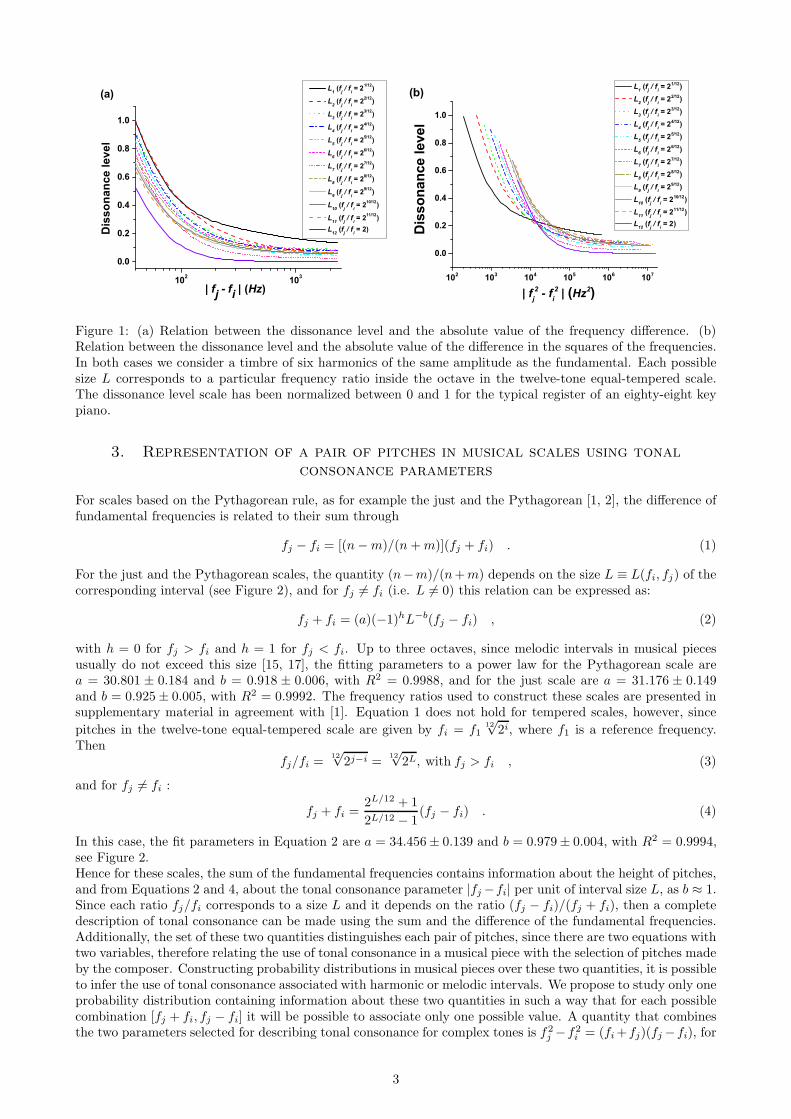
The method for determining the tonal consonance of pure tones is related to the beats produced by the super-position of two sinusoidal signals with different frequencies, fi and fj. The superposition of pure tones varies intime with a rapid frequency (fi+fj)/2 modulated by a slow one |fj−fi|/2. The beats produced by fluctuationsin the peak intensity of sound waves occur with a frequency |fj−fi|, and this phenomenon is independent of thedifferences in amplitude and phase between the two pure tones (see supplementary material) for details). Thisresult indicates that the main contribution of tonal consonance for pure tones are their frequency components.The approach of Plomp and Levelt to tonal consonance of complex tones is independent of musical scales, andthey found that an interval of a given size L might be more or less consonant depending on its timbre andlocation in the register and that this variation through the register is continuous and smooth [12]. They usedtwo quantities for parametrizing the tonal consonance level of complex tones: the lowest fundamental frequencyof the pair of pitches and the ratio between the fundamental frequencies fj/fi [12]. This set of parameters isequivalent to one with the same ratio fj/fi and the absolute value of the difference between the fundamentalfrequencies |fj − fi| (see supplementary material for details), which will be the equivalent parameter in com-parison with pure tones. We use the William Sethares formalism to reproduced these curves in the case of aparticular timbre (see supplementary material for details).Figure 1a shows the tonal consonance curves in the case of simultaneous pitches (which for musicians can also beused in the case of successive pitches) for a timbre of six harmonics of the same amplitude as the fundamental,in the case of the frequency ratios of the twelve-tone equal-tempered scale within an octave. In this figure, wecan see that an interval of a certain size L is more consonant in the middle part of the registry than in thelowest part. For all sizes, these curves fit to a second-order exponential decay function with a coefficient ofdetermination R2 = 0.99.

2

102 103

0.0

0.2

0.4

0.6

0.8

1.0

(a)D

isso

nanc

e le

vel

| fj - fi | (Hz)

L1 (fj / fi = 21/12)

L2 (fj / fi = 22/12)

L3 (fj / fi = 23/12)

L4 (fj / fi = 24/12)

L5 (fj / fi = 25/12)

L6 (fj / fi = 26/12)

L7 (fj / fi = 27/12)

L8 (fj / fi = 28/12)

L9 (fj / fi = 29/12)

L10 (fj / fi = 210/12)

L11 (fj / fi = 211/12) L12 (fj / fi = 2)

102 103 104 105 106 107

0.0

0.2

0.4

0.6

0.8

1.0

Dis

sona

nce

leve

l

| f 2j - f 2

i | (Hz2)

L1 (fj / fi = 21/12) L2 (fj / fi = 22/12) L3 (fj / fi = 23/12) L4 (fj / fi = 24/12) L5 (fj / fi = 25/12) L6 (fj / fi = 26/12) L7 (fj / fi = 27/12) L8 (fj / fi = 28/12) L9 (fj / fi = 29/12) L10 (fj / fi = 210/12) L11 (fj / fi = 211/12) L12 (fj / fi = 2)

(b)

Figure 1: (a) Relation between the dissonance level and the absolute value of the frequency difference. (b)Relation between the dissonance level and the absolute value of the difference in the squares of the frequencies.In both cases we consider a timbre of six harmonics of the same amplitude as the fundamental. Each possiblesize L corresponds to a particular frequency ratio inside the octave in the twelve-tone equal-tempered scale.The dissonance level scale has been normalized between 0 and 1 for the typical register of an eighty-eight keypiano.

3. Representation of a pair of pitches in musical scales using tonal

consonance parameters

For scales based on the Pythagorean rule, as for example the just and the Pythagorean [1, 2], the difference offundamental frequencies is related to their sum through

fj − fi = [(n−m)/(n+m)](fj + fi) . (1)

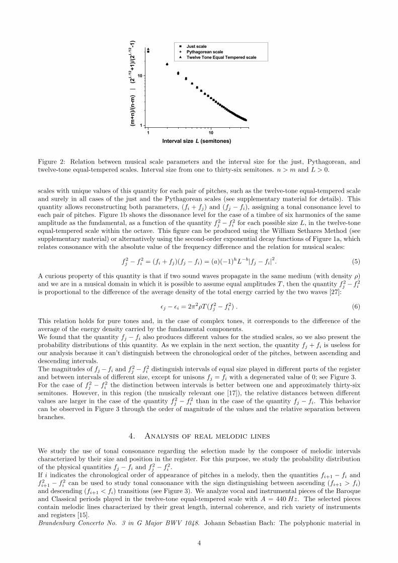
For the just and the Pythagorean scales, the quantity (n−m)/(n+m) depends on the size L ≡ L(fi, fj) of thecorresponding interval (see Figure 2), and for fj 6= fi (i.e. L 6= 0) this relation can be expressed as:

fj + fi = (a)(−1)hL−b(fj − fi) , (2)

with h = 0 for fj > fi and h = 1 for fj < fi. Up to three octaves, since melodic intervals in musical piecesusually do not exceed this size [15, 17], the fitting parameters to a power law for the Pythagorean scale area = 30.801 ± 0.184 and b = 0.918 ± 0.006, with R2 = 0.9988, and for the just scale are a = 31.176 ± 0.149and b = 0.925± 0.005, with R2 = 0.9992. The frequency ratios used to construct these scales are presented insupplementary material in agreement with [1]. Equation 1 does not hold for tempered scales, however, since

pitches in the twelve-tone equal-tempered scale are given by fi = f112√2i, where f1 is a reference frequency.

Thenfj/fi =

12√2j−i =

12√2L, with fj > fi , (3)

and for fj 6= fi :

fj + fi =2L/12 + 1

2L/12 − 1(fj − fi) . (4)

In this case, the fit parameters in Equation 2 are a = 34.456± 0.139 and b = 0.979± 0.004, with R2 = 0.9994,see Figure 2.Hence for these scales, the sum of the fundamental frequencies contains information about the height of pitches,and from Equations 2 and 4, about the tonal consonance parameter |fj−fi| per unit of interval size L, as b ≈ 1.Since each ratio fj/fi corresponds to a size L and it depends on the ratio (fj − fi)/(fj + fi), then a completedescription of tonal consonance can be made using the sum and the difference of the fundamental frequencies.Additionally, the set of these two quantities distinguishes each pair of pitches, since there are two equations withtwo variables, therefore relating the use of tonal consonance in a musical piece with the selection of pitches madeby the composer. Constructing probability distributions in musical pieces over these two quantities, it is possibleto infer the use of tonal consonance associated with harmonic or melodic intervals. We propose to study only oneprobability distribution containing information about these two quantities in such a way that for each possiblecombination [fj + fi, fj − fi] it will be possible to associate only one possible value. A quantity that combinesthe two parameters selected for describing tonal consonance for complex tones is f2

j −f2i = (fi+fj)(fj −fi), for

3

1 101

10

Just scale Pythagorean scale Twelve Tone Equal Tempered scale

(m+n

)/(n-

m)

|

(2L

/12 +1

)/(2L

/12 -1

)Interval size L (semitones)

Figure 2: Relation between musical scale parameters and the interval size for the just, Pythagorean, andtwelve-tone equal-tempered scales. Interval size from one to thirty-six semitones. n > m and L > 0.

scales with unique values of this quantity for each pair of pitches, such as the twelve-tone equal-tempered scaleand surely in all cases of the just and the Pythagorean scales (see supplementary material for details). Thisquantity allows reconstructing both parameters, (fi + fj) and (fj − fi), assigning a tonal consonance level toeach pair of pitches. Figure 1b shows the dissonance level for the case of a timbre of six harmonics of the sameamplitude as the fundamental, as a function of the quantity f2

j − f2i for each possible size L, in the twelve-tone

equal-tempered scale within the octave. This figure can be produced using the William Sethares Method (seesupplementary material) or alternatively using the second-order exponential decay functions of Figure 1a, whichrelates consonance with the absolute value of the frequency difference and the relation for musical scales:

f2j − f2

i = (fi + fj)(fj − fi) = (a)(−1)hL−b|fj − fi|2. (5)

A curious property of this quantity is that if two sound waves propagate in the same medium (with density ρ)and we are in a musical domain in which it is possible to assume equal amplitudes T , then the quantity f2

j − f2i

is proportional to the difference of the average density of the total energy carried by the two waves [27]:

ǫj − ǫi = 2π2ρT (f2j − f2

i ) . (6)

This relation holds for pure tones and, in the case of complex tones, it corresponds to the difference of theaverage of the energy density carried by the fundamental components.We found that the quantity fj − fi also produces different values for the studied scales, so we also present theprobability distributions of this quantity. As we explain in the next section, the quantity fj + fi is useless forour analysis because it can’t distinguish between the chronological order of the pitches, between ascending anddescending intervals.The magnitudes of fj − fi and f2

j − f2i distinguish intervals of equal size played in different parts of the register

and between intervals of different size, except for unisons fj = fi with a degenerated value of 0; see Figure 3.For the case of f2

j − f2i the distinction between intervals is better between one and approximately thirty-six

semitones. However, in this region (the musically relevant one [17]), the relative distances between differentvalues are larger in the case of the quantity f2

j − f2i than in the case of the quantity fj − fi. This behavior

can be observed in Figure 3 through the order of magnitude of the values and the relative separation betweenbranches.

4. Analysis of real melodic lines

We study the use of tonal consonance regarding the selection made by the composer of melodic intervalscharacterized by their size and position in the register. For this purpose, we study the probability distributionof the physical quantities fj − fi and f2

j − f2i .

If i indicates the chronological order of appearance of pitches in a melody, then the quantities fi+1 − fi andf2i+1 − f2

i can be used to study tonal consonance with the sign distinguishing between ascending (fi+1 > fi)and descending (fi+1 < fi) transitions (see Figure 3). We analyze vocal and instrumental pieces of the Baroqueand Classical periods played in the twelve-tone equal-tempered scale with A = 440 Hz. The selected piecescontain melodic lines characterized by their great length, internal coherence, and rich variety of instrumentsand registers [15].Brandenburg Concerto No. 3 in G Major BWV 1048. Johann Sebastian Bach: The polyphonic material in

4

0 20 40 60 80

-4.0x103

-2.0x103

0.0

2.0x103

4.0x103

Interval size L (semitones)

f j - f

i (H

z)(a)

0 20 40 60 80

-2x107

-1x107

0

1x107

2x107

Interval size L (semitones)

f 2 j -

f 2 i (H

z2 )

(b)

Figure 3: Relation between the quantities fj − fi and f2j − f2

i and the interval size in semitones ((a) and (b)respectively) for the register of a typical eighty-eight key piano. These quantities distinguish intervals of equalsize played in different parts of the register and between intervals of different sizes. The upper branch comesfrom j = 88 (highest pitch) and i varies from 88 to 1. The tuning comes from the frequency relation for thetwelve-tone equal-tempered scale with A = 440Hz.

this concerto for eleven musical instruments (three violins, three violas, three cellos, violone, and harpsichord)makes it possible to assume that each instrument has a melodic motion.Missa Super Dixit Maria. Hans Leo Hassler: Polyphonic composition for four voices (soprano, contralto, tenorand bass).First movement of the Partita in A Minor BWV 1013. Johann Sebastian Bach: This piece has just one melodicline, for flute.Piccolo Concerto RV444. Antonio Vivaldi (arrangement by Gustav Anderson): We selected the piccolo melodicline because of its rich melodic content.Sonata KV 545. Wolfgang Amadeus Mozart: We selected the melodic line for the right hand of this pianosonata assuming that it drives the melodic content.Suite No. 1 in G Major BWV 1007 and Suite No. 2 in D Minor BWV 1008. Johann Sebastian Bach: Themelodic lines of these pieces written for cello have mainly successive pitches. In the case of the few simultaneouspitches, the continuation of the melodic lines was assumed in the direction of the highest pitch.First, we generated simplified MIDI files [24] in order to extract from the scores the probability distributionsof the quantities fi+1 − fi and f2

i+1 − f2i and the complementary cumulative distribution functions (CCDF) for

|fi+1 − fi| and |f2i+1 − f2

i |, which give information about the functional form of the probability distributions.Since the concept of chroma states that the consonance level of the unison is equivalent to the correspondingoctave [2] and the octave can be an ascending (fi+1/fi = 2/1) or a descending (fi+1/fi = 1/2) transition, thenfor our analysis we consider the unison as an ascending transition as well as a descending one. This meansthat we begin the bin count considering the bin box [0, x) for ascending transitions and the bin box (y, 0] fordescending transitions, where x and y are bin widths generated by the Sturges criterion in histograms. In ourexperimental analysis we found that the contribution of unisons is important for ascending transitions as well asfor descending ones. Furthermore, as we have different right hand limit and left hand limit when we approachto 0, we can’t take a bin around 0 containing ascending and descending transitions. Additionally, if we try todistribute the unisons between the ascending and the descending part, it procedure reduces the determinationcoefficient R2 in histograms [28] because we would be modifying the right hand and the left hand limits.In the cases of ascending transitions (fi+1 > fi), descending transitions (fi+1 < fi using |fi+1 − fi| and|f2

i+1 − f2i |), and the joint set of them (using |fi+1 − fi| and |f2

i+1 − f2i | for all transitions), the CCDF fit to

exponential functions for all sets with average determination coefficient R2 ≈ 0.99 with an standard deviationSD ≈ 0.01 (see supplementary material for details). Since the number of transitions in the studied melodic linesis at maximum one order of magnitude larger than the total number of possible transitions between pairs ofsuccessive pitches in the same ambitus (range between the lowest pitch and the highest one) and the number ofpossible transitions for any melodic line is finite independently of its length, then the probability distributionsmust be represented in histograms with bin width moderately dependent on the number of transitions. Theseconditions are satisfied by the Sturges criterion [29]. This analysis with histograms is important due to thetypical lengths of melodic lines in music.

5

Histograms for both quantities fit to exponential functions with the highest R2 for f2i+1 − f2

i with ascending

and descending transitions taken separately: for ascending transitions R2 = 0.987 with SD = 0.009 andfor descending ones R2 = 0.986 with SD = 0.016; see supplementary material for details. So we center ouranalysis on the quantity f2

i+1−f2i instead fi+1−fi, because this removes possible degenerations more efficiently,

produces better fits to exponential functions, and generates larger relative distances between different values(see supplementary material for details). In order to present ascending and descending transitions in the samehistogram, we merge the left and right branches of the distribution functions by defining the bin width as theaverage of the two bin widths. Then the probability distribution of f2

i+1 − f2i can be written as

P (ε) =

{

FH+ e−ε/GH

+ for ε > 0

FH− eε/G

H

− for ε < 0, (7)

where the notation ε emphasizes that these distributions are constructed over bins. In the case of the cumulativedistributions, we use CCDF for ascending transitions and complementary cumulative distribution functions fordescending ones (CDF). These choices allow conserving the same functional form as the probability distributions(this is possible due to the exponential behavior) but without the use of bins:

P (f2i+1 − f2

i ) =

{

FC+ e−(f2

i+1−f2i)/GC

+ for (f2i+1 − f2

i ) > 0

FC− e(f

2i+1−f2

i)/GC

− for (f2i+1 − f2

i ) < 0, (8)

the “.xlsx” file in supplementary material contains the values of FH+ , FH

− , GH+ , GH

− , FC+ , FC

− , GC+, G

C− of fits and

the determination coefficients R2. These probability distributions resemble the asymmetric Laplace probabilitydistribution with different amplitudes for positive and negative branches generating a discontinuity in the origin(Figure 4) [30].

Figure 4: General form of the probability distribution P (ε) and cumulative probability distribution P (f2i+1−f2

i ).In the symmetric case, P1 = P2 and α2 = α2.

Figure 5 shows the histogram of the probability distribution of ascending and descending transitions (includingunisons) in the case of the first movement of the Partita in A minor BWV 1013 as well as the bin degenerationfor the corresponding ambitus. To explain the effect of bin degeneration notice that the distance in Hz2 betweenpairs of differences f2

j − f2i for the twelve-tone equal-tempered scale varies in such a way that the number of

differences inside an arbitrary bin ε, its degeneracy, decreases when |f2j − f2

i | increases, and the probabilitydistribution is equivalent to the corresponding one of a random melodic line (see supplementary material). Thecomparison between the distributions of real melodic lines with those from bin degeneration for the correspondingambitus indicates that the scale contributes to the observed results but does not explain them. Additionally,the probability distribution for bin degeneration fits better to a power law function (R2 = 0.963) than to anexponential function (R2 = 0.934) (see supplementary material for details).

The quantitative difference between the probability distribution for a real melodic line and its correspondingrandom one gives information about the order introduced by the composer coming from the selection of successivepairs of pitches. A mathematical tool for comparing two probability distributions is the Kullback-Leiblerdivergence or relative entropy [31]

DKL =N∑

k=1

pk ln

(

pkqk

)

, (9)

where pk is the probability distribution for the real melodic line to be compared with the a priori distributionqk coming from the degeneration of the kth bin and that we associated with a random melodic line with thesame ambitus of the real one. N is the number of bins coming from the ambitus with N/2 bins for each branch.

6

-2x106 -1x106 0 1x106 2x106

1x10-3

1x10-2

1x10-1

Prob

ability

(Hz2)

Tempered scale First mov. Partita

Figure 5: Twelve-tone equal-tempered scale effect. Comparison between the probability distribution for the realmelodic line of the first movement of the Partita in A minor BWV 1013 by J. S. Bach and the correspondingbin degeneration for the same ambitus.

5. Statistical model

For modeling the system in an analogy to equilibrium statistical physics, we use the definitions of melody[16, 17] and the results obtained by G. Gunduz and U. Gunduz [26], assuming that the composer would have tocreate a melodic line among the richest ones in terms of the combination of successive pitches. This procedureis equivalent to minimizing the relative entropy (the closest pk to qk) with mathematical constraints containingrelevant musical information. The first constraint of the model comes from normalization. Since there are threekinds of different melodic intervals (ascending, descending, and unisons), then the normalization constraint isgiven by pa+pd+pu = 1, where pa is the probability of ascending intervals, pd is the probability of the descendingones and pu the probability of unisons. If pu is known, then pa and pd can be found from the normalizationconstraint and the asymmetry between ascending and descending intervals pa − pd. An equivalent alternativeis to use the normalization constraint and to measure from histograms the next two observables

pd + pu =

N/2∑

k=1

pk and pa + pu =

N∑

k=(N

2+1)

pk . (10)

Here∑N

k=1 pk = 1+pu in order to be consistent with the double count of unisons. This choice only changes theresult of the minimization problem (with respect to the normalized probability p∗k = pk

1+pu

) by the multiplication

of a positive constant (see supplementary material for details).The difference between the probability distributions of real melodic lines and their corresponding random onesleads to the second constraint. It comes from the selection made by the composer of the size and position inthe register of musical intervals, independently of whether they are ascending or descending ones, which can beassociated with the use of tonal consonance as follows. From Equation 2 with b ≈ 1 and assuming that each bink can be represented by the median of its extremes εk (in supplementary material we analyze this assumptionfor a typical case), since εk is linked with the interval size L and the tonal consonance parameter |fj − fi|, thenthe expected value of |ε| can be written (see supplementary material for details) as:

〈|ε|〉 =N∑

k=1

pk · |εk| = a

[

N∑

k=1

pk〈σ2/L〉k +N∑

k=1

pk〈|fj − fi|2/L〉k

]

, (11)

where σ2 is a variance associated with the size of intervals inside a bin. Using histograms, this is the bestestimation that we can make of 〈|ε|〉. The first term in the second line of Equation 11 is related to the dispersionof the size of the musical interval inside each bin and the second term to the location of intervals in the registerfor each bin. The location of musical intervals is measured in terms of the average of the frequency differences,which can be related to an average of tonal consonance using the tonal consonance curves for complex tones(see supplementary material for the details). In this model, the expected value 〈|ε|〉 is conserved, just as theexpected value of the energy in the canonical ensemble of statistical physics [32].In order to explore the nature of the quantity 〈|ε|〉, we consider the case in which each bin contains at maximumone possible transition. If we are in an equal amplitudes domain, then (see Equation 6)

〈|ε|〉 = 〈|f2p+1 − f2

p |〉 = |ǫ2p+1 − ǫ2p|/(2π2ρT ) , (12)

7

where |ǫ2p+1− ǫ2p| will be the expected value of the magnitude of the difference in the average density of the totalenergy carried by the two fundamental components of the sound waves. Furthermore, the analogous expressionof Equation 11 when each bin contains a maximum of one possible transition will be:

〈|ε|〉 = a

[

N∑

k=1

pk(fj − fi)

2k

Lk

]

= a

[

W∑

x=1

1

Lx

∑

h

pxh

|fj − fi|2xh

]

, (13)

where x runs from 1 to the total number of possible interval sizes W in the corresponding ambitus, h refersto the possible locations of musical intervals of size x in the register, and pxh

is the probability of finding aparticular interval of size x in the position h of the register inside the melodic line. In comparison with Equation11, the first term vanishes and the average disappears. Note that in Equation 13 we could split the expectedvalue into contributions of equal size L, so we can use the tonal consonance curves for complex tones to directlyrelate the absolute value of frequency difference with the dissonance level.We include the asymmetry in the selection of ascending and descending intervals as a third constraint. Thisasymmetry is present in the difference of the coefficients for the left and right branches in Equations 7 and8. First we analyze the continuity equation resulting from the fact that the second pitch of a transition is thefirst pitch of a successive transition. For a continuous segment of M successive pitches, the quantity δ for thissegment is defined as

δ = f2M − f2

1 =M−1∑

r=1

f2r+1 − f2

r , (14)

where r is a natural number that indicates the chronological order of appearance of pitches. The magnitude ofδ is smaller than or equal to the difference f2

max − f2min, given by the maximum and the minimum frequencies

in the ambitus of the melodic line. If we have G transitions and U continuous segments separated by rests in amelodic line, the expected value of f2

r+1 − f2r is

〈|f2r+1 − f2

r |〉 =1

G

U∑

v=1

δv . (15)

Melodic balance (melodies tend to meander around a central pitch range) and the continuity of musical phrasesare common properties of musical pieces, including those from the Baroque and Classical periods [15], leadingto values of 〈|f2

r+1 − f2r |〉 much smaller than those of 〈f2

r+1 − f2r 〉. Using histograms, the best estimation that

we can make of the expected value of Equation 15 is

〈ε〉 =N∑

k=1

pk · εk = −a

[

N/2∑

k=1

pk〈σ2/L〉k +N/2∑

k=1

pk〈|fj − fi|2/L〉k

]

+a

[

N∑

k=(N

2+1)

pk〈σ2/L〉k +N∑

k=(N

2+1)

pk〈|fj − fi|2/L〉k

]

.

(16)

Equation 16 is our last constraint and shows that 〈ε〉 is due to the asymmetry in the use of the size andposition in the register of ascending (positive terms) and descending (negative terms) intervals. Equations 11and 16 imply that unless there is an extremely unusual asymmetry between the use of ascending and descendingintervals, 〈ε〉 must be much smaller than 〈|ε|〉, a behavior that we noted in our experimental analysis (see ”.xlsx”file in supplementary material). Minimizing the relative entropy subject to the constraints in Equations 10, 11,and 16 produced the probability distribution [30] (see supplementary material for details)

pk =

(pd + pu)qke(−λ1|εk|−λ2εk)

N/2∑

m=1[qme(−λ1|εm|−λ2εm)]

for k ∈ [1, N/2]

(pa + pu)qke(−λ1|εk|−λ2εk)

N∑

m=(N

2+1)

[qme(−λ1|εm|−λ2εm)]

for k ∈ [N2 + 1, N ],

(17)

where λ1 and λ2 are the Lagrange multipliers for constraints 11 and 16, respectively. Using the expected values〈|ε|〉 and 〈ε〉 obtained from the empirical distributions for the selected melodic lines, and allowing less than 1.0%of error between the results from the statistical model and those of real data, we obtain the values for λ1 and λ2

(see ”.xlsx” file in supplementary material), with λ1 from one to two orders of magnitude larger than λ2. While

8

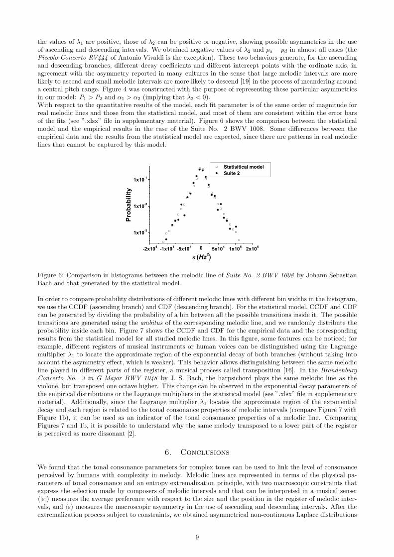
the values of λ1 are positive, those of λ2 can be positive or negative, showing possible asymmetries in the useof ascending and descending intervals. We obtained negative values of λ2 and pa − pd in almost all cases (thePiccolo Concerto RV444 of Antonio Vivaldi is the exception). These two behaviors generate, for the ascendingand descending branches, different decay coefficients and different intercept points with the ordinate axis, inagreement with the asymmetry reported in many cultures in the sense that large melodic intervals are morelikely to ascend and small melodic intervals are more likely to descend [19] in the process of meandering arounda central pitch range. Figure 4 was constructed with the purpose of representing these particular asymmetriesin our model: P1 > P2 and α1 > α2 (implying that λ2 < 0).With respect to the quantitative results of the model, each fit parameter is of the same order of magnitude forreal melodic lines and those from the statistical model, and most of them are consistent within the error barsof the fits (see ”.xlsx” file in supplementary material). Figure 6 shows the comparison between the statisticalmodel and the empirical results in the case of the Suite No. 2 BWV 1008. Some differences between theempirical data and the results from the statistical model are expected, since there are patterns in real melodiclines that cannot be captured by this model.

-2x105 -1x105 -5x104 0 5x104 1x105 2x105

1x10-3

1x10-2

1x10-1

(Hz2)

Prob

ability

Statisitical model Suite 2

Figure 6: Comparison in histograms between the melodic line of Suite No. 2 BWV 1008 by Johann SebastianBach and that generated by the statistical model.

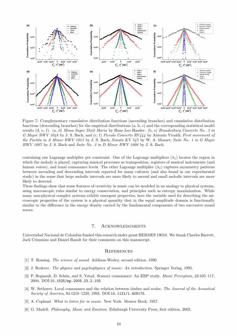
In order to compare probability distributions of different melodic lines with different bin widths in the histogram,we use the CCDF (ascending branch) and CDF (descending branch). For the statistical model, CCDF and CDFcan be generated by dividing the probability of a bin between all the possible transitions inside it. The possibletransitions are generated using the ambitus of the corresponding melodic line, and we randomly distribute theprobability inside each bin. Figure 7 shows the CCDF and CDF for the empirical data and the correspondingresults from the statistical model for all studied melodic lines. In this figure, some features can be noticed; forexample, different registers of musical instruments or human voices can be distinguished using the Lagrangemultiplier λ1 to locate the approximate region of the exponential decay of both branches (without taking intoaccount the asymmetry effect, which is weaker). This behavior allows distinguishing between the same melodicline played in different parts of the register, a musical process called transposition [16]. In the Brandenburg

Concerto No. 3 in G Major BWV 1048 by J. S. Bach, the harpsichord plays the same melodic line as theviolone, but transposed one octave higher. This change can be observed in the exponential decay parameters ofthe empirical distributions or the Lagrange multipliers in the statistical model (see ”.xlsx” file in supplementarymaterial). Additionally, since the Lagrange multiplier λ1 locates the approximate region of the exponentialdecay and each region is related to the tonal consonance properties of melodic intervals (compare Figure 7 withFigure 1b), it can be used as an indicator of the tonal consonance properties of a melodic line. ComparingFigures 7 and 1b, it is possible to understand why the same melody transposed to a lower part of the registeris perceived as more dissonant [2].

6. Conclusions

We found that the tonal consonance parameters for complex tones can be used to link the level of consonanceperceived by humans with complexity in melody. Melodic lines are represented in terms of the physical pa-rameters of tonal consonance and an entropy extremalization principle, with two macroscopic constraints thatexpress the selection made by composers of melodic intervals and that can be interpreted in a musical sense:〈|ε|〉 measures the average preference with respect to the size and the position in the register of melodic inter-vals, and 〈ε〉 measures the macroscopic asymmetry in the use of ascending and descending intervals. After theextremalization process subject to constraints, we obtained asymmetrical non-continuous Laplace distributions

9

-2x105 -1x105 -5x104 0 5x104 1x105 2x105

1x10-3

1x10-2

1x10-1

Cum

ulat

ive

Prob

abili

ty

f 2i+1- fi

2 (Hz2)

Soprano Contralto Tenor Bass

(a)

-2x105 -1x105 0 1x105 2x105

1x10-3

1x10-2

1x10-1

f 2i+1- fi

2 (Hz2)

Cum

ulat

ive

Prob

abili

ty

Violin 1 Viola 1 Cello 1 Harpsichord Violone

(b)

-2x106-2x106-1x106-5x105 0 5x105 1x106 2x106 2x106

1x10-3

1x10-2

1x10-1

Cum

ulat

ive

Prob

abili

ty

f 2i+1- fi

2 (Hz2)

Piccolo concerto First mov. Partita Mozart sonata Suite 1 Suite 2

(c)

-2x105 -1x105 -5x104 0 5x104 1x105 2x105

1x10-3

1x10-2

1x10-1

Cum

ulat

ive

Prob

abili

ty

f 2i+1- fi

2 (Hz2)

Soprano Contralto Tenor Bass

(d)

-2x105 -1x105 0 1x105 2x105

1x10-3

1x10-2

1x10-1

Cum

ulat

ive

Prob

abili

ty

f 2i+1- fi

2 (Hz2)

Violin 1 Viola 1 Cello 1 Harpsichord Violone

(e)

-2x106-2x106-1x106-5x105 0 5x105 1x106 2x106 2x106

1x10-3

1x10-2

1x10-1

Cum

ulat

ive

Prob

abili

ty

f 2i+1- fi

2 (Hz2)

Piccolo concerto First mov. Partita Mozart sonata Suite 1 Suite 2

(f)

Figure 7: Complementary cumulative distribution functions (ascending branches) and cumulative distributionfunctions (descending branches) for the empirical distributions (a, b, c) and the corresponding statistical modelresults (d, e, f). (a, d) Missa Super Dixit Maria by Hans Leo Hassler. (b, e) Brandenburg Concerto No. 3 in

G Major BWV 1048 by J. S. Bach, and (c, f) Piccolo Concerto RV444 by Antonio Vivaldi; First movement of

the Partita in A Minor BWV 1013 by J. S. Bach; Sonata KV 545 by W. A. Mozart; Suite No. 1 in G Major

BWV 1007 by J. S. Bach and Suite No. 2 in D Minor BWV 1008 by J. S. Bach.

containing one Lagrange multiplier per constraint. One of the Lagrange multipliers (λ1) locates the region inwhich the melody is played, capturing musical processes as transposition, registers of musical instruments (andhuman voices), and tonal consonance levels. The other Lagrange multiplier (λ2) captures asymmetry patternsbetween ascending and descending intervals reported for many cultures (and also found in our experimentalstudy) in the sense that large melodic intervals are more likely to ascend and small melodic intervals are morelikely to descend.These findings show that some features of creativity in music can be modeled in an analogy to physical systems,using macroscopic rules similar to energy conservation, and principles such as entropy maximization. Whilemany non-physical complex systems exhibit emergent properties, here the variable used for describing the mi-croscopic properties of the system is a physical quantity that in the equal amplitude domain is functionallysimilar to the difference in the energy density carried by the fundamental components of two successive soundwaves.

7. Acknowledgments

Universidad Nacional de Colombia funded this research under grant HERMES 19010. We thank Charles Barrett,Jack Crimmins and Daniel Rasolt for their comments on this manuscript.

References

[1] T. Rossing. The science of sound. Addison-Wesley, second edition, 1990.

[2] J. Roderer. The physics and psychophysics of music: An introduction. Springer Verlag, 1995.

[3] P. Regnault, D. Schon, and S. Ystad. Sensory consonance: An ERP study. Music Perception, 23:105–117,2004. DOI:10.1525/mp.2005.23.2.105.

[4] W. Sethares. Local consonance and the relation between timbre and scales. The Journal of the Acoustical

Society of America, 94:1218–1228, 1993. DOI:10.1121/1.408175.

[5] A. Copland. What to listen for in music. New York: Mentor Book, 1957.

[6] G. Madell. Philosophy, Music and Emotion. Edinburgh University Press, first edition, 2002.

10

[7] A. Schopenhauer. The World as Will and Representation. English translation by Payne E., volume 2.Dover Publications Inc., 1966.

[8] P. Ball. Science and music: Facing the music. Nature, 453:160–162, 2008. DOI:10.1038/453160a.

[9] M. Budd. Music and the Emotions: The Philosophical Theories. Routledge and Kegan Paul, first edition,1992.

[10] H. von Helmhotz. On the Sensation of Tone as a Physiological Basis for the Theory of Music: Translation

by A. J. Ellis. Dover Publications, 1954.

[11] B. Heffernan and A. Longtin. Pulse-coupled neuron models as investigative tools for musical consonance.Journal of Neuroscience Methods, 183:95–106, 2009. DOI:10.1016/j.jneumeth.2009.06.041.

[12] R. Plomp and J. Levelt. Tonal consonance and critical band width. Journal of the Acoustical Society of

America, 38:548–560, 1965. DOI:http://dx.doi.org/10.1121/1.1909741.

[13] E. Schellenberg and L. Trainor. Sensory consonance and the perceptual similarity of complex-tone harmonicintervals: Tests of adult and infant listeners. The Journal of the Acoustical Society of America, 100:3321–3328, 1996. DOI:10.1121/1.417355.

[14] W. Sethares. Tuning, timbre, spectrum, scale. Springer-Verlag, 2005.

[15] E. Aldwell and C. Schachter. Harmony and Voice Leading. Harcourt Brace Jovanovich, second edition,1988.

[16] W. Apel. Harvard Dictionary of Music. Harvard Press University, second edition, 1974.

[17] A. Patel. Music, Language, and the Brain. Oxford University Press, Inc., second edition, 2008.

[18] G. Zipf. Human Behavior and the Principle of Least Effort. Addison-Wesley, 1949.

[19] D. Huron. Sweet Anticipation: Music and the Psychology of Expectation. The MIT Press, 2006.

[20] G. Niklasson and M. Niklasson. Non-gaussian distributions of melodic intervals in music: The levy-stable approximation. EPL A letters journal exploring the Frontiers of Physics, 112(40003), 2015.DOI:10.1209/0295-5075/112/40003.

[21] J. Useche and R. Hurtado. Pitch structure of melodic lines: An interface between physics and perception.In Proceedings of the 33rd Annual Conference of the Cognitive Science Society, Boston,MA, July 2011.Austin, TX: Cognitive Science Society. DOI:10.13140/2.1.3266.3845.

[22] R. Voss and J. Clarke. ‘1/f noise’ in music and speech. Nature, 258(5533):317–318, 1975.DOI:10.1038/258317a0.

[23] H. Hennig. Synchronization in human musical rhythms and mutually interacting complexsystems. Proceedings of the National Academy of Sciences, 111(36)(5533):12974–12979, 2014.DOI:10.1073/pnas.132414211.

[24] X. Liu, M. Small, and C. Tse. Complex network structure of musical compositions: Algoritmic generationof appealing music. Physica A, 389:126–132, 2010. DOI:http://doi.org/10.1016/j.physa.2009.08.035.

[25] D. Wu, K. Kendrick, D. Levitin, C. Li, and D. Yao. Bach is the father of harmony: Re-vealed by a 1/f fluctuation analysis across musical genres. PLoS ONE, 10(11):e0142431, 2015.DOI:10.1371/journal.pone.0142431.

[26] G. Gunduz and U. Gunduz. The mathematical analysis of the structure of some songs. Physica A, 357:565–592, 2005. DOI:http://doi.org/10.1016/j.physa.2005.03.042.

[27] H. Pain. The physics of vibrations and waves. Jhon Wiley and Sons Ltd., sixth edition, 2005.

[28] J. Useche. Aplicacion del analisis de redes, el formalismo de las redes complejas y la mecanica estadısticaal estudio de la musica clasica. Master’s thesis, Universidad Nacional de Colombia, 2012.

[29] D. Scott. Multivariate density estimation: theory, practice, and visualization. John Wiley and Sons, 1992.

[30] S. Kotz, T. Kozubowski, and K. Podgorski. The Laplace distribution and generalizations: a revisit with

applications to communications, economics, engineering, and finance. Birkhauser, 2001.

[31] T. Cover and J. Thomas. Elements of information Theory. John Wiley and Sons, 2006.

[32] D. Campos. Elementos de mecanica estadıstica. Guadalupe Ltda., 2006.

11