tools for predicting exposure potential - oehha · pdf fileenvironmental energy technologies...

Environmental Energy Technologies

Tools for Predicting

Exposure Potential

Thomas E. McKone

Lawrence Berkeley National Laboratory

and

University of California, Berkeley


OverviewElements of Exposure Assessment

Persistence, Proximity, and Mobility

Chemical Properties and Exposure Potential

Ranking Tools


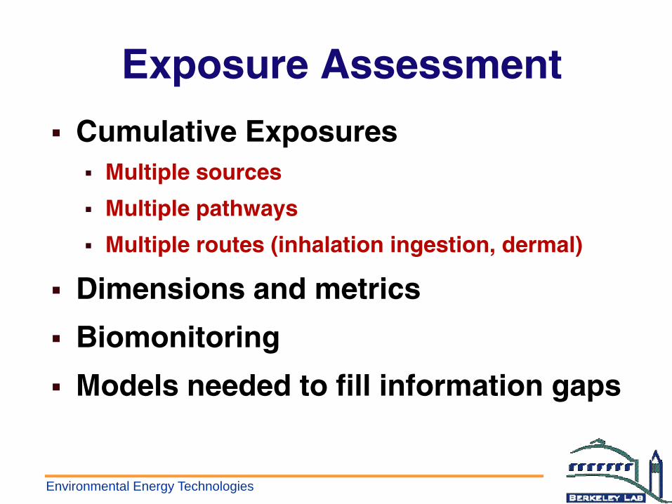
Exposure Assessment

Cumulative ExposuresMultiple sources

Multiple pathways

Multiple routes (inhalation ingestion, dermal)

Dimensions and metrics

Biomonitoring

Models needed to fill information gaps

Chemical intake depends on release location, transport and fate, and human intake through

competing exposure pathways

Do

se

Lifetime average

Do

se

Time (days)

Contact rate

Do

se

Acute exposure event

FoodOutdoor Agricultural

Indoor Water

Dermal, Ingestion, Inhalation

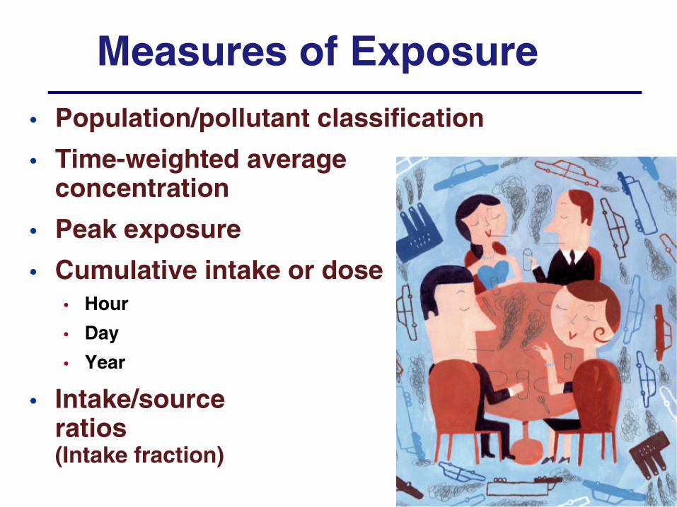
Measures of Exposure

• Population/pollutant classification

• Time-weighted average concentration

• Peak exposure

• Cumulative intake or dose• Hour

• Day

• Year

• Intake/source ratios(Intake fraction)


Biomarkers/Biomonitoring

• BiomarkersSusceptibilityExposure Effect

• Biological mediaBreath SalivaUrine BloodOther--lipid samples, biopsies


Models Fill Information Gaps

Multimedia Mass-Balance Models

Multi-pathway exposure models

Example showing the integration of models and biomarkers

Multimedia Mass Balance Models

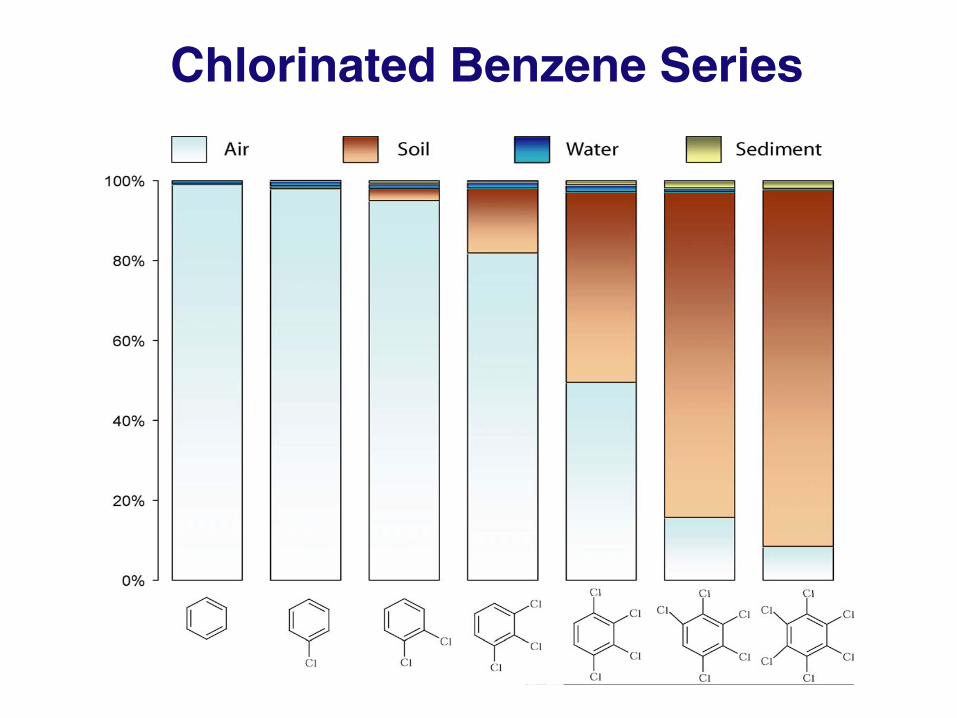
Chlorinated Benzene Series

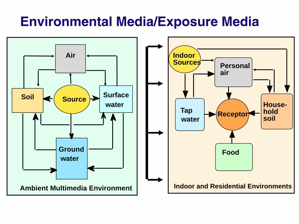
Environmental Media/Exposure Media

IndoorSources

Tapwater

Food

Personalair

House-hold soil

Indoor and Residential Environments

Air

Soil Surface water

Ground water

Source

Ambient Multimedia Environment

Receptor

Organophosphate Pesticide Use

The Salinas Valley is a region of intense pesticide use

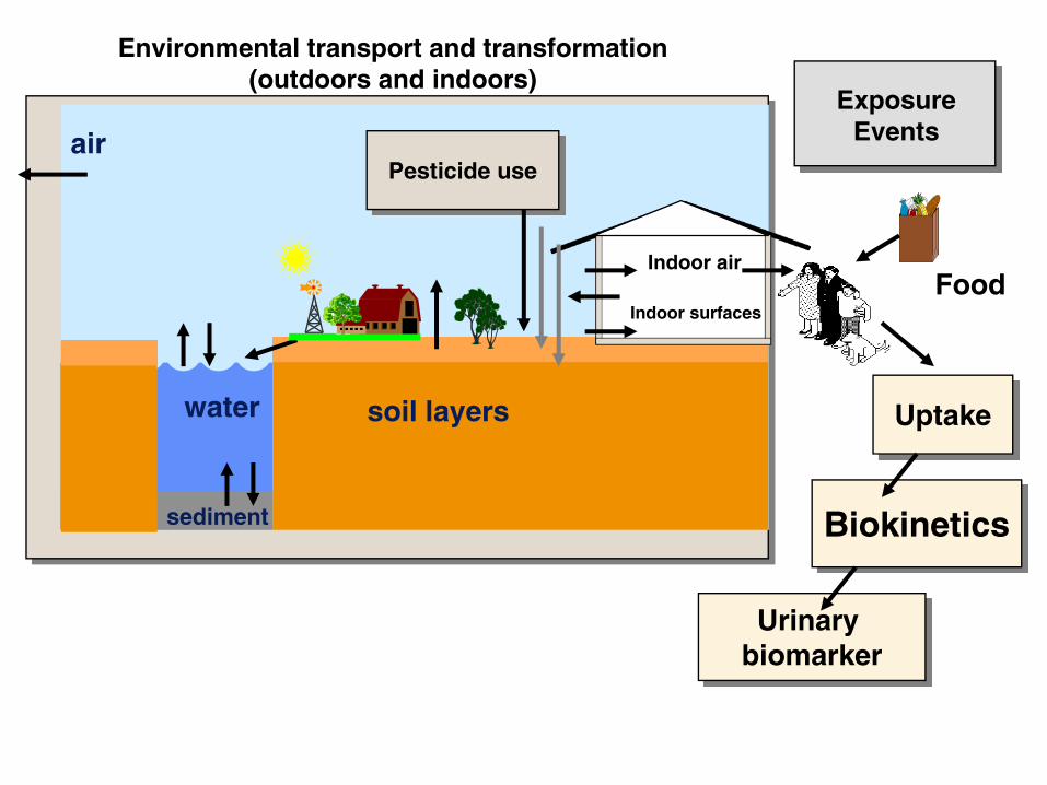
Uptake

Biokinetics

air

water soil layers

sediment

Exposure Events

Pesticide use

Indoor air

Indoor surfaces

Urinary biomarker

Environmental transport and transformation (outdoors and indoors)

Food

Confronting Exposure Potential

• Persistence

• Proximity

• Mobility

Overall Persistence

Chemical inventory or concentration

Sources

Flow from other compartments

Flow to other compartments

Transport out of the landscape

Transformation and decay

Gains LossesCompartment

Transformation and decay

Inventory (mol) = Gains − Losses (mol/d)

Pov(d) = Inventory (mol)Re action Losses(mol/d)

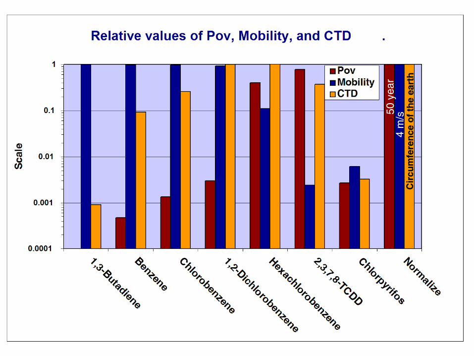
Long-Range Transport Potentialand Mobility

Characteristic travel distance (CTD)

CTD = u/keffective

u = long-term average wind speed

keffective = effective chemical decay rate

Air cell at velocity uN1k1

N1T12

N2T21N2k2

Mobility = Effective Velocity

Depends on wind velocity & “stickiness

Linking Populations to the “Reach” and Proximity of Specific Pollutant Emissions


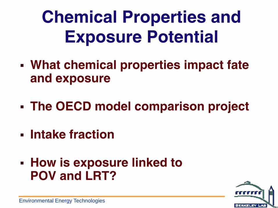
Chemical Properties and Exposure Potential

What chemical properties impact fate and exposure

The OECD model comparison project

Intake fraction

How is exposure linked to POV and LRT?


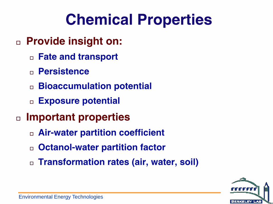
Chemical PropertiesProvide insight on:

Fate and transport

Persistence

Bioaccumulation potential

Exposure potential

Important propertiesAir-water partition coefficient

Octanol-water partition factor

Transformation rates (air, water, soil)

Example References

Chemical Properties and Partitioning

OECD Model Comparison

Response surface applied to 9 Models

Here is an example of oneoutcome mapped against four input parameters over their full range of variation


The Intake Fraction (iF)

= Population IntakeTotal Emissions

=

Ci(t) ⋅ Ini(t)( )i=1

P∑

⎛

⎝ ⎜

⎞

⎠ ⎟ dt

T1

∞∫

E(t) dtT1

T2∫

Ci = Concentration (g/m3)

Ini = Intake rate (m3/person-day),

for example breathing rate

P = Population (persons)

E = Emission rate (g/day)

Intake Fraction Example

Rate of Intake:IR = Ca x B

Steady State Concentration in Air:

Ca = E/V

Loss Rate (Ventilation):Loss = Ca x V

Intake FractioniF = Intake / Emission

iF = (Ca x B) / EiF = B/V

B m3/h

E mol/h

V m3/h

Benzene in the California South Coast Air Basin


Water

Air

Deep soil

Gases Particles

gas

solid liquid

rootingzone

surface soil

Sediment

CalTOXRegional exchange of pollutants among air, soil, water, vegetation etc.

Presenter

Presentation Notes

The purpose of this viewgraph is to help make clear the distinction between air-quality models and multimedia models. Air quality models �address the transport of pollutants moving in air masses - LRT has been well studied for chemicals that reside primarily in the gas phase (i.e., NOx, SOx, CO2 and ozone). These models often have relatively high spatial and temporal resolution and address complex (and often heterogeneous reactions in air. The interactions and soil, water, and vegetation surfaces are handled as simple boundary conditions. But multimedia models �address the regional exchange of pollutants among air, soil, water, vegetation etc. and how this relates to impacts. In contrast to air-quality models these models address the complexity of exchange among air, soil, and water; have complex boundary conditions, but very little spatial and temporal resolution. For many persistent pollutants, environmental transport is controlled in part by the partitioning among and competing degradation rates in various environmental compartments. A multimedia model produces a calculated travel distance for TCDD, a ubiquitous dioxin congener, one order of magnitude greater than an air-dispersion model . Observations of TCDD levels in soil, vegetation, and sediments are consistent with the predictions of the multimedia model. This is because TCDD is rapidly transferred to soil and vegetation and degraded on the surfaces of vegetation. The LRT and impact of multimedia pollutants remains poorly understood. For example, certain combustion by-products (70 dioxins and furans, many PAH's, mercury, and cadmium) may be released to the air but human exposure is primarily through ingestion of food, not inhalation.

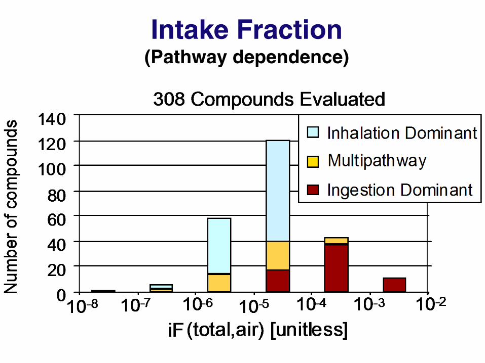
Intake Fraction(Pathway dependence)

Intake Fraction 308 Chemicals


Ranking ToolsExposure depends strongly on:

PersistenceThe longer it lasts the more likely is human intake

CTD is dependent on persistence

Proximity (chemical dependent)CTD defines proximity

MobilityMobility of the pollutant

Mobility of the population

To explore this we use models (CalTOX)

Characteristic Time of Intake (CTI)

Steady State Concentration in Air:

Ca = E/VRate of Intake:

IR = Ca x BVentilation Rate Loss:

VR = Ca x V

iF = (Ca x B) / (Ca x V)

= B / V

Intake fraction can be viewed as a competition between the rate of chemical uptake by the population (B) and the rate of clearance from the environment (V)

B m3/h

E mol/h

V m3/h


The relationship betweeniF and Pov:

iF =

PovCTI

Where, at steady state,

M = Inventory of chemical in the environmental system

Pov = M / emission rate

CTI = M / population intake rate

CTI for Regional Multimedia Multipathway Exposures (CalTOX)

air

water soil layers

sediment

emissions

Exposure mediaPopulation intake

Environmental media

AirFoodWaterSoil

CTI for 315 Chemicals Using CalTOX Applied to North American Region

with iF versus Tov (Persistence)

Emissions to Air Emissions to Water

iF Based on Canadian Emissions Inventories, Environmental Concentrations and Food Basket Surveys

[CEPA PSL1 reports (20010]

Pov (=Tov) estimated from chemical-specific degradation rates in a generic environment


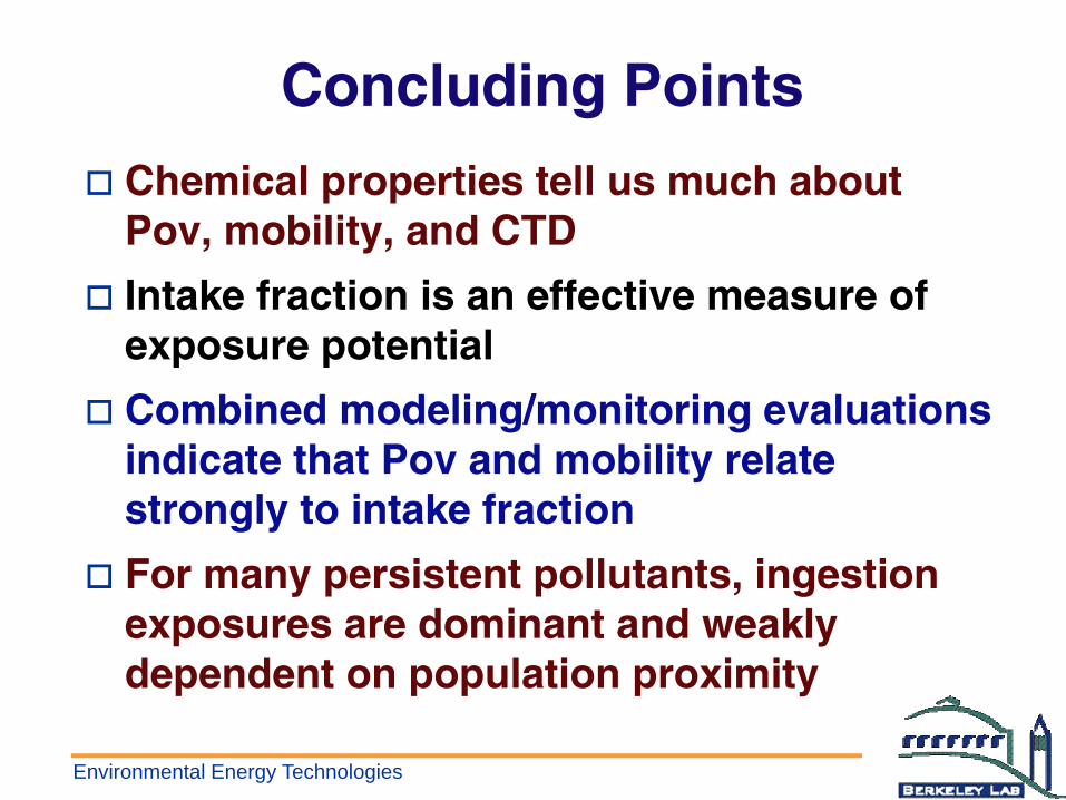
Concluding Points

Chemical properties tell us much about Pov, mobility, and CTD

Intake fraction is an effective measure of exposure potential

Combined modeling/monitoring evaluations indicate that Pov and mobility relate strongly to intake fraction

For many persistent pollutants, ingestion exposures are dominant and weakly dependent on population proximity

tools for predicting exposure potential - oehha · pdf fileenvironmental energy technologies...

Documents