6 -1

Topic 4 - Pulp Suspensions

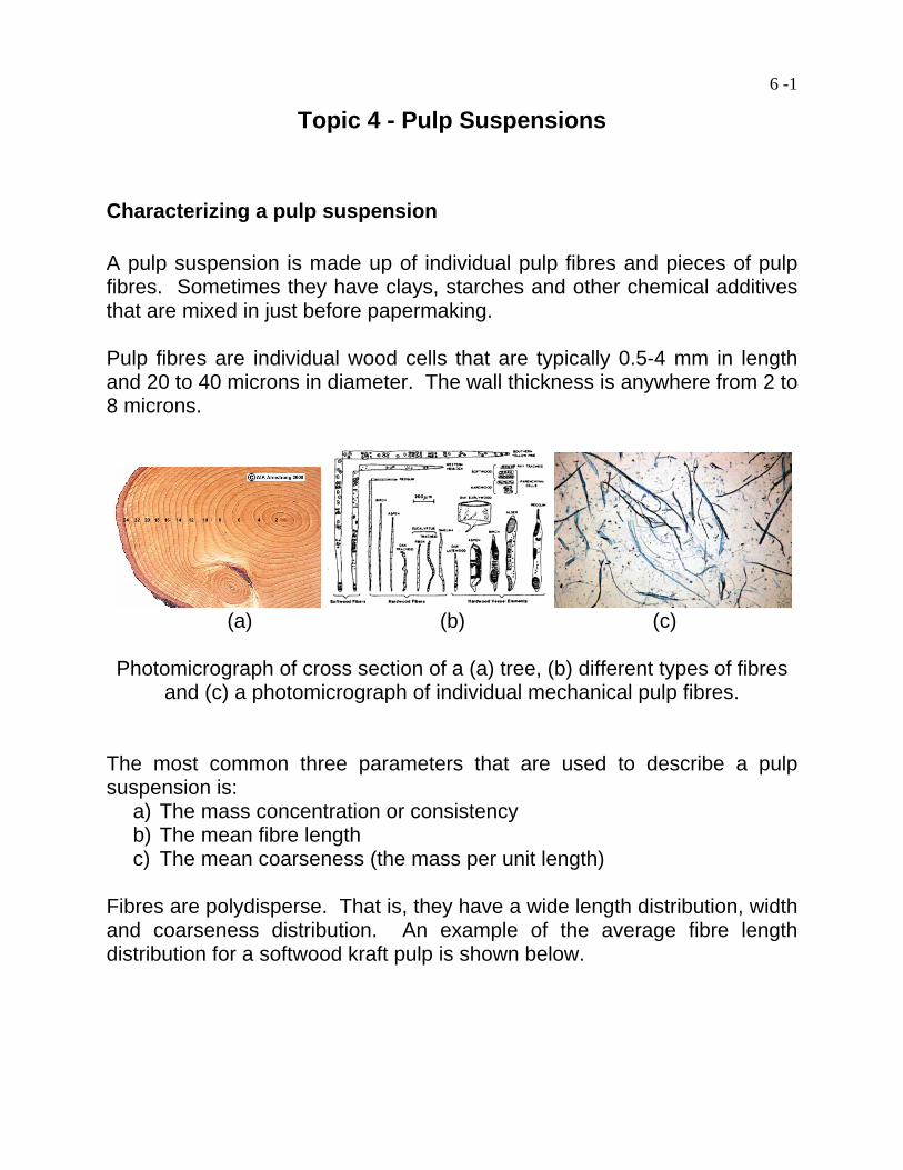
Characterizing a pulp suspension A pulp suspension is made up of individual pulp fibres and pieces of pulp fibres. Sometimes they have clays, starches and other chemical additives that are mixed in just before papermaking. Pulp fibres are individual wood cells that are typically 0.5-4 mm in length and 20 to 40 microns in diameter. The wall thickness is anywhere from 2 to 8 microns.

(a) (b) (c)

Photomicrograph of cross section of a (a) tree, (b) different types of fibres

and (c) a photomicrograph of individual mechanical pulp fibres. The most common three parameters that are used to describe a pulp suspension is:

a) The mass concentration or consistency b) The mean fibre length c) The mean coarseness (the mass per unit length)

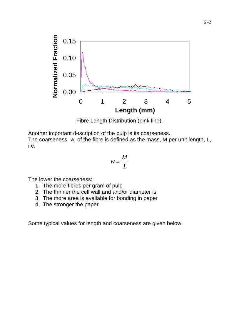
Fibres are polydisperse. That is, they have a wide length distribution, width and coarseness distribution. An example of the average fibre length distribution for a softwood kraft pulp is shown below.

6 -2

0.00

0.05

0.10

0.15

0 1 2 3 4 5Length (mm)

Nor

mal

ized

Fra

ctio

n

Fibre Length Distribution (pink line).

Another important description of the pulp is its coarseness. The coarseness, w, of the fibre is defined as the mass, M per unit length, L, i.e,

MwL

=

The lower the coarseness:

1. The more fibres per gram of pulp 2. The thinner the cell wall and and/or diameter is. 3. The more area is available for bonding in paper 4. The stronger the paper.

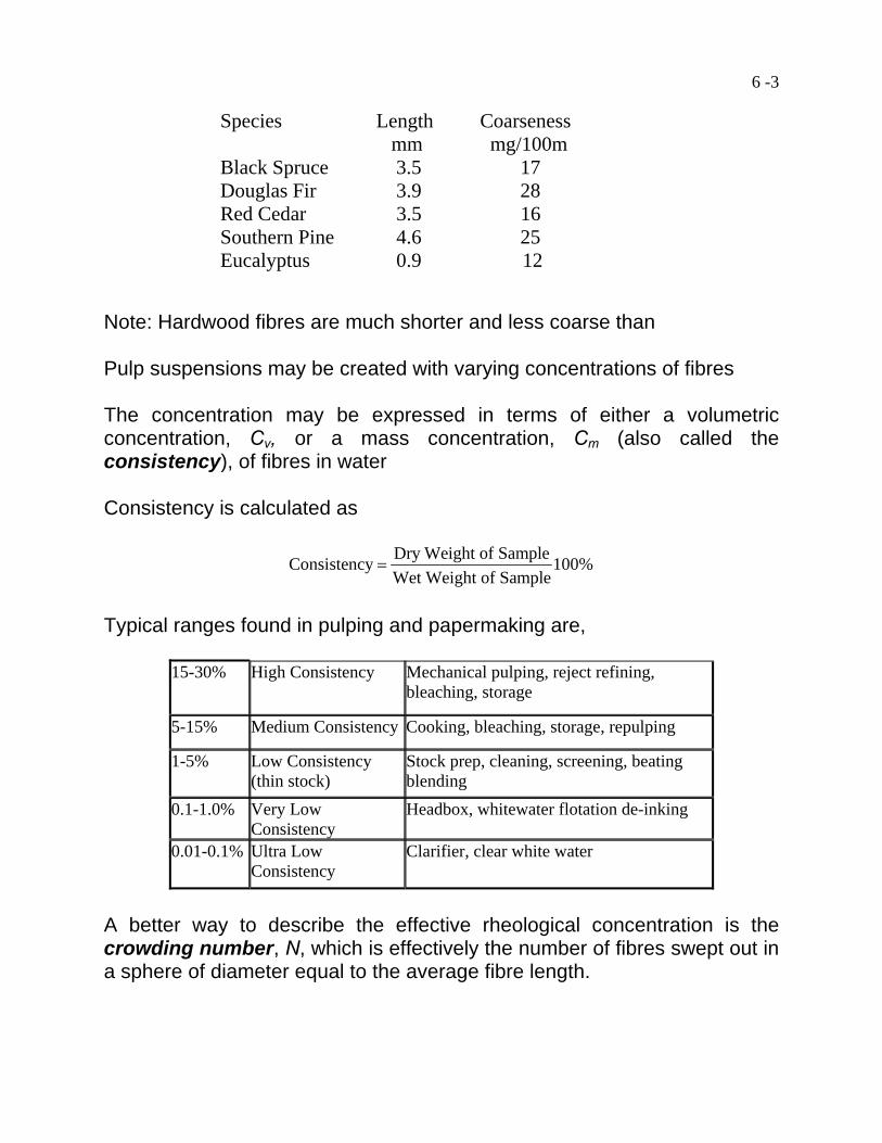
Some typical values for length and coarseness are given below:

6 -3

Note: Hardwood fibres are much shorter and less coarse than Pulp suspensions may be created with varying concentrations of fibres The concentration may be expressed in terms of either a volumetric concentration, Cv, or a mass concentration, Cm (also called the consistency), of fibres in water Consistency is calculated as Dry Weight of SampleConsistency 100%

Wet Weight of Sample=

Typical ranges found in pulping and papermaking are,

15-30% High Consistency Mechanical pulping, reject refining, bleaching, storage

5-15% Medium Consistency Cooking, bleaching, storage, repulping

1-5% Low Consistency (thin stock)

Stock prep, cleaning, screening, beating blending

0.1-1.0% Very Low Consistency

Headbox, whitewater flotation de-inking

0.01-0.1% Ultra Low Consistency

Clarifier, clear white water

A better way to describe the effective rheological concentration is the crowding number, N, which is effectively the number of fibres swept out in a sphere of diameter equal to the average fibre length.

Species Length Coarseness mm mg/100m Black Spruce 3.5 17 Douglas Fir 3.9 28 Red Cedar 3.5 16 Southern Pine 4.6 25 Eucalyptus 0.9 12

6 -4

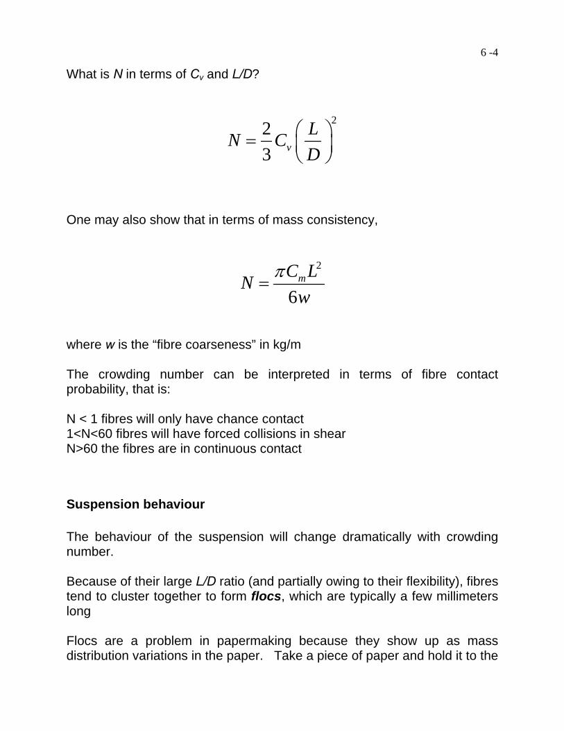
What is N in terms of Cv and L/D?

223 v

LN CD

⎛ ⎞= ⎜ ⎟⎝ ⎠

One may also show that in terms of mass consistency,

2

6mC LNw

π=

where w is the “fibre coarseness” in kg/m The crowding number can be interpreted in terms of fibre contact probability, that is: N < 1 fibres will only have chance contact 1<N<60 fibres will have forced collisions in shear N>60 the fibres are in continuous contact

Suspension behaviour The behaviour of the suspension will change dramatically with crowding number. Because of their large L/D ratio (and partially owing to their flexibility), fibres tend to cluster together to form flocs, which are typically a few millimeters long Flocs are a problem in papermaking because they show up as mass distribution variations in the paper. Take a piece of paper and hold it to the

6 -5

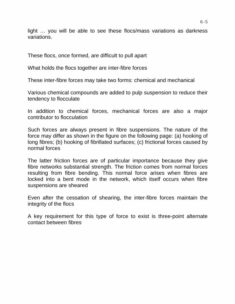
light … you will be able to see these flocs/mass variations as darkness variations. These flocs, once formed, are difficult to pull apart What holds the flocs together are inter-fibre forces These inter-fibre forces may take two forms: chemical and mechanical Various chemical compounds are added to pulp suspension to reduce their tendency to flocculate In addition to chemical forces, mechanical forces are also a major contributor to flocculation Such forces are always present in fibre suspensions. The nature of the force may differ as shown in the figure on the following page: (a) hooking of long fibres; (b) hooking of fibrillated surfaces; (c) frictional forces caused by normal forces The latter friction forces are of particular importance because they give fibre networks substantial strength. The friction comes from normal forces resulting from fibre bending. This normal force arises when fibres are locked into a bent mode in the network, which itself occurs when fibre suspensions are sheared Even after the cessation of shearing, the inter-fibre forces maintain the integrity of the flocs A key requirement for this type of force to exist is three-point alternate contact between fibres

6 -6

6 -7

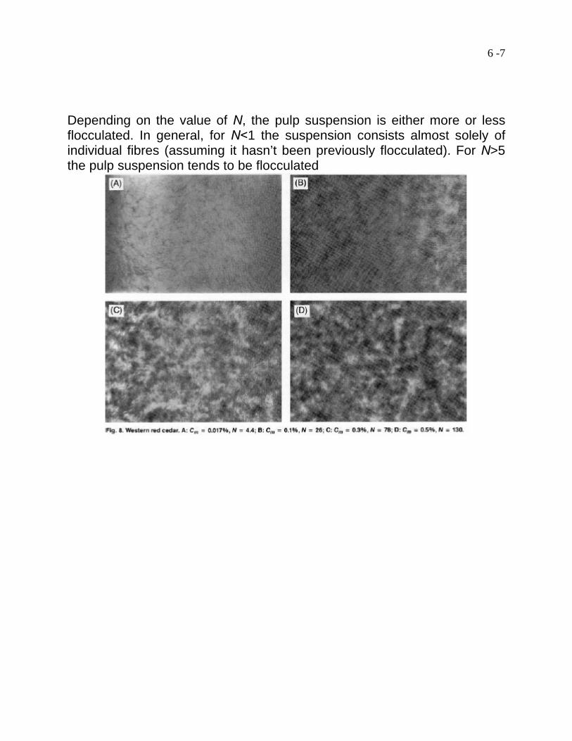
Depending on the value of N, the pulp suspension is either more or less flocculated. In general, for N<1 the suspension consists almost solely of individual fibres (assuming it hasn’t been previously flocculated). For N>5 the pulp suspension tends to be flocculated

6 -8

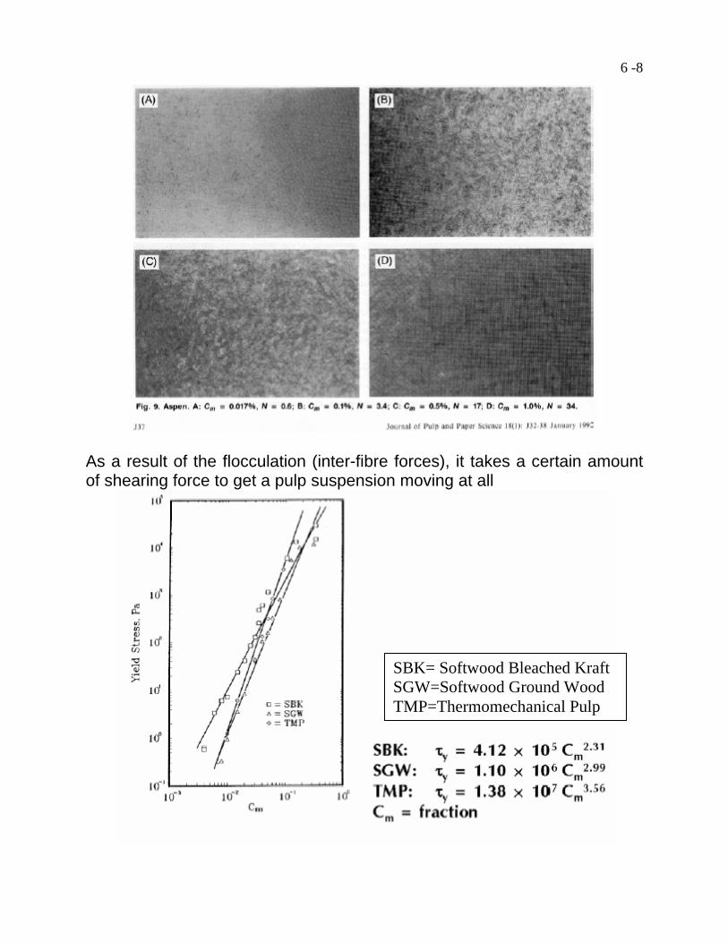
As a result of the flocculation (inter-fibre forces), it takes a certain amount of shearing force to get a pulp suspension moving at all

SBK= Softwood Bleached Kraft SGW=Softwood Ground Wood TMP=Thermomechanical Pulp

6 -9

In other words, the pulp suspension acts like a non-Newtonian fluid with a finite yield stress (like a Bingham plastic). This yield stress is a function of the consistency and the type of pulp tested Pulp suspension can only flow once this shear stress is exceeded in the suspension Once the suspension starts to flow, the flow can be in the form of flocs slipping past flocs, or individual fibres slipping past one another The shear stress required to get pulp suspension to flow is generally higher than would be attained in laminar flow, so industrially it is only sensible to speak of turbulent pulp flow Shear levels in turbulent flow of fibre suspensions are very difficult to quantify. One of the most useful quantitative parameters we have for accomplishing this is the power dissipation per unit volume, εF This is a useful parameter because, as we know from our discussion of the Kolmogorov scale, turbulent energy in a fluid cascades down into smaller eddies and ultimately dissipates as heat The level of energy dissipation directly reflects the turbulent shear of the small scale eddies. This shear causes fibre level fluidization Several workers have measured power dissipation per unit volume required to cause fibre suspension fluidization This measurement is not precise because strong gradients of shear exist in any practical vessel used to measure fluidization, and definitions of fluidization have been imprecise i.e. floc level or fibre level. Some values are given on the following page

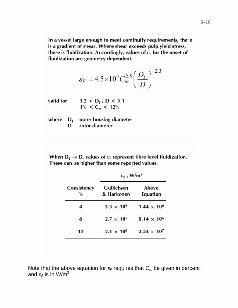
6 -10

Note that the above equation for εF requires that Cm be given in percent and εF is in W/m3

6 -11

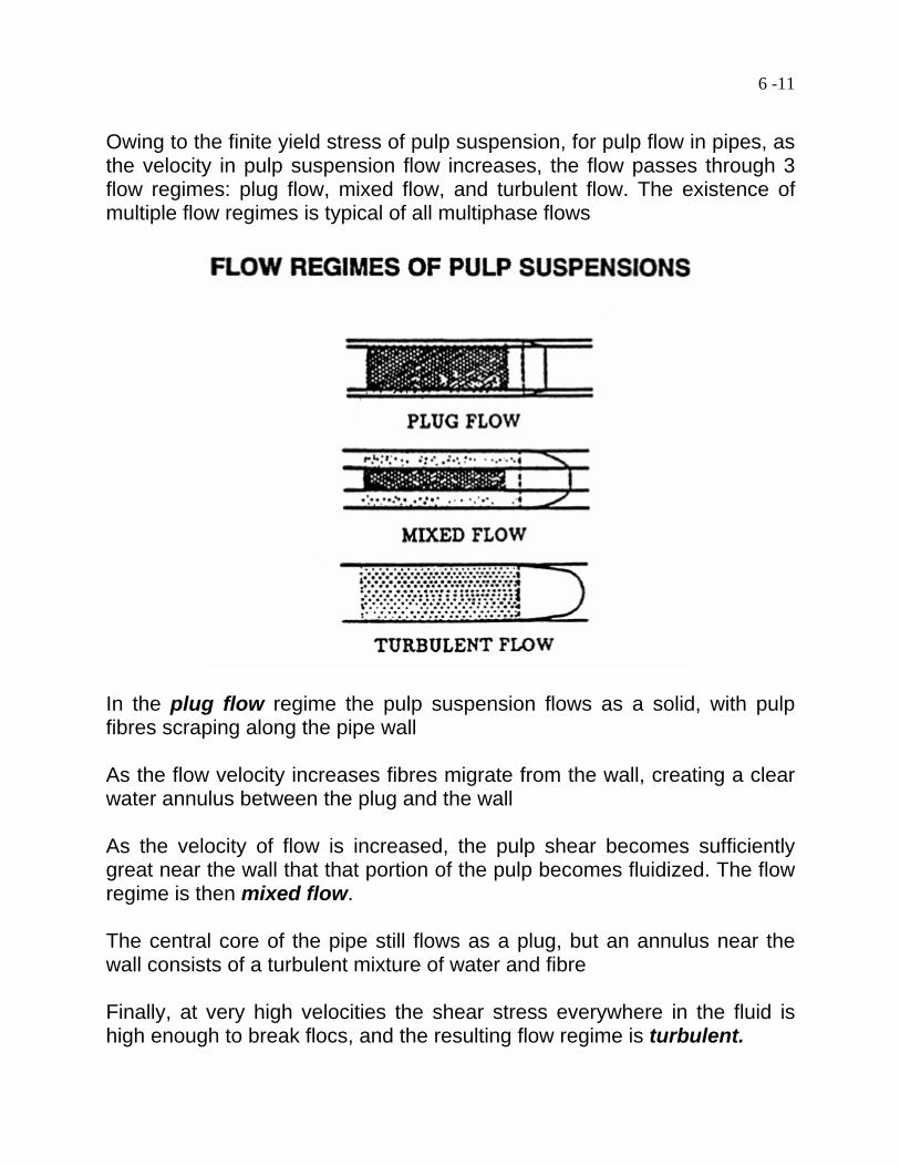
Owing to the finite yield stress of pulp suspension, for pulp flow in pipes, as the velocity in pulp suspension flow increases, the flow passes through 3 flow regimes: plug flow, mixed flow, and turbulent flow. The existence of multiple flow regimes is typical of all multiphase flows

In the plug flow regime the pulp suspension flows as a solid, with pulp fibres scraping along the pipe wall As the flow velocity increases fibres migrate from the wall, creating a clear water annulus between the plug and the wall As the velocity of flow is increased, the pulp shear becomes sufficiently great near the wall that that portion of the pulp becomes fluidized. The flow regime is then mixed flow. The central core of the pipe still flows as a plug, but an annulus near the wall consists of a turbulent mixture of water and fibre Finally, at very high velocities the shear stress everywhere in the fluid is high enough to break flocs, and the resulting flow regime is turbulent.

6 -12

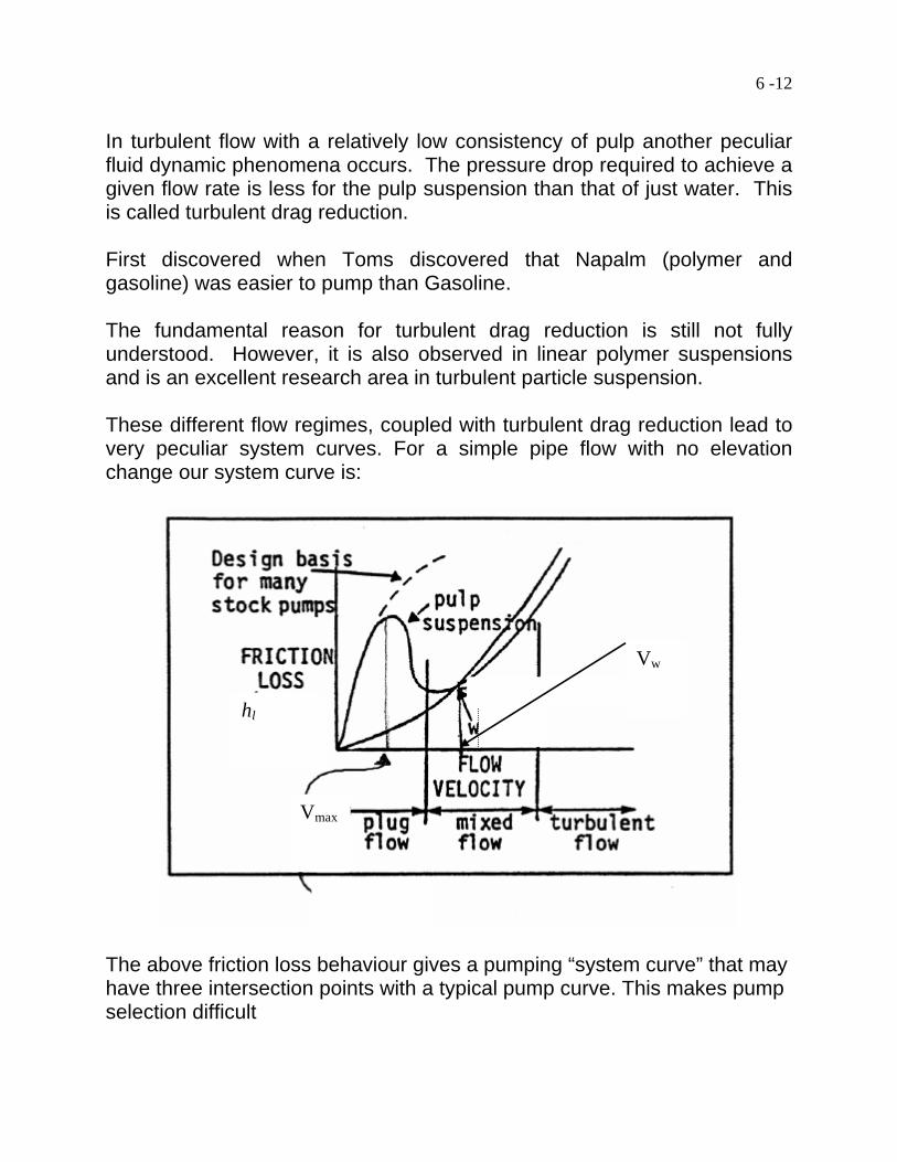
In turbulent flow with a relatively low consistency of pulp another peculiar fluid dynamic phenomena occurs. The pressure drop required to achieve a given flow rate is less for the pulp suspension than that of just water. This is called turbulent drag reduction. First discovered when Toms discovered that Napalm (polymer and gasoline) was easier to pump than Gasoline. The fundamental reason for turbulent drag reduction is still not fully understood. However, it is also observed in linear polymer suspensions and is an excellent research area in turbulent particle suspension. These different flow regimes, coupled with turbulent drag reduction lead to very peculiar system curves. For a simple pipe flow with no elevation change our system curve is:

The above friction loss behaviour gives a pumping “system curve” that may have three intersection points with a typical pump curve. This makes pump selection difficult

Vmax

hl

Vw

6 -13

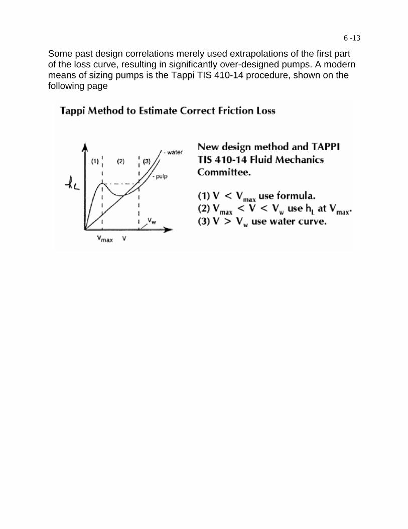
Some past design correlations merely used extrapolations of the first part of the loss curve, resulting in significantly over-designed pumps. A modern means of sizing pumps is the Tappi TIS 410-14 procedure, shown on the following page

6 -14

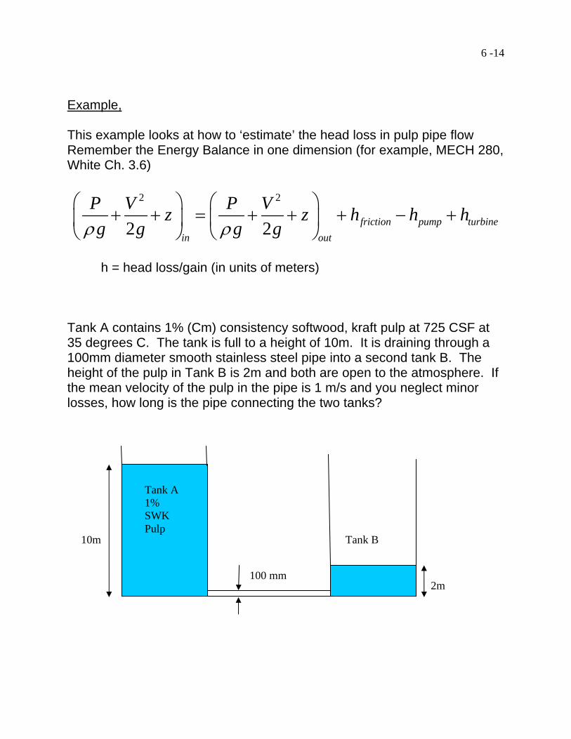
Example, This example looks at how to ‘estimate’ the head loss in pulp pipe flow Remember the Energy Balance in one dimension (for example, MECH 280, White Ch. 3.6)

2 2

2 2 friction pump turbinein out

P V P Vz z h h hg g g gρ ρ

⎛ ⎞ ⎛ ⎞+ + = + + + − +⎜ ⎟ ⎜ ⎟

⎝ ⎠ ⎝ ⎠

h = head loss/gain (in units of meters) Tank A contains 1% (Cm) consistency softwood, kraft pulp at 725 CSF at 35 degrees C. The tank is full to a height of 10m. It is draining through a 100mm diameter smooth stainless steel pipe into a second tank B. The height of the pulp in Tank B is 2m and both are open to the atmosphere. If the mean velocity of the pulp in the pipe is 1 m/s and you neglect minor losses, how long is the pipe connecting the two tanks?

10m

2m 100 mm

Tank A 1% SWK Pulp

Tank B