topic 8 hypothesis testing mathematics & statistics statistics
TRANSCRIPT
Topic 8
Hypothesis Testing
Mathematics & Statistics Statistics

Topic Goals
After completing this topic, you should be able to:
Formulate null and alternative hypotheses for applications involving
a population mean from a normal distribution a population proportion (large samples)
Formulate a decision rule for testing a hypothesis Know how to use the critical value and p-value
approaches to test the null hypothesis (for both mean and proportion problems)
Know what Type I and Type II errors are Assess the power of a test
What is a Hypothesis?
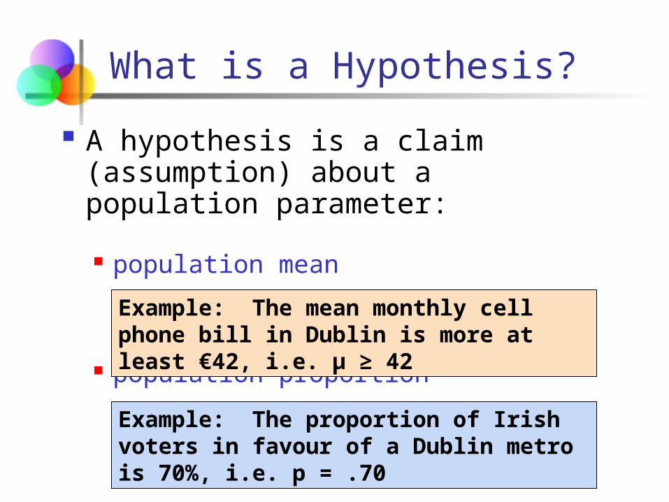
A hypothesis is a claim (assumption) about a population parameter:
population mean
population proportion
Example: The mean monthly cell phone bill in Dublin is more at least €42, i.e. μ ≥ 42
Example: The proportion of Irish voters in favour of a Dublin metro is 70%, i.e. p = .70
Hypothesis testing Procedure
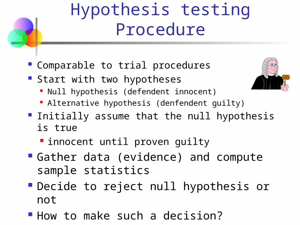
Comparable to trial procedures Start with two hypotheses
Null hypothesis (defendent innocent) Alternative hypothesis (denfendent guilty)
Initially assume that the null hypothesis is true innocent until proven guilty
Gather data (evidence) and compute sample statistics
Decide to reject null hypothesis or not How to make such a decision?
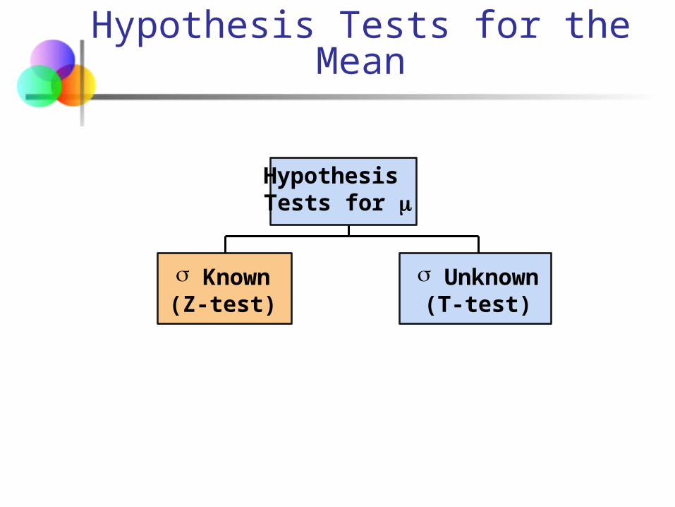
Hypothesis Tests for the Mean
Known(Z-test)
Unknown(T-test)
Hypothesis Tests for
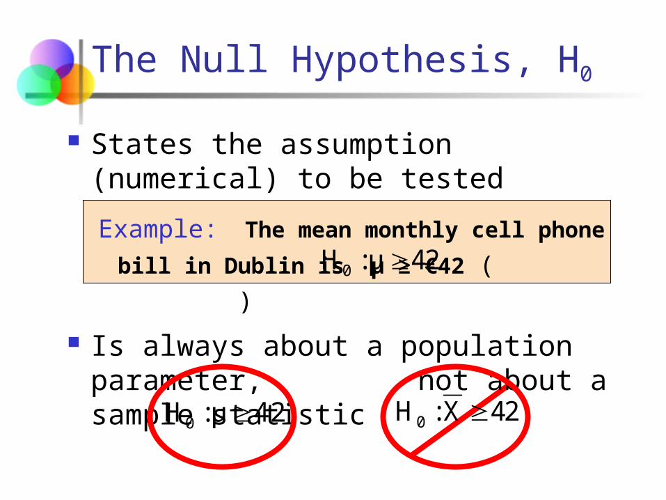
The Null Hypothesis, H0
States the assumption (numerical) to be tested
Example: The mean monthly cell phone bill in
Dublin is μ ≥ €42 ( )
Is always about a population parameter, not about a sample statistic
24μ:H0
42μ:H0 24X:H0
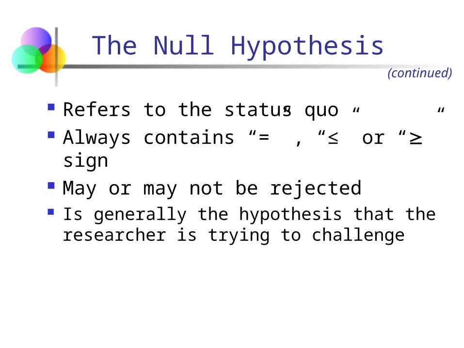
The Null Hypothesis
Refers to the status quo Always contains “=” , “≤” or “” sign May or may not be rejected Is generally the hypothesis that the researcher
is trying to challenge
(continued)
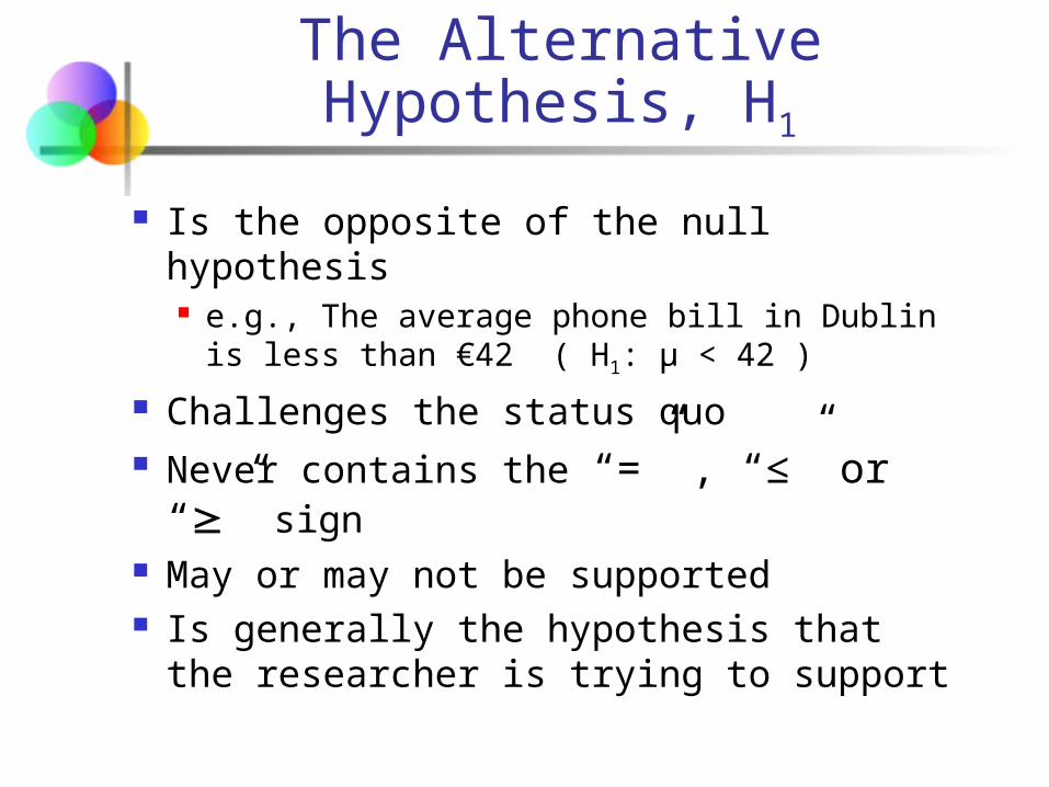
The Alternative Hypothesis, H1
Is the opposite of the null hypothesis e.g., The average phone bill in Dublin is less
than €42 ( H1: μ < 42 )
Challenges the status quo Never contains the “=” , “≤” or “” sign May or may not be supported Is generally the hypothesis that the
researcher is trying to support
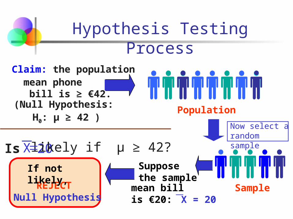
Population
Claim: the populationmean phone bill is ≥ €42.(Null Hypothesis:
REJECT
Supposethe samplemean bill is €20: X = 20
SampleNull Hypothesis
20 likely if μ ≥ 42?Is
Hypothesis Testing Process
If not likely,
Now select a random sample
H0: μ ≥ 42 )
X
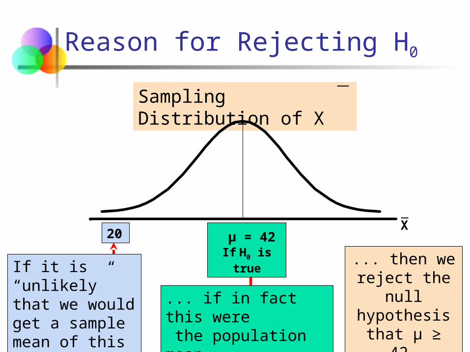
Sampling Distribution of X
μ = 42If H0 is true
If it is “unlikely” that we would get a sample mean of this value ...
... then we reject the null
hypothesis that μ ≥ 42.
Reason for Rejecting H0
20
... if in fact this were the population mean…
X
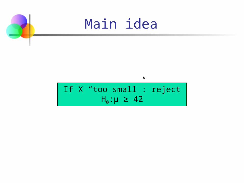
Main idea
If X “too small”: reject H0:μ ≥ 42
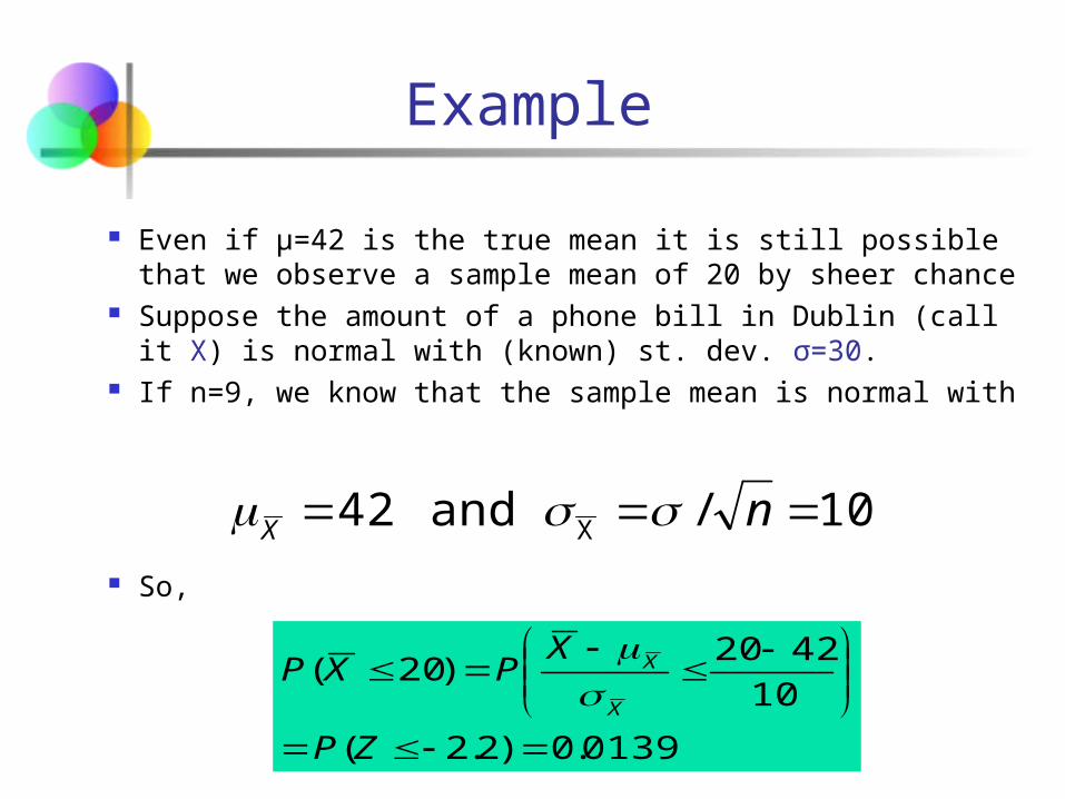
Example
Even if μ=42 is the true mean it is still possible that we observe a sample mean of 20 by sheer chance
Suppose the amount of a phone bill in Dublin (call it X) is normal with (known) st. dev. σ=30.
If n=9, we know that the sample mean is normal with
So,
10/and42 X nX
0139.0)2.2(
10
4220)20(
ZP
XPXP
X
X
Example
So, if we find a sample mean of 20 and if the population mean is 42...
...we have observed an event that occurs with probability .0139.
Do we deem this “unlikely”? Below what probability will we call an event
“unlikely”? This threshold probability is chosen by the
researcher and is called the....
(continued)
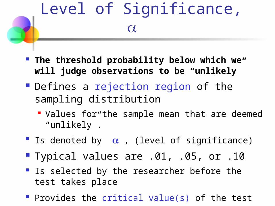
Level of Significance,
The threshold probability below which we will judge observations to be “unlikely”
Defines a rejection region of the sampling distribution Values for the sample mean that are deemed
“unlikely”.
Is denoted by , (level of significance)
Typical values are .01, .05, or .10 Is selected by the researcher before the test takes place
Provides the critical value(s) of the test
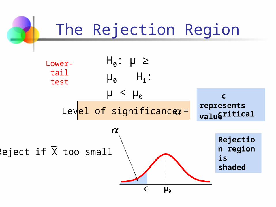
The Rejection Region
H0: μ ≥ μ0
H1: μ < μ0
μ0
c represents critical value
Lower-tail test
Level of significance =
Rejection region is shaded
Reject if X too small
c
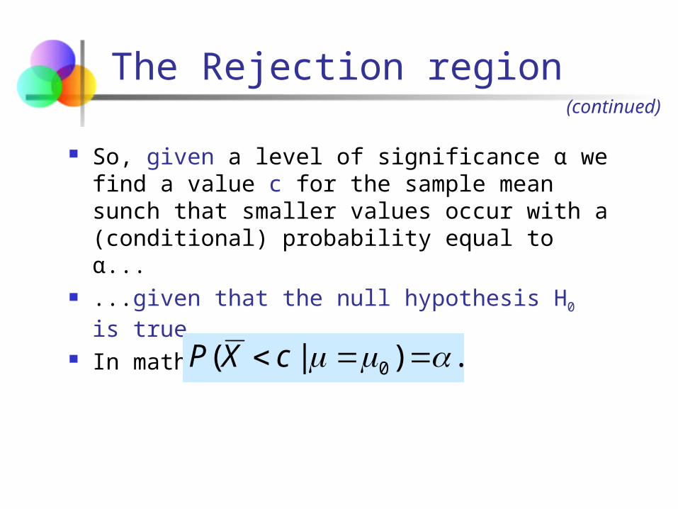
The Rejection region
So, given a level of significance α we find a value c for the sample mean sunch that smaller values occur with a (conditional) probability equal to α...
...given that the null hypothesis H0 is true. In mathematical notation:
(continued)
.)|( 0 cXP
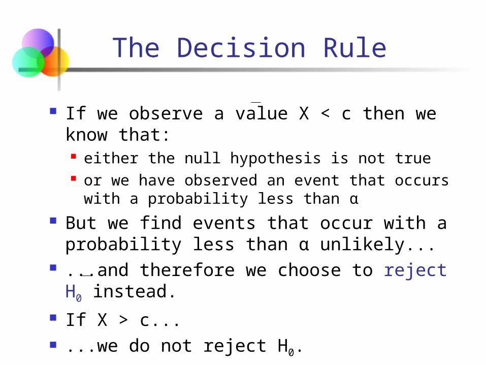
The Decision Rule
If we observe a value X < c then we know that:
either the null hypothesis is not true or we have observed an event that occurs with a
probability less than α But we find events that occur with a probability
less than α unlikely... ...and therefore we choose to reject H0 instead. If X > c... ...we do not reject H0.
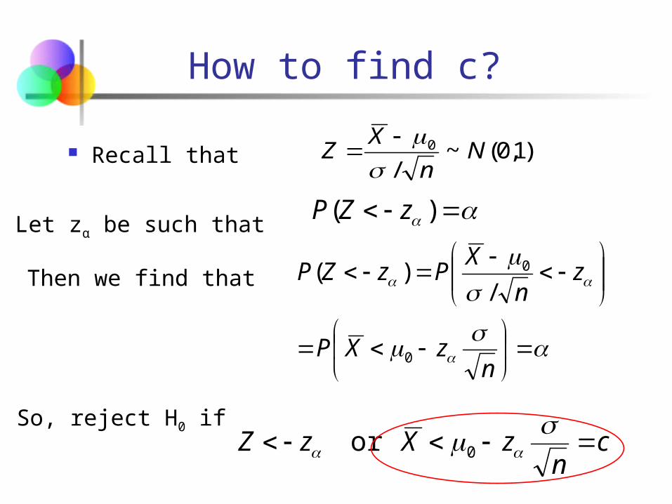
How to find c?
Recall that )1,0(~/
0 Nn
XZ
Let zα be such that )( zZP
Then we find that
nzXP
zn
XPzZP
0
0
/)(
So, reject H0 ifc
nzXzZ
0or
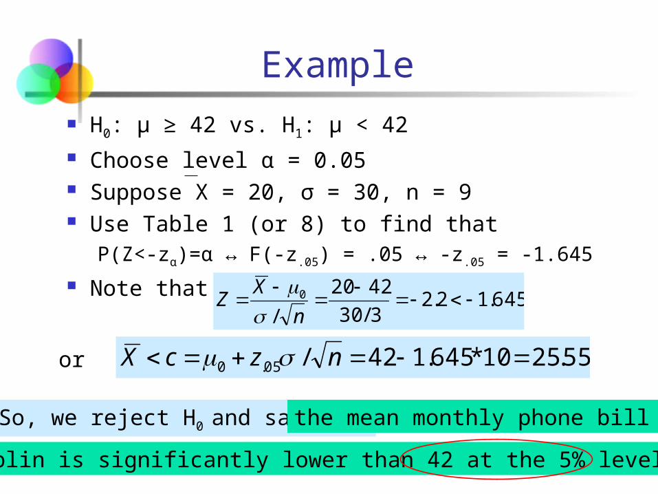
Example
H0: μ ≥ 42 vs. H1: μ < 42 Choose level α = 0.05 Suppose X = 20, σ = 30, n = 9 Use Table 1 (or 8) to find that
P(Z<-zα)=α ↔ F(-z.05) = .05 ↔ -z.05 = -1.645
Note that 645.12.23/30
4220
/0
n
XZ
or 55.2510*645.142/05.0 nzcX
So, we reject H0 and say that the mean monthly phone bill in
Dublin is significantly lower than 42 at the 5% level
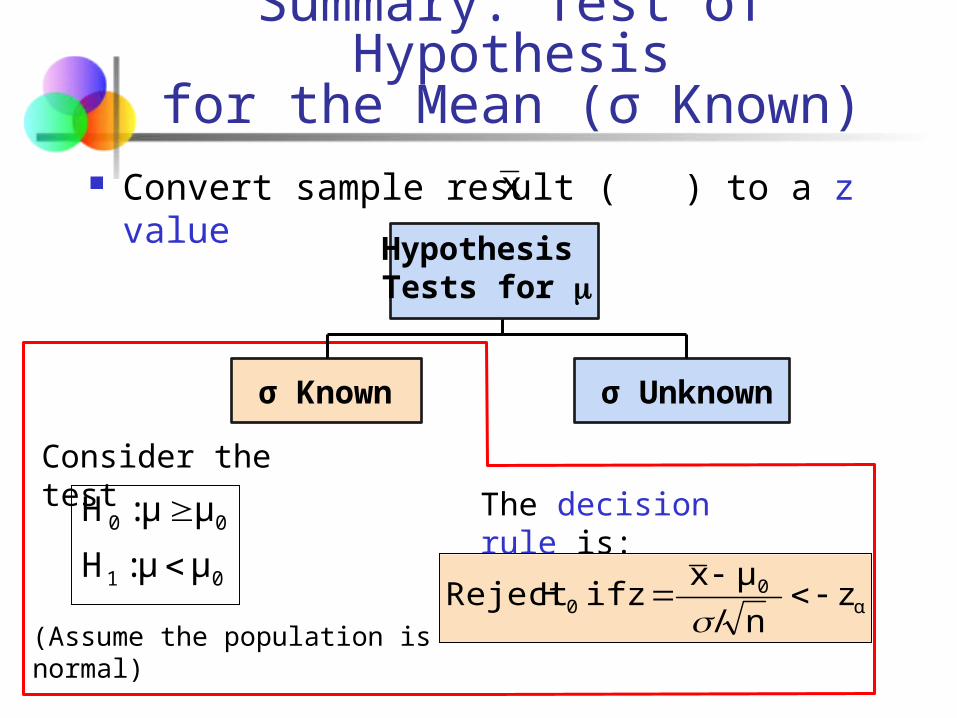
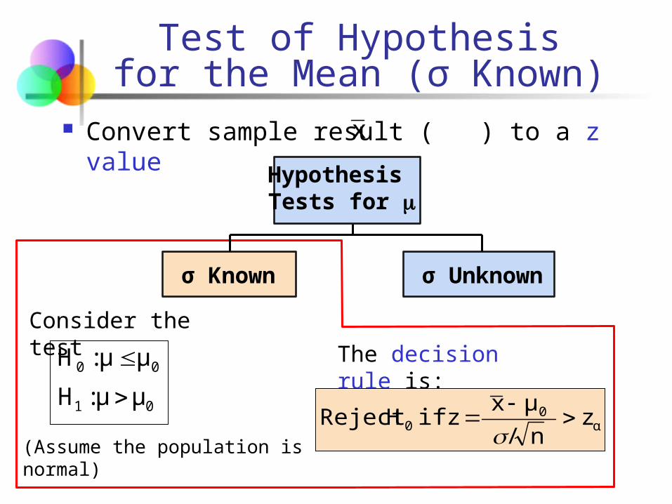
Summary: Test of Hypothesisfor the Mean (σ Known)
Convert sample result ( ) to a z value
The decision rule is:
α0
0 zn/
μxz if HReject
σ Known σ Unknown
Hypothesis Tests for
Consider the test
00 μμ:H
01 μμ:H
(Assume the population is normal)
x
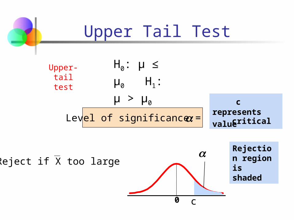
Upper Tail Test
H0: μ ≤ μ0
H1: μ > μ0
0
c represents critical value
Upper-tail test
Level of significance =
Rejection region is shaded
Reject if X too large
c
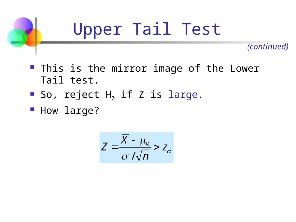
Upper Tail Test
This is the mirror image of the Lower Tail test. So, reject H0 if Z is large. How large?
(continued)
zn
XZ
/0
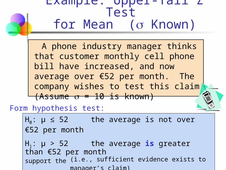
Example: Upper-Tail Z Test for Mean ( Known)
A phone industry manager thinks that customer monthly cell phone bill have increased, and now average over €52 per month. The company wishes to test this claim. (Assume = 10 is known)
H0: μ ≤ 52 the average is not over €52 per month
H1: μ > 52 the average is greater than €52 per month(i.e., sufficient evidence exists to support the manager’s claim)
Form hypothesis test:
Reject H0Do not reject H0
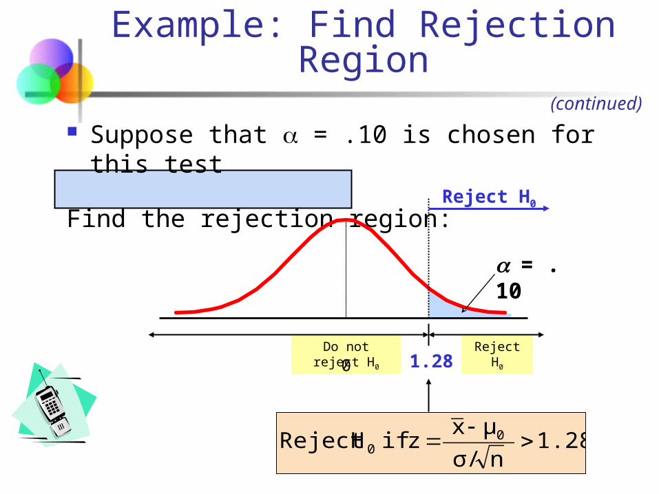
Suppose that = .10 is chosen for this test
Find the rejection region:
= .10
1.280
Reject H0
Example: Find Rejection Region(continued)
1.28nσ/
μxz if H Reject 0
0
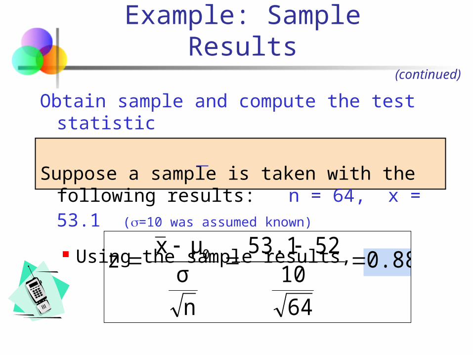
Obtain sample and compute the test statistic
Suppose a sample is taken with the following results: n = 64, x = 53.1 (=10 was assumed known)
Using the sample results,
0.88
64
105253.1
n
σμx
z 0
Example: Sample Results(continued)
Reject H0Do not reject H0
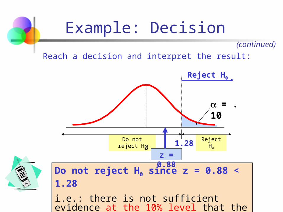
Example: Decision
= .10
1.280
Reject H0
Do not reject H0 since z = 0.88 < 1.28
i.e.: there is not sufficient evidence at the 10% level that the mean bill is over €52
z = 0.88
Reach a decision and interpret the result:(continued)
Test of Hypothesisfor the Mean (σ Known)
Convert sample result ( ) to a z value
The decision rule is:
α0
0 zn/
μxz if HReject
σ Known σ Unknown
Hypothesis Tests for
Consider the test
00 μμ:H
01 μμ:H
(Assume the population is normal)
x
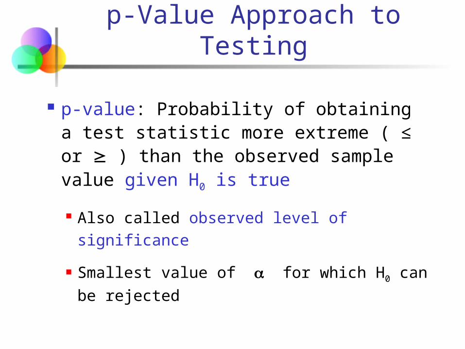
p-Value Approach to Testing
p-value: Probability of obtaining a test statistic more extreme ( ≤ or ) than the observed sample value given H0 is
true
Also called observed level of significance
Smallest value of for which H0 can be
rejected
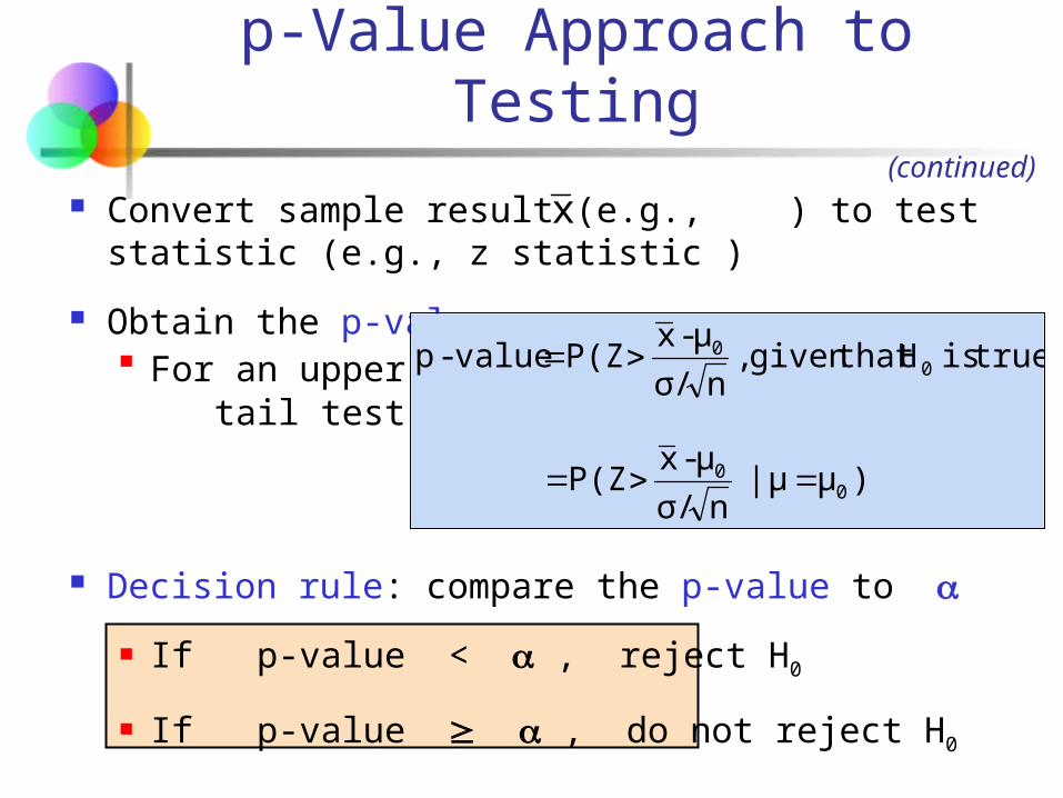
p-Value Approach to Testing
Convert sample result (e.g., ) to test statistic (e.g., z statistic )
Obtain the p-value For an upper
tail test:
Decision rule: compare the p-value to
If p-value < , reject H0
If p-value , do not reject H0
(continued)
x
)μμ | nσ/
μ-x P(Z
true) is H that given , nσ/
μ-x P(Z value-p
00
00

Example: Upper-Tail Z Test for Mean ( Known)
A phone industry manager thinks that customer monthly cell phone bill have increased, and now average over €52 per month. The company wishes to test this claim. (Assume = 10 is known)
H0: μ ≤ 52 the average is not over €52 per month
H1: μ > 52 the average is greater than €52 per month(i.e., sufficient evidence exists to support the manager’s claim)
Form hypothesis test:
Reject H0
= .10
Do not reject H0 1.28
0
Reject H0
Z = .88
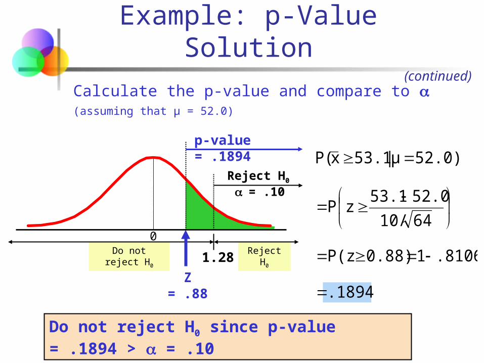
Calculate the p-value and compare to (assuming that μ = 52.0)
(continued)
.1894
.810610.88)P(z
6410/
52.053.1zP
52.0) μ | 53.1xP(
p-value = .1894
Example: p-Value Solution
Do not reject H0 since p-value = .1894 > = .10
Do not reject H0 Reject H0Reject H0
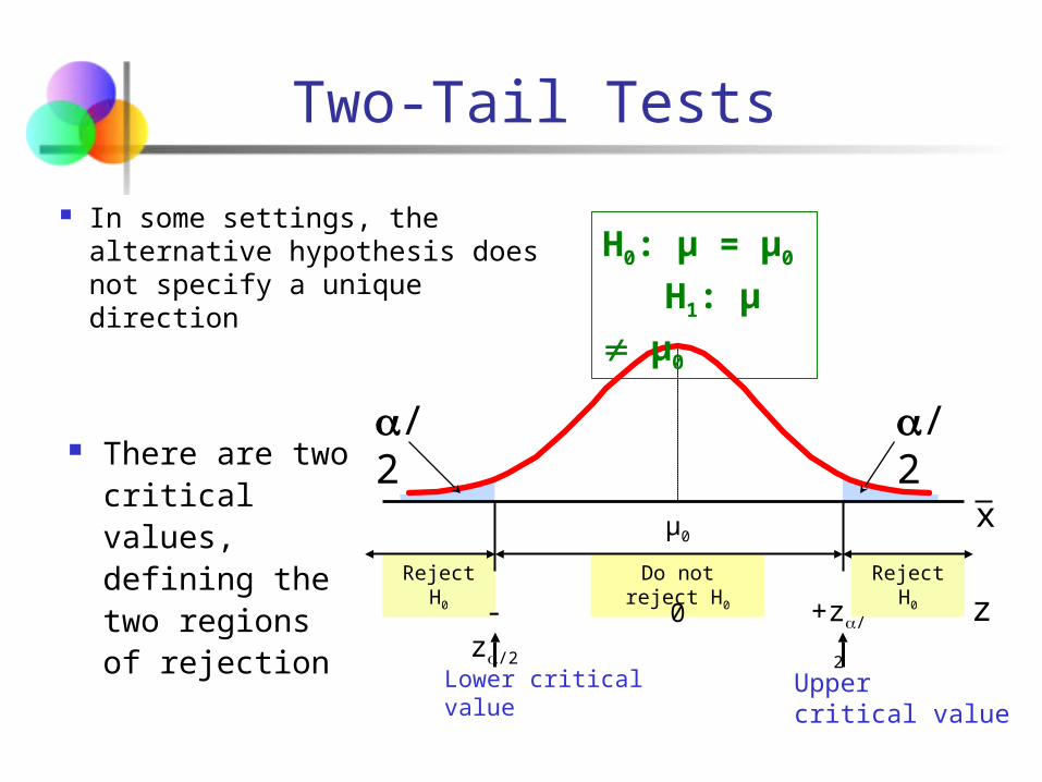
There are two critical values, defining the two regions of rejection
Two-Tail Tests
/2
0
H0: μ = μ0
H1: μ μ0
/2
Lower critical value
Uppercritical value
μ0
z
x
-z/2 +z/2
In some settings, the alternative hypothesis does not specify a unique direction
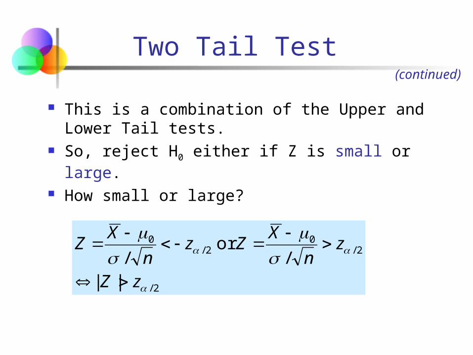
Two Tail Test
This is a combination of the Upper and Lower Tail tests.
So, reject H0 either if Z is small or large. How small or large?
(continued)
2/
2/0
2/0
||/
or/
zZ
zn
XZz
n
XZ
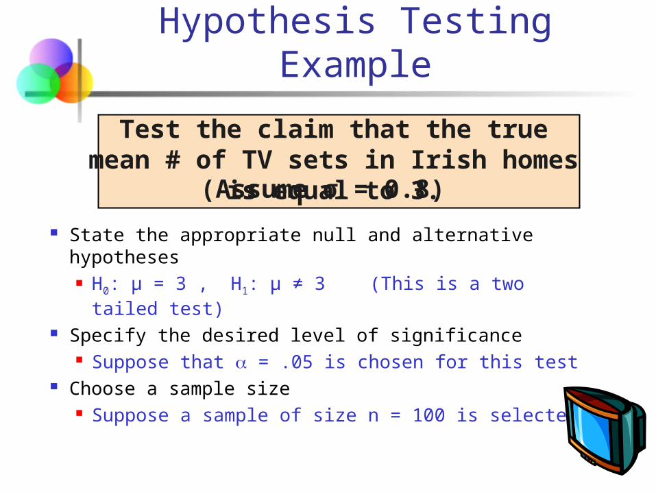
Hypothesis Testing Example
Test the claim that the true mean # of TV sets in Irish homes is equal to 3.
(Assume σ = 0.8)
State the appropriate null and alternativehypotheses H0: μ = 3 , H1: μ ≠ 3 (This is a two tailed test)
Specify the desired level of significance Suppose that = .05 is chosen for this test
Choose a sample size Suppose a sample of size n = 100 is selected
2.0.08
.16
1000.8/
32.84
n/
μXz 0
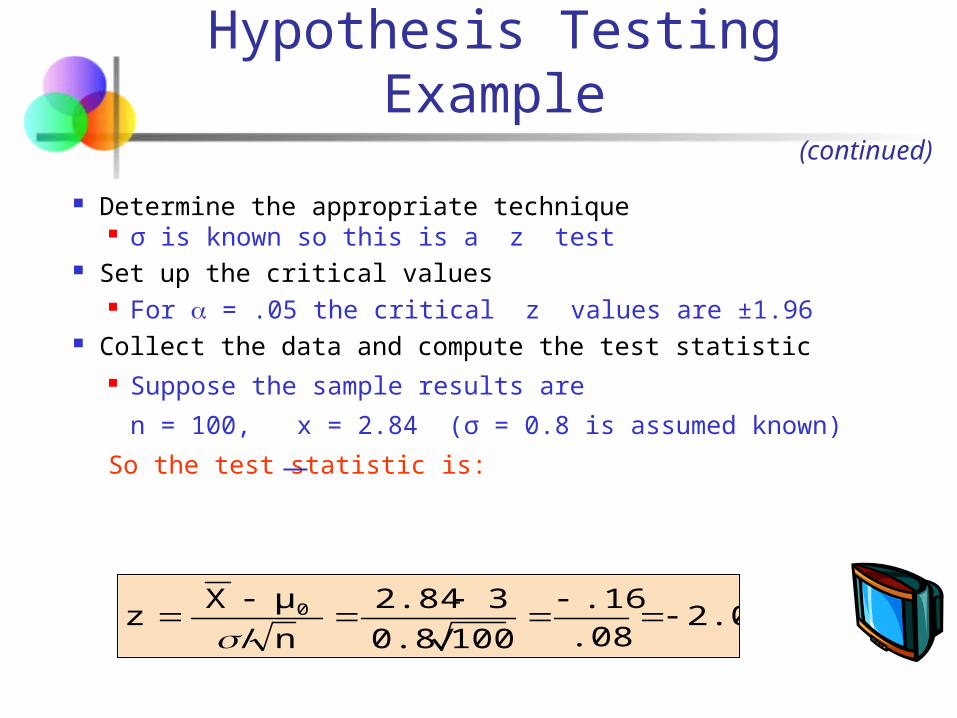
Hypothesis Testing Example
Determine the appropriate technique σ is known so this is a z test
Set up the critical values For = .05 the critical z values are ±1.96
Collect the data and compute the test statistic Suppose the sample results are
n = 100, x = 2.84 (σ = 0.8 is assumed known)
So the test statistic is:
(continued)
Reject H0 Do not reject H0
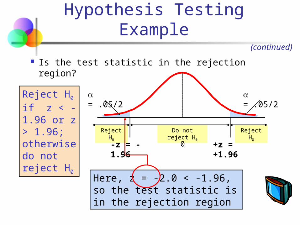
Is the test statistic in the rejection region?
= .05/2
-z = -1.96 0
Reject H0 if z < -1.96 or z > 1.96; otherwise do not reject H0
Hypothesis Testing Example(continued)
= .05/2
Reject H0
+z = +1.96
Here, z = -2.0 < -1.96, so the test statistic is in the rejection region
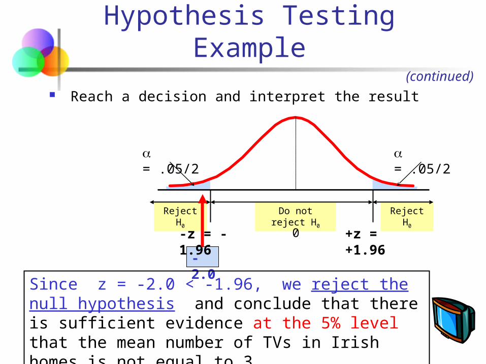
Reach a decision and interpret the result
-2.0
Since z = -2.0 < -1.96, we reject the null hypothesis and conclude that there is sufficient evidence at the 5% level that the mean number of TVs in Irish homes is not equal to 3
Hypothesis Testing Example(continued)
Reject H0 Do not reject H0
= .05/2
-z = -1.96 0
= .05/2
Reject H0
+z = +1.96
.0228
/2 = .025
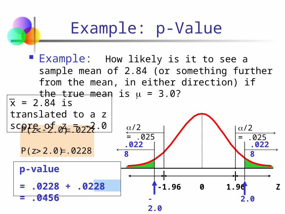
Example: p-Value
Example: How likely is it to see a sample mean of 2.84 (or something further from the mean, in either direction) if the true mean is = 3.0?
-1.96 0
-2.0
.02282.0)P(z
.02282.0)P(z
Z1.96
2.0
x = 2.84 is translated to a z score of z = -2.0
p-value
= .0228 + .0228 = .0456
.0228
/2 = .025
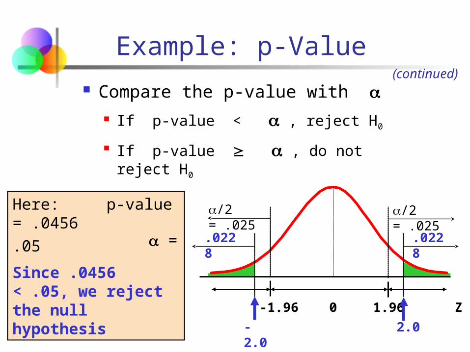
Compare the p-value with If p-value < , reject H0
If p-value , do not reject H0
Here: p-value = .0456 = .05
Since .0456 < .05, we reject the null hypothesis
(continued)
Example: p-Value
.0228
/2 = .025
-1.96 0
-2.0
Z1.96
2.0
.0228
/2 = .025
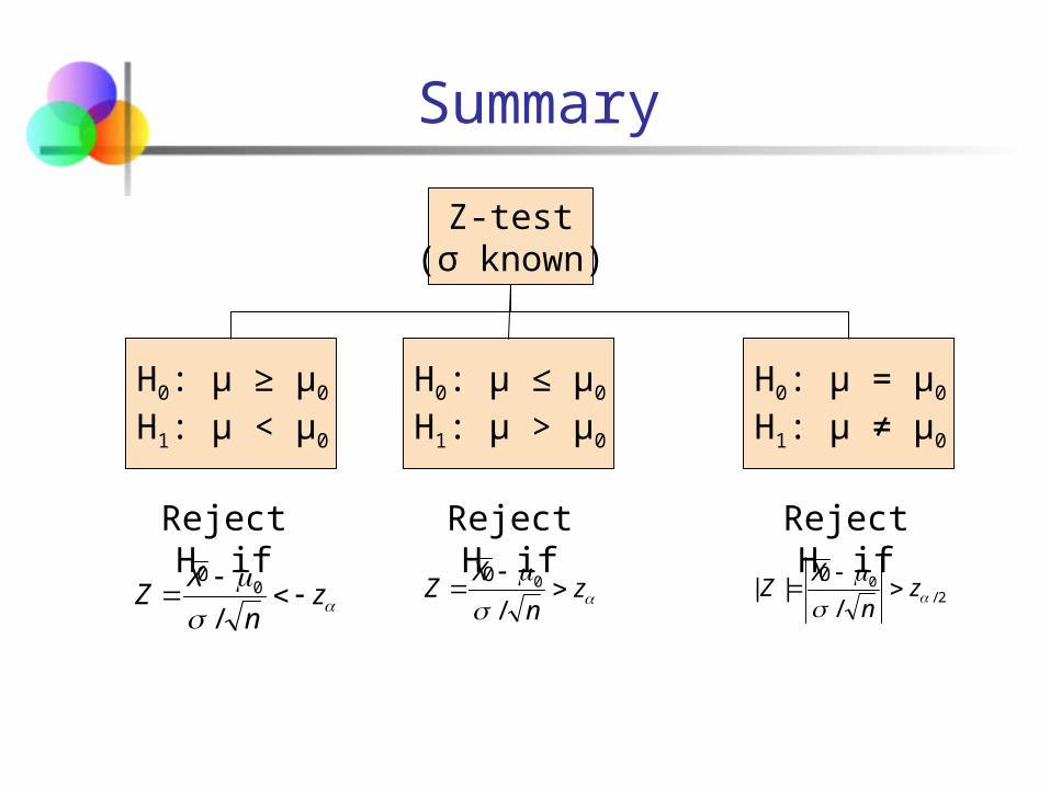
Summary
zn
XZ
/0
zn
XZ
/0
Z-test(σ known)
H0: μ ≥ μ0
H1: μ < μ0
H0: μ ≤ μ0
H1: μ > μ0
H0: μ = μ0
H1: μ ≠ μ0
Reject H0 if Reject H0 if Reject H0 if
2/0
/||
z
n
XZ
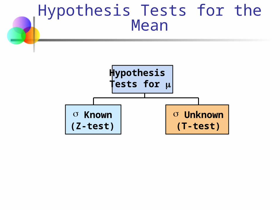
Hypothesis Tests for the Mean
Known(Z-test)
Unknown(T-test)
Hypothesis Tests for
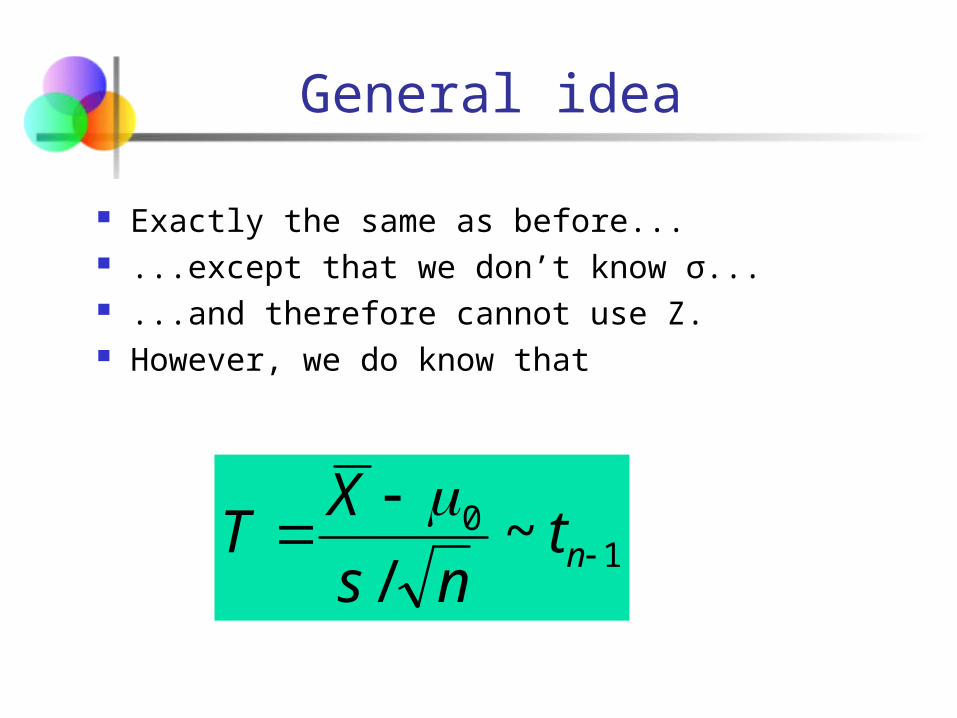
General idea
Exactly the same as before... ...except that we don’t know σ... ...and therefore cannot use Z. However, we do know that
10 ~
/
nt
ns
XT
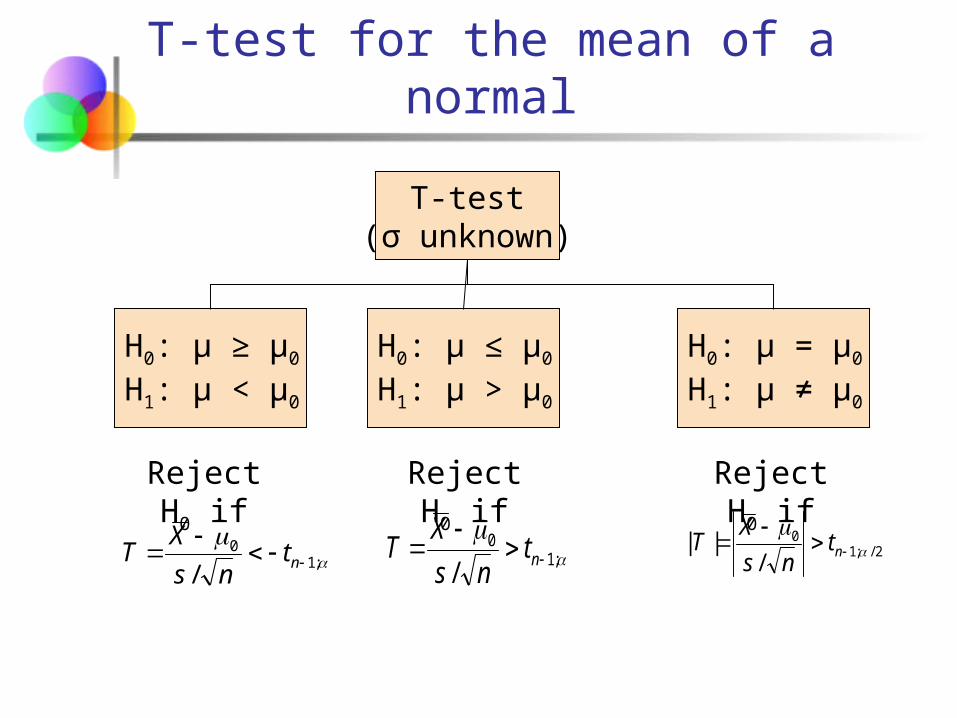
T-test for the mean of a normal
;10
/
nt
ns
XT
;1
0
/
nt
ns
XT
T-test(σ unknown)
H0: μ ≥ μ0
H1: μ < μ0
H0: μ ≤ μ0
H1: μ > μ0
H0: μ = μ0
H1: μ ≠ μ0
Reject H0 if Reject H0 if Reject H0 if
2/;10
/||
nt
ns
XT
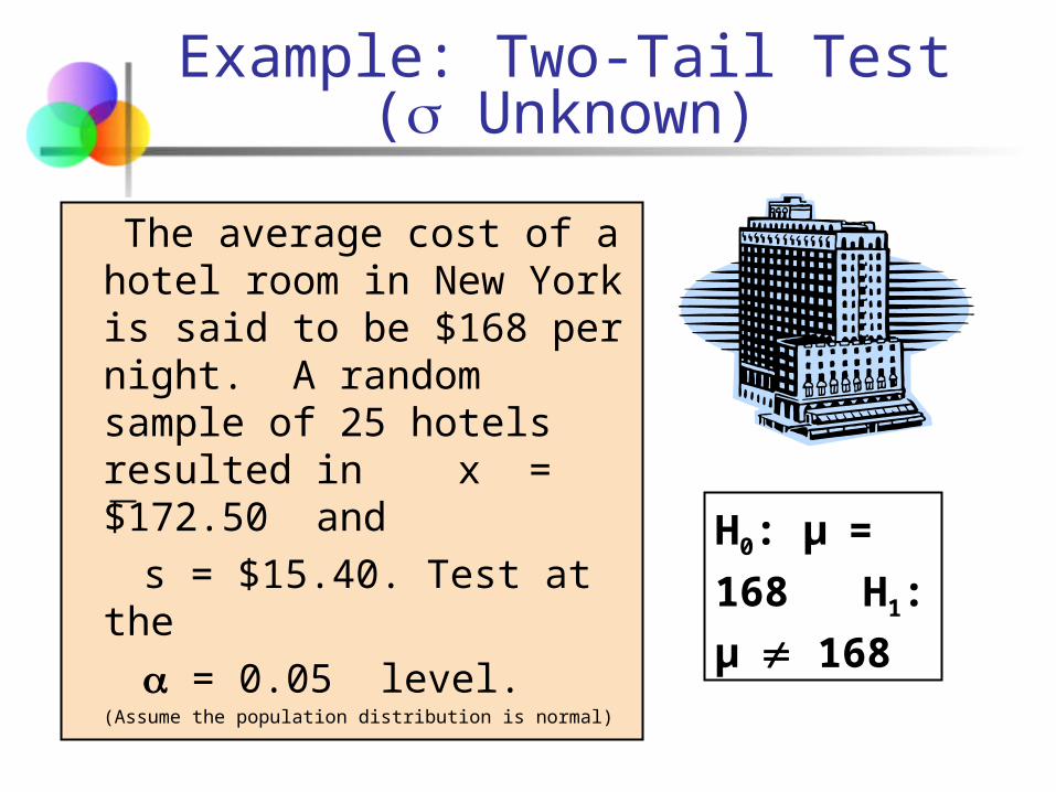
Example: Two-Tail Test( Unknown)
The average cost of a hotel room in New York is said to be $168 per night. A random sample of 25 hotels resulted in x = $172.50 and
s = $15.40. Test at the
= 0.05 level.(Assume the population distribution is normal)
H0: μ=
168 H1:
μ 168
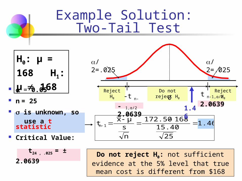
= 0.05
n = 25
is unknown, so use a t statistic
Critical Value:
t24 , .025 = ± 2.0639
Example Solution: Two-Tail Test
Do not reject H0: not sufficient evidence at the 5% level that true mean cost is different from
$168
Reject H0Reject H0
/2=.025
-t n-1,α/2
Do not reject H0
0
/2=.025
-2.0639 2.0639
1.46
25
15.40168172.50
n
sμx
t 1n
1.46
H0: μ=
168 H1:
μ 168t n-1,α/2
Tests of the Population Proportion
Involves categorical variables
Two possible outcomes “Success” (a certain characteristic is present)
“Failure” (the characteristic is not present)
Fraction or proportion of the population in the “success” category is denoted by p
Assume sample size is large
Proportions
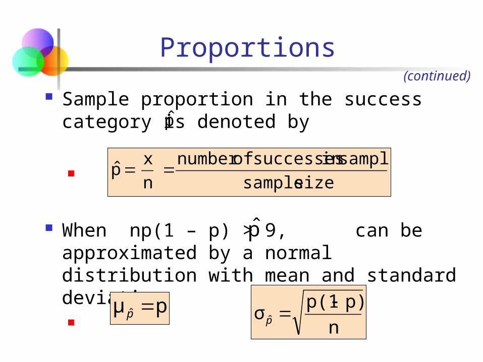
Sample proportion in the success category is denoted by
When np(1 – p) > 9, can be approximated by a normal distribution with mean and standard deviation
sizesample
sampleinsuccessesofnumber
n
xp̂
pμ ˆ pn
p)p(1σ ˆ
p
(continued)
p̂
p̂
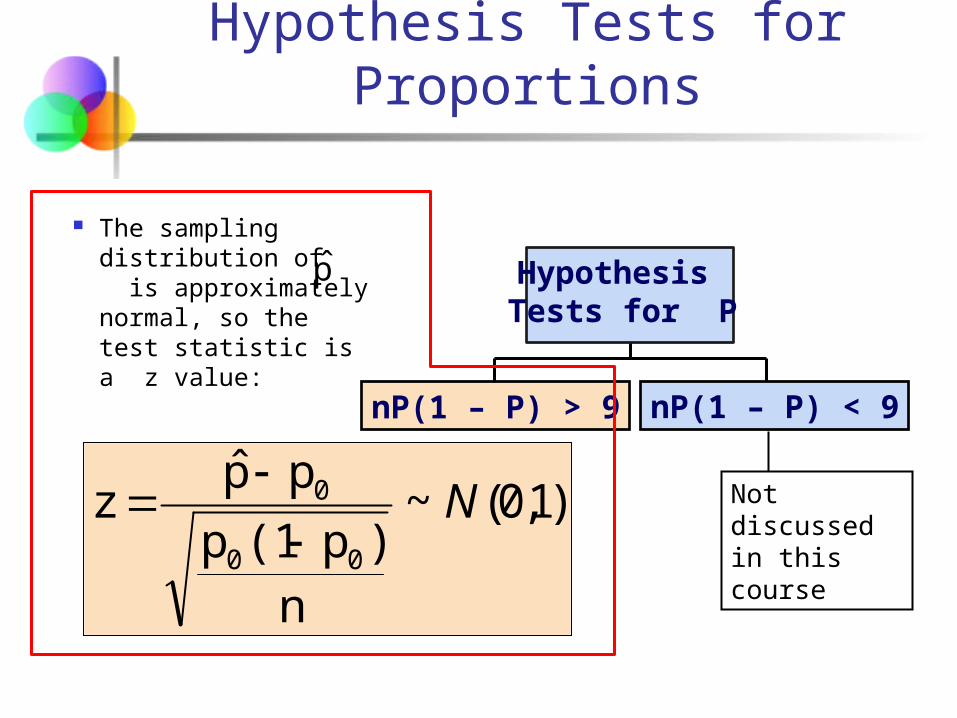
The sampling distribution of is approximately normal, so the test statistic is a z value:
Hypothesis Tests for Proportions
)1,0(~
n)p(1p
pp̂z
00
0 N
nP(1 – P) > 9
Hypothesis Tests for P
Not discussed in this course
p̂
nP(1 – P) < 9
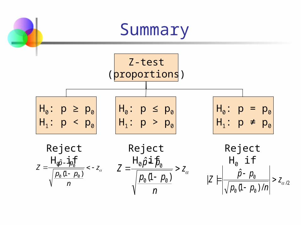
Summary
z
npp
ppZ
)1(
ˆ
00
0
2/
00
0
/)1(
ˆ|| z
npp
ppZ
Z-test(proportions)
H0: p ≥ p0
H1: p < p0
H0: p ≤ p0
H1: p > p0
H0: p = p0
H1: p ≠ p0
Reject H0 if Reject H0 if Reject H0 if
z
npp
ppZ
)1(
ˆ
00
0
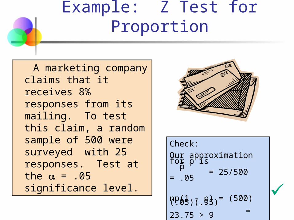
Example: Z Test for Proportion
A marketing company claims that it receives 8% responses from its mailing. To test this claim, a random sample of 500 were surveyed with 25 responses. Test at the = .05 significance level.
Check:
Our approximation for p is = 25/500 = .05
np(1 - p) = (500)(.05)(.95) = 23.75 > 9
p̂
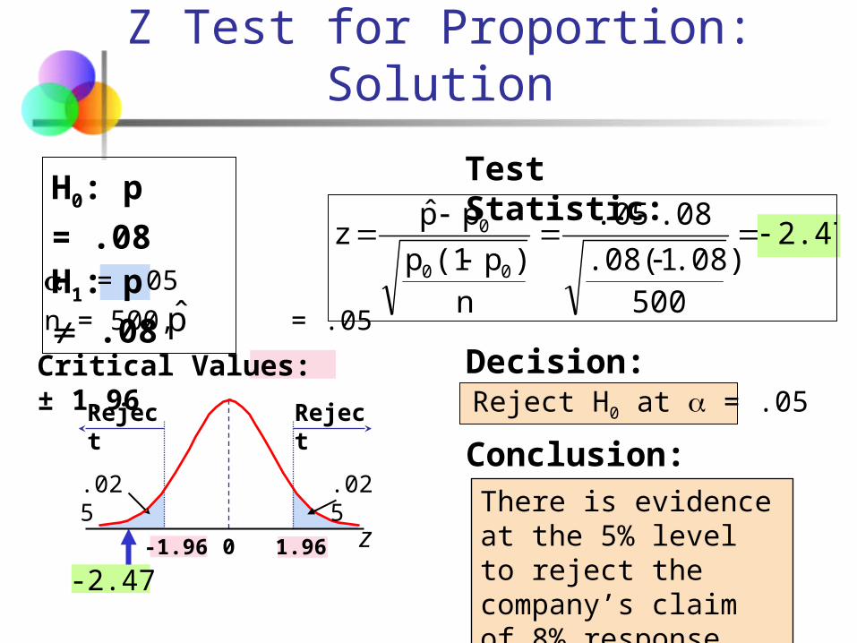
Z Test for Proportion: Solution
= .05
n = 500, = .05
Reject H0 at = .05
H0: p = .08
H1: p
.08
Critical Values: ± 1.96
Test Statistic:
Decision:
Conclusion:
z0
Reject Reject
.025.025
1.96
-2.47
There is evidence at the 5% level to reject the company’s claim of 8% response rate.
2.47
500.08).08(1
.08.05
n)p(1p
pp̂z
00
0
-1.96
p̂
Do not reject H0
Reject H0Reject H0
/2 = .025
1.960
Z = -2.47
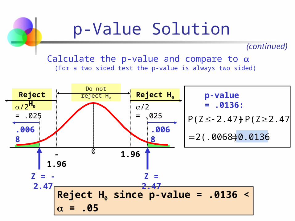
Calculate the p-value and compare to (For a two sided test the p-value is always two sided)
(continued)
0.01362(.0068)
2.47)P(Z2.47)P(Z
p-value = .0136:
p-Value Solution
Reject H0 since p-value = .0136 < = .05
Z = 2.47
-1.96
/2 = .025
.0068.0068
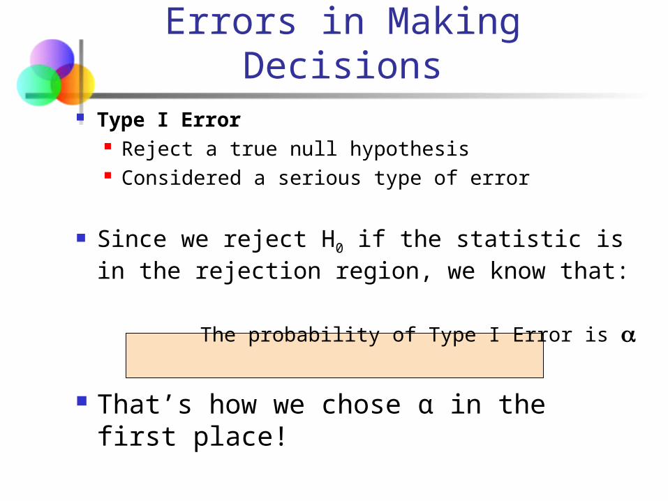
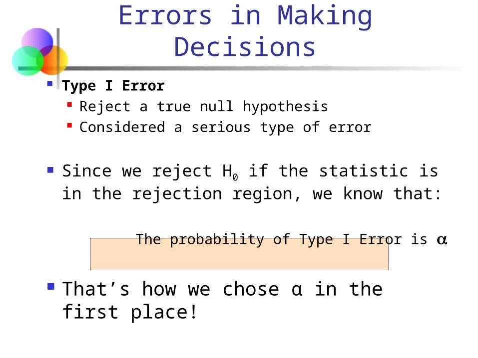
Errors in Making Decisions Type I Error
Reject a true null hypothesis Considered a serious type of error
Since we reject H0 if the statistic is in the rejection region, we know that:
The probability of Type I Error is
That’s how we chose α in the first place!
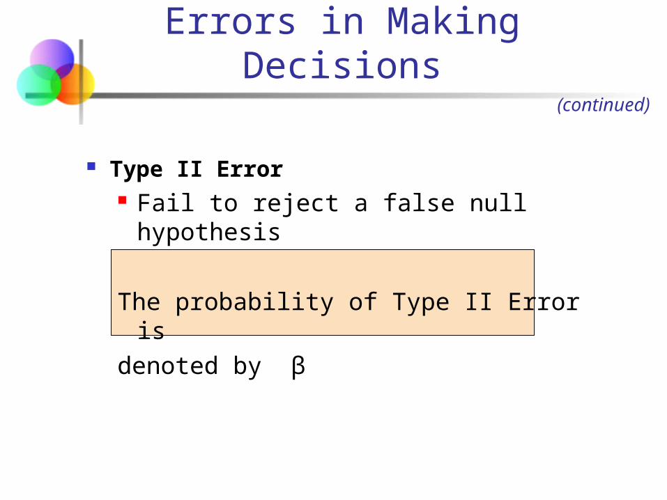
Errors in Making Decisions
Type II Error Fail to reject a false null hypothesis
The probability of Type II Error is β
(continued)
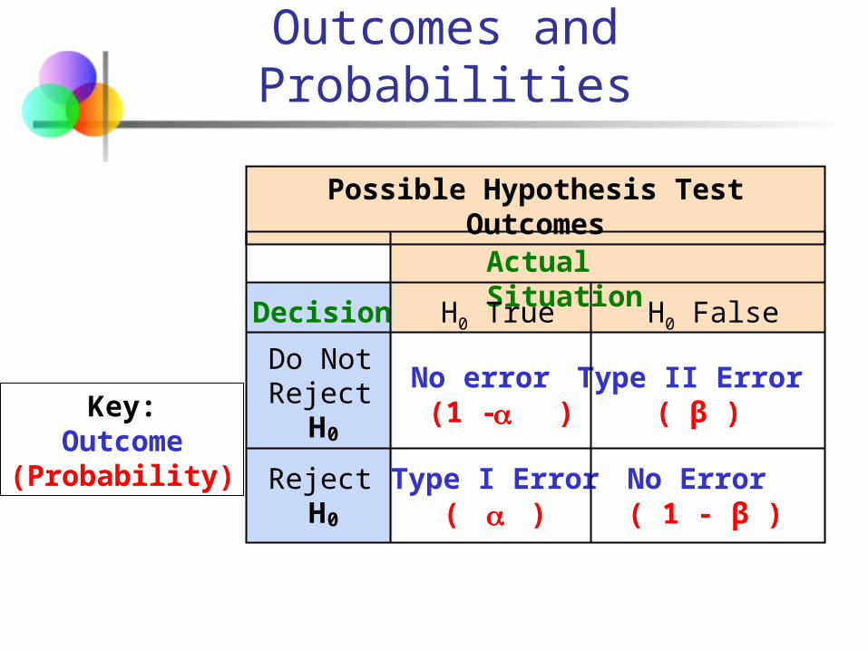
Outcomes and Probabilities
Actual SituationDecision
Do NotReject
H0
No error (1 - )
Type II Error ( β )
RejectH0
Type I Error( )
Possible Hypothesis Test Outcomes
H0 False H0 True
Key:Outcome
(Probability) No Error ( 1 - β )

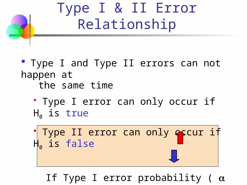
Type I & II Error Relationship
Type I and Type II errors can not happen at the same time
Type I error can only occur if H0 is true
Type II error can only occur if H0 is false
If Type I error probability ( ) , then
Type II error probability ( β )
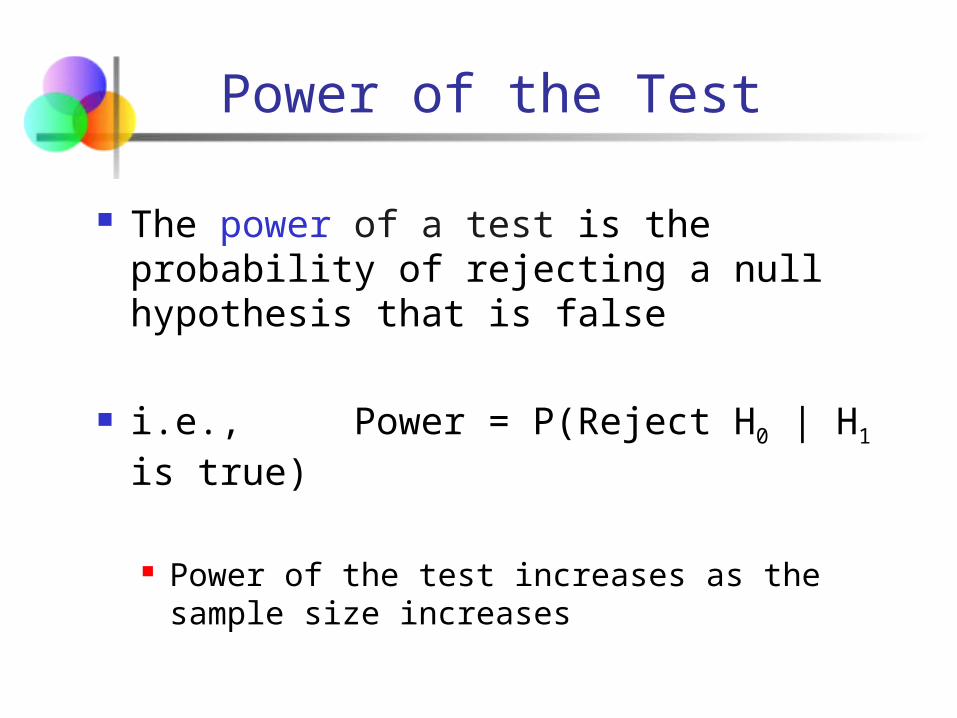
Power of the Test
The power of a test is the probability of rejecting a null hypothesis that is false
i.e., Power = P(Reject H0 | H1 is true)
Power of the test increases as the sample size increases

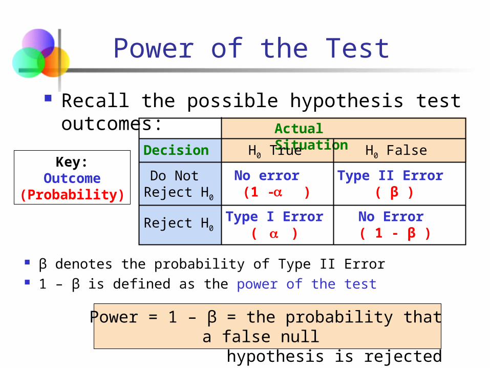
Recall the possible hypothesis test outcomes:Actual Situation
Decision
Do Not Reject H0
No error (1 - )
Type II Error ( β )
Reject H0Type I Error
( )
H0 False H0 TrueKey:
Outcome(Probability)
No Error ( 1 - β )
β denotes the probability of Type II Error 1 – β is defined as the power of the test
Power = 1 – β = the probability that a false null hypothesis is rejected
Power of the Test
Type II Error
or
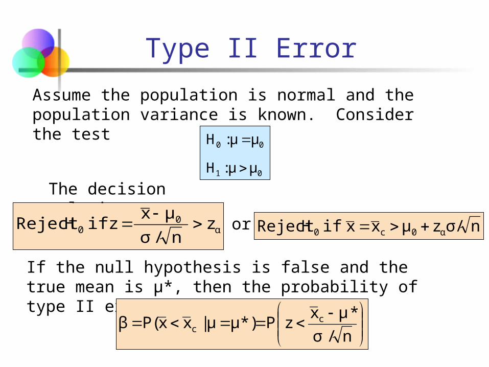
The decision rule is:
α0
0 zn/σ
μxz if HReject
00 μμ:H
01 μμ:H
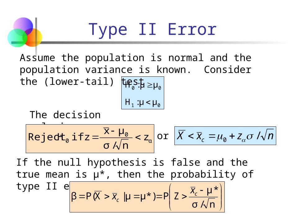
Assume the population is normal and the population variance is known. Consider the test
nσ/zμxx if HReject α0c0
If the null hypothesis is false and the true mean is μ*, then the probability of type II error is
n/σ
*μxzPμ*)μ|xxP(β c
c
Reject H0: μ 52
Do not reject H0 : μ 52
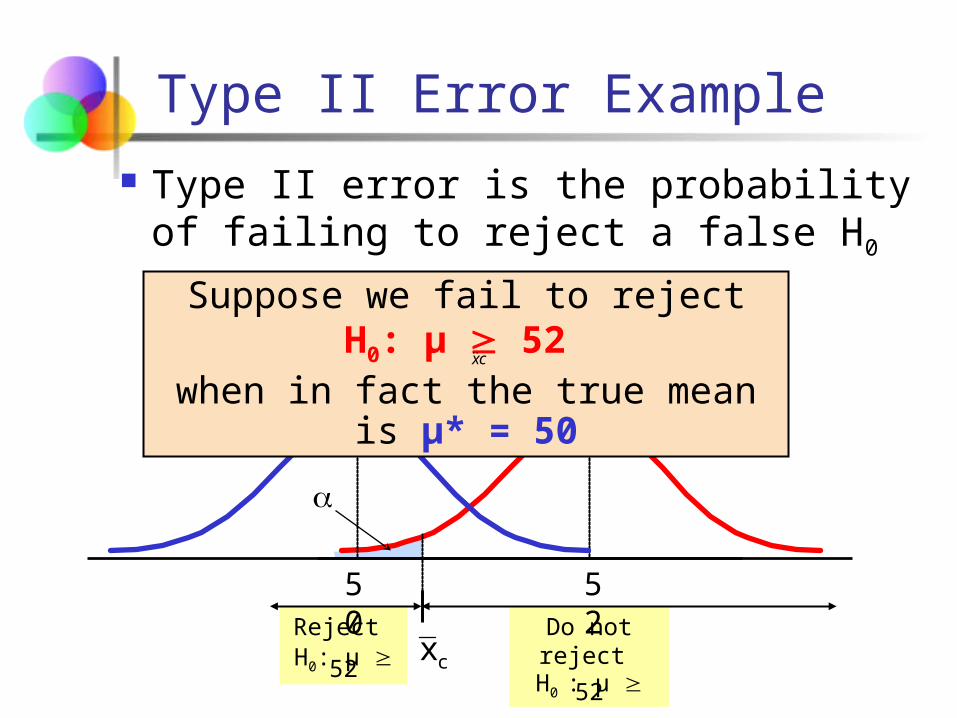
Type II Error Example
Type II error is the probability of failing to reject a false H0
5250
Suppose we fail to reject H0: μ 52 when in fact the true mean is μ* = 50
cx
cx
Reject H0: μ 52
Do not reject H0 : μ 52
Type II Error Example
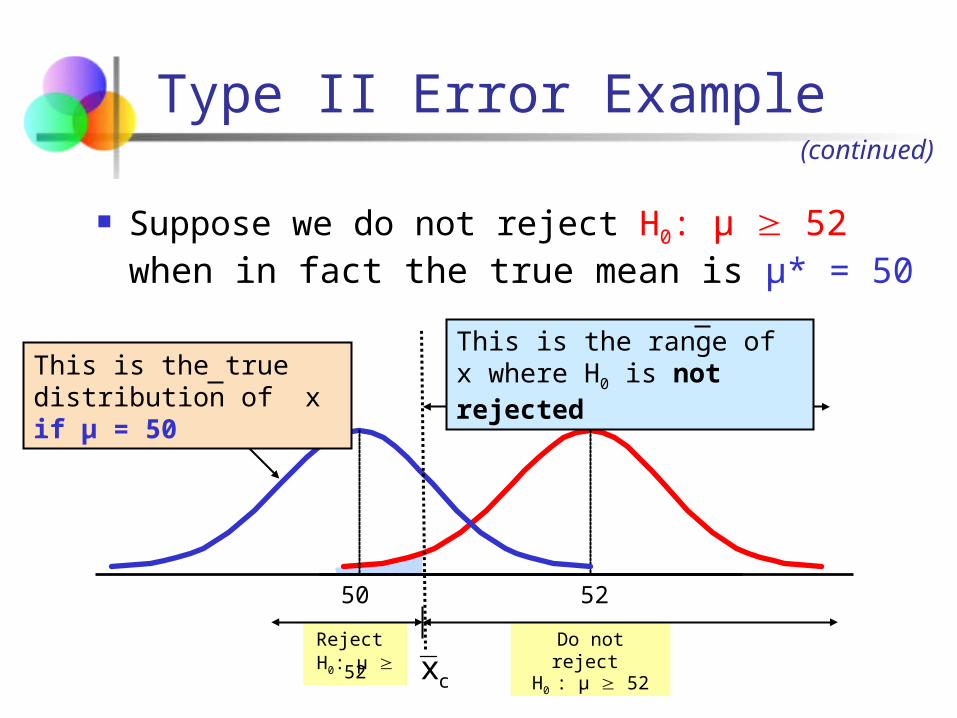
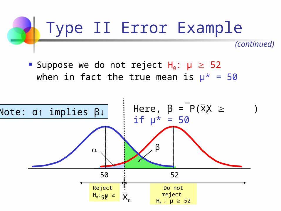
Suppose we do not reject H0: μ 52 when in fact the true mean is μ* = 50
5250
This is the true distribution of x if μ = 50
This is the range of x where H0 is not rejected
(continued)
cx
Reject H0: μ 52
Do not reject H0 : μ 52
Type II Error Example
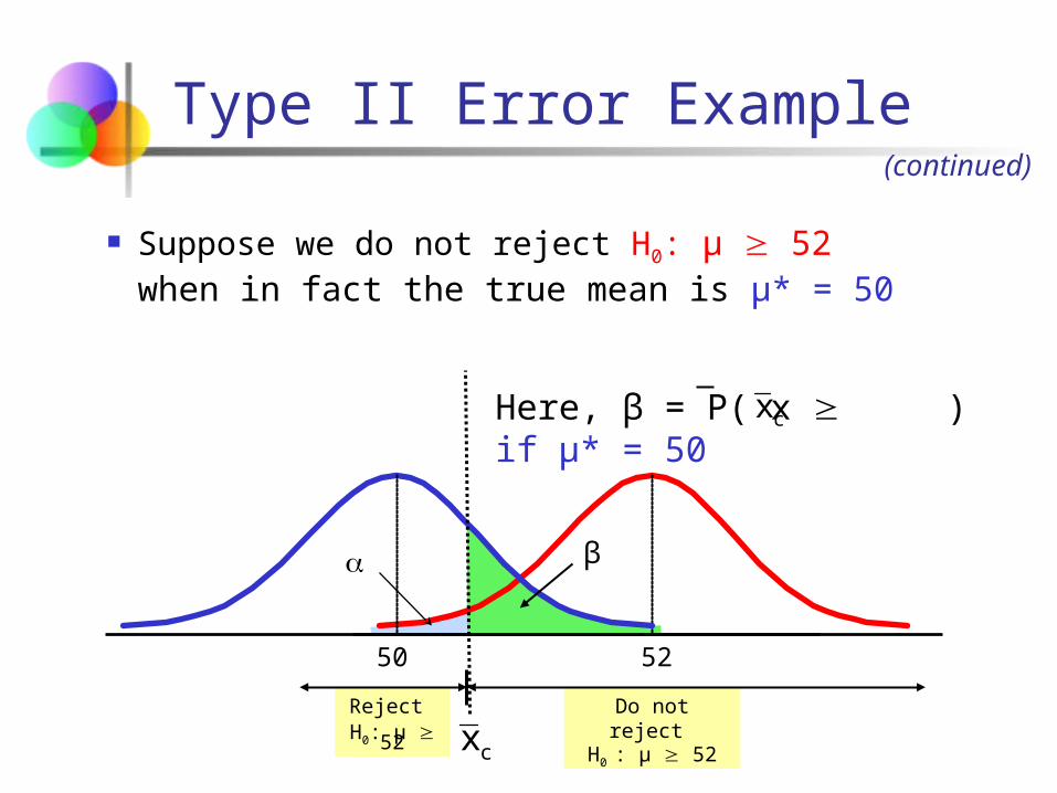
Suppose we do not reject H0: μ 52 when in fact the true mean is μ* = 50
5250
β
Here, β = P( x ) if μ* = 50
(continued)
cx
cx
Reject H0: μ 52
Do not reject H0 : μ 52
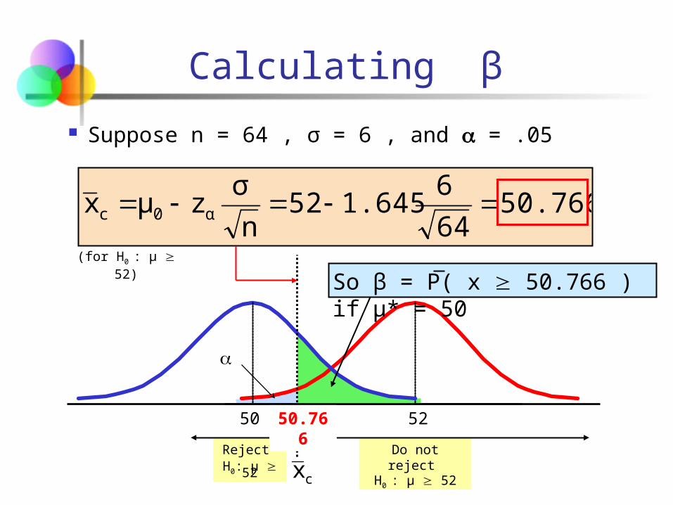
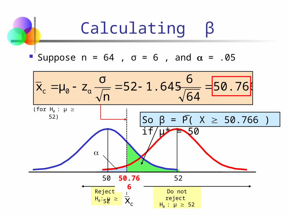
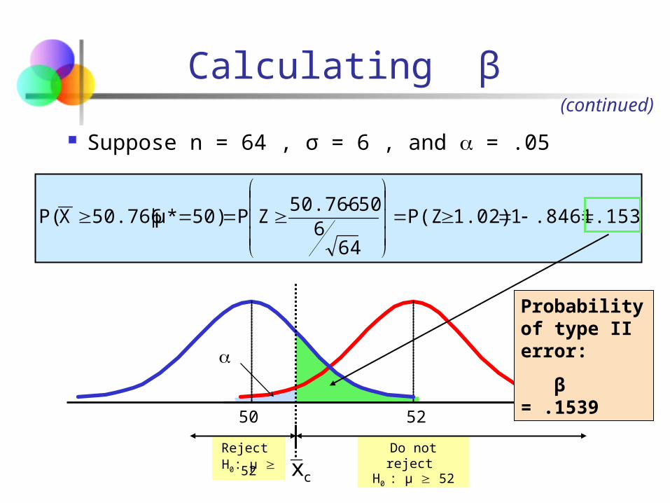
Suppose n = 64 , σ = 6 , and = .05
5250
So β = P( x 50.766 ) if μ* = 50
Calculating β
50.76664
61.64552
n
σzμx α0c
(for H0 : μ 52)
50.766
cx
Reject H0: μ 52
Do not reject H0 : μ 52
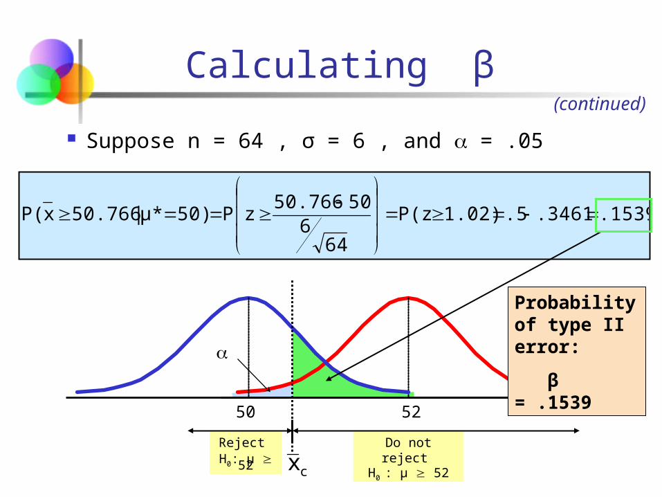
.1539.3461.51.02)P(z
646
5050.766zP50)μ*|50.766xP(
Suppose n = 64 , σ = 6 , and = .05
5250
Calculating β(continued)
Probability of type II error:
β = .1539
cx

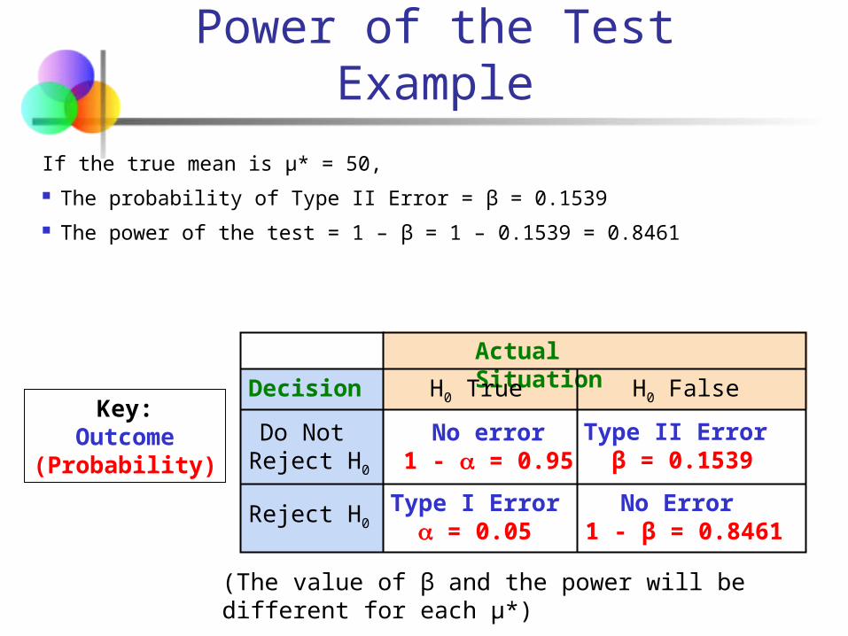
If the true mean is μ* = 50,
The probability of Type II Error = β = 0.1539
The power of the test = 1 – β = 1 – 0.1539 = 0.8461
Power of the Test Example
Actual Situation
Decision
Do Not Reject H0
No error1 - = 0.95
Type II Error β = 0.1539
Reject H0Type I Error
= 0.05
H0 False H0 TrueKey:
Outcome(Probability)
No Error 1 - β = 0.8461
(The value of β and the power will be different for each μ*)

The Godfather
Some of the Dons of important mafia families claim that DonCorleone does not bring in the promised $5mln in “transactions”. Corleone orders his consiglieri to investigate.
Tom Hagen asks you
You can sample 16 transactions
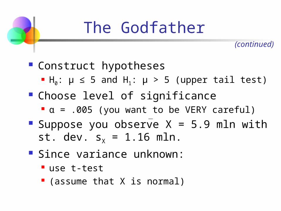
The Godfather
Construct hypotheses H0: μ ≤ 5 and H1: μ > 5 (upper tail test)
Choose level of significance α = .005 (you want to be VERY careful)
Suppose you observe X = 5.9 mln with st. dev. sX = 1.16 mln.
Since variance unknown: use t-test (assume that X is normal)
(continued)
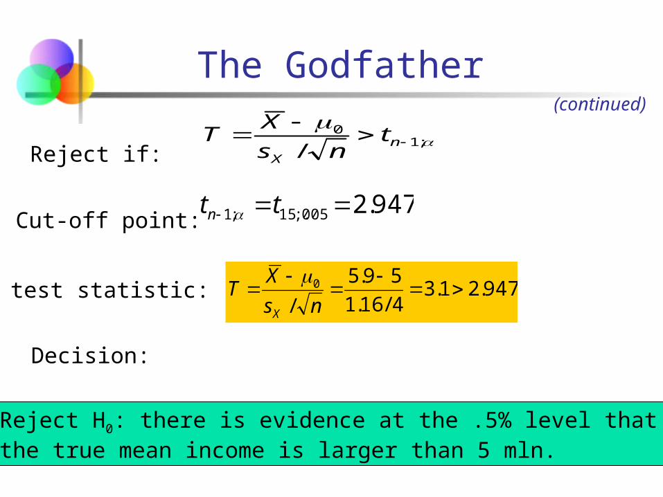
The Godfather
;10
/
n
X
tns
XT
947.2005;.15;1 ttn
(continued)
Reject if:
Cut-off point:
test statistic: 947.21.34/16.1
59.5
/0
ns
XT
X
Reject H0: there is evidence at the .5% level thatthe true mean income is larger than 5 mln.
Decision:
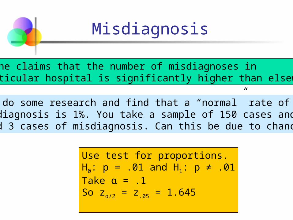
Misdiagnosis
Someone claims that the number of misdiagnoses ina particular hospital is significantly higher than elsewhere.
You do some research and find that a “normal” rate ofmisdiagnosis is 1%. You take a sample of 150 cases and find 3 cases of misdiagnosis. Can this be due to chance?
Use test for proportions.H0: p = .01 and H1: p ≠ .01Take α = .1So zα/2 = z.05 = 1.645
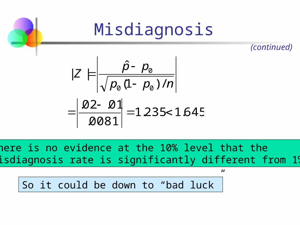
Misdiagnosis(continued)
645.1235.10081.
01.02.
/)1(
ˆ||
00
0
npp
ppZ
There is no evidence at the 10% level that the misdiagnosis rate is significantly different from 1%.
So it could be down to “bad luck”
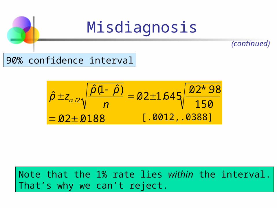
Misdiagnosis(continued)
90% confidence interval
0188.02.150
98.*02.645.102.
)ˆ1(ˆˆ 2/
n
ppzp
[.0012,.0388]
Note that the 1% rate lies within the interval.That’s why we can’t reject.
Errors in Making Decisions Type I Error
Reject a true null hypothesis Considered a serious type of error
Since we reject H0 if the statistic is in the rejection region, we know that:
The probability of Type I Error is
That’s how we chose α in the first place!
Errors in Making Decisions
Type II Error Fail to reject a false null hypothesis
The probability of Type II Error is
denoted by β
(continued)

Outcomes and Probabilities
Actual SituationDecision
Do NotReject
H0
No error (1 - )
Type II Error ( β )
RejectH0
Type I Error( )
Possible Hypothesis Test Outcomes
H0 False H0 True
Key:Outcome
(Probability) No Error ( 1 - β )
Type I & II Error Relationship
Type I and Type II errors can not happen at the same time
Type I error can only occur if H0 is true
Type II error can only occur if H0 is false
If Type I error probability ( ) , then
Type II error probability ( β )

Power of the Test
The power of a test is the probability of rejecting a null hypothesis that is false
i.e., Power = P(Reject H0 | H1 is true)
Power of the test increases as the sample size increases
Recall the possible hypothesis test outcomes:Actual Situation
Decision
Do Not Reject H0
No error (1 - )
Type II Error ( β )
Reject H0Type I Error
( )
H0 False H0 TrueKey:
Outcome(Probability)
No Error ( 1 - β )
β denotes the probability of Type II Error 1 – β is defined as the power of the test
Power = 1 – β = the probability that a false null hypothesis is rejected
Power of the Test
Type II Error
The decision rule is:
α0
0 zn/σ
μxz if HReject
00 μμ:H
01 μμ:H
Assume the population is normal and the population variance is known. Consider the (lower-tail) test
If the null hypothesis is false and the true mean is μ*, then the probability of type II error is
n/σ
*μZPμ*)μ|XP(β c
c
xx
or nzxX c /0

Reject H0: μ 52
Do not reject H0 : μ 52
Type II Error Example
Type II error is the probability of failing to reject a false H0
5250
Suppose we fail to reject H0: μ 52 when in fact the true mean is μ* = 50
cx
cx

Reject H0: μ 52
Do not reject H0 : μ 52
Type II Error Example
Suppose we do not reject H0: μ 52 when in fact the true mean is μ* = 50
5250
This is the true distribution of X if μ = 50
This is the range of x where H0 is not rejected
(continued)
cx
Reject H0: μ 52
Do not reject H0 : μ 52
Type II Error Example
Suppose we do not reject H0: μ 52 when in fact the true mean is μ* = 50
5250
β
Here, β = P( X ) if μ* = 50
(continued)
cx
cxNote: α↑ implies β↓
Reject H0: μ 52
Do not reject H0 : μ 52
Suppose n = 64 , σ = 6 , and = .05
5250
So β = P( X 50.766 ) if μ* = 50
Calculating β
50.76664
61.64552
n
σzμx α0c
(for H0 : μ 52)
50.766
cx
Reject H0: μ 52
Do not reject H0 : μ 52
.1539.846111.02)P(Z
646
5050.766ZP50)μ*|50.766XP(
Suppose n = 64 , σ = 6 , and = .05
5250
Calculating β(continued)
Probability of type II error:
β = .1539
cx
If the true mean is μ* = 50,
The probability of Type II Error = β = 0.1539
The power of the test = 1 – β = 1 – 0.1539 = 0.8461
Power of the Test Example
Actual Situation
Decision
Do Not Reject H0
No error1 - = 0.95
Type II Error β = 0.1539
Reject H0Type I Error
= 0.05
H0 False H0 TrueKey:
Outcome(Probability)
No Error 1 - β = 0.8461
(The value of β and the power will be different for each μ*)
Topic Summary
Addressed hypothesis testing methodology
Performed Z Test for the mean (σ known)
Discussed critical value and p-value approaches to hypothesis testing
Performed one-tail and two-tail tests
Performed t test for the mean (σ unknown)
Performed Z test for the proportion
Discussed type II error and power of the test