topics in mathematical physics - higher...
TRANSCRIPT
Topics in Mathematical Physics
Prof. V.Palamodov
Spring semester 2002
Contents
Chapter 1. Differential equations of Mathematical Physics
1.1 Differential equations of elliptic type
1.2 Diffusion equations
1.3 Wave equations
1.4 Systems
1.5 Nonlinear equations
1.6 Hamilton-Jacobi theory
1.7 Relativistic field theory
1.8 Classification
1.9 Initial and boundary value problems
1.10 Inverse problems
Chapter 2. Elementary methods
2.1 Change of variables
2.2 Bilinear integrals
2.3 Conservation laws
2.4 Method of plane waves
2.5 Fourier transform
2.6 Theory of distributions
Chapter 3. Fundamental solutions
3.1 Basic definition and properties
3.2 Fundamental solutions for elliptic operators
3.3 More examples
3.4 Hyperbolic polynomials and source functions
3.5 Wave propagators
3.6 Inhomogeneous hyperbolic operators
3.7 Riesz groups
Chapter 4. The Cauchy problem
4.1 Definitions
4.2 Cauchy problem for distributions
4.3 Hyperbolic Cauchy problem
4.4 Solution of the Cauchy problem for wave equations
4.5 Domain of dependence
2
Chapter 5. Helmholtz equation and scattering
5.1 Time-harmonic waves
5.2 Source functions
5.3 Radiation conditions
5.4 Scattering on obstacle
5.5 Interference and diffraction
Chapter 6. Geometry of waves
6.1 Wave fronts
6.2 Hamilton-Jacobi theory
6.3 Geometry of rays
6.4 An integrable case
6.5 Legendre transformation and geometric duality
6.6 Fermat principle
6.7 The major Huygens principle
6.8 Geometrical optics
6.9 Caustics
6.10 Geometrical conservation law
Chapter 7. The method of Fourier integrals
7.1 Elements of symplectic geometry
7.2 Generating functions
7.3 Fourier integrals
7.4 Lagrange distributions
7.5 Hyperbolic Cauchy problem revisited
Chapter 8. Electromagnetic waves
8.1 Vector analysis
8.2 Maxwell equations
8.3 Harmonic analysis of solutions
8.4 Cauchy problem
8.5 Local conservation laws
3
Chapter 1
Differential equations of
Mathematical Physics
1.1 Differential equations of elliptic type
Let X be an Euclidean space of dimension n with a coordinate systemx1, ..., xn.
• The Laplace equation is
∆u = 0, ∆.=
∂2
∂x21
+ ...+∂2
∂x2n
∆ is called the Laplace operator. A solution in a domain Ω ⊂ Xis called harmonic function in Ω. It describes a stable membrane,electrostatic or gravity field.
• The Helmholtz equation
(
∆+ ω2)
u = 0
For n = 1 it is called the equation of harmonic oscillator. A solution isa time-harmonic wave in homogeneous space.
• Let σ be a function in Ω; the equation
〈∇, σ∇〉 u = f, ∇.=
(
∂
∂x1
, ...,∂
∂xn
)
1
is the electrostatic equation with the conductivity σ. We have 〈∇, σ∇〉 u =σ∆u+ 〈∇σ,∇u〉 .
• Stationary Schrodinger equation(
−h2
2m∆+ V (x)
)
ψ = Eψ
E is the energy of a particle.
1.2 Diffusion equations
• The equation∂u (x, t)
∂t− d2∆xu (x, t) = f
in X × R describes propagation of heat in X with the source densityf .
• The equation
ρ∂u
∂t− 〈∇, p∇〉 u− qu = f
describes diffusion of small particles.
• The Fick equation
∂
∂tc+ div (wc) = D∆c+ f
for convective diffusion accompanied by a chemical reaction; c is theconcentration, f is the production of a specie, w is the volume velocity,D is the diffusion coefficient.
• The Schrodinger equation(
ıh∂
∂t+
h2
2m∆− V (x)
)
ψ (x, t) = 0
where h = 1.054... × 10−27 erg · sec is the Plank constant. The wavefunction ψ describes motion of a particle of mass m in the exterior fieldwith the potential V. The density |ψ (x, t)|2 dx is the probability to findthe particle in the point x at the time t.
2
1.3 Wave equations
1.3.1 The case dim X = 1
• The equation(
∂2
∂t2− v2 (x)
∂2
∂x2
)
u (x, t) = 0
is called D’Alembert equation or the wave equation for one spacialvariable x and velocity v.
• The telegraph equations
∂V
∂x+ L
∂I
∂t+R
∂I
∂x= 0,
∂I
∂x+ C
∂V
∂t+GV = 0
V, I are voltage and current in a conducting line, L,C,R,G are induc-tivity, capacity, resistivity and leakage conductivity of the line.
• The equation of oscillation of a slab
∂2u
∂t2+ γ2∂
4u
∂x4= 0
1.3.2 The case dim X = 2, 3
• The wave equation in an isotropic medium (membrane equation):
(
∂2
∂t2− v2 (x)∆
)
u (x, t) = 0
• The acoustic equation
∂2u
∂t2−⟨
∇, v2∇⟩
u = 0, ∇ = (∂1, ..., ∂n)
• Wave equation in an anisotropic medium:
(
∂2
∂t2−∑
aij (x)∂2
∂xi∂xj−∑
bi (x)∂u
∂xi
)
u (x, t) = f (x, t)
3
• The transport equation
∂u
∂t+ θ
∂u
∂x+ a (x)u− b (x)
∫
S(X)
η (〈θ, θ′〉 , x) u (x, θ′, t) dθ′ = q
It describes the density u = u (x, θ, t) of particles at a point (x, t) ofspace-time moving in direction θ.
• The Klein-Gordon-Fock equation(
∂2
∂t2− c2∆+m2
)
u (x, t) = 0
where c is the light speed. A relativistic scalar particle of the mass m.
1.4 Systems
• The Maxwell system:
div (µH) = 0, rotE = −1
c
∂
∂t(µH) ,
div (εE) = 4πρ, rotH =1
c
∂
∂t(εE) +
4π
cI,
E and H are the electric and magnetic fields, ρ is the electric chargeand I is the current; ε, µ are electric permittivity and magnetic per-meability, respectively, v2 = c2/εµ. In a non-isotropic medium ε, µ aresymmetric positively defined matrices.
• The elasticity system
ρ∂
∂tui =
∑ ∂
∂xjvij
where U (x, t) = (u1, u2, u3) is the displacement evaluated in the tan-gent bundle T (X) and vij is the stress tensor:
vij = λδij∂
∂xkuk + µ
(
∂
∂xjui +
∂
∂xiuj
)
, i, j = 1, 2, 3
ρ is the density of the elastic medium in a domain Ω ⊂ X; λ, µ are theLame coefficients (isotropic case).
4
1.5 Nonlinear equations
1.5.1 dim X = 1
• The equation of shock waves
∂u
∂t+ u
∂u
∂x= 0
• Burgers equation for shock waves with dispersion
∂u
∂t+ u
∂u
∂x− b
∂2u
∂x2= 0
• The Korteweg-de-Vries (shallow water) equation
∂u
∂t+ 6u
∂u
∂x+∂3u
∂x3= 0
• Boussinesq equation
∂2u
∂t2−∂2u
∂x2− 6u
∂2u
∂x2−∂4u
∂x4= 0
1.5.2 dim X = 2, 3
• The nonlinear Schrodinger equation
ıh∂u
∂t+
h2
2m∆u± |u|2 u = 0
• Nonlinear wave equation(
∂2
∂t2− v2∆
)
u+ f (u) = 0
where f is a nonlinear function, f.e. f (u) = ±u3 or sinu.
• The system of hydrodynamics (gas dynamic)
∂ρ
∂t+ div (ρv) = f
∂v
∂t+ 〈v, grad v〉+
1
ρgrad p = F
Φ (p, ρ) = 0
5
for the velocity vector v = (v1, v2, v3), the density function ρ and thepressure p of the liquid. They are called continuity, Euler and the stateequation, respectively.
• The Navier-Stokes system
∂ρ
∂t+ div (ρV ) = f
∂v
∂t+ 〈v, grad v〉+ α∆v +
1
ρgrad p = F
Φ (p, ρ) = 0
where α is the viscosity coefficient.
• The system of magnetic hydrodynamics
divB = 0,∂B
∂t− rot (u×B) = 0
ρ∂u
∂t+ ρ 〈u,∇〉 u+ grad p− µ−1 rotB ×B = 0,
∂ρ
∂t+ div (ρu) = 0
where u is the velocity, ρ the density of the liquid, B = µH is themagnetic induction, µ is the magnetic permeability.
1.6 Hamilton-Jacobi theory
• The Hamilton-Jacobi (Eikonal) equation
aµν∂µφ∂νφ = v−2 (x)
• Hamilton-Jacobi system
∂x
∂τ= H ′
ξ (x, ξ) ,∂ξ
∂τ= −H ′
x (x, ξ)
where H is called the Hamiltonian function.
• Euler-Lagrange equation
∂L
∂x−
d
dt
∂L
∂·x
= 0
where L = L (t, x,.x) , x = (x1, ..., xn) is the Lagrange function.
6
1.7 Relativistic field theory
1.7.1 dim X = 3
• The Schrodinger equation in a magnetic field
ıh∂u
∂t+
h2
2m
(
∂j −e
cAj
)2
ψ − eV ψ = 0
• The Dirac equation(
ı
3∑
0
γµ∂µ −mI
)
ψ = 0
where ∂0 = ∂/∂t, ∂k = ∂/∂xk, k = 1, 2, 3 and γk, k = 0, 1, 2, 3 are4× 4 matrices (Dirac matrices):
(
σ0 00 −σ0
)
,
(
0 σ1
−σ1 0
)
,
(
0 σ2
−σ2 0
)
,
(
0 σ3
−σ3 0
)
and
σ0 =
(
1 00 1
)
, σ1 =
(
0 11 0
)
, σ2 =
(
0 −ıı 0
)
, σ3 =
(
1 00 −1
)
are Pauli matrices. The wave function ψ describes a free relativisticparticle of mass m and spin 1/2, like electron, proton, neutron, neu-trino. We have
(
ı∑
γµ∂µ −mI)(
−ı∑
γµ∂µ −mI)
=(
¤+m2)
I, ¤.=
∂2
∂t2− c2∆
i.e. the Dirac system is a factorization of the vector Klein-Gordon-Fockequation.
• The general relativistic form of the Maxwell system
∂σFµν + ∂µFνσ + ∂νFσµ = 0, ∂νFµν = 4πJµ
or F = dA, d ∗ dA = 4πJ
where J is the 4-vector, J0 = ρ is the charge density, J∗ = j is thecurrent, and A is a 4-potential.
7
• Maxwell-Dirac system
∂µFµν = Jµ, (ıγµ∂µ + eAµ −m)ψ = 0
describes interaction of electromagnetic field A and electron-positronfield ψ.
• Yang-Mills equation for the Lie algebra g of a group G
F = ∇∇, Fµν = ∂µAν − ∂νAµ + g [Aµ, Aν ] ;
∇ ∗ F = J, ∇µFµν = Jν ; ∇µ = ∂µ − gAµ,
where Aµ (x) ∈ g, µ = 0, 1, 2, 3 are gauge fields, ∇µ is considered as aconnection in a vector bundle with the group G.
• Einstein equation for a 4-metric tensor gµν = gµν (x) , x = (x0, x1, x2, x3) ;µ, ν =0, ..., 3
Rµν −1
2gµνR = Y µν ,
where Rµν is the Ricci tensor
Rµν = Γαµα,ν − Γαµν,α + ΓαµνΓβαβ + ΓαµβΓ
βνα
Γµνα.=
1
2(gµν,α + gµα,ν − gνα,µ)
1.8 Classification of linear differential opera-
tors
For an arbitrary linear differential operator in a vector space X
a (x,D).=∑
|j|≤m
aj (x)Dj =
∑
j1+...+jn≤m
aj1,...,jn (x)∂j1+...+jn
∂xj11 ...∂xjnn
of order m the sum
am (x,D) =∑
|j|=m
aj (x)Dj, |j| = j1 + ...+ jn
is called the principal part. If we make the formal substitution D 7→ıξ,ξ ∈ X∗, we get the function
a (x, ıξ) = exp (−ıξx) a (x,D) exp (ıξx)
8
This is a polynomial of order m with respect to ξ.Definition. The functions σ (x, ξ)
.= a (x, ıξ) and σm (x, ξ)
.= am (x, ıξ)
in X ×X∗ are called the symbol and principal symbol of the operator a. Thesymbol of a linear differential operator a on a manifold X is a function onthe cotangent bundle T ∗ (X) .
If a is a matrix differential operator, then the symbol is a matrix functionin X ×X∗.
1.8.1 Operators of elliptic type
Definition. An operator a is called elliptic in a domain D ⊂ X , if(*) the principle symbol σm (x, ξ) does not vanish for x ∈ D, ξ ∈ X∗\ 0 .For a s× s-matrix operator a we take detσm instead of σm in this defini-
tion.Examples. The operators listed in Sec.1 are elliptic. Also
• the Cauchy-Riemann operator
a
(
gh
)
=
(
∂g
∂x− ∂h
∂y∂g
∂y+ ∂h
∂x
)t
is elliptic, since
σ1 = σ = ı
(
ξ −ηη ξ
)
, detσ1 = −ξ2 − η2
1.8.2 Operators of hyperbolic type
We consider the product space V = X × R and denote the coordinatesby x and t respectively. We have then V ∗ = X∗ × R∗; the correspondingcoordinates are denoted by ξ and τ.Write the principal symbol of an operatora (x, t;Dx, Dt) in the form
σm (x, t; ξ, τ) = am (x, t; ıξ, ıτ) = α (x, t) [τ − λ1 (x, t; ξ)] ... [τ − λm (x, t; ξ)]
Definition. We assume that in a domain D ⊂ V(i) α (x, t) 6= 0, i.e. the time direction τ ∼ dt is not characteristic,(ii) the roots λ1, ..., λm are real for all ξ ∈ X∗,(iii) we have λ1 < ... < λm for ξ ∈ X∗\ 0 .
9
The operator a is called strictly t-hyperbolic ( strictly hyperbolic in vari-able t), if (i,ii,iii) are fulfilled. It is called weakly hyperbolic, if (i) and (ii) aresatisfied. It is called t-hyperbolic, if there exists a number ρ0 < 0 such that
σ (x, t; ξ + ıρτ) 6= 0, for ξ ∈ V ∗, ρ < ρ0
The strict hyperbolicity property implies hyperbolicity which, in its turn,implies weak hyperbolicity. Any of these properties implies the same propertyfor −t instead of t.
Example 1. The operator
¤ =∂2
∂t2− v2∆
is hyperbolic with respect to the splitting (x, t) since
σ2 = −τ 2 + v2 (x) |ξ|2 = − [τ − v (x) |ξ|] [τ + v (x) |ξ|]
i.e. λ1 = −v |ξ| , λ2 = v |ξ| . It is strictly hyperbolic, if v (x) > 0.
Example 2. The Klein-Gordon-Fock operator ¤ + m2 is strictly t-hyperbolic.
Example 3. The Maxwell, Dirac systems are weakly hyperbolic, butnot strictly hyperbolic.
Example 4. The elasticity system is weakly hyperbolic, but not strictlyhyperbolic, since the polynomial detσ2 is of degree 6 and has 4 real rootswith respect to τ , two of them of multiplicity 2.
1.8.3 Operators of parabolic type
Definition. An operator a (x, t;Dx, Dt) is called t-parabolic in a domainU ⊂ X ×R if the symbol has the form σ = α (x, t) (τ − τ1) ... (τ − τp) whereα 6= 0, and the roots fulfil the condition
(iv) Im τj (x, t; ξ) ≥ b |ξ|q − c for some positive constants q, b, c.
This implies that p < m.
Examples. The heat operator and the diffusion operator are parabolic.For the heat operator we have σ = ıτ + d2 (x, t) |ξ|2 . It follows that p = 1,τ1 = ıd2 |ξ|2 and (iv) is fulfilled for q = 2.
10
1.8.4 Out of classification
The linear Schrodinger operator does not belong to either of the above classes.
• Tricomi operator
a (x, y,D) =∂2u
∂x2+ x
∂2u
∂y2
is elliptic in the halfplane x > 0 and is strictly hyperbolic in x < 0 .It does not belong to either class in the axes x = 0 .
1.9 Initial and boundary value problems
1.9.1 Boundary value problems for elliptic equations.
For a second order elliptic equation
a (x,D) u = f
in a domain D ⊂ X the boundary conditions are: the Dirichlet condition:
u|∂D = v0
or the Neumann condition:∂u
∂ν|∂D = v1
or the mixed (Robin) condition:
(
∂u
∂ν+ bu
)
|∂D = v
1.9.2 The Cauchy problem
u (x, 0) = u0
for a diffusion equationa (x, t;D) u = f
For a second order equation the Cauchy conditions are
u (x, 0) = u0, ∂tu (x, 0) = u1
11
1.9.3 Goursat problem
u (x, 0) = u0, u (0, t) = v (t)
1.10 Inverse problems
To determine some coefficients of an equation from boundary measurementsExamples
1. The sound speed v to be determined from scattering data of the acousticequation.2. The potential V in the Schrodinger equation3. The conductivity σ in the Poisson equationand so on.
Bibliography[1] R.Courant D.Hilbert: Methods of Mathematical Physics,[2] P.A.M.Dirac: General Theory of Relativity, Wiley-Interscience Publ.,
1975[3] L.Landau, E.Lifshitz: The classical theory of fields, Pergamon, 1985[4] I.Rubinstein, L.Rubinstein: Partial differential equations in classical
mathematical physics, 1993[5] L.H.Ryder: Quantum Field Theory, Cambridge Univ. Press, London
1985[6] V.S.Vladimirov: Equations of mathematical physics, 1981[7] G.B.Whitham: Linear and nonlinear waves, Wiley-Interscience Publ.,
1974
12
Chapter 2
Elementary methods
2.1 Change of variables
Let V be an Euclidean space of dimension n with a coordinate systemx1, ..., xn. If we introduce another coordinate system, say y1, ..., yn, then wehave the system of equations
dyj =∂yj∂x1
dx1 + ...+∂yj∂xn
dxn, j = 1, ..., n
If we write the covector dx = (dx1, ..., dxn) as a column, this system can bewritten in the compact form
dy = Jdx
where J.= ∂yj/∂xi is the Jacobi matrix. For the rows of derivatives
Dx = (∂/∂x1, ..., ∂/∂xn) , Dy = (∂/∂y1, ..., ∂/∂yn) we have
Dx = DyJ
since the covector dx is bidual to the vector Dx. Therefore for an arbitrarylinear differential operator a we have
a (x,Dx) = a (x (y) , DyJ)
hence the symbol of a in y coordinates is equal σ (x (y) , ηJ) , where σ (x, ξ)is symbol in x-coordinates.
Example 1. An arbitrary operator with constant coefficients is invariantwith respect to arbitrary translation transformation Th : x 7→x + h, h ∈ V.Translations form the group that is isomorphic to V.
1

Example 2. D’Alembert operator
¤ =∂2
∂t2− v2
∂2
∂x2, σ = τ 2 − v2ξ2
with constant speed v can be written in the form
¤ = −4v2∂2
∂y∂z
where y = x − vt, z = x + vt, since 2∂/∂y = ∂/∂x − v−1∂/∂t, 2∂/∂z =∂/∂x+ v−1∂/∂t.
This implies that an arbitrary solution u ∈ C2 of the equation
¤u = 0
can be represented, at least, locally in the form
u (x, t) = f (x− vt) + g (x+ vt) (2.1)
for continuous functions f, g. At the other hand, if f, g are arbitrary con-tinuous functions, the sum (1) need not to be a C2-function. Then u is ageneralized solution of the wave equation.
Example 3. The Laplace operator ∆ keeps its form under arbitrarylinear orthogonal transformation y = Lx.We have J = L and σ (ξ) = − |ξ|2 .Therefore σ (η) = − |ηL|2 = − |η|2 . All the orthogonal transformations Lform a group O (n) . Also the Helmholtz equation is invariant with respectto O (n) .
Example 4. The relativistic wave operator
¤ =∂2
∂t2− c2∆
is invariant with respect to arbitrary linear orthogonal transformation in X-space. In fact there is a larger invariance group, called the Lorentz group Ln.This is the group of linear operators in V ∗ that preserves the symbol
σ (ξ, τ) = −τ 2 + c2 |ξ|2
This is a quadratic form of signature (n, 1). The Lorentz group contains theorthogonal group O (n) and also transformations called boosts:
2
t′ = t coshα + c−1xj sinhα, x′j = ct sinhα + xj coshα, j = 1, ...
Dimension d of the Lorentz group is equal to n (n+ 1) /2, in particular, d =6 for the space dimension n = 3. The group generated by all translationsand Lorentz transformations is called Poincare group. The dimension fo thePoincare group is equal 10.
2.2 Bilinear integrals
Suppose that V is an Euclidean space, dimV = n. The volume form dV.=
dx1∧ ...∧dxn is uniquely defined; let L2 (V ) be the space of square integrablefunctions in V. For a differential operator a we consider the integral form
〈aφ, ψ〉 =
∫
V
ψ (x) a (x,D)φ (x) dV
It is linear with respect to the argument φ and is additive with respect to ψwhereas
〈aφ, λψ〉 = λ 〈aφ, ψ〉
for arbitrary complex constant λ. A form with such properties is calledsesquilinear. It is bilinear with respect to multiplication by real constants.We suppose that the arguments φ, ψ are smooth (i.e. φ, ψ ∈ C∞) funtcionswith compact supports. We can integrate this form by parts up to m times,where m is the order of a. The boundary terms vanish, since of the assump-tion, and we come to the equation
〈aφ, ψ〉 = 〈φ, a∗ψ〉 (2.2)
where a∗ is again a linear differential operator of order m. It is called (for-mally) conjugate operator. The operation a 7→a∗ is additive and (λa)∗ =λa∗, obviously a∗∗ = a.
An operator a is called (formally) selfadjoint if a∗ = a.Example 1. For an arbitrary operator a with constant coefficients we
have a∗ (D) = a (−D) .Example 2. A tangent field b =
∑bi (x) ∂/∂xi is a differential operator
of order 1. We have
b∗ = −b− div b, div b.=∑
∂bi/∂xi
3
This is no more a tangent field unless the divergence vanishes.Example 3. The Poisson operator
a (x,D) =∑
∂/∂xi (aij (x) ∂/∂xj)
is selfadjoint if the matrix aij is Hermitian. In particular, the Laplaceoperator is selfadjoint. Moreover the quadratic Hermitian form
〈−∆φ, φ〉 =∑⟨
∂φ
∂xi
,∂φ
∂xi
⟩= ‖∇φ‖2
is always nonnegative. This property helps, f.e. to solve the Dirichlet problemin a bounded domain. Note that the symbol of −∆ is also nonnegative:|ξ|2 ≥ 0. In general these two properties are related in much more generaloperators.
Let a, b be arbitrary functions in a domain D ⊂ V that are smooth up tothe boundary Γ = ∂D. They need not to vanish in Γ. Then the integrationby parts brings boundary terms to the righthand side of (2). In particular,for the Laplace operator we get the equation
∫
D
b∆adV = −
∫
D
∑ ∂a
∂xi
∂b
∂xi
dV +
∫
Γ
b∑
ni∂a
∂xi
dS
where n =(n1, ...,nn) is the unit outward normal field in Γ and dS is theEuclidean surface measure. The sum of the terms ni∂a/∂xi is equal to thenormal derivative ∂a/∂n. Integrating by parts in the first term, we get finally
∫
D
b∆adV =
∫
D
∆badV +
∫
Γ
b∂a/∂ndS−
∫
Γ
∂b/∂nadS (2.3)
This is a Green formula.
2.3 Conservation laws
For some hyperbolic equations and system one can prove that the ”energy”is conservated, i.e. it does not depend on time. Consider for simplicity theselfadjoint wave equation
(∂2
∂t2−
∂
∂xi
v2∂
∂xi
)u (x, t) = 0
4
in a space-time V = X ×R. Suppose that a solution u decreases as |x| → ∞for any fixed t and ∇u stays bounded. Then we can integrate by parts in theX-integral
−∑⟨
∂
∂xi
v2(∂
∂xi
u
), u
⟩=∑⟨
v2(∂u
∂xi
),∂u
∂xi
⟩= ‖v∇u‖2
Take time derivative of the lefthand side:
−∂
∂t
⟨∂2u
∂t2, u
⟩=
∂
∂t
∥∥∥∥∂u
∂t
∥∥∥∥2
At the other hand from the equation
−∂
∂t
⟨∂2u
∂t2, u
⟩= −
∂
∂t
∑⟨∂
∂xi
(v2∂u
∂xi
), u
⟩=
∂
∂t‖v∇u‖2
and∂
∂t
(∥∥∥∥∂u
∂t
∥∥∥∥2
+ ‖v∇u‖2)
= 0
Integrating this equation from 0 to t, we get the equation
∫ (∥∥∥∥∂u (x, t)
∂t
∥∥∥∥2
+ ‖v∇u (x, t)‖2)dx =
∫ (∥∥∥∥∂u (x, 0)
∂t
∥∥∥∥2
+ ‖v∇u (x, 0)‖2)dx
The left side has the meaning is the energy of the wave u at the time t.
2.4 Method of plane waves
Let again V be a real vector space of dimension n <∞ and λ be a nonzerolinear functional on V. A function u in V is called a λ-plane-wave, if u (x) =f (λ (x)) for a function f : R → C. The function f is called the profile ofu. The meaning of the term is that any u is constant on each hyperplaneλ = const .
For example both the terms in (1) are plane waves for the covectorsλ = (1,−v) and λ = (1, v) respectively. In general, if we look for a plane-wave solution of a partial differential equation, we get an ordinary differentialequation for its profile.
5
Example 1. For an arbitrary linear equation with constant coefficients
a (D)u = 0
the exponential function exp (ıξx) is a solution if and only if the covector ξsatisfies the characteristic equation σ (ξ) = 0.
Example 2. For the Korteweg & de-Vries equation
ut + 6uux + uxxx = 0
in R× R and arbitrary a > 0 there exists a plane-wave solution for thecovector λ = (1,−a):
u (x, t) =a
2 cosh2 (2−1a1/2 (x− at− x0))
It decreases fast out of the line x− at = λ0. A solution of this kind is calledsoliton.
Example 3. Consider the Liouville equation
utt − uxx = g exp (u)
where g is a constant. For any a, 0 ≤ a < 1 there exists a plane-wave solution
u (x, t) = lna2 (1− a2)
2g cosh (2−1a (x− at− x0))
Example 4. For the ”Sine-Gordon” equation
utt − uxx = −g2 sinu
the function
u (x, t) = 4 arctan(exp
(±g(1− a2
)1/2(x− at− x0)
))
is a plane-wave solution.Example 5. The Burgers equation
ut + uux = νuxx, ν 6= 0
It has the following solution for arbitrary c1, c2
u = c1 +c2 − c1
1 + exp((2ν)−1 (c2 − c1) (x− at)
) , 2a = c1 + c2
6
2.5 Fourier transform
Consider ordinary linear equation with constant coefficients
a (D)u =
(am
dm
dxm+ am−1
dm−1
dxm−1+ ...+ a0
)u = w (2.4)
To solve this equation, we asume that w ∈ L2 and write it by means of theFourier integral
w (x) =
∫exp (ıξx) w (ξ) dξ
and try to solve the equation (4) for w (x) = exp (ıξx) for any ξ. Write asolution in the form uξ = exp (ıξx) u (ξ) and have
w (ξ) exp (ıξx) = a (D)uξ = a (D) exp (ıξx) u (ξ) = σ (ξ) u (ξ) exp (ıξx)
or σ (ξ) u (ξ) = w (ξ) . A solution can be found in the form:
u (ξ) = σ−1 (ξ) w (ξ)
if the symbol does not vanish. We can set
u (x) =1
2π
∫
R∗
w (ξ)
σ (ξ)exp (ıξx) dξ
Example 1. The symbol of the ordinary operator a− = D2− k2 is equalto σ = −ξ2 − k2 6= 0. It does not vanish.
Proposition 1 If m > 0 and w has compact support, we can find a solutionof (4) in the form
u (x) =1
2π
∫
¡
w (ζ)
σ (ζ)exp (ıζx) dζ (2.5)
where Γ ⊂ C\ σ = 0 is a cycle that is homologically equivalent to R in C.
Proof. The function w (ξ) has the unique analytic continuation w (ζ) atC according to Paley-Wiener theorem. The integral (4) converges at infinity,since Γ coincides with R in the complement to a disc, the function w (ξ)belongs to L2 and |σ (ξ)| ≥ c |ξ| for |ξ| > A for sufficiently big A.
Example 2. The symbol of the Helmholtz operator a+ = D2 + k2
vanishes for ξ = ±k. Take Γ+ ⊂ C+ = Im ζ ≥ 0 . Then the solution (4)vanishes at any ray x > x0 , where w vanishes. If we take Γ = Γ− ⊂ C−,these rays will be replaced by x < x0 .
7
2.6 Theory of distributions
See Lecture notes FI3.
Bibliography
[1] R.Courant D.Hilbert: Methods of Mathematical Physics[2] I.Rubinstein, L.Rubinstein: Partial differential equations in classical
mathematical physics, 1993[3] V.S.Vladimirov: Equations of mathematical physics, 1981[4] G.B.Whitham: Linear and nonlinear waves, Wiley-Interscience Publ.,
1974
8
Chapter 3
Fundamental solutions
3.1 Basic definition and properties
Definition. Let a (x,D) be a linear partial differential operator in a vec-tor space V and U is an open subset of V. A family of distributions Fy ∈D ′ (V ) , y ∈ U is called a fundamental solution (or Green function, sourcefunction, potential, propagator), if
a (x,D)Fy (x) = δy (x) dx
This means that for an arbitrary test function φ ∈ D (V ) we have
Fy (a′ (x,D)φ (x)) = φ (y)
Fix a system of coordinates x = (x1, ..., xn) in V ; the volume form dx =dx1...dxn is a translation invariant. We can write a fundamental solution(f.s.) in the form Fy (x) = Ey (x) dx, where E is a generalized function.The difference between Fy and Ey is the behavior under coordinate changes:Ey (x
′) dx′ = Ey (x) dx, where x′ = x′ (x) , hence Ey (x
′) = Ey (x) |det ∂x/∂x′| .The function Ey for a fixed y is called a source function with the source pointy.
If a (D) is an operator with constant coefficients in V and E0 (x) = E (x)is a source function that satisfies a (D)E0 = δ0, then Ey (x) dx
.= E (x− y) dx
is a f.s in U = V. Later on we call E source function; we shall use the samenotation Ey for a f.s. and corresponding source function, if we do not expecta confusion.
Proposition 1 Let E be a f.s. for U ⊂ V. If w is a function (or a distribution)with compact support K ⊂ U, then the function (distribution)
u (x).=
∫Ey (x)w (y) dy
is a solution of the equation a (x,D) u = w.
1
Proof for functions E and w
a (x,D) u =
∫a (x,D)Ey (x)w (y) dy =
∫δy (x)w (y) dy = w (x)
The same arguments for distributions E,w and u:
a (x,D) u (φ) = u (a′ (x,D)φ) = w (Fy (a′ (x,D)φ)) = w (φ)
¡
If E is a source function for an operator a (D) with constant coefficients,this formula is simplified to u = E ∗ w and a (D) (E ∗ w) = a (D)E ∗ w =δ0 ∗ w = w.
Reminder. For arbitrary distribution f and a distribution g with compact
support in V the convolution is the distribution
f ∗ g (φ) = f × g (φ (x+ y)) , φ ∈ D (V )
Here f × g is a distribution in the space Vx× Vy,where both factors are isomorphic
to V , x and y are corresponding coordinates.
If the order of a is positive, there are many fundamental solutions. If E isa f.s. and U fulfils a (D)U = 0, then E ′ .= E + U is a f.s. too.
Theorem 2 An arbitrary differential operator a 6= 0 with constant coefficientspossesses a f.s.
Problem. Prove this theorem. Hint: modify the method of Sec.4.
3.2 Fundamental solutions for elliptic opera-
tors
Definition. A linear differential operator a (x,D) is called elliptic in an openset W ⊂ V, if the principal symbol σm (x, ξ) of a does not vanish for ξ ∈V ∗\ 0 , x ∈ W.
Now we construct fundamental solutions for some simple elliptic operatorswith constant coefficients.
Example 1. For the ordinary operator a (D) = D2 − k2 we can find a f.s.by means of a formula (5) of Ch.2, where w = δ0 and w = 1 :
E (x) = − 1
2π
∫
R
exp (ıζx)
ζ2 + k2dζ = − (2k)−1 exp (−k |x|)
Example 2. For the Helmholtz operator a (D) = D2 + k2 we can find af.s. by means of (5), Ch.2, where w = δ0 and w = 1 :
E (x) =1
2π
∫
¡
exp (ıζx)
k2 − ζ2dζ
2
If we take Γ = 1/2 (Γ+ + Γ−) , then E (x) = (2k)−1 sin (k |x|) .Example 3. For the Cauchy-Riemann operator a = ∂z
.= 1/2 (∂x + ı∂y)
the function
E =1
πz, z = x+ iy
is a f.s. To prove this fact we need to show that∫a′φdxdy
πz= φ (0)
for any φ ∈ D (R2) , where a′ = −∂z. The kernel z−1 is locally integrable, hencethe integral is equal to the limit of integrals over the set U (ε) = |z| ≥ ε asε→ 0. We have a′ = −∂z; integrating by parts yields
−∫
U(ε)
∂zφdxdy
πz= π−1
∫
U(ε)
φ∂z
(1
z
)dxdy − (2π)−1
∫
∂U(ε)
φdy − ıdx
z
The first term vanishes since the function z−1 is analytic in U (ε) . The bound-ary ∂U (ε) is the circle |z| = ε with opposite orientation. Take the parametriza-tion by x = ε cosα, y = ε sinα and calculate the second term:
− (2π)−1∫
∂U(ε)
φdy − ıdx
z= (2π)−1
∫ 2π
0
φ (ε cosα, ε sinα) dα
→ (2π)−1 φ (0)
∫ 2π
0
dα = φ (0)
Example 4. For the Laplace operator ∆ in the plane V = R2 the function
E = − (2π)−1 ln |x|
is a f.s. To check it we apply the Green formula to the domain D = U (ε) (seeCh.2)
E (∆φ) = limε→0
∫
D
E∆φdV = limε→0
(∫
D
∆EφdV +
∫
Γ
E∂φ/∂ndS−∫
Γ
∂E/∂nφdS
)
Here ∆E = 0 in D, Γ = ∂U (ε) , ∂/∂n = −∂/∂r, ∂E/∂n = (2πr)−1 , r = |x|and
E (∆φ) = (2π)−1[−∫
r=ε
ln r ∂φ/∂rdS +
∫
r=ε
r−1φdS
]
The first integral tends to zero as ε→ 0, since the function ∂φ/∂r is boundedand r ln r → 0. In the second one we have r−1dS = dα, hence the integraltends to 2πφ (0) , which implies E (∆φ) = φ (0) . This means that ∆E = δ0,Q.E.D.
The function E is invariant with respect to rotations. This is the onlyrotation invariant f.s. up to a constant term.
3
Example 5. The function E (x) = − (4π |x|)−1 is a f.s. for the Laplaceoperator in R3.
Problem. To check this fact.Here are the basic properties of elliptic operators:
Theorem 3 Let a (x,D) be an elliptic operator with C∞-coefficients in anopen set W ⊂ V. An arbitrary distribution solution to the equation
a (x,D) u = w
in W is a C∞-function, if w is such a function. If the coefficients and thefunction w are real analytic, so is u.
Corollary 4 Any source function Ey (x) of an arbitrary elliptic operator a (x,D)with real analytic coefficients is a real analytic function of x ∈ V \ y.
Problem. Let a be an elliptic operator with constant coefficients. Toshow that the fundamental solution for a, constructed by the method of Sec.4is an analytic function in V \ 0 .
3.3 More examples
A hyperbolic operator can not have a fundamental solution which is a C∞-function in the complement to the source point.
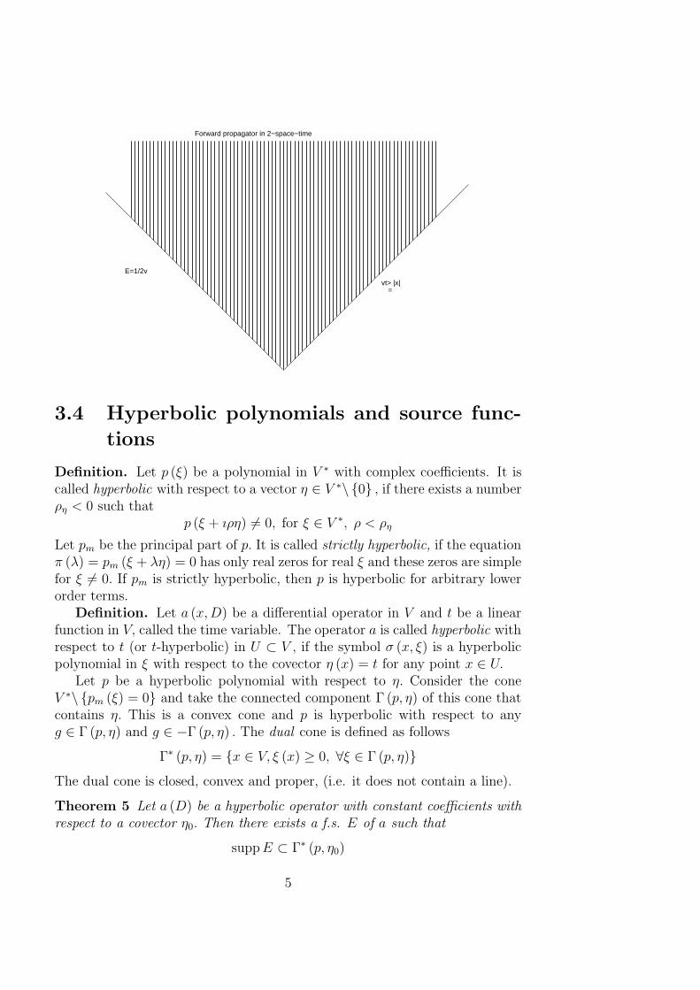
Example 6. For D’Alembert operator a (D) = ¤2.= ∂2t − v2∂2x we can
find a fundamental solution by means of the coordinate change y = x − vt,z = x + vt (see Ch.2): ¤2 = −4v2∂y∂z. Introduce the function (Heaviside’sfunction)
θ (x) = 1, for x ≥ 0, θ (x) = 0 for x < 0
We have ∂xθ (±x) = ±δ0, hence we can take
E (y, z) =(4v2
)−1θ (−y) θ (z) (3.1)
Returning to the space-time coordinate we get
E (x, t) = (2v)−1 θ (vt− |x|)
i.e. E (x, t) = (2v)−1 if vt ≥ |x| and E (x, t) = 0 otherwise. The coefficient 2vappears because of E is a density, (or a distribution), not a function.
We can replace θ (−y) to −θ (y) and θ (z) to −θ (−z) in (1) and get threemore options for a f.s.
Example 7. Consider the first order operator a (D) =∑aj∂j, with
constant coefficients aj ∈ R and introduce the variables y1, ..., yn such thata (D) y1 = 1, a (D) yj = 0, j = 2, ..., n and det ∂y/∂x = 1. Then the general-ized function E (x) = θ (y1) δ0 (y2, ..., yn) is a fundamental solution for a.
Problem. To check this statement.
4
Forward propagator in 2−space−time
vt> |x| =
E=1/2v
3.4 Hyperbolic polynomials and source func-
tions
Definition. Let p (ξ) be a polynomial in V ∗ with complex coefficients. It iscalled hyperbolic with respect to a vector η ∈ V ∗\ 0 , if there exists a numberρη < 0 such that
p (ξ + ıρη) 6= 0, for ξ ∈ V ∗, ρ < ρη
Let pm be the principal part of p. It is called strictly hyperbolic, if the equationπ (λ) = pm (ξ + λη) = 0 has only real zeros for real ξ and these zeros are simplefor ξ 6= 0. If pm is strictly hyperbolic, then p is hyperbolic for arbitrary lowerorder terms.
Definition. Let a (x,D) be a differential operator in V and t be a linearfunction in V, called the time variable. The operator a is called hyperbolic withrespect to t (or t-hyperbolic) in U ⊂ V , if the symbol σ (x, ξ) is a hyperbolicpolynomial in ξ with respect to the covector η (x) = t for any point x ∈ U.
Let p be a hyperbolic polynomial with respect to η. Consider the coneV ∗\ pm (ξ) = 0 and take the connected component Γ (p, η) of this cone thatcontains η. This is a convex cone and p is hyperbolic with respect to anyg ∈ Γ (p, η) and g ∈ −Γ (p, η) . The dual cone is defined as follows
Γ∗ (p, η) = x ∈ V, ξ (x) ≥ 0, ∀ξ ∈ Γ (p, η)The dual cone is closed, convex and proper, (i.e. it does not contain a line).
Theorem 5 Let a (D) be a hyperbolic operator with constant coefficients withrespect to a covector η0. Then there exists a f.s. E of a such that
suppE ⊂ Γ∗ (p, η0)
5
where p is the principal symbol of a.
Proof. Fix a covector η ∈ Γ (a, η0) , |η| = 1 and set
E (x) = (2π)−n limε→0
Eρ,ε (x) (3.2)
Eρ,ε (x) =
∫
V ∗
exp (ı 〈ξ + ıρη, x〉) exp(−ε (ξ + ıρη)2
)
p (ξ + ıρη)dξ
where n = dimV and p is the symbol of a. The dominator p (ξ + ıρη) doesnot vanish as ξ ∈ V ∗, η ∈ Γ (p, η0) , ρ < ρη, since a is η0-hyperbolic. Theintegral converges at infinity since of the decreasing factor exp (−εξ2) andcommutes with any partial derivative. The integrand can be extended to Cn
as a meromorphic differential form
ω = p−1 (ζ) exp(ıζx− εζ2
)dζ
that is holomorphic in the cone V ∗ + ıΓ (a, η0) ⊂ Cn. The integral of ω doesnot depend on ρ in virtue of the Cauchy-Poincare theorem (the special case ofthe general Stokes theorem). Check that it is a fundamental solution:
a (D)Eε,ρ (x, t) = ı−m
∫
V ∗
p (ξ + ıρη) exp (ı 〈ξ + ıρη, x〉) exp(−ε (ξ + ıρη)2
)
p (ξ + ıρη)dξ
=
∫
V ∗
exp (ı 〈ξ + ıρη, x〉) exp(−ε (ξ + ıρη)2
)dξ
=
∫
V ∗
exp (ıξx) exp(−εξ2
)dξ
= (πε)−n/2 exp(− (4ε)−1
(|x|2
))→ (2π)n δ0 in S
′
For the third step we have applied again the Cauchy-Poincare theorem. Thisyields a (D)E = δ0. Estimate this integral in the halfspace 〈η, x〉 < 0 :
|Eε (x)| =∣∣∣∣∣
∫
V ∗
exp (ı 〈ξ, x〉) exp (−ρ 〈η, x〉) exp(−ε (ξ + ıρη)2
)
p (ξ + ıρη)dξ
∣∣∣∣∣
≤ exp (−ρ 〈η, x〉)∫
V ∗
exp (−εξ2) exp (ερ2η2)|p (ξ + ıρη)| dξ ≤ Cε−n/2 exp
(ερ2
)exp (−ρ 〈η, x〉)
for a constant C, since of |p (ξ + ıρη)| ≥ c0 > 0. We take ε = ρ−2;the right sideis then equal to O (ρn exp (−ρ 〈η, x〉)) . This quantity tends to zero as ρ→ −∞,since 〈η, x〉 < 0. Therefore E (x) = 0 in the half-space Hη
.= 〈η, x〉 < 0 .
Therefore E vanishes in the union of all half-spaces Hη, η ∈ Γ (p, η0) . Thecomplement to this union in V is just Γ∗ (p, η0) . This completes the proof. ¡
Proposition 6 Let W ⊂ V be a closed half-space such that the conormal η isnot a zero the symbol am. If u a solution to the equation a (D)u = 0 supportedby W, then u = 0.
6
Proof. Take a hyperplane H ⊂ V \W. The distribution U vanishes in aneighborhood ofH and by Holmgren uniqueness theorem (see Ch.4) it vanisheseverywhere.
Corollary 7 If a a hyperbolic operator with constant coefficients with respectto a covector η, then there exists only one fundamental solution supported bythe set 〈η, x〉 ≤ 0 .
3.5 Wave propagators
The wave operator
¤n.=
∂2
∂t2− v2∆x
in V = X × R with a positive velocity v = v (x) is hyperbolic with respect tothe time variable t. The symbol σ (ξ, τ) = −τ 2 + v2 |ξ|2 is strictly hyperbolicwith respect to the covector η0 = (0, 1) . Now we assume that the velocity vis constant; the wave operator is hyperbolic and with respect to any covector(η, 1) such that v |η| < 1 and the union of these covectors is just the coneΓ (σ, η0) . The dual cone is
Γ∗ (σ, η0) = (x, t) , v |x| ≥ t
The f.s. supported by this cone is called the forward propagator. For theopposite cone −Γ∗ = v |x| ≤ t the corresponding f.s. is called the backwardpropagator. Both fundamental solutions are uniquely defined.
For the case dimV = 2 both propagators were constructed in Example 6in the previous section.
Proposition 8 The forward propagator for ¤4 is
E4 (x, t) =1
4πv2tδ (|x| − vt) (3.3)
This f.s. acts on test functions φ ∈ D (V )as follows
E4 (φ) =(4πv2
)−1∫ ∞
0
t−1∫
|x|=vt
φ (x, t) dSdt
Proof. Write (2) for the vector η0 = (0,−1) in the form
E (x, t) = (2π)−4 limε→0
Eε (x, t) (3.4)
Eε (x, t) = −∫
X∗
∫ ∞
−∞
exp (ıξx+ ı (τ − ıρ) t) exp (−εξ2)(τ − ıρ)2 − |vξ|2
dτdξ
7
where ξ, τ are coordinates dual to x, t, respectively and we write ξx insteadof 〈ξ, x〉 . The interior integral converges, hence we need not the decreasingfactor exp (−ετ 2) . We know that E vanishes for t < 0; assume that t > 0. Thebackward propagator vanishes, hence we can take the difference as follows:
Eε (x, t) = −∫
X∗
exp(−εξ2
)dξ×
∫ ∞
−∞
[exp (ıξx+ ı (τ − ıρ) t)
(τ − ıρ)2 − |vξ|2− exp (ıξx+ ı (τ + ıρ) t)
(τ + ıρ)2 − |vξ|2]dτ
The interior integral is equal to the integral of the meromorphic form ω =(ζ2 − |vξ|2
)−1exp (ı 〈ξ, x〉+ ıζt) over the chain Im ζ = −ρ−Im ζ = ρ , which
is equivalent to the union of circles |ζ − |vξ|| = ρ ∪ |ζ + |vξ|| = ρ . By theresidue theorem we find∫...dτ = 2πı exp (ıξx)
exp (ıvt |ξ|)− exp (−ıvt |ξ|)2v |ξ| = −2π exp (ıξx) sin (vt |ξ|)
v |ξ|consequently
Eε (x, t) = 2πv−1∫
X∗
exp (ıξx)sin (vt |ξ|)
|ξ| exp(−εξ2
)dξ
= 2πv−1F ∗
(sin (vt |ξ|)
|ξ| exp(−εξ2
))
Lemma 9 We have for an arbitrary a > 0
F(δS(a)
)= 4πa
sin (a |ξ|)|ξ| (3.5)
where δS(a) denotes the delta-density on the sphere S (a) of radius a :
δS(a) (φ) =
∫
S(a)
φdS
Proof of Lemma. For an arbitrary test function ψ ∈ D (X∗) we have
F(δS(a)
)(ψ) = δS(a) (F (ψ)) = δS(a)
(∫exp (−ıxξ)ψ (ξ) dξ
)
=
∫ψ (ξ) δS(a) (exp (−ıxξ)) dξ
The functional δS(a) has compact support and therefore is well defined on thesmooth function exp (−ıxξ) . Calculate the value:
δS(a) (exp (−ıxξ)) =∫
S(a)
exp (−ıxξ) dS = a2∫ 2π
0
∫ π
0
exp (−ıa |ξ| cos θ) sin θdθdϕ
= −2πıa2 exp (ıa |ξ|)− exp (−ıa |ξ|)a |ξ| = 4πa
sin (a |ξ|)|ξ|
8
This implies (5).
We have F ∗F = (2π)3 I, where I stands for the identity operator, henceby (4)
F ∗
(sin (a |ξ|)|ξ|
)= 2π2a−1δS(a)
We find from (5)
Eε (x, t) = 2πv−1F ∗
(sin (vt |ξ|)
|ξ| exp(−εξ2
))→ 4π3v−2t−1δS(vt)
This implies (3) in virtue of (4). ¤
Problem. Calculate the backward propagator for ¤4.
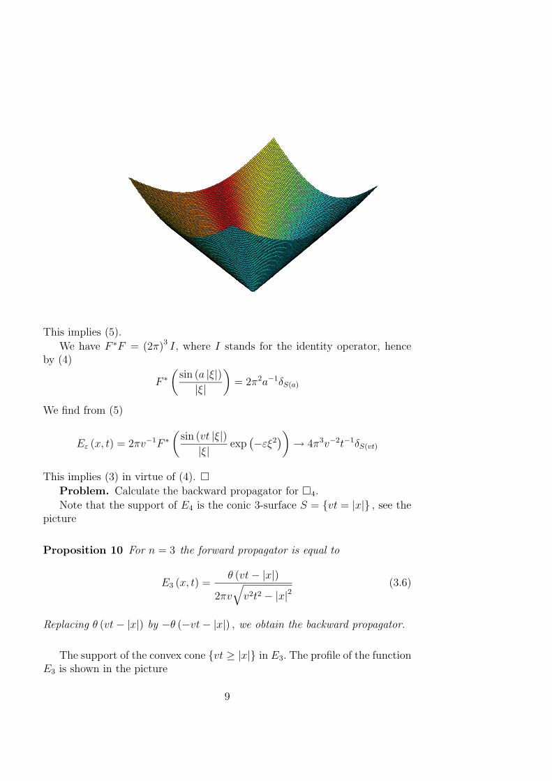
Note that the support of E4 is the conic 3-surface S = vt = |x| , see thepicture
Proposition 10 For n = 3 the forward propagator is equal to
E3 (x, t) =θ (vt− |x|)
2πv√v2t2 − |x|2
(3.6)
Replacing θ (vt− |x|) by −θ (−vt− |x|) , we obtain the backward propagator.
The support of the convex cone vt ≥ |x| in E3. The profile of the functionE3 is shown in the picture
9
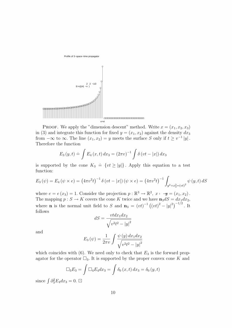
Profile of 3−space−time propagator
x=vt
E=c((vt) −x ) 2 2 −1/2
Proof. We apply the ”dimension descent” method. Write x = (x1, x2, x3)in (3) and integrate this function for fixed y = (x1, x2) against the density dx3from −∞ to ∞. The line (x1, x2) = y meets the surface S only if t ≥ v−1 |y| .Therefore the function
E3 (y, t).=
∫E4 (x, t) dx3 = (2πv)−1
∫δ (vt− |x|) dx3
is supported by the cone K3.= vt ≥ |y| . Apply this equation to a test
function:
E3 (ψ) = E4 (ψ × e) =(4πv2t
)−1δ (vt− |x|) (ψ × e) =
(4πv2t
)−1∫
y2+x2
3=(vt)2
ψ (y, t) dS
where e = e (x3) = 1. Consider the projection p : R3 → R2, x 7→y = (x1, x2) .The mapping p : S → K covers the cone K twice and we have n3dS = dx1dx2,
where n is the normal unit field to S and n3 = (vt)−1((vt)2 − |y|2
)−1/2. It
follows
dS =vtdx1dx2√v2t2 − |y|2
and
E3 (ψ) =1
2πv
∫ψ (y) dx1dx2√v2t2 − |y|2
which coincides with (6). We need only to check that E3 is the forward prop-agator for the operator ¤3. It is supported by the proper convex cone K and
¤3E3 =
∫¤4E4dx3 =
∫δ0 (x, t) dx3 = δ0 (y, t)
since∫∂23E4dx3 = 0. ¡
10
3.6 Inhomogeneous hyperbolic operators
Example 7. The forward propagator for the Klein-Gordon-Fock operator¤4 +m2 is equal to
D (x, t) =θ (t)
4πc2tδ (ct− |x|)− m
4πθ (ct− |x|)
J1
(m√c2t2 − |x|2
)
√c2t2 − |x|2
(3.7)
where J1 is a Bessel function. Recall that the Bessel function of order ν canbe given by the formula
Jν (z) =∞∑
0
(−1)kk!Γ (ν + k + 1)
(z2
)ν+2k
Remark. The generalized functions in (3), (6), and (7) can be written aspullbacks of some functions under the mapping
X × R → R2, (x, t)→ q = v2t2 − |x|2 , θ (t) (3.8)
It is obvious for (6) since θ (vt− |x|) = θ (q) θ (t) . Fix the coordinates (x0, x)in V, where x0 = vt. In formulae (3) and (7) we can write (ct)−1 δ (ct− |x|) =δ (q) . Indeed, we have by definition
δ (q) (α) =
∫
q=0
α
dq=√1 + v2
∫ ∞
0
∫
q=0
φ
|∇q|dSdt
where α = φdxdx0 is a test density, i.e. φ ∈ D (X × R); dS is the areain the 2-surface q = 0, t = const . We have ∇q = (2x, 2v2t) = (2x, 2v2t) ,|∇q| = 2
√1 + v2vt and
∫
q=0
φ
|∇q|dS =(2√1 + v2vt
)−1∫φdS
Then
E4 =θ (t)
4πv2tδ (|x| − vt) =
θ (t)
2πvδ (q)
D = θ (t)
[1
2πcδ (q)− m
4πθ (q)
J1(m√q)
√q
]
This fact has the following explanation. The wave operator and the Klein-Gordon-Fock operator are invariant with respect to the Lorentz group L3 =O (3, 1) . This is the group of linear transformations in V that preserve thequadratic form q; the dual transformations in V ∗ preserve the dual form
11
q∗ (ξ, τ) = τ 2− c2 |ξ|2 . Any Lorentz transformation preserves the volume formdV = dxdt too. Therefore the variety of all source functions is invariant withrespect to this group. The forward propagator is uniquely define. Therefore itis invariant with respect to the orthochronic Lorentz group L3↑, i.e. to group oftransformations A ∈ L3 that preserves the time direction. The functions q andsgn t are invariant of the orthochronic Lorentz group and any other invariantfunction (even a generalized function) is a function of these two. We see thatis the fact for the forward propagators (as well as for backward propagators).
Example 8. The function
Dc (x, t).= − (2π)−4
∫
X∗
∫
R∗
exp (ıτ t+ ı (ξ, x)) dτdξ
τ 2 − ξ2 + εı
is also a fundamental solution for the wave operator ¤4. The integral mustbe regularized at infinity by introducing a factor like exp (−ε′ξ2) ; it does notdepend on ε > 0 since the dominator has no zeros in V ∗ = X∗ × R∗. Thisfunction is called causal propagator and plays fundamental role in the tech-niques of Feynman diagrams ? It is invariant with respect to the completeLorentz group L3. The causal propagator vanishes in no open set, hence it isnot equal to a linear combination of the forward and backward propagators.The causal propagator for the Klein-Gordon-Fock operator is defined in by thesame formula with the extra term m2 in the dominator.
3.7 Riesz groups
This construction provides an elegant and uniform method for explicit con-struction of forward propagators for powers of the wave operator in arbitraryspace dimension.
Let V be a space of dimension n with the coordinates (x1, ..., xn); set q (x) =x21 − x22 − ...− x2n. The set K
.= x1 ≥ 0, q (x) ≥ 0 is a proper convex cone in
V. Consider the family of distributions
qλ+ (φ) =
∫
K
qλ (x)φ (x) dx, φ ∈ D (V ) , λ ∈ C
This family is well-defined in the halfplane Reλ > 0 and is analytic, i.e.qλ+ (φ) is an analytic function of λ for any φ. The family has a meromorphiccontinuation to whole plane C with poles at the points
λ = 0,−1,−2, ...; λ =n
2− 1,
n
2− 2, ...
and after normalization
Zλ.=
qλ−n/2+ dx
π(n−2)/222λ−1Γ (λ) Γ (λ+ 1− n/2),xλ−1+ dx
Γ (λ)(3.9)
12
becomes an entire function of λ with values in the space of tempered distri-butions. We have always suppZλ ⊂ K, hence Zλ is an element of the algebraAK of tempered distributions with support in the convex closed cone K. Theconvolution is well-defined in this algebra; it is associative and commutative.The following important formula is due to Marcel Riesz :
Zλ ∗ Zµ = Zλ+µ (3.10)
The points λ = 0,−1,−2, ... are poles of the numerator and denominator in(9) and the value of Zλ at these points can be found as a ratio of residues:
Z0 = δ0dx, Z−k = ¤kZ0 (3.11)
where ¤ = ∂21 − ∂22 − ...− ∂2n is the differential operator dual to the quadraticform q. In particular, the convolution φ 7→Z0 ∗ φ is the identity operator; thistogether with (10) means that the family of convolution operators Zλ∗ is acommutative group, which is isomorphic to the additive group of C. It is calledthe Riesz group. From (11) we see that
¤kZk = Z−k ∗ Zk = Z0 = δ0dx
This means that Zk is a fundamental solution for the hyperbolic operator¤
k (which is not strictly hyperbolic for k > 1). Moreover it is a forwardpropagator, since suppZk ⊂ K.
If the dimension n is even, the point λ = k = n/2− 1 is again a pole of thenumerator and denominator in (9), as a consequence of which the support ofZk is contained in the boundary ∂K. This fact is an expression of the strongHuyghens principle: for even dimension the wave initiated by a local sourcehas back front, whereas the forward front exists for arbitrary dimension. Thisis just the case for n = 4, k = 1.
References
[1] L.Schwartz: Theorie des distributions (Theory of distributions)[2] R.Courant, D.Hilbert: Methods of Mathematical Physics[3] I.Rubinstein, L.Rubinstein: Partial differential equations in classical
mathematical physics[4] F.Treves: Basic linear partial differential equations[5] V.S.Vladimirov: Equations of mathematical physics
13
Chapter 4
The Cauchy problem
4.1 Definitions
Let a (x,D) be a linear differential operator of order m with smooth coefficients in thespace V n and W be an open set in V. Let t be a smooth function in W such thatdt 6= 0 (called time variable) and f, g be some functions in W. The Cauchy problem for”time” variable t for the data f, g is to find a solution u to the equation
a (x,D) u = f (4.1)
in W that fulfils the initial condition
u− g = O (tm)
in a neighborhood of W0.= x ∈ W, t (x) = 0 .
First, assume that the right-hand side f and g are smooth. Introduce the coordinatesx′ = (x1, ..., xn−1) (space variables) such that (x
′, t) is a coordinate system in V. Writethe equation in the form
a (x,D) u = α0∂mt u+ α1∂
m−1t u+ ...+ αmu = f (4.2)
where αj, j = 0, 1, ...,m is a differential operator of order ≤ j which does not containtime derivatives. In particular, α0 is a function. The initial condition can be written inthe form
u|t=0 = g0, ∂tu|t=0 = g1, ..., ∂m−1t u|t=0 = gm−1
where gj = ∂jt g|t=0, j = 0, ...,m− 1 are known functions in W0. Set t = 0 in (2) and find
α0∂mt u|t=0 =
(f − α1∂
m−1t u− ...− αmu
)|t=0 = f |t=0 − α1gm−1 − ...− αmg0
from this equation we can find the function ∂mt u|W0, if α0|W0 6= 0. Take t-derivative ofboth sides of (2) and apply the above arguments to determine ∂m+1
t u|W0 and so on.Definition. The hypersurface W0 is called non-characteristic for the operator a at
a point x ∈ W0, if α0 (x) 6= 0. Note that α0 (x) = σm (x, dt (x)) , where σm|W × V ∗ is theprincipal symbol of a and η ∈ V ∗, η (x) = t. An arbitrary smooth hypersurface H ⊂ V
1
is non-characteristic at a point x, if σm (x, η) 6= 0, where η is the conormal vector to Hat x.The necessary condition for solvability of the Cauchy for arbitrary data is that the
hypersurfaceW0 is everywhere non-characteristic. This condition is not sufficient. For el-liptic operator a an arbitrary hypersurface is non-characteristic, but the Cauchy problemcan be solved only for a narrow class of initial functions g0, ..., gm−1.
Example 1. For the equation∂2u
∂t∂x= 0
the variable t as well as x is characteristic, n = 2; σ2 = τξ. dt = (0, 1) ;σ2 (0, 1) = 0.Example 2. For the heat equation
∂tu−∆x′u = 0
the variable t is characteristic, but the space variables are not. u|t = 0 = u0.
Example 3. The Poisson equation ∆u = 0 is elliptic, but the Cauchy problem
u|W0 = g0, ∂tu|W0 = g1
has no solution in W , unless g0 and g1 are analytic functions. In fact, it has no solutionin the half-space W+, if g0, g1 are in L2 (W0), unless these functions satisfy a strongconsistency condition.
4.2 Cauchy problem for distributions
The non-characteristic Cauchy problem can be applied to generalized functions as well.First, we write our space as the direct product V = X×R by means of coordinates x′ andt. For arbitrary test densities ψ and ρ in X and R, respectively, we can take the productφ (x′, t) = ψ (x′) ρ (t) . It is a test density in V. Let now u an arbitrary (generalized)function in V , fix ψ and define the function in R by
uψ (ρ) = u (ψρ) =
∫vψρ, vψ ∈ C
∞
Definition. The function u is called weakly smooth in t-variable (or t-smooth), if thefunctional uψ coincides with a smooth function for arbitrary ψ ∈ D (X) .Any smooth function is obviously weakly smooth in any variable. A weaker sufficient
condition can be done in terms of the wave front of u.If u is weakly smooth in t, then ∂tu is also weakly smooth in t and the restriction
operator u 7→u|t=τ is well defined for arbitrary τ :
u|t=τ (ψ) = limk→∞
u (ψρk)
where ρk ∈ D (R) is an arbitrary sequence of densities that weakly tends to the delta-distribution δτ . The limit exists, because of the assumption on u.
2
010
2030
4050
6070
0
20
40
60
80−8
−6
−4
−2
0
2
4
6
8
Theorem 1 Suppose that the operator a with smooth coefficients is non-characteristic in
t. Any generalized function u that satisfies the equation a (x,D) u = 0 is weakly smoothin t variable. The same is true for any solution of the equation a (x,D) u = f, where f
is an arbitrary weakly t-smooth function.
It follows that for any solution of the above equation the initial data ∂jtu|t=0 are welldefined, hence the initial conditions (2) is meaningful.Now we formulate the generalized version of the Holmgren uniqueness theorem:
Theorem 2 Let a (x,D) be an operator with real analytic coefficients, H is a non-
characteristic hypersurface. There exists an open neighborhood W of H in V such that
any function that satisfies of a (x,D) u = 0 in W that fulfils zero initial conditions in H,
vanishes in W.
4.3 Hyperbolic Cauchy problem
Theorem 3 Suppose that the operator a with constant coefficients is t-hyperbolic. Then
for arbitrary generalized functions g0, ..., gm−1 in W0 = t = 0 and arbitrary functionf ∈ D ′ (V ) that is weakly smooth in t, there exists a unique solution of the t-Cauchyproblem.
Proof. The uniqueness follows from the Holmgren theorem. Choose linear functionsx = (x1, ..., xn−1) such that (x, t) is a coordinate system.
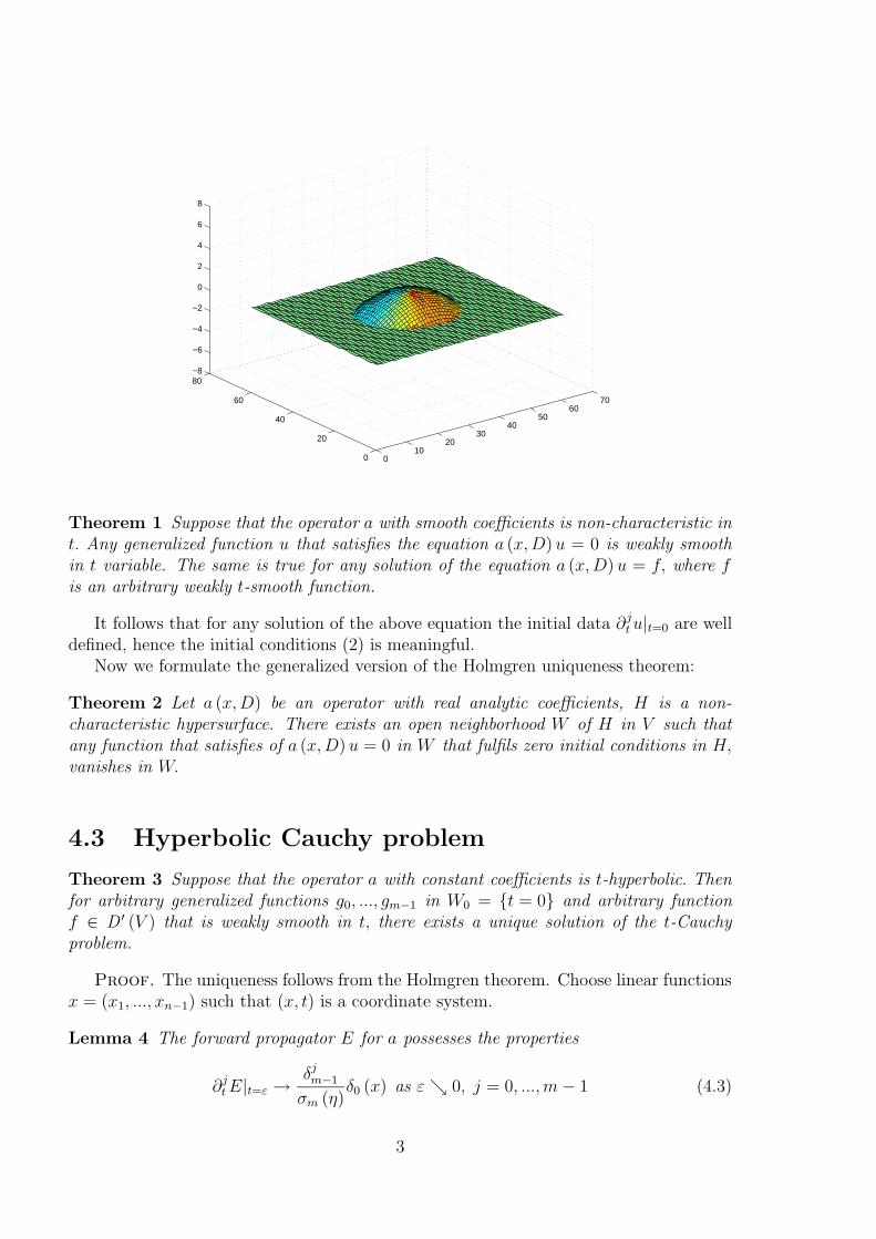
Lemma 4 The forward propagator E for a possesses the properties
∂jtE|t=ε →
δjm−1
σm (η)δ0 (x) as ε 0, j = 0, ...,m− 1 (4.3)
3
Proof of Lemma. Apply the formula (2) of Ch.3
E (x, t) = (2π)−n limε→0
Eρ,ε (x, t)
Eρ,ε (x, t) =
∫
X∗
∫ ∞
−∞
exp ((ıτ + ρ) t)
a (ıξ, ıτ + ρ)dτ exp
(ıξx− ε |ξ|2
)dξ, ρ < ρη
We use here the notation V ∗ = X∗ × R and the corresponding coordinates (ξ, τ) . Weassume that m ≥ 2, therefore the interior integral converges without the auxiliary de-creasing factor exp (−ετ 2) . We can write the interior integral as follows
−ı
∫
γ
exp (ζt) dζ
a (ıξ, ζ)
where γ = Re ζ = ρ . All the zeros of the dominator are to the left of γ. By CauchyTheorem we can replace γ by a big circle γ ′ that contains all the zeros, since the numeratoris bounded in the halfplane Re ζ < ρ . The integral over γ ′ is equal to the residue of theform ω = a−1 (ıξ, ζ) exp (ζt) dζ at infinity times the factor (2πı)−1
. The residue tends tothe residue of the form a−1 (ıξ, ζ) dζ as t→ 0. The later is equal to zero since order of ais greater 1. This implies (4) for j = 0. Taking the j-th derivative of the propagator, wecome to the form ζja−1 (ıξ, ζ) dζ. Its residue at infinity vanishes as far as j < m− 1. Inthe case j = m−1 the residue at infinity is equal to α−1
0 , where α0 is as in (3). Thereforethe m− 1-th time derivative of the interior integral tends to 2πα−1
0 , hence
∂m−1t Eρ,ε (x, t)→ 2πα−1
0
∫
X∗
exp (ıξx) dξ = (2π)n−1α−1
0 δ0 (x)
Taking in account that α0 = am (η) , we complete the proof. ¡Note that for any higher derivative ∂jtE the limit as (4) exists and can be found from
(4) and the equation a (D)E = 0 for t > 0.Proof of Theorem. First we define a solution u of (1) by
u = E ∗ f
The convolution is well defined, since supp f ⊂ H+ and suppE ⊂ K, the cone K isconvex and proper. The distribution u is weakly smooth in t, hence the initial data of itare well defined. Therefore we need now to solve the Cauchy problem for the equation
a (D) u = 0 (4.4)
with the initial conditions
u|t=0 = g0, ∂ηu|t=0 = g1, ..., ∂m−1u|t=0 = gm−1 (4.5)
where gj = uj − ∂jt u|t=0, j = 0, ...,m− 1. Take first the convolution
e0.= α0
(∂m−1t E ∗ g0
)(t, x) = α0
∫∂m−1t E (t, x− y) g0 (y) dy (4.6)
This is a solution of (5); according to Lemma and e0|t=0 = g0. The derivatives ∂jt e0|t=0
can be calculated by differentiating (7), since any time derivative of E has a limit as
4
t→ 0. Therefore we can replace the unknown function u by u′.= u− e0. The function u
′
must satisfies the conditions like (6) with g0 = 0. Then we take the convolution
e1.= α0
(∂m−2t E ∗ g1
)
By Lemma we have e1|t=0 = 0 and ∂te1|t=0 = g1. Then we replace u′ by u′′ = u′ − e1 and
so on. ¡
4.4 Solution of the Cauchy problem for wave equa-
tions
Applying the above Theorem to the wave equations with the velocity v, we get theclassical formulae:
Case n = 2. The D’Alembert formula
2vu (x, t) =
∫ t
0
∫ x+v(t−s)
x−v(t−s)
f (y, s) dyds
+
∫ x+vt
x−vt
g1 (y) dy + v [g0 (x+ vt) + g0 (x− vt)]
Case n = 3. The Poisson formula
2πvu (x, t) =
∫ t
0
∫
B(x,v(t−s))
f (y, s) dyds√v2 (t− s)2 − |x− y|2
+
∫
B(x,vt)
g1 (y) dy√v2t2 − |x− y|2
+ ∂t
∫
B(x,vt)
g0 (y) dy√v2t2 − |x− y|2
Case n = 4. The Kirchhof formula
4πv2u (x, t) =
∫
B(x,vt)
f (y, t− v−1 |x− y|) dy
|x− y|
+
∫
S(x,vt)
g1 (y) dS + ∂t
(t−1
∫
S(x,vt)
g0 (y) dS
)
Here B (x, r) denotes the ball with center x, radius r; S (x, r) is the boundary of this ball.
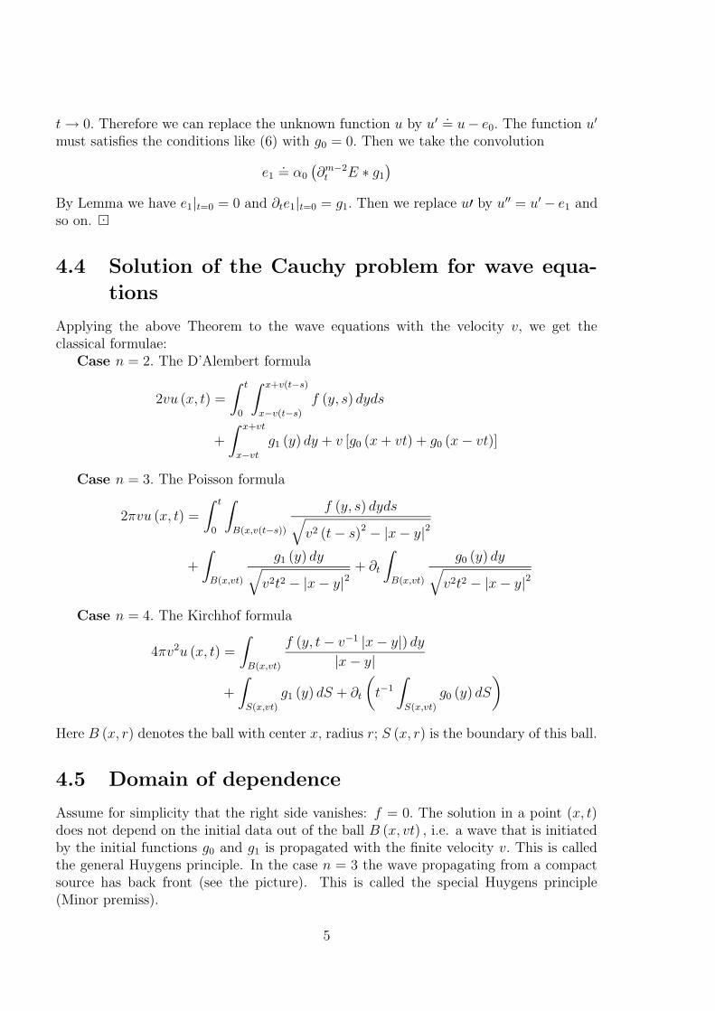
4.5 Domain of dependence
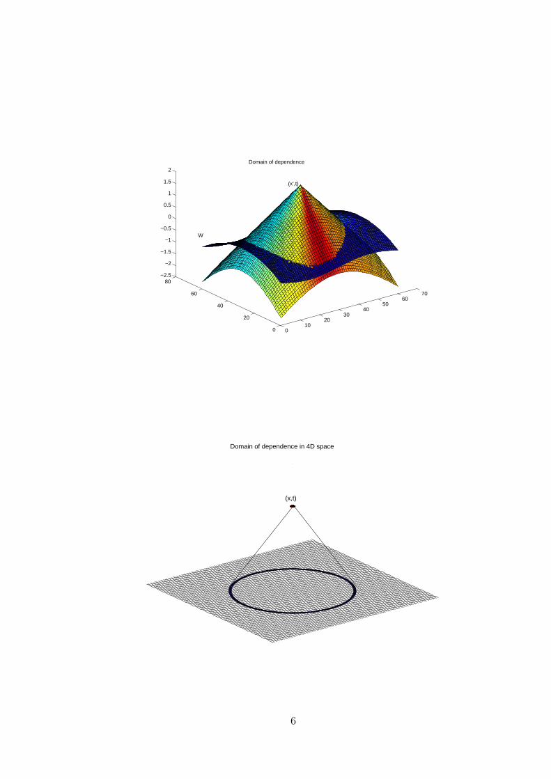
Assume for simplicity that the right side vanishes: f = 0. The solution in a point (x, t)does not depend on the initial data out of the ball B (x, vt) , i.e. a wave that is initiatedby the initial functions g0 and g1 is propagated with the finite velocity v. This is calledthe general Huygens principle. In the case n = 3 the wave propagating from a compactsource has back front (see the picture). This is called the special Huygens principle(Minor premiss).
5
010
2030
4050
6070
0
20
40
60
80−2.5
−2
−1.5
−1
−0.5
0
0.5
1
1.5
2
Domain of dependence
(x’,t)
W
Domain of dependence in 4D space
(x,t)
6
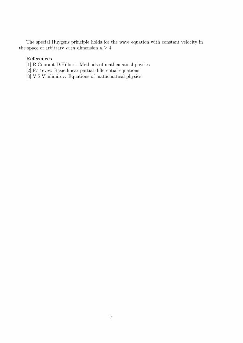
The special Huygens principle holds for the wave equation with constant velocity inthe space of arbitrary even dimension n ≥ 4.
References
[1] R.Courant D.Hilbert: Methods of mathematical physics[2] F.Treves: Basic linear partial differential equations[3] V.S.Vladimirov: Equations of mathematical physics
7
Chapter 5
Helmholtz equation and
scattering
5.1 Time-harmonic waves
Let a (x,Dx, Dt) be a linear differential operator of order m with smooth coeffi-cients in the space-time V = Xn × R with coordinates (x, t) , whose coefficientsdo not depend on the time variable t. Consider the equation
a (x,Dx, Dt)U (x, t) = F (x, t) (5.1)
A function of the form F (x, t) = exp (ıωt) f (x) is called time-harmonic of fre-quency ω, the function f is called the amplitude. If a solution is also time-harmonic function U (x, t) = exp (ıωt)u (x), we obtain the time-independentequation for the amplitudes
a (x,Dx, ıω)u (x) = f (x)
Example 1. For the Laplace operator in space-time a (Dx, Dt) = D2t + ∆X we
havea (Dx, ıω) = −ω2 +∆
This is a negative operator. Therefore any solutions of the equation (ω2 −∆)u =0 in X of finite energy i.e. u ∈ L2 (X) decreases fast at infinity.Example 2. If a = D2
t − v2 (x)∆ is the wave operator and the velocity v doesnot depend on time, then
−a (x,Dx, ıω) = ω2 + v2 (x)∆
is the Helmholtz operator. The Helmholtz equation with f = 0 is usually writtenin the form (
∆+ n2ω2)u = 0
where the function n.= v−1 is called the refraction coefficient. The Helmholtz
operator is not definite; there are many oscillating bounded solutions of the formu (x) = exp (ıξx) , where σ
.= n2ω2− ξ2 = 0, ξ ∈ Rn. This solution is unbounded,
when ξ ∈ Cn\Rn.Find a fundamental solution for the time-independent equation:
1
Proposition 1 Let E (x, t) be a fundamental solution for (1) that can be repre-sented by means of the Fourier integral
Ey (x, t) =1
2π
∫exp (ıωt) Ey (x, ω) dω (5.2)
for a tempered (Schwartz) distribution E. Then
a (x,Dx, ıω) Ey (x, ω) = δy (x) (5.3)
i.e. E (x, ω) is a source function for the operator a (x,Dx, ıω) for any ω such thatE is weakly ω-smooth.
Proof. We have
δy (x, t) = a (x,Dx, Dt)Ey (x, t) =1
2π
∫exp (ıωt) a (x,Dx, ıω) Ey (X,ω) dω
At the other hand
δ0 (t) =1
2π
∫exp (ıωt) dω, δy (x, t) = δ (t) δy (x) =
1
2π
∫exp (ıωt) dωδy (x)
Comparing, we get
∫exp (ıωt) a (x,Dx, ıω) E (x, ω) dω =
∫exp (ıωt) dωδ (x)
which implies (3) in the sense of generalized functions in V ×R∗. If Ey (x, ω) is ω-smooth for some ω0 we can consider the restriction of both sides to the hyperplaneω = ω0. Then we obtain (3).
5.2 Source functions for Helmholtz equation
Apply this method to the wave operator with a constant velocity v. Take theforward propagator E. It is supported in t ≥ n |x| and bounded as t → ∞.Therefore it can be represented by means of the Fourier integral (2) for thetempered distribution
E (x, ω) =
∫ ∞
n|x|
E (x, t) exp (−ıωt) dt (5.4)
The corresponding source function for the Helmholtz operator is equal Fn (x, ω).=
−v2En+1 (x,−ω) . Calculate it:Case n = 1. We have E2 (x, t) = (2v)
−1 θ (vt− |x|) and
F1 (x, ω) = −∫ ∞
n|x|
exp (ıωt) dt =−ı2ωn
exp (ıωn |x|)
2
Case n = 3. We have
F3 (x, ω) = −1
4πn |x|
∫ ∞
0
δ (|x| − vt) exp (ıωt) dt = −exp (ıωn |x|)4π |x|
Case n = 2. We have
F2 (x, ω) =1
2π
∫ ∞
n|x|
exp (ıωt)√t2 − n2 |x|2
dt
This integral is not an elementary function; it is equal to c0H(1)0 (ωn |x|) , where
H(1)0 is a Hankel function. The equation F2 (x) = − (2π)−1 ln |x|+R (x, ω) , where
R is a C1-function in a neighbourhood of the origin.
Proposition 2 The function Fn (x, ω) is the boundary value at the ray ω > 0of a function Fn (x, ζ) that is holomorphic in the half-plane ζ = ω + ıτ, τ > 0 .
Proof. The integral (4) has holomorphic continuation at the opposite half-plane.
5.3 Radiation condition
Let K be a compact set in X3 with smooth boundary and connected complementX\K. Consider the exterior boundary problem
(∆+ k2
)u (x) = 0, x ∈ X\K, k = ωn (5.5)
u (x) = f (x) , x ∈ ∂K (Dirichlet condition)
where f is a function on the boundary. Any solution is a real analytic functionu = u (x) since the Helmholtz operator is of elliptic type. A solution is notunique, unless an additional condition is imposed. The radiation (Sommerfeld)condition is as follows
ur − ıku = o(r−1
)as r = |x| → ∞; ur = ∂u/∂r (5.6)
Theorem 3 If k > 0 and f = 0, there is only trivial solution u = 0 to theexterior problem satisfying the radiation condition.
Proof. Let S (R) denote the sphere |x| = R in X.We have S (R) ⊂ X\Kfor large R ≥ R0. Write for an arbitrary solution u :∫
S(R)
|ur − ıku|2 dS =∫
S(R)
(|ur|2 + k2 |u|2
)dS − ık
∫
S(R)
(uru− uur) dS (5.7)
By (6) the left side tends to zero as R → ∞. At the other hand, by Green’sformula ∫
S(R)
(uru− uur) dS =
∫
∂K
(∂νuu− u∂νu) dS
3
where ∂ν stands for the normal derivative on ∂K. The right side vanishes, sinceu|∂K = 0, hence (7) implies
∫
S(R)
|u|2 dS → 0, R→∞ (5.8)
Lemma 4 [Rellich] For k > 0 any solution u of the Helmholtz equation in X\Ksatisfying (8) equals identically zero.
Proof. Consider the integral
U (r).=
∫
S2
u (rs)φ (s) ds
where φ is a continuous function and ds is the Euclidean area density in the unitsphere S2. We prove that U (r) = 0 for r > R0 and for each eigenfunction φ ofthe spherical Laplace operator ∆S:
∆Sφ = λφ
R (λ).= (∆S − λId)−1 . In view of the formula
∆ = ∂2r + 2r
−1∂r + r−2∆S
it follows that U (r) satisfies the ordinary equation
Urr + 2r−1Ur +
(k2 + λr−2
)U = 0, r > R0
This differential equation has two solutions of the form
U± (r) = C±r−1 exp (±ıkr) + o
(r−1
), r →∞
Clearly, no nontrivial linear combination of U+ and U− is o (r−1) . A the other
hand the hypothesis implies that U (r) = o (r−1) ; we deduce that U = 0. Theoperator ∆S is self-adjoint non-positive and the resolvent is compact. The set ofeigenfunctions is a complete system in L2 (S
2) by Hilbert’s theorem. This impliesthat u = 0 for |x| > R0. The function u is real analytic, consequently it vanisheseverywhere in X\K. ¤Now we state existence of a solution of the problem (5).
Theorem 5 [Kirchhof-Helmholtz] If the function f is sufficiently smooth, thenthere exists a solution of (5) satisfying the radiation condition. This solution isof the form
u (x) =
∫
∂K
[f (y) ∂ν
exp (ık |x− y|)|x− y| − g (y)
exp (ık |x− y|)|x− y|
]dSy, g = ∂νu
(5.9)
4
Sketch of a proof. First we replace the Helmholtz operator by ∆ +(k + ıε)2 . The function F3 (x, k + εı)
.= − (4π |x|)−1 exp ((ık − ε) |x|) is a funda-
mental solution which coincides with F3 (x, k) for ε = 0. The symbol equalsσε = − |ξ|2+(k + εı)2 and |σε| ≥ ε2 > 0. Therefore there exists a unique functionuε ∈ L2 (X\K) that satisfies the conditions
(∆+ (k + ıε)2
)uε = 0 in X\K
uε|∂K = f
(This fact follows from standard estimates for solutions of a elliptic boundaryvalue problem.) Moreover the sequence uε has a limit u in X\K and on ∂K asε → 0 and ∂νuε → ∂νu. This is called limiting absorption principle. By Green’sformula
uε (x) =
∫
∂K
−∫
S(R)
[f (y) ∂ν
exp ((ık − ε) |x− y|)|x− y| − g (y)
exp ((ık − ε) |x− y|)|x− y|
]dSy
for x ∈ B (R) \K, where B (R) is the ball of radius R. Take R→∞; the integralover S (R) tends to zero, hence it can be omitted in this formula. Passing to thelimit as ε → 0, we get (9). It is easy to see that right side of (9) satisfies theradiation condition. Indeed, we have for any y ∈ ∂K the kernel in the secondterm (simple layer potential) fulfils this condition, since
∂rexp (ık |x− y|)
|x− y| =
(x
|x| ,∇)exp (ık |x− y|)
|x− y|
=(x, x− y)
|x| |x− y|ık exp (ık |x− y|)
|x− y| +O(|x|−2)
=ık exp (ık |x− y|)
|x− y| +O(|x|−2)
The kernel in the first term (double-layer) equals
∂νexp ((ık − ε) |x− y|)
|x− y| =(ν, x− y)
|x− y|exp (ık |x− y|)
|x− y| +O(|x|−2)
and fulfils this condition too. ¤The equation (9) is called the Kirchhof representation. The functions f, g are
not arbitrary, in fact, g = Λf, where Λ is a first order pseudodifferential operatoron the boundary.
Exercise. Check the formula ∆S = (sin θ)−1 ∂θ sin θ∂θ + sin
2 θ∂2φ.
Problem. Show that the operator ∆S is self-adjoint non-positive and theresolvent is compact.
Remark. The radiation condition is a method to single out a unique solutionof the exterior problem. The real part of this solution is physically relevant, inparticular,
<F3 =cos (k |x|)4π |x|
is also a source function. Therefore we can replace ı to −ı simultaneously in (4),(6) and (9).
5
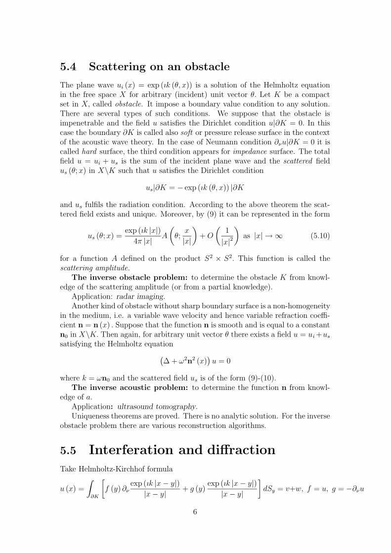
5.4 Scattering on an obstacle
The plane wave ui (x) = exp (ık (θ, x)) is a solution of the Helmholtz equationin the free space X for arbitrary (incident) unit vector θ. Let K be a compactset in X, called obstacle. It impose a boundary value condition to any solution.There are several types of such conditions. We suppose that the obstacle isimpenetrable and the field u satisfies the Dirichlet condition u|∂K = 0. In thiscase the boundary ∂K is called also soft or pressure release surface in the contextof the acoustic wave theory. In the case of Neumann condition ∂νu|∂K = 0 it iscalled hard surface, the third condition appears for impedance surface. The totalfield u = ui + us is the sum of the incident plane wave and the scattered fieldus (θ;x) in X\K such that u satisfies the Dirichlet condition
us|∂K = − exp (ık (θ, x)) |∂K
and us fulfils the radiation condition. According to the above theorem the scat-tered field exists and unique. Moreover, by (9) it can be represented in the form
us (θ;x) =exp (ık |x|)4π |x| A
(θ;
x
|x|
)+O
(1
|x|2)as |x| → ∞ (5.10)
for a function A defined on the product S2 × S2. This function is called thescattering amplitude.
The inverse obstacle problem: to determine the obstacle K from knowl-edge of the scattering amplitude (or from a partial knowledge).Application: radar imaging.Another kind of obstacle without sharp boundary surface is a non-homogeneity
in the medium, i.e. a variable wave velocity and hence variable refraction coeffi-cient n = n (x) . Suppose that the function n is smooth and is equal to a constantn0 in X\K. Then again, for arbitrary unit vector θ there exists a field u = ui+ussatisfying the Helmholtz equation
(∆+ ω2n2 (x)
)u = 0
where k = ωn0 and the scattered field us is of the form (9)-(10).The inverse acoustic problem: to determine the function n from knowl-
edge of a.Application: ultrasound tomography.Uniqueness theorems are proved. There is no analytic solution. For the inverse
obstacle problem there are various reconstruction algorithms.
5.5 Interferation and diffraction
Take Helmholtz-Kirchhof formula
u (x) =
∫
∂K
[f (y) ∂ν
exp (ık |x− y|)|x− y| + g (y)
exp (ık |x− y|)|x− y|
]dSy = v+w, f = u, g = −∂νu
6
Suppose that ∂K is the half-plane y1 ≥ 0, y2 ∈ R and study the behaviour ofthe wave field near the light-shadow plane L
.= x1 = 0 . Consider the second
integral
w (x) =
∫ ∞
−∞
∫ ∞
0
g (y)exp (ık |x− y|)
|x− y| dy1dy2
We observe the amplitude |w|2 of the wave field w on the screen S = x3 = r .Suppose that g is a C1-function decreasing at infinity. We can write g (y) =g0 (y) + y1h (y) for a continuous functions g0 and h such that g0 does not dependon y1 for o ≤ y1 ≤ 1
w (x) =
∫ ∫ ∞
0
g0exp (ık |x− y|)
|x− y| dy1dy2 +W (x)
whereW has a smoother singularity at L.We have |x− y| = 1+1/2((x1 − y1)
2 + (x2 − y2)2)+
O((x− y)4
). The above integral can be aproximated by the product
∫ ∞
−∞
exp(ık/2 (y2 − x2)
2) g (0, y2) dy2
∫ ∞
0
exp(ık/2 (y1 − x1)
2) dy1
where∫∞0exp
(ık/2 (y1 − x1)
2) dy1 is called the Fresnel integral. The first factoris a smooth function of x2 according to the stationary phase formula:
∫ ∞
−∞
exp(ık/2 (y2 − x2)
2) g0 (y2) dy2 =
√2πı
kg0 (x2) +O
(1
k√k
)
A similar representation is valid for the first term v, hence the amplitude |u| =|v + w| oscilates near the light-shadow border: the Fresnel diffraction:
Huygens-Fresnel Principle: the wave field generated by a hole in a screencan be obtained by superposition of elementary fields with the source points inthe hole
References
[1] R.Courant, D.Hilbert: Methods of mathematical physics[2] M.E.Taylor: Partial differential equations II
7
Chapter 6
Geometry of waves
6.1 Wave fronts
The wave equation in a non-homogeneous non-isotropical time independent medium inV = X × R is
a (x,Dx, Dt) u = f, where (6.1)
a (x,Dx, Dt).= ∂2t −
∑
ij
gij (x) ∂i∂j +∑
bi (x) ∂i + c (x)
where ∂i = ∂/∂xi, i = 1, 2, 3, the functions gij, bi, c are smooth in a domain D ⊂ X andfulfil the condition
gij (x) ξiξj ≥ v20 (x) |ξ|2 , |ξ|2.=∑
ξ2i
for a positive function v0. The medium is called isotropic if this is an equation for afunction v0 which is called the local velocity of the wave. The principal symbol of theequation is
σ2 (x; ξ, τ) = −τ 2 + gij (x) ξiξj
A wave front is a hypersurface W ⊂ D that is equal to the singularity set of a solutionu of (1) for some f ∈ C∞ (D) , i.e. W is the smallest closed subset of D such thatu ∈ C∞ (D\W ) . Take in account the following statement (Ch.4):
Theorem 1 Suppose that the operator a with smooth coefficients is non-characteristic iny. Any generalized function u that satisfies the equation a (x,D) u = 0 is weakly smoothin y variable. The same is true for any solution of the equation a (x,D) u = f, where fis an arbitrary weakly y-smooth.
It follows that any wave front W is characteristic at each point, i.e. satisfies thecondition σ2 (x; ξ, τ) = 0 for any point (x, t) ∈ W and conormal vector (ξ, τ) to W atthis point. If W is locally given by the equation φ (x, t) = 0, then the covector (∇φ, ∂tφ)is conormal and the function φ has to fulfil the nonlinear equation in W :
σ2 (x;∇φ, ∂tφ) = gij (x) ∂iφ∂jφ− (∂tφ)2 = 0
This is called the eikonal equation, any function satisfying this equation such that ∂tφ 6= 0is called an eikonal function. In particular, if φ (x, t) = t+ϕ (x) , the eikonal equation isgij (x) ∂iϕ∂jϕ = 1. For isotropical case |∇ϕ| = n (x) .
1
6.2 Hamilton-Jacobi theory
Consider the first order equation in space-time V = X × R of dimension n
h (x, t;∇φ) = 0 (6.2)
where h (x, t; η) is a function that is homogeneous in η = (ξ, τ) .Write the initial conditionas follows φ (x, t0) = φ0 (x) .
To solve this equation we consider the system of equations in the phase space V ×V ∗
:h (x, t; η) |Λ = 0, α|Λ = 0 (6.3)
where α = ξdx+τdt is the contact 1-form, Λ is unknown n-dimensional conical submani-fold in the phase space. (A submanifold in V ×V ∗ is called conical, if it is invariant underthe mapping (x, η) 7→(x, λη) for any λ > 0. The unknown manifold Λ is Lagrangian, sinceof the second equation. Suppose that the form dt does not vanishes in Λ and the followinginitial condition is satisfied:
Λ|t=t0 = Λ0, where Λ0 ⊂ X × V ∗
is a submanifold of dimension n− 1 such that h|Λ0 = 0, α|Λ0 = 0.
Proposition 2 1 Let Λ be a solution of (3) such that the projection p : Λ → X is ofrank n− 1 at a point (x0, t0, η0) . Then there exists a solution of (2) in a neighborhood of(x0, t0) such that dφ (x0, t0) = η0 and φ (x, t) = 0 in W.
Proof. We can assume that τ 6= 0 in Λ. The intersection Λ1 = Λ∩τ = 1 is a manifoldof dimension n− 1 and the projection p : Λ1 → X is a diffeomorphism in a neighborhoodΛ0 of the point (x0, t0, η0/τ0) ∈ Λ1. Therefore we have ξj = ξj (x) in Λ0 for some smoothfunctions ξj, j = 1, ..., n. We have ξdx + dt = 0 in Λ1, hence dξ ∧ dx = 0. It follows thatthere exists a function ϕ = ϕ (x) in a neighborhood of the point (x0, t0) ∈ p (Λ0) suchthat dϕ = ξjdx
j|Λ0:ϕ (x) = −t0 +
∫
ζ
ξj (x) dxj
where ζ is an arbitrary 1-chain that joins x0 with x (i.e. ∂ζ = [x] − [x0]). Thereforeα = d (ϕ (x) + t) . This form vanishes in Λ0, hence t + ϕ (x) = const in Λ and in theimage of Λ in V. We have t0 + ϕ (x0) = 0, hence t + ϕ (x) = 0 in Λ0. Then the firstequation (3) implies (2). Now we solve (3)
h (x, t; η) |Λ = 0, α|Λ = 0 (6.4)
Reminder: The contraction of a 2-form β by means of a field w is the 1-form w ∨ β suchthat w ∨ β (v) = β (w, v) for arbitrary v.The Hamiltonian tangent field v is uniquely defined by the equation
v ∨ dα = −dh
Since dα = dξ ∧ dx, this is equivalent to
v = (hξ, hτ ,−hx,−ht)
2
which is the standard form of the Hamiltonian field. We have v (h) = 0. Assume thathτ 6= 0 and consider the union Λ ⊂ V ×V ∗ of all trajectories of the Hamiltonian field thatstart in Λ0 this is a manifold and dt (v) = hτ 6= 0. We have dh = 0 in Λ, since v (h) = 0and by the assumption h|Λ0 = 0. Show that the Lie derivative of α = ξdx+ τdt along vvanishes: Lv (α) = 0. Really, we have
Lv (α) = d (v ∨ α) + v ∨ dα = d (ξhξ + τhτ )− d (dh) = d (ξhξ + τhτ ) = mdh = 0
We have ξhξ + τhτ = mh, where m is the degree of homogeneity of h. Therefore the rightside equals mdh and vanishes too. We have α|Λ0 = 0 by the assumption, hence α|Λ = 0.¤
Write the Hamiltonian system in coordinates
d
ds(x, t; ξ, τ) = v (x, t; ξ, τ) , i.e.
dx
ds= hξ,
dt
ds= hτ ;
dξ
ds= −hx,
dτ
ds= −ht (6.5)
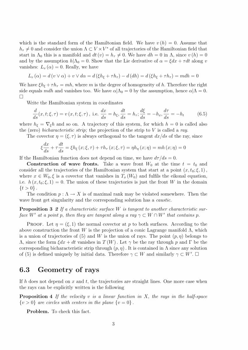
where hξ = ∇ξh and so on. A trajectory of this system, for which h = 0 is called alsothe (zero) bicharacteristic strip; the projection of the strip to V is called a ray.
The covector η = (ξ, τ) is always orthogonal to the tangent dx/ds of the ray, since
ξdx
ds+ τ
dt
ds= ξhξ (x; ξ, τ) + τhτ (x; ξ, τ) = ηhη (x; η) = mh (x; η) = 0
If the Hamiltonian function does not depend on time, we have dτ/ds = 0.Construction of wave fronts. Take a wave front W0 at the time t = t0 and
consider all the trajectories of the Hamiltonian system that start at a point (x, t0; ξ, 1) ,where x ∈ W0, ξ is a covector that vanishes in Tx (W0) and fulfils the eikonal equation,i.e. h (x, t0; ξ, 1) = 0. The union of these trajectories is just the front W in the domaint > 0 .
The condition p : Λ → X is of maximal rank may be violated somewhere. Then thewave front get singularity and the corresponding solution has a caustic.
Proposition 3 2 If a characteristic surface W is tangent to another characteristic sur-face W ′ at a point p, then they are tangent along a ray γ ⊂ W ∩W ′ that contains p.
Proof. Let η = (ξ, 1) the normal covector at p to both surfaces. According to theabove construction the front W is the projection of a conic Lagrange manifold Λ, whichis a union of trajectories of (5) and W is the union of rays. The point (p, η) belongs toΛ, since the form ξdx + dt vanishes in T (W ) . Let γ be the ray through p and Γ be thecorresponding bicharacteristic strip through (p, η) . It is contained in Λ since any solutionof (5) is defined uniquely by initial data. Therefore γ ⊂ W and similarly γ ⊂ W ′. ¤
6.3 Geometry of rays
If h does not depend on x and t, the trajectories are straight lines. One more case whenthe rays can be explicitly written is the following
Proposition 4 If the velocity v is a linear function in X, the rays in the half-spacev > 0 are circles with centers in the plane v = 0 .
Problem. To check this fact.
3
6.4 Legendre transformation and geometric duality
Definition. Let f : X → R be a continuous function; the function g defined in X∗ by
g (ξ).= sup
x
ξx− f (x)
is called Legendre transformation of f. If f is convex, g is defined in a convex subsetof the dual space and is also convex. If g is defined everywhere in X∗, the Legendretransformation of g coincides with f, provided f is convex. This means that the graphof f is the envelope of hyperplanes t = ξx− g (ξ) , ξ ∈ X∗.
If f ∈ C1 (X) an arbitrary function, the Legendre transformation is defined as follows
g (ξ) = ξx− f (x) as ξ = ∇f (x)
If f ∈ C2 (X) and det∇2f 6= 0 the equation ∇f (x) = ξ can be solved, at least, locallyand the Legendre transform is defined as a multivalued function.
Example. For a non-singular quadratic form q (x) = qijxixj/2 the Legendre trans-
form is again a quadratic form, namely, q (ξ) = qijξiξj/2, where qij is the inversematrix to qij . Indeed, the system ξi = ∂iq (x) = qijx
j is solved by xi = qijξj. Then theLegendre transform equals
ξiqijξj − qijq
ikqjlξkξl/2 = ξiqijξj/2 = q (ξ)
Definition. Let K be a compact set in X. The function
p∗K (ξ) = maxK
ξx
is called Minkowski functional of K. If K is convex and simmetric with respect to theorigin, the functional p∗K is a norm in X∗ and the Minkowski functional of the unit ballp∗K (ξ) ≤ 1 is equal to the norm pK in X generated by K.
Problem. Show that the Legendre transform of the function (pK)2 /2 is equal to
(p∗K)2 /2, provided K is convex.Definition. Let Y be a smooth conic hypersurface in X (i.e. Y is smooth in X\ 0).
The set Y ∗ of conormal vectors to Y \ 0 is a cone in X∗. It is called the dual conicsurface. If Y is strictly convex, i.e. the intersection H ∩Y is strictly convex for any affinehypersurface in X\ 0 , then Y ∗ is smooth strictly convex hypersurface too.
Exercise. To check that, if Γ is the interior of the convex hypersurface Y, then thedual cone Γ∗ as in Chapter 3 (MP3) is the interior of the Y ∗.
Problem. Let f be a smooth homogeneous function in V of degree d > 1 suchthat ∇f does not vanish in Y
.= f = 0 . Show that the Legendre transform g is a
homogeneous function of degree d/ (d− 1) that vanishes in the dual cone Y ∗.
6.5 Fermat principle
We have σ2 (x; ξ, τ) = q (x; ξ)− τ 2, where q is positive quadratic form of ξ. The Legendretransform of q/2 form with respect to ξ is the quadratic form q (x; y) /2, where
q (x; y) = gij (x) yiyj
4
Let γ be a smooth curve in the Euclidean space X given by the equation x = x (r) , a ≤r ≤ b; the integral
T (γ) =
∫ b
a
√
q (x (r) , x′ (r))dr
is called the optical length of the curve γ (or the action). It is equal to the time of amotion along γ with the velocity
√
q (x (r) , x′ (r)) (v = n−1 in the isotropical case).
Proposition 5 3 Each ray of the system (5) for the Hamiltonian function h = σ2/2 isan extremal of the optical length integral T (γ) .
Proof. We compare the Euler-Lagrange equation
d
dr
∂F
∂x′− ∂F
∂x= 0 (6.6)
for F =√
q (x, x′) with the system (5). Suppose for simplicity that the medium is
isotropic, i.e.√
q (x, x′) = n (x) |x′| , h (x; ξ, τ) =(
v2 (x) |ξ|2 − τ 2)
/2. Set
ξ =∂F
∂x′= n (x)
x′
|x′| ,d
ds=
1
n |x′|d
dr
The Euler-Lagrange equation turns to
dξ
ds=
1
n |x′|d
dr
∂F
∂x′=
1
n |x′|∂F
dx=∇nn |x′| = −∇v
2 |ξ|2 /2 = −h′x
since |ξ| = n, whereasdx
ds=
x′
n |x′| = v2ξ = h′ξ
These equations together with τ = 1, dt/ds = 1 give (5). ¤Exercise. To generalize the proof for the case of anisotropic medium.
Corollary 6 Snell’s law of refraction: n1 sinϕ1 = n2 sinϕ2.
Problem. To verify the Snell’s law by means of the Fermat principle.
Corollary 7 Rays of the equation (1) are geodesics of the metric g = gijdxidxj and vice
versa.
6.6 The major Huygens principle
The functionσ2 (x; η) = gij (x) ξiξj − τ 2, η = (ξ, τ)
is the principal symbol of the equation (1). Fix x and consider the coneK∗x
.= σ2 (x; η) = 0
in V ∗. It is called the cone of normals at x. The dual cone Kx in V ; it is called the coneof velocities at x. It is given by the equation h (x, y, y0) = 0, where
h (x; y, y0) =(
gij (x) yiyj − y02
)
/2
5
is the Legendre transform of h.= σ2/2 and (y, y0) stands for a tangent vector to V at
(x, t) .The major Huygens principle. Let W0 be a smooth wave front at a moment
t = t0. For a small time interval ∆t and an arbitrary point x ∈W0 take the ellipsoid
Sx.=
h (x; ∆x,∆t) = 0
(6.7)
Let W be the envelope of these ellipsoids. The claim: the wave front W∆t at the momentt = t0 +∆t coincides with a component of W up to O (∆t2) .
This means, in fact, that the distance between the hypersurfaces is O (∆t2) in thestandard C1-metric.
Proof. An arbitrary point x ∈ W0 is the end of a ray γ given by an equationx = x (t) , 0 ≤ t ≤ t0. According to (5), the extension of this ray for the time interval[t0, t0 +∆t] is approximated by the line interval [x, x] , where x = x + ∆t x′, x′ =hξ (x; ξ, 1) up to a term O (∆t2) and the point (x; ξ, 1) belongs to the bicharacrestic stripthat projects to γ. Check that the point x belongs to Sx; we have ∆t−2h (x,∆t x′,∆t) =h (x, x′, 1) , since h is a homogeneous quadratic function. By the involutivity of theLegendre transform, h is the Legendre transform of h, i.e.
h (x, x′, 1) = ξx′ + τ − h(
x; ξ, τ)
where the point(
ξ, τ)
satisfies hξ
(
x; ξ, τ)
= x′, hτ (x; ξ, τ) = 1. We find τ = 1 form the
second equation and ξ = ξ from the first equation. Therefore
h (x, x′, 1) = ξx′ + 1− h (x; ξ, 1) = ξhξ (x; ξ, 1) + hτ (x; ξ, 1)− h (x; ξ, 1) = h (x; ξ, 1) = 0
since h is homogeneous of degree 2. Therefore the point x ∈ Sx is close to the front W∆t.Take another point y = x+∆x ∈ Sx; consider the piecewise curve γy = γ ∪ ly where
ly denotes the interval [x, x+∆x] . The optical length of γy is equal the sum of opticallengths of the pieces, i.e. T (γy) = t0 +∆t = t. It is the same as for the front W∆t. Thepoint x+∆x belongs to a ray γ ′ that is close to γ. The time coordinate of this point in γ ′
is less that t+∆t since of the Fermat principle. Therefore this point is behind the frontW∆t. This completes the proof. ¤
6.7 Geometrical optics
This is the ray method (Debay’s method) and similar methods for construction of highfrequency approximations to solutions of the wave equation:
auω = O(
ω−q)
where a is a wave operator (1) or a similar operator. One looks for an approximatesolution of the form (WKB-form)
uω(x, t) = exp(ıω(ϕ(x) + t))(a0(x) + ω−1a1(x) + ...+ ω−kak(x)) = exp (ıωt)U (x, ω)
6
where the time frequency ω is a big parameter. Then the function
U(x, ω) = exp(ıω(ϕ(x)))(a0(x) + (ıω)−1 a1(x) + ...+ (ıω)−k ak(x)) (6.8)
is an approximate solution of the Helmholtz equation(
ω2 + gij∂i∂j + bj∂j + c)
U (x, ω) = O(
ω−k)
The phase function ϕ satisfies the eikonal equation 1− gij∂iϕ∂jϕ = 0 and the amplitudefunctions a0, a1, ..., ak fulfil the recurrent differential equations, called transport equations
2gij∂iϕ∂ja0 +(
∂igij∂j (ϕ) + bj∂jϕ
)
a0 = 0 :Ta0 = 0 (6.9)
2gij∂iϕ∂ja1 +(
∂igij∂jϕ+ bj∂jϕ
)
a1 = −(
∂igij∂j + bj∂j + c
)
a0
...
Tak = Lk (a0, ..., ak−1)
where the operator T = 2gij∂iϕ∂j + (∂igij∂j (ϕ) + bj∂jϕ) acts along geodesic curves of
the metric g. The principal term of (8) is called the approximation of geometrical optics.A caustic is an obstruction of the ray method.
6.8 Caustics
Take the manifold Λ in the phase space that is solution of the system (3)
h (x, t; η) |Λ = 0, α|Λ = 0
If dimΛ = n = dimV, it is called Lagrange manifold. Consider the projection p : Λ→ V ;the image W = p (Λ) is called wave front. A point (x, t) ∈ W is regular, if (x, t) =p (λ) , λ ∈ Λ and rank of p in λ is equal n − 1 for any λ. The set of singular points isclosed; its projection to X called the caustic of Λ.
6.9 Geometrical conservation law
We have found the conservation law for the global energy of a field u satisfying theselfadjoint wave equation (MP2) by means of
− ∂
∂t
⟨
∂2u
∂t2, u
⟩
= − ∂
∂t
∑
⟨
∂
∂xi
(
v2∂u
∂xi
)
, u
⟩
This identity can be written in the form
div Ix,t = 0, where Ix,t.=(
v2 (∇xuut − ut∇u) , utut
)
The space-time field Ix,t is interpreted as the energy current. For a time-harmonic solutionu (x, t) = exp (ıωt)U (x, ω) the last component drops out and ut = ıωu. Therefore theenergy current is represented by the field Ix = v2 (∇xuut − ut∇u) . For the arbitraryselfadjoint wave operator
(
∂2t − ∂igij∂j − c
)
u = 0
7
the energy current is
I i =ω
2√−1
gij(
∂jUU − U∂jU)
, i = 1, 2, 3
Substitute the WKB-development for (8) and take in account that the phase and ampli-tude functions are real:
I i = ω2gij∂jϕa0 +O (ω)
The vector gij∂jϕ = hξi(x,∇ϕ) = hξi
(x, ξ) = dxi/ds is equal to the tangent to the raythrough a point x ∈ X. It follows
Corollary 8 The energy flows along the rays in the approximation of geometrical optics.
This fact can be explained in a different way. Consider the transport equation for themain term of the amplitude
Ta0.= 2gij∂iϕ∂ja0 + ∂ig
ij∂j (ϕ) a0 = 0
and write it in the form2da0/ds+ ∂i
(
vi)
a0 = 0 (6.10)
where ∂ivi = div v (s) , and vi
.= hξi
= gij∂jϕ is the X-component of Hamiltonian fieldthat generates the geodesic flow (5). We have div v (s) = (V (s))−1 dV (s) /dswhere V (s)is the image of the volume element dx in X. Indeed, we have
Lv (dx) = d (v ∨ dx) = div (v) dx
Therefore (10) is equavalent tod
ds
(
a0√dx)
= 0
i.e. the halfdensity a0√dx is preserved by the geodesic flow. The square of this haldehsity
is the energy density∣
∣
∣a0√dx∣
∣
∣
2
= |a0|2 dx of the wave field.
Corollary 9 The energy density is preserved by the geodesic flow.
Another conclusion is: a solution of the Helmholtz equation can be considered a half-density, whose square is the energy density. Also the halfdensity a0
√dx ∧ dt is preserved
by this flow since dt is constant, since vt = ht = 0. Therefore a solution of the waveequation is a halfdensity in space-time.
8
Chapter 7
The method of Fourier integrals
7.1 Elements of simplectic geometry
Cotangent bundle. Let M be a manifold. Consider the set T ∗(M) = ∪MT∗x (M)
together with the mapping p : T ∗(M) → M that maps the fibre T ∗x (M) to the pointx. It maps an arbitrary element ω ∈ T ∗x (M) to the point x. The pair T ∗(M), p) iscalled cotangent bundle of the manifold M . The bundle possesses a smooth atlas: for anarbitrary chart (U, ϕ) in M one takes the set T ∗(U) as the domain of a chart in T ∗(M).Each element ω ∈ T ∗x (M) can be written in the form ω =
∑m
1 ξjdxj, where the coefficientsξi ∈ are uniquely defined. The mapping
ϕ p× ξ : p−1(U) → Rm × Rm, ξ(ω) = (ξ1, ..., ξm) (7.1)
is a chart in T ∗(M). For another chart (U ′, ϕ′) of this kind holds the relation ψϕ′ = ϕ,where the transition mapping ψ is of the form ψ((ξ1, ..., ξn), x) = (ξ′1, ..., ξ
′n), x). Here ξ′i
are coefficients of cotangent vectors in the second chart: ω =∑
ξ′idx′i. They are related
to the coefficients in the first charts:
ξj(ω) =∑ ∂x′i
∂xjξ′i(ω)
Here J = ∂x′i/∂xj is again the Jacobi matrix of the transition mapping ψ. Consequentlythe relation between the coefficients is linear and smooth with respect to the coordinatesin U (as well as in U ′). Therefore the transition mapping belongs to the class C∞ andT ∗(M) has a smooth structure. The natural projection p : T ∗(M) → M is a mappingof smooth manifolds. Each fibre p−1(x) = T ∗x (M) is a vector space (hence T ∗(M) is avector bundle).Remark. The union of sets Tx(M), x ∈ M has a structure of vector bundle too. It iscalled tangent bundle.Canonical forms. The 1-form αU =
∑
ξidxi is defined for each chart (1). For anotherchart in p−1(U ′) the forms αU and αU ′ coincide in the intersection p−1(U)∩p−1(U ′). Thisfollows from (2). Therefore there is well-defined a 1-form α in T ∗(M) such that α = αU
for each chart U . It is called canonical 1-form in T ∗(M).The form σ = dα is called canonical 2-form in the simplectic manifold T ∗(M). It isclosed: dσ = 0. In local coordinates σ =
∑m
1 dξi ∧ dxi.
1
Definition. Let M be a manifold of dimension m. A submanifold Λ ⊂ T ∗(M) is calledLagrange manifold, if it satisfies the conditions dim Λ = m and σ|N = 0.
Proposition 1 1 Let Λ be a Lagrange manifold in T ∗(M) and λ ∈ Λ be a point thatis not a critical point of the projection p : Λ → M . There exists a neighborhood U ofy = π(λ) and a real smooth function f in U such that the set of solutions of the system
ξi =∂f
∂xi, i = 1, ...,m (7.2)
coincides with Λ in a neighborhood of λ.
Proof. Let U be a simply connected neighborhood U of y such that the projectionp is a diffeomorphism pU : Λ(U) → U , where we denote Λ(U) = Λ ∩ π−1(U). Take apoint ξ ∈ Λ(U) and join the point x = p(ξ) with the point y by a curve γx ⊂ U . We liftthis curve by means of the mapping (pU)−1 and get a curve Γ ⊂ Λ(U), which join thepoint ξ with λ. The integral f(λ) =
∫
Γα does not depend on the choice of the curve γx,
because of the set Λ(U) ∼ U is simply connected and the form σ = dα vanishes in Λ.The function f is a primitive of the form α in U , i.e. df = (pU)−1∗α. This is equivalentto (2). ¤Definition. We call the image of projection p : Λ → M of a Lagrange manifold Λ thelocus (or front) of this manifold. In the case of previous Proposition the locus is an openset in M . In the general case it is subset with singularities.Definition. Denote by T ∗0 (M) the open subset in T ∗(M) of pairs (x, ξ), ξ 6= 0 .Themultiplicative group of positive numbers + = t > 0 acts in T ∗0 (M) as follows t :(x, ξ) 7→(x, tξ). A trajectory of the group + is called ray. A subset K ⊂ T ∗0 (M) is calledconic, if K is invariant with respect to the group, i.e. is a union of rays. We note that noconic Lagrange manifold can satisfy the conditions of Proposition 1. We generalize thisproposition in the next section.
Proposition 2 2 A conic submanifold Λ of dimension dimM is a Lagrange manifold ifand only if the canonic 1-form α vanishes in Λ.
Proof. The part ”if” is obvious: σ|K = dα|K = d(α|K) = 0. We need to check thatthe equation σ|Λ = 0 implies α|Λ = 0. Consider the field e =
∑
ξi∂/∂ξi (Euler field)in the cotangent bundle. It satisfies the equation e ∨ σ = α. The Euler field is tangentto rays and hence to any conic submanifold. Therefore for any field v in T ∗(M) that istangent to Λ we have
α(v) = v ∨ α = v ∨ (e ∨ σ) = σ(e, v) = 0
Example. Let P be a submanifold of manifold M . Consider the set N ∗P (M) ⊂ T ∗(M) of
points (x, ξ), x ∈ P such that the form∑
ξidxi vanishes in Tx(P ). It is called conormalbundle to P . This is obviously a conic Lagrange manifold.
2
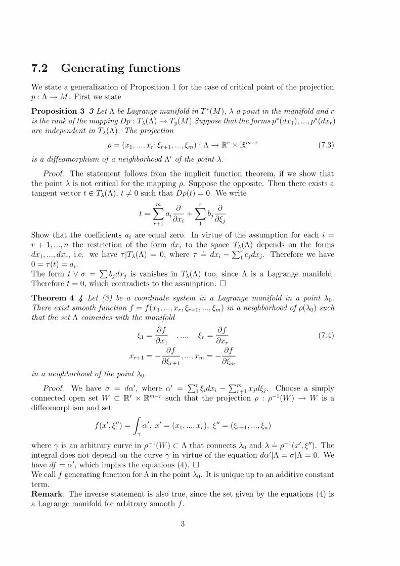
7.2 Generating functions
We state a generalization of Proposition 1 for the case of critical point of the projectionp : Λ →M . First we state
Proposition 3 3 Let Λ be Lagrange manifold in T ∗(M), λ a point in the manifold and ris the rank of the mapping Dp : Tλ(Λ) → Ty(M) Suppose that the forms p∗(dx1), ..., p
∗(dxr)are independent in Tλ(Λ). The projection
ρ = (x1, ..., xr; ξr+1, ..., ξm) : Λ → Rr × Rm−r (7.3)
is a diffeomorphism of a neighborhood Λ′ of the point λ.
Proof. The statement follows from the implicit function theorem, if we show thatthe point λ is not critical for the mapping ρ. Suppose the opposite. Then there exists atangent vector t ∈ Tλ(Λ), t 6= 0 such that Dρ(t) = 0. We write
t =m∑
r+1
ai∂
∂xi+
r∑
1
bj∂
∂ξj
Show that the coefficients ai are equal zero. In virtue of the assumption for each i =r + 1, ..., n the restriction of the form dxi to the space Tλ(Λ) depends on the formsdx1, ..., dxr, i.e. we have τ |Tλ(Λ) = 0, where τ
.= dxi −
∑r
1 cjdxj. Therefore we have0 = τ(t) = ai.The form t ∨ σ =
∑
bjdxj is vanishes in Tλ(Λ) too, since Λ is a Lagrange manifold.Therefore t = 0, which contradicts to the assumption. ¤
Theorem 4 4 Let (3) be a coordinate system in a Lagrange manifold in a point λ0.There exist smooth function f = f(x1, ..., xr, ξr+1, ..., ξm) in a neighborhood of ρ(λ0) suchthat the set Λ coincides with the manifold
ξ1 =∂f
∂x1, ..., ξr =
∂f
∂xr(7.4)
xr+1 = −∂f
∂ξr+1, ..., xm = −
∂f
∂ξm
in a neighborhood of the point λ0.
Proof. We have σ = dα′, where α′ =∑r
1 ξidxi −∑m
r+1 xjdξj. Choose a simplyconnected open set W ⊂ Rr × Rm−r such that the projection ρ : ρ−1(W ) → W is adiffeomorphism and set
f(x′, ξ′′) =
∫
γ
α′, x′ = (x1, ..., xr), ξ′′ = (ξr+1, ..., ξn)
where γ is an arbitrary curve in ρ−1(W ) ⊂ Λ that connects λ0 and λ.= ρ−1(x′, ξ′′). The
integral does not depend on the curve γ in virtue of the equation dα′|Λ = σ|Λ = 0. Wehave df = α′, which implies the equations (4). ¤We call f generating function for Λ in the point λ0. It is unique up to an additive constantterm.Remark. The inverse statement is also true, since the set given by the equations (4) isa Lagrange manifold for arbitrary smooth f .
3
Proposition 5 5 The Lagrange manifold generated by a function f is conic if f ishomogeneous function of coordinates ξr+1, ..., ξm of degree 1. Inversely any conic Lagrangemanifold is generated by a homogeneous function of degree 1 in a conic neighborhood ofa given point λ0.
Proof. Let f be homogeneous function of degree 1. Each derivative ∂f/∂xj is homo-geneous of degree 1 too and any derivative ∂f/∂ξi is homogeneous of degree 0. Thereforefor arbitrary solution (x, ξ) any point (x, tξ), t > 0 satisfies the system (4).Inversely, if Λ is conic, we can take a conic neighborhood W of the projection of the pointλ0 = (x0, ξ0). Define a generating function f by means of the integral as above takenover a curve γ from the point (x0, 0) to λ. This is a generating function too. Check thatit is homogeneous. Really for any λ = (x, ξ) we can take the curve γ = g ∪ r, where gjoins the points x0 and x and r is the ray (x, tξ), 0 ≤ t ≤ 1. Therefore
f(ρ(λ)) =
∫
γ
α′ =
∫
r
α′ =m∑
r+1
xjξj,
where xr+1, ..., xm are functions of x1, ..., xr.
7.3 Fourier integrals
Fourier integral in an open set X ⊂ Rn is a functional of the form
I(φ, a)ψ =
∫
X
∫
Θ
exp(2πıφ(x, θ))a(x, θ)dθψ(x)dx, ψ ∈ D(X) (7.5)
The function φ is called phase and a amplitude. They are defined in X ×Θ, where X isan open set in Rn and Θ = RN \ 0 is named ancillary space. The group R+ of positivenumbers acts in the space X × Θ by (x, θ) 7→(x, tθ). Any set (x, tθ), t > 0 is calledray ; a conic set is a union of rays. A function f defined in X×Θ is termed homogeneousof degree d, if f(x, tθ) = tdf(x, θ) for t > 0. The phase function is supposed to be realand homogeneous of degree 1.We suppose that the amplitude satisfies the estimate a(x, θ) = O(|θ|µ) for some µ thatis locally uniform with respect to x ∈ X. If µ + N < 0, the integral over the ancillaryspace converges and
|I(φ, a)(ψ)| ≤
∫
C(x)|ψ(x)|dx (7.6)
for some positive continuous function C. If the integral Fourier does not convergesabsolutely we apply a regularization procedure to turn it to a continuous functional inthe space D(X). For this we suppose that the amplitude satisfies some special conditions.Definition. Let µ, ρ ∈ R, 0 < ρ ≤ 1. The class Sµ
ρ = Sµρ (X × Θ) is the set of functions
a in X ×Θ that satisfy for arbitrary i ∈ Zn+, j ∈ ZN
+
∣
∣DixD
jθa(x, θ)
∣
∣ ≤ Cij(x)(|θ|+ 1)µ−ρ|j|, (7.7)
with a continuous function Cij that does not depend on θ. We call the number ν.= µ+N/2
order of the Fourier integral I(φ, a).
4
Example. An arbitrary smooth homogeneous amplitude a of degree µ belongs to Sµ1 .
Definition. We say that an amplitude a is asymptotical homogeneous of order µ, if ithas for any q the following development:
a = aµ + aµ−1 + ...+ aµ−q + rq,
where each term aν is a smooth homogeneous amplitude of degree ν and rq ∈ Sµ−q−11 .
We regularize the Fourier integral in following way:
I(φ, a)(ψ) = limε0
∫
X
∫
Θ
exp(2πıφ(x, θ)− ε|θ|)a(x, θ)ψ(x)dθdx (7.8)
The integral in righthand side obviously converges to any ε > 0.Let q ≥ 0 be an integer; we say that a distribution u ∈ D′(X) is of singular order ≤ q, if
|u(ψdx)| ≤∑
|i|≤q
∫
X
C(x)∣
∣Diψ(x)∣
∣ dx
for a continuous function C. In particular, (6) implies that the distribution I(φ, a) is ofsingular order ≤ 0.
Theorem 6 Let φ be arbitrary smooth real homogeneous of degree 1 function in X ×Θwithout critical points and a ∈ Sµ
ρ . The limit (8) exists for any test function ψ. Thefunctional I(φ, a) is a distribution of singular order ≤ q, if µ+N < qρ.
Remark. At this stage we can consider the Fourier integral as a functional in thespace D(X) of test densities ρ = ψdx as well. From this point of view the Fourierintegral is a generalized function. A more natural approach is to handle it as a generalizedhalfdensity.
Proof. We call a differential operator A in X × Θ homogeneous of degree α, if thefunction Af is homogeneous of degree d+ α for an arbitrary homogeneous function f ofarbitrary degree d. In particular, the fields
b(x, θ)∂
∂xi, i = 1, ..., n, c(x, θ)
∂
∂θj, j = 1, ..., N
are homogeneous operators of degree −1, if the functions b(x, θ) and c(x, θ) are homo-geneous of degree −1 and 0 respectively. The condition (7) implies that for arbitraryhomogeneous operator A of degree −1 and amplitude a ∈ Sµ
ρ we have Aa ∈ Sµ−ρρ .
Pick out a function χ ∈ D(RN) such that χ(θ) = 1 for |θ| ≤ 1. Write (5) in the formof sum of two integrals with the extra factors χ and 1 − χ. The first one is a properintegral which converges to [I0dx](ψ) as ε→ 0, where
I0(x) =
∫
exp(2πıφ(x, θ))χ(θ)a(x, θ)dθ
is a continuous function. Set φε = 2πφ+ ıε|θ|.
5
Lemma 7 There exists a smooth family of tangent fields vε, ε ≥ 0 of degree −1 in X×Θsuch that vε(φε) = −ı.
We postpone a proof of this Lemma. Write the second integral as follows∫ ∫
exp(ıφε)(1− χ)aψdxdθ =
∫ ∫
vε(exp(ıφε))(1− χ)aψdxdθ
Integrating by parts the right side, we get the integral∫ ∫
exp(ıφ)v∗((1− χ)aψ)dxdθ,
where v∗ denotes the conjugated differential operator. This is an operator of degree −1and we have
v∗ε((1− χ)aψ) = [vε(χ)− div(vε)(1− χ)]aψ − (1− χ)(vε(a)ψ + avε(ψ)),
whence
∫ ∫
exp(ıφε)(1− χ)aψdxdθ =
∫ ∫
exp(ıφε)
[
a0ψ +∑
j
aj∂ψ
∂xj
]
dxdθ, (7.9)
anda0 = [vε(χ)− div(vε)(1− χ)]a+ vε(a), aj = −avε(xj), j = 1, ..., n
The amplitude aj, j = 1, ..., n belong to the class Sµ−1ρ and satisfy (7) with constants
Cij that do not depend on ε, since the function vε(xj) is smooth and homogeneous ofdegree −1. The same is true for the function [vε(χ) − div(vε)(1 − χ)]a since div(vε) ishomogeneous of degree −1 and vε(χ) has compact support. The function vε(a) belongs tothe space Sµ−ρ
ρ and satisfy the corresponding inequality (7) with some constants that donot depend on ε. Taking in account the inequality ρ ≤ 1, we conclude that the functionsa0, ..., an satisfy (7) with some uniform constants and with the exponent µ− ρ instead ofµ. If µ+N < ρ, the integrals
∫
exp(ıφε)|aj|dθ, j = 0, 1, ..., n
converges uniformly with respect to ε and we can pass on to the limit in (9). Thus weget the inequality
| limε0
∫
Θ
∫
X
exp(ıφε)a(x, θ)ψ(x)dxdθ ≤ C
[
∫
|ψ|dx+n∑
1
∫∣
∣
∣
∣
∂ψ
∂xj
∣
∣
∣
∣
dx
]
where the constant C does not depend on ε. It follows that I(φ, a) is a distribution oforder ≤ 1.If the opposite inequality µ + N ≥ ρ holds, we apply the same method to each term of(9) and get
I(φε, a)(ψ) =
∫
exp(ıφε)∑
ij
[
a00ψ +∑
a0j∂ψ
∂xj+∑
aij∂2ψ
∂xi∂xj
]
dxdθ,
6
where the amplitudes aij belong to Sµ−2ρρ and satisfy (7) uniformly with respect to ε. We
repeat these arguments q times until we reach the inequality µ+N < qρ. ¡
Proof of Lemma 1. We set
v =∑
bj∂
∂xj+∑
ci∂
∂θi,
where
bj = −ı
σ
∂φ
∂xj, ci = −
ı|θ|2
σ
∂φ
∂θi, σ =
∑
∣
∣
∣
∣
∂φ
∂xj
∣
∣
∣
∣
2
+ |θ|2∑
∣
∣
∣
∣
∂φ
∂θi
∣
∣
∣
∣
2
The dominator σ does not vanish. We have v(φε) = −ı−εv(|θ|) where the function v(|θ|)is homogeneous of degree 0. We set vε = (1 + εıv(|θ|))−1v. ¡
Lemma 8 Let u be an arbitrary homogeneous tangent field in X×Θ of degree −1 and Ωa smooth differential form of the highest degree in X×Θ that vanishes in the complementof K × Θ for a compact set K ⊂ X such that the forms Ω and LuΩ are integrable. Wehave
∫
Lu(Ω) = 0 (7.10)
Proof. Suppose that the form Ω has compact support and state the equation
∫
Φ∗t (ω) =
∫
ω (7.11)
for small t, where Φt means the flow generated by the field u. The integral of a form ofthe highest degree is invariant with respect to any isomorphism of the manifold. Take thet-derivative of (11) and get (10). For the given form Ω we consider the product Ωk = hkΩwhere hk(θ) = h(k−1θ). The integral
∫
Ωk converges to∫
Ω as k →∞. We have
0 =
∫
Lu(Ωk) =
∫
u(hk)Ω +
∫
hkLu(Ω)
We have∫
hkLu(Ω) →∫
Lu(Ω) as k → ∞. At the other hand u(hk) =∑
cj∂hk/dθj =O(k−1) uniformly in X ×Θ, since the functions cj = u(θj), i = 1, ..., N are homogeneousof degree 0. Therefore
∫
u(hk)Ω → 0. ¤Example. Let X be an open set in Rn, x1, ..., xn are coordinate functions. Take Ω =fgdx ∧ dθ in (10) and get
∫
u(f)gdxdθ =
∫
fu∗(g)dxdθ, (7.12)
where the sum
u∗ = −u− div u, div u ≡Lu(dx ∧ dθ)
dx ∧ dθ=∑ ∂bj
∂xj+∑ ∂ci
∂θi
7
is the conjugated differential operator to the field u. We check the last equation by meansof (4.4.8):
Lu(fgdx ∧ dθ) = u(f)gdx ∧ dθ + fu(g)dx ∧ dθ + fgLu(dx ∧ dθ)
Lu(dx ∧ dθ) = d(u ∨ (dx ∧ dθ)) =∑
j
(−1)j−1d(bjdx1 ∧ ...... ∧ dxn ∧ dθ)
+∑
i
(−1)n+i−1d(cidx ∧ dθ1 ∧ ...ı... ∧ dθN) = div(u) dx ∧ dθ
Remark. We can use instead of Eε = exp(−ε|θ|) another sequence of decreasing func-tions, f.e. Eε = exp(−ε|θ|2) in (8) . We get the same limit.Non-degenerate phase. Let φ be a phase function in X ×Θ. Consider the set
C(φ) = (x, θ) : dθφ = 0, ⇐⇒ φ′θ1 = ... = φ′θN= 0
where φ′θj
.= ∂φ/∂θj. This is the critical set of the projection φ = 0 → X.
Definition. The phase function φ is called non-degenerate, if it has no critical pointsand the differential forms
d(
φ′θ1)
, ..., d(
φ′θN
)
are linearly independent in each point of the set C(φ). Suppose that φ is a non-degeneratephase. The critical set C(φ) is a conic subset of X × Θ of dimension n + N −N = n =dimX. This follows from the Implicit function theorem. Recall that T ∗ (X) means thesubset of T ∗(X) of nonzero cotangent vectors. Consider the mapping
φ∗ : C(φ) → T ∗ (X), (x, θ) 7→(x, dxφ(x, θ))
It is well-defined since dxφ does not vanish in the set, where dθφ = 0. This mapping ishomogeneous of degree 1, since dxφ(x, tθ) = tdxφ(x, θ) for t > 0.
Proposition 9 The differential Dφ∗ : T (C(φ)) → T (T ∗ (X)) of the mapping φ∗ is injec-tive in each point of C(φ).
Proof. The injectivity of Dφ in a point (x, θ) ∈ C(φ) is equivalent to the followingimplication:
v ∈ T(x,θ)(C(φ)), Dφ∗(v) = 0 =⇒ v = 0
Write v = t+ τ, t ∈ Tx(X), τ ∈ Tθ(Θ) and calculate by means of local coordinates in X:
0 = Dφ∗(v) =(
t; v(φ′x1), ..., v(φ′xn
))
∈ Tω(T ∗ (X)) (7.13)
We denote here ω = (x, dxφ(x, θ)) and use the natural isomorphism
Tω(T ∗(X)) ∼= Tx(X)⊕ Rn
From (12) we conclude that t = 0 and τ(φ′xj) = 0, j = 1, ..., n At the other hand the
vector τ = v is tangent to C(φ), which means
τ(φ′θi) = 0, i = 1, ..., N
8
Extend the vector τ to the constant vector field τ in Θ. It commutes with the coordinatederivatives in X × Θ, consequently the last equations are equivalent to the followingdθτφ(ω) = 0. This is a linear relation between the forms dφ′θ1 , ..., dφ
′θN
. This relation isin fact trivial, since the phase φ is non-degenerate. ¤
Denote by Λ(φ) the image of the mapping Dφ∗. Take an arbitrary point (x0, θ0) ∈X ×Θ. In virtue of Implicit function theorem there exists a neighborhood X0 of x0 anda neighborhood Θ0 of θ0 such that the restriction of Dφ∗ to X0×Θ0 is a diffeomorphismto its image Λ0. We can take for Θ0 a conic neighborhood since the mapping Dφ∗ ishomogeneous. The image Λ0 is a conic submanifold of dimension n = dimX; it is closedin a conic neighborhood of the point ω0 = φ∗(x0, θ0). The variety Λ(φ) is a union ofpieces Λ0, hence it is a conic set too. If a neighborhood X1 ×Θ1 overlaps with X0 ×Θ0,then its image Λ1 is a continuation of the manifold Λ0. Taking a chain of continuationsΛ0,Λ1, ... we can reach a self-intersection point, if the mapping Dφ∗ is not an injection.In this case the set ÃL(φ) may have singular points and we call it variety.
Proposition 10 The set Λ(φ) is closed and locally equal a finite union of conic Lagrangemanifolds.
Proof. Show that the canonical 1-form α vanishes in any vector w ∈ T(x,ξ)(T∗(X)),
which belongs to the image of a tangent space T(x,θ)(C(φ)). We have ξ = dxφ(x, θ) andw = Dφ∗(v) for a tangent vector v to C(φ) at the point (x, θ). Therefore v(f) = 0 forarbitrary function f that vanishes in C(φ). Let t be the projection of w to X; it is equalthe projection of v. We calculate
α(w) = ξdx(t) = dxφ(t) = t(φ) = v(φ),
where the righthand side is taken at the point (x, θ) ∈ C(φ). It is equal zero, because ofthe function φ vanishes in C(φ). The last fact follows form the Euler identity φ =
∑
θiφ′θi
.It follows that any piece Λ0 of the set Λ(φ) is a Lagrange manifold.Take an arbitrary point ω ∈ Λ(φ), a neighborhood U of the point x = p(ω) such that itsclosure K is compact and check the set ΛK
.= Λ(φ)∩p−1(K) is closed. For this we take the
unit sphere S(Θ) in the ancillary space and consider the mapping φ∗ : C(φ)∩ (K×S(Θ))→ LK). It is continuous and the first topological space is compact. Therefore the imageis a closed subset of Λ(φ). The conic set Lk(φ) is generated by this subset and hence isalso closed.Show that ΛK is covered by a finite number of Lagrange manifolds. The set K ×Θ canbe covered by a finite number of conic neighborhoods Xq × Θq, q = 1, ..., Q as above.The restriction of the mapping φ∗ to each neighborhood of this form is a diffeomorphismto its image in virtue of the Implicit function theorem. The set ΛK is contained in theunion of Lagrange manifolds φ∗(Xq ×Θq), which implies our assertion. ¤
Proposition 11 Let Λ be a conic Lagrange manifold. For any point λ ∈ Λ there existsa non-degenerate phase function φ such that λ ∈ Λ(φ) ⊂ Λ.
Proof. Take the generating function f =∑m
k+1 fjξj at λ constructed in Proposition4.8.2 and consider θ = (ξk+1, ..., ξm) as ancillary variables. Here fj = fj(x
′, θ), j =k + 1, ..., n are smooth functions in W such that the equations
xj = fj(x′, θ), j = k + 1, ...,m (7.14)
9
are satisfied in Λ. We set
φ(x, θ).=∑
xjξj − f(x′, θ) =m∑
k+1
(xj − fj)ξj
and have ∂φ/∂ξj = xj − ∂f/∂ξj = xj − fj(x′, θ), hence the critical set C(φ) coincides
with (13) and φ is non-degenerate. Calculate the x-derivatives:
dxφ(x, θ) = (−dx′f, θ) = (ξ′(x′, θ), θ) = ξ|Λ
7.4 Lagrange distributions
Definition. Let X be an open set in Rn and Λ be a closed conic Lagrange submanifoldin T ∗ (X). We call an element u ∈ D′(X) Λ-distribution, (or Lagrange distribution), if itcan written as a locally finite sum of Fourier integrals:
u =∑
I(φj, aj) + v, v ∈ C∞,
where for each j the phase φj is non-degenerate in X ×Θj and
Λ(φj) ⊂ Λ, aj ∈ Sµj
ρ (X ×Θj)
Definition. Suppose that all amplitudes are asymptotical homogeneous. We shall saythat the Lagrange distribution u is of order ≤ ν, if u admits such a representation whereall the Fourier integrals I(φj, aj) are of the order ≤ ν.
Example 5.2. Let Y be a closed submanifold of X given by the equations f1(x) =... = fm(x) = 0 such that the forms df1, ..., dfm are independent in each point of Y .Consider the functional
δY (ρ) =
∫
Y
ρ
df1 ∧ ... ∧ dfm
on the space D(X) of test densities. The quotient is a density σ in Y such that df1∧ ...∧dfm ∧ σ = ρ, hence the integral is well-defined. It is called the delta-function in Y .Show that the delta-function is a Fourier integral with N = m if X is an open set inRn. Take the phase function φ(x, θ) =
∑m
1 θjfj(x) and the amplitude a = 1. In the casen = 1 we have for any test density ρ = ψdx
I(ρ) =
∫ ∫
exp(2πıθf(x))dθψ(x)dx =
∫
exp(2πıθy)dθψ
f ′dy,
if we take y = f(x) as an independent variable. The θ-integral is equal the delta-function,hence Iρ = ρ/df |f = 0, where ρ/df is a smooth function. In the case m > 1 we usethis formula m times and get
Iρ =
∫ ∫
exp(2πıφ(x, θ))dθρ =
∫
Y
ρ
df1 ∧ ... ∧ dfm= δY (ρ)
where δY is the delta-function in the manifold Y . This is a Λ-distribution of order(dimX − dimY )/2 for Λ = N ∗
Y .
10
Properties. For a conic Lagrange manifold Λ we denoteD′(Λ) the space of Λ-distributions.I. We have WF (u) ⊂ Λ for any u ∈ D′(Λ) according to Theorem 5.2.1.Problem. Let Λ be an arbitrary closed conic Lagrange manifold and λ ∈ Λ be an arbi-trary point. To show that there is an element u ∈ D′Λ such that λ ∈WF (u).II. For any u ∈ D′(Λ) and any smooth differential operator a in X we have au ∈ D′(Λ).If u is of order ≤ ν, then Pu is of order ν +m, where m is the order of a.III. Restriction to a submanifold. Let Y be a closed submanifold in X such thatΛ ∩N ∗(Y ) = ∅. Denote
ΛY = (y, η) : y ∈ Y, η = ξ|Ty(Y ), (y, ξ) ∈ Λ
This is a conic Lagrange submanifold in T ∗(Y ).
Proposition 12 Any Λ-distribution u has a restriction uY that is a ΛY -distribution. Ifu is of order ≤ ν, the distribution uY is of order ≤ ν too.
IV. Product. If Λ′ is another conic Lagrange manifold with no common points with−Λ, then for any Λ-distribution u and any Λ′-distribution u′ the product uu′ is well-defined as a distribution in X.
7.5 Hyperbolic Cauchy problem revisited
Consider a hyperbolic differential equation of order m in a space-time X = X0×R, whereX0 is an open set in Rn
a(x, t;Dx, Dt)u = w (7.15)
with smooth coefficients in X; x = (x1, ..., xn) are spacial coordinates, t is the timevariable. We denote by ξ, τ the corresponding coordinates for cotangent spacial and timevectors respectively. The principal symbol σm = σm(x, t; ξ, τ) of (14) is a polynomial invariables ξ, τ . We suppose that it has order m with respect to τ , which means that anyhypersurface t = const is non-characteristic for P . Consider the Cauchy problem in thedomain t > 0 with the initial data
u(x, 0) = v0(x),∂u(x, 0)
∂t= v1(x), ...,
∂m−1u(x, 0)
∂tm−1= vm−1(x), (7.16)
where v0, ..., vm−1 are some distributions.
Theorem 13 (Uniqueness) Any strictly hyperbolic Cauchy problem (14),(15) has nomore than one solution.
Fix a point y ∈ X0; let Ejy ∈ D
′(X×R+), j = 0, ...,m−1 be the solution of the initialproblem with w = 0, vi = δijδy. The set of distributions E0
y , E1y , ..., E
m−1y in X ×+ ×X
is called fundamental solution of the Cauchy problem. Then one can solve the Cauchyproblem with w = 0 and arbitrary distributions u0, ..., um−1 by means of integration:
u =∑
k
∫
X0
Ekyvk(y)dy
11
This formula is valid, at least, for distributions vk with compact support. In the globalcase we need an assumption on domain of dependence (see below). The general case isreduced to the case w = 0 by means of the Duhamel’s method.Remark. If the coefficients of the operator a do not depend on time, it is sufficient toconstruct the distribution Em−1
y only, since we have Eky = qm−1−k(y,D)Em−1
y , k < m− 1,where qj is an appropriate differential operator of order j. Then the distribution Ey =Em−1y is called the fundamental solution.
We describe now a more general construction. Therefore we can represent the symbolas the product of binomials:
σm(x, t; ξ, τ) = q0(x, t)m∏
1
[τ − τj(x, t; ξ)],
where τ1, ..., τm are homogeneous functions of variables ξ of degree 1 and q0 6= 0. LetΛ0 ⊂ T ∗ (X0) be an arbitrary Lagrange manifold. For any number j = 1, ...,m we considerthe Hamiltonian function hj(x, t; τ, ξ) = τ − τj(x, t; ξ) in T ∗(X × R+). We ”lift” Λ0 tothe bundle T ∗(X × R) taking the manifold
Wj = (x, 0; ξ, τj(x, 0; ξ)), (x, ξ) ∈ Λ
which is contained in the hypersurface hj = 0. The canonical form α vanishes in Wj.Now we take the Hamiltonian flow generated by hj
dx
dt=∂hj∂ξ
,dξ
dt= −
∂hj∂x
dτ
dt= −
∂hj∂t
(7.17)
with initial data from Wj. Denote by Λj the union of trajectories of this flow. This is aLagrange manifold Λj in T ∗(X×)R in virtue of Proposition ?4.7.1. The union Λ = ∪m
1 Λj
is also a Lagrange manifold possibly with self-intersection. Note that hj vanishes in Wj
and hence in Λj, since it is constant on any trajectory of (16).
Theorem 14 There exists a neighborhood Y of the hyperplane X0 in X such that forarbitrary Λ0-distributions v0, ..., vm−1 the Cauchy problem (14),(15) has a solution u thatis a Λ-distribution in Y . If vk is a Λ0-distribution of order ≤ ν + k for some ν andk = 0, 1...,m− 1, then the solution u is of order ≤ ν.
Proof. We describe in short the construction of u. Take an arbitrary point λ ∈ Λ0,a local coordinate system (x′, θ) for Λ0, where x′ = (x1, ..., xr) and θ = (ξr+1, ..., ξn),N = n−r. Let (x′0, θ0) be the coordinates of λ and x0
.= p(λ) ∈ X0. Take a phase function
φ0 = φ0(x, θ) in a conic neighborhood of (x0, θ0) that generates Λ0 in a neighborhood of λ.We can write the initial data v0, ..., vm−1 as Fourier integrals with the phase function φ0and some asymptotical homogeneous amplitudes b0, ..., bm−1 in a neighborhood of (x0, θ0),where bk is of order ≤ ν − N/2 + k for k = 0, ...,m − 1. The functions (x′, t; θ) form alocal coordinate system in Λj for any j and we can choose a generating phase function inthe form φj such that φj(x, 0; θ) = φ0(x, θ). Set uj,λ
.= I(φj, aj), where aj are unknown
homogeneous amplitudes of degree ν −N/2 and substitute it in the equation. We get aΛ-distribution w = auj,λ with the symbol
σ(w) =∑
j
(−ıL+ s)σ(uj,λ),
12
where L = Lpmis the Lie derivative. The term of degree ν + m vanishes according to
Proposition 5.6.1 since the symbol σm =∏
hk vanishes in Λj. The next term is calculatedby means of Theorem 6.1.1. where s is the subprincipal symbol of P . The degree of thisterm is equal ν + m − 1. We choose the amplitudes aj in such a way that the symbolof w vanishes. For this we solve first the equations (−ıL+ s)σ(uj) = 0. According to(5.5.1) we have σ(u) = ajψj, where ψj is a non-vanishing halfdensity depending only onthe phase function φj and aj be the principal homogeneous term of Aj of degree ν−N/2.Dividing the above equation by this halfdensity we get an equation
L(aj) + gjaj = 0 (7.18)
where gj is a known function. This is an ordinary equation along the trajectories of thefield (16). It has a unique solution for an arbitrary initial data aj(x, 0; θ). We specifythese data to satisfy the initial condition (15) for the Cauchy problem. This gives theequations
(2πı)k∑
j
(φ′j)kaj,λ(x, 0; θ) = gλ(x, θ)bk(x, θ), k = 0, ...,m− 1, (7.19)
where we denote φ′ = ∂φ/∂t and introduce a factor gλ that is a smooth homogeneousfunction of degree 0 supported by a compact conic neighborhood V of (x0, θ0) (i.e. theintersection supp gλ ∩ S
∗(X0) is compact). In the k-the equation both sides are homo-geneous of the same degree ν − N/2 + k. To solve this system we consider the matrixW = (φ′j)
k, where φ′ = dφ/dt. We have
detW =∏
j<k
(φ′j − φ′k),
hence the matrix W is invertible, if φ′j 6= φ′k for j < k. We have φ′j = τj(x, t; dxφj),since the function hj vanishes in Λj. Therefore dxφj(x, 0; θ) = dxφ0(x; θ) 6= 0 in C(φ0).The functions τj(x, 0; dxφ0), j = 1, ...,m are different, because of the operator is strictlyhyperbolic and dxφ0 6= 0. Therefore the matrix is invertible and the system (18) hasa solution a1,λ(x, θ), ..., am,λ(x, θ), whose components are smooth and homogeneous ofdegree ν − N/2 and compactly supported in V . Then we solve the transport equations(17) with the initial condition aj,λ(x, θ) for the j-th equation. The solution aj,λ(x, t; θ)exists and is uniformly bounded in a conic neighborhood of λ in Λj. The Fourier integraluj,λ
.= I(φj, aj,λ), j = 1, ...,m satisfies the equation in the first and second highest orders,
i.e. the amplitude of Puj,λ is of of order ≤ ν − N/2 + m − 2. Set uν =∑
uj,λ for anappropriate partition of unity gλ in a neighborhood of Λ0. This distribution satisfiesthe equation auν = w1, where w1 is a Λ-distribution of order ≤ ν + m − 2 and initialconditions vk − ∂kt uν |t = v′k, where v′k is a Λ0-distribution of order ≤ ν + k − 1 fork = 0, ...,m− 1.For the next approximation we look for a new homogeneous amplitudes a′j,λ of degreeν −N/2− 1 and take u′j,λ = I(φj, a
′j,λ). Calculating the symbol, we find
σ(a(uj,λ + u′j,λ)) = (−ıL+ s)σ(u′j,λ) + q1,
13
where q1 is a asymptotically homogeneous halfdensity of order ≤ ν + m − 2 that onlydepends on uj,λ. We need to solve the equation
(−ıL+ s)σ(u′j,λ) = −q1
in Λj with the initial data taken from the system
(2πı)k∑
j
(φ′j)ka′j,λ(x, 0; θ) = gλ(x, θ)b′k(x, θ), k = 0, ...,m− 1
Here b′k are some homogeneous amplitudes of degree ν − N/2 + k − 1, k = 0, ...m −1. In fact we take for b′k the principal homogeneous terms of amplitudes of Fourierintegrals representing new initial data v′k = vk − ∂kt uν |t = 0. Solving these systemswe get amplitudes a′j and set uν−1 =
∑
g,λu′j,λ. The sum uν + uν−1 is the second
approximation. It satisfies the equation P (uν + uν−1) = w2, where w2 is a Λ-distributionof order ≤ ν+m−3 and initial conditions v′k−∂
kt uν−1|t = v′′k , where v′′k is Λ0-distribution
of order ≤ ν + k − 2.Iterating these arguments we construct an infinite series
uν + uν−1 + uν−2 + ...
of Λ-distributions of orders ν, ν − 1, .... We can modify the above construction in sucha way that all the amplitudes in the the term Uν−k vanish in the ball |θ| ≤ k. Thenthis series converges to a Λ-distribution u. It satisfies the conditions: Pu is smooth inY and the initial conditions are satisfied up to smooth functions. Such distribution u iscalled parametrix of the problem. To get an exact solution from a parametrix one needto find a smooth solution u∞ to the Cauchy problem with smooth righthand side andinitial functions. This can be done by means of reduction to an integral equation. ¤Global existence. To prove the global existence in Y = X0×R+ more conditions onbehavior of bicharacteristics are necessary.Definition. Let (x, t) ∈ X×+. The domain of dependence D(x, t) is the union oftrajectories of the systems (17), where j = 1, ...,m going in the backward direction, i.e.for times in the interval [0, t]. For a set K ⊂ X we call the union ∪D(x, t), (x, t) ∈ Kdomain of dependence of K.
Theorem 15 Suppose that X0 = Rn for an arbitrary compact set K ⊂ X0 × [0, T ) itsdomain of dependence is also a compact set. Then the statement of the above theoremholds for Y = X0 × [0, T ).
Proof. The construction of the previous theorem gives a solution u that exists ina neighborhood Y of X0. Choose a hypersurface Xf = t = f(x) in Y such thatf is a smooth positive function and P is strictly hyperbolic with respect to conormalbundle N ∗(Xf ). This means that the polynomial σm(x, f(x); ξ, τdf(x)) is of degree mwith respect to τ and all his roots are real and different. If ∇f decrease sufficiently fastat infinity the bundle N ∗(Xf ) has no common points with Λ. Therefore our solution uhas restriction to Xf and this restriction is a Λf -distribution as well as restrictions of itsconormal derivatives. We take the restriction of the derivatives as new initial conditions
14
in Xf and solve again the Cauchy problem in a neighborhood Yf of Xf . This solution ufagrees with u. They make together a solution of the Cauchy problem in Y0 ∪ Yf . Thenwe choose a hypersurface Xg = t = g(x) in Yf such that g > f and so on. From thecondition of theorem follows that we can regulate this construction in such a way thatthe union of all neighborhoods Y0, Yf , Yg, ... coincides with X0 × [0, T ). ¡Take an arbitrary point y ∈ X0 and consider the Lagrange variety T ∗y (X0). Apply theconstruction of Theorem 6.2.1 taking for Λ0 this manifold. Let Λy be the correspondingLagrange manifold over X.
Corollary 16 Suppose that for any compact set K ⊂ X its domain of dependence isagain a compact set. Then for any y ∈ X0 there exist fundamental system E0
y , E1y , ..., E
m−1y ,
where Eky is a Λy-distribution of order ≤ (n− 1)/2− k.
For each k, 0 ≤ k < m we apply Theorem 6.2.1 to the initial data vk = δy, vj =0, j 6= k. The delta-distribution δy is a Λy-distribution of order (n− 1)/2. Therefore thesolution of the Cauchy problem is a Λy-distribution of order (n− 1)/2− k. ¡Remark. We have WF (Ek
y ) ⊂ Λy according to Property I of Sec.5.3. Therefore suppEky
is contained in the locus Ly = p(Λy). The locus is the union of all bicharacteristic curvesγ starting at y. If the coefficients of the symbol σm are constant, these curves are straightlines and Ly is a cone with the vertex at y. In general case the locus Ly is called rayconoid.Another geometrical construction of the conoid can be done in ”dual” terms. Takecoordinates x1, ..., xn in X0 that vanish at y and consider the phase function φ0 = ξx
.=
ξ1x1 + ... + ξnxn. It generates the Lagrange manifold T ∗y (X0). Any phase function φjhas the form φj(x, t; ξ) = ξx + τj(x, 0; ξ)t + O(t2), since hj(x, t;φ
′j,∇φj) = 0. For any
ξ 6= 0 the hypersurface Hj(ξ) = φj = 0 is smooth and tangent to the hyperplaneξx + τ(y, 0; ξ)t = 0 at y. Consider the family of varieties Hj(ω) where ω ranges in theunit sphere in T ∗y (X0) and j runs from 1 to m.
Proposition 17 The conoid Ly is contained in the envelope of the family Hj(ω).
Proof. Apply Proposition 5.4.1 to the fundamental distributions:
Eky =
∑
j
∫
S(Θ)
(φj(x, ω) + 0ı)k+1−naj(x, ω)dω,
Here aj are smooth functions in U ×S(Θ), where U is a neighborhood of y. This is true,if n > k + 1. We see that the kernel (φj + 0ı)k+1−n is singular only in Hj(ω), hence theintegral is smooth in the compliment to the envelope of the family as above. If n ≤ k+ 1a similar formula holds with the extra factor log |φj| in the integrand. This implies thesame conclusion.
References[1] V.P.Palamodov, Lec4.tex
15
Chapter 8
Electromagnetic waves
8.1 Vector analysis
Vector operations: Let X be an oriented Euclidean 3-space X with a frame (e1, e2, e3) .For vectors U = u1e1 + u2e2 + u3e3, V = ..,W = ... ∈ X
U × V = det
u1 u2 u3
v1 v2 v3
e1 e2 e3
= −V × U
(U × V,W ) = det
u1 u2 u3
v1 v2 v3
w1 w2 w3
U × (V ×W ) = − (U, V )W + (U,W )V 6= (U × V )×W
For a smooth vector field V and a function a
∇× V = rotV = curlV = det
∂1 ∂2 ∂3
v1 v2 v3
e1 e2 e3
= (∂2v3 − ∂3v2)e1 + (∂3v1 − ∂1v3)e2 + (∂1v2 − ∂2v1)e3
(∇, V ) = div V = ∂1v1 + ∂2v2 + ∂3v3
(∇,∇× V ) = 0
∇× (∇× V ) = −∆V −∇ (∇, V )
(∇, aV ) = (∇a, V ) + a (∇, V )
∇× aV = ∇a× V + a∇× V
(∇, V × U) = (∇× V, U)− (V,∇× U)
Orthogonal transformations. Let U, V be vectors, i.e. they transform as the framevectors ej by means of the group O (X) . Then U × V is a pseudovector (axial) vector,i.e. A (U × V ) = sgn (detA) (AU × AV ) , A ∈ O (X) . A pseudovector is covariant forthe subgroup SO (X) and does not change under the symmetry x 7→−x. If U is a vector,U is a pseudovector, then U × V is a vector.
1
8.2 Maxwell equations
The electric field E, the magnetic field H, the electric induction D and the magneticinduction B in the Euclidean space-time X × R are related by the Maxwell system ofequations
∇×H =4π
cj +
1
c
∂D
∂t(Ampere, Biot-Savart-Laplace’s law) (8.1)
∇× E = −1
c
∂B
∂t(Faraday’s law) (8.2)
(∇, B) = 0 (Gauss’s law) (8.3)
(∇, D) = 4πρ (corollary of Coulomb’s law) (8.4)
with the sources: the charge density ρ and the current j. The term ∂D/∂t is called theMaxwell displacement current. The Gauss’ units system - centimeter, gram, second - isused; c ≈ 3 · 1010 cm / sec .
E,D are vector fields, i.e. they are covariant to the orthogonal group O (X) andH,B are pseudovector field (axial vectors), i.e. they are covariant to the special
orthogonal group SO (X) and do not change under the symmetry x 7→−x.dimE = dimD = dimH = dimB = L−1/2M1/2T−1.Integral form of the Maxwell system in the oriented space-time
∫
∂S
(H, dl) =4π
c
∫
S
(j, ds) +1
c
∂
∂t
∫
S
(D, ds)∫
∂S
(E, dl) = −1
c
∂
∂t
∫
S
(B, ds)∫
∂U
(B, ds) = 0∫
∂U
(D, ds) = 4π
∫
U
ρdx
whereds is the oriented surface element: ds = t1 × t2 |ds| ; (t1, t2) is an orthonormal basis
of tangent fields in the surface S that define the orientation of S;dx is the volume form (not a density!) in X.Conservation law for charge. The charge and the current are not arbitrary:
applying ∇× to the first equation and ∂t to the forth one, we get (∇, j) + ∂tρ = 0 and inthe integral form
∫
∂U
(j, ds) +∂
∂t
∫
U
ρdx = 0
This is a conservation law for charge: if there is now current through the boundary ∂U,then the charge
∫
Uρdx is constant.
Symmetry. The system is invariant for the transformations:
E ′ = cos θ · E + sin θ · H, H ′ = cos θ · H − sin θ · E
i.e. with respect to the group U (1) . This is a very simple example of gauge invariantsystem. Another example: the Dirac-Maxwell system; the group is infinite.
2
Potentials. The equation (2) with constant coefficients can be solved:
B = ∇× A, E = −∇A0 − 1
c
∂A
∂t
A,A0 are the vector and the scalar potentials. Physical sense: Aharonov-Bohm’ quantumeffect.
Material equations. To complete the Maxwell system one use material equationsD = D (E,H) , B = B (E,H) . In the simplest form:
D = εE, B = µH
ε is the (scalar) electric permittivity, µ is the (scalar) magnetic permeability. They aredimensionless positive coefficients depending on the medium; ε = µ = 1 for vacuum,otherwise ε ≥ 1, µ ≥ 1. The velocity of electromagnetic waves is equal to v = c/
√εµ.
The principal symbol of the Maxwell system is the 8× 6-matrix
σ1 =
−ετI3 ξ × ·ξ × · µτI3
0 µ (ξ, ·)ε (ξ, ·) 0
where ξ = (ξ1, ξ2, ξ3) and I3 stands for the unit 3×3 matrix and ε = ε/c, µ = µ/c. Thereare 28 6× 6-minors. One of them is
det
ετ 0 0 0 −γ β0 ετ 0 γ 0 −α0 0 ετ −β α 00 γ −β µτ 0 0−γ 0 α 0 µτ 0β −α 0 0 0 µτ
= τ 2 (τ 2 − ξ2)2,
where ξ = (α, β, γ) , ξ2 = α2 + β2 + γ2, τ = (εµ)1/2 τ.Let A = C [α, β, γ, τ ] be the algebra of polynomials and J be the ideal generated by all
6× 6-minors of σ1. We have J = (v2 (x) ξ2 − τ 2)2 ·m2, where v
.= (εµ)−1/2 is the velocity
of electro-magnetic waves in the medium and m ⊂ A is the maximal ideal of the point(0, 0) . Note that h = v2 (x) ξ2−τ 2 is the Hamiltonian function of the wave equation withthe velocity v. On the other hand, each component of the field (E,H) satisfies the waveequation with the principal symbol h(x; ξ, τ).
8.3 Harmonic analysis of solutions
Consider, first, the wave equation in X × R with a constant velocity v(
∂2
∂t2− v2∆
)
u = 0
The symbol is σ2 = h = v2ξ2− τ 2. The characteristic variety is the cone h (ξ, τ) = 0 ⊂C4.A general solution is equal to a superposition of exponential solutions exp (ı ((ξ, x) + τt));the algebraic condition is that h (ξ, τ) = 0.
3
Theorem 1 Let Ω be a convex open set in space-time. An arbitrary generalized solutionof the wave equation in Ω can be written in the form
u (x) =
∫
h=0
exp (ı ((ξ, x) + τt))m, (8.5)
where m is a complex-valued density supported by the variety h = 0 such that for anarbitrary compact K ⊂ Ω we have
∫
exp (pK (Im (ξ, τ)))(
|ξ|2 + |τ |2 + 1)−q |m| <∞
for some q = q (K) . Vice versa, for any density that fulfils this condition the integral (5)is a generalized solution of the wave equation in Ω.
The function pK is the Minkowski functional of K. The density m is not unique.Maxwell system. Suppose that the coefficients ε and µ are constant and j = 0, ρ =
0. The plane waves
E = exp (ı ((ξ, x) + τt)) e, H = exp (ı ((ξ, x) + τt))h (8.6)
If the vectors e, h satisfying
ετe+ ξ × h = 0, ξ × e− µτh = 0, (ξ, h) = 0, (ξ, e) = 0
then the plane wave (5) satisfies the Maxwell system in the free medium. Moreover, anarbitrary solution is a superposition of the plane waves. Take the 6× 6-matrix
(
ξ × ξ × · −ετξ × ·µτξ × · ξ × ξ × ·
)
(8.7)
=
−β2 − γ2 αβ αγ 0 ετγ −ετβαβ −α2 − γ2 βγ −ετγ 0 ετααγ βγ −α2 − β2 ετβ −ετα 00 −µτγ µτβ −β2 − γ2 αβ αγ
µτγ 0 −µτα αβ −α2 − γ2 βγ−µτβ µτα 0 αγ βγ −α2 − β2
Each line of this matrix satisfies (6), since ξ × ξ × V = − |ξ|2 V + ξ (ξ, V ) .
Theorem 2 Let (ej, hj) , j = 1, 2 be arbitrary lines of the matrix (7) and Ω be anarbitrary convex domain in the space-time X × R. An arbitrary generalized solution ofthe Maxwell system without sources in Ω can be written in the form
E =
∫
h=0
exp (ı ((ξ, x) + τt))[
e1m1 (ξ, τ) + e2m
2 (ξ, τ)]
,
H =
∫
h=0
exp (ı ((ξ, x) + τt))[
h1m1 (ξ, τ) + h2m
2 (ξ, τ)]
,
where m1,m2 are some complex-valued densities supported in the variety h = 0 suchthat
∫
exp (pK (Im (ξ, τ)))(
|ξ|2 + |τ |2 + 1)−q (∣
∣m1∣
∣+∣
∣m2∣
∣
)
<∞
for an arbitrary compact set K ⊂ Ω and some constant q = q (K) .
4
8.4 Cauchy problem
Write the Maxwell system with sources: j = 4πc−1j, ρ = 4πc−1ρ :
∇×H − ∂t (εE) = j (8.8)
∇× E + ∂t (µH) = 0
(∇, µH) = 0
(∇, εE) = ρ
and variable coefficients ε = ε (x) , µ = µ (x) . This is a overdetermined system: theconservation law (∇, j)+∂tρ = 0 is a necessary condition for existence of a solution. Thesystem is hyperbolic in a sense; we can solve for the Cauchy problem for this system
E (x, 0) = E0 (x) , ∂tE (x, 0) = E1 (x) , H (x, 0) = H0 (x) , ∂tH (x, 0) = H1 (x)
provided more necessary conditions are satisfied:
∇×H0 − εE1 = j (x, 0) , ∇× E0 + µH1 = 0,
∇ (µH0) = ∇ (µH1) = 0, (∇, εE0) = ρ (x, 0) , (∇, εE1) = ∂tρ (x, 0)
These equations together with the conservation law are the consistency conditions.
Theorem 3 Suppose that the coefficients ε, µ are smooth functions in X and the sourcesj, ρ ∈ D′ (X × R) and the functions E0, E1, H0, H1 ∈ D′ (X) satisfy the consistency con-ditions. Then the Cauchy problem for the Maxwell system has unique solution in thespace D′ (X × R) .
Proof. For unknown E,H we denote by Fi, i = 1, 2, 3, 4 the left sides of the equations(8) respectively. We find
−∂tF1 +∇× µ−1F2 ≡ ε∂2t E +∇×
(
µ−1∇× E)
= −∂tj
∂tF2 +∇× ε−1F1 ≡ µ∂2t H +∇×
(
ε−1∇×H)
= ∇× ε−1j
We have
∇× µ−1∇× E ≡ µ−1 (−∆E +∇ (∇, E)) +∇µ−1 × (∇× E)
= µ−1(
−∆E +∇(
ε−1F4
)
−∇(
ε−1 (∇ε, E)))
+∇µ−1 × (∇× E)
Therefore
− ∂tF1 +∇× µ−1F2 + µ−1∇(
ε−1F4
)
≡ ε∂2t E − µ−1∆E − µ−1∇
(
ε−1 (∇ε, E))
+∇µ−1 ×∇× E
= −∂tj − µ−1∇ (ερ)
which implies the equation for the electric field
ε∂2t E − µ−1∆E − µ−1∇
(
ε−1 (∇, εE))
+∇µ−1 ×∇× E = SE.= −∂tj − µ−1∇ (ερ)
5
The principal part is the wave operator with velocity since v = (εµ)−1/2 . The Cauchyproblem for this equation and initial data E0, E1 has unique generalized solution E inX×R. Apply the operator (∇, ) to this equation and get by the consistency of the source
−∂t (∇, F1)−(
∇, µ−1∇(
ε−1F4
))
=(
∇, ∂tj − µ−1∇ (ερ))
= −Wρ,
whereWρ
.= ∂2
t ρ−(
∇, µ−1∇ (ερ))
On the other hand
−∂t (∇, F1)+(
∇, µ−1∇(
ε−1F4
))
= ∂2t (∇, εE)+
(
∇, µ−1∇ (∇, εE))
= W (∇, εE) = WF4
hence W (F4 − ρ) = 0. The function F4− ρ vanishes for t = 0 together with the first timederivative in virtue of the consistency conditions.
Lemma 4 The Cauchy problem for the operator W has no more than one solution
From the Lemma we conclude that F4 = ρ, which proves the forth equation.Similarly we find
∂tF2 +∇× ε−1F1 − ε−1∇(
µ−1F3
)
≡µ∂2
t H − ε∆H − ε−1∇(
µ−1 (∇µ, H))
+∇ε−1 ×∇×H = SH.=(
∇, ε−1j)
This equation has the same principal part up to a scalar factor and we can solve theCauchy problem for initial data H0, H1. Arguing as above, we check that this solutionfulfils the third equation. Then we have the system
−∂tF1 +∇× µ−1F2 = SE
∂tF2 +∇× ε−1F1 = SH
Apply the operator −∂t to the first equation and the operator ∇× µ−1 to the second andtake the sum
∂2t F1 +∇× µ−1
(
∇× ε−1F1
)
= ∂tSE +∇× µ−1SH (8.9)
= −∂t
(
∂tj + µ−1∇ (ερ))
+∇× µ−1((
∇, ε−1j))
We have
∇× µ−1(
∇× ε−1F1
)
= ∇(
µ−1)
×(
∇× ε−1F1
)
+ µ−1∇×∇× ε−1F1
= ...− µ−1∆+∇(
∇, ε−1F1
)
= ...− µ−1∆ε−1F1 +∇(
∇(
ε−1)
, F1
)
+∇(
ε−1 (∇, F1))
and the last term vanishes since (∇, F1) = 0. Therefore the left side of (9) is equal toUF1, where
U.= ∂2
t − µ−1∆ε−1 +∇(
µ−1)
×(
∇× ε−1·)
+∇(
∇(
ε−1)
, ·)
6
The principal part is again the wave operator with the velocity v. The right side of (9)is equal to Uρ in virtue of the conservation law. Thus we have U (F1 − ρ) = 0. We argueas above and check the first equation. The second one can verified in the same way. ¤
Proof of Lemma. We will to show that Wu = 0 and u (x, 0) = ut (x, 0) = 0 impliesu = 0. Suppose for simplicity that u (·, t) ∈ H2
2 (X) for any value of time. Then we canshow the integral conservation law
∂t
∫
(
εu2t + µ−1 |∇ (εu)|2
)
dx = 2
∫
εut
(
utt −(
∇µ−1,∇)
(εu))
dx = 0
It follows that integral of(
εu2t + µ−1 |∇ (εu)|2
)
dx does not depend of time. It vanishesfor t = 0, hence vanishes for all times. To remove the assumption we continue u = 0 fort < 0 and change the variables t′ = t + δ |x− x0|2 , x′ = x, where δ > 0, x0 is arbitrary.The function u has compact support in each hypersurface t′ = τ for any τ. ¤
8.5 Local conservation laws
The quadratic forms
εE2 = ε (E,E) , µH2 = µ (H,H) , S.=
v
4πE ×H
are called electric energy, magnetic energy and energy flux (Poynting vector), respec-tively. We have dim (εE2dx) = dim (µH2dx) = dimSdx = M (L/T )2 which equals thedimension of energy.
Consider the Hamiltonian flow F generated by the function h. Its projection to X×Ris the geodesic flow of the metric g = v−2ds2.
Theorem 5 The densities εE2dx, µH2dx are equal and is preserved by the flow F in theapproximation of geometrical optics. The vector field E is orthogonal to H and both areorthogonal to any trajectory of F. Moreover the halfdensities
µ−1/2E√dx, ε−1/2H
√dx
keep parallel along any trajectory of F .
References
[1] P.Courant, D.Hilbert: Methods of Mathematical Physics
[2] V.Palamodov, Lecture Notes MP8
7