topics in morse theory: lecture - stanford...
TRANSCRIPT

i
1

ii

TOPICS IN MORSE THEORY: LECTURE
NOTES
Ralph L. CohenKevin Iga
Paul Norbury
August 9, 2006
1The first author was supported by an NSF grant during the preparation of thiswork

ii
Preface
These notes are an expanded version of lecture notes for a graduate course givenat Stanford University during the Autumn of 1990. The course was geared tostudents who had completed a one year course in Algebraic Topology and hadsome familiarity with basic Differential Geometry.
There were two basic goals in the course and in these notes. The first wasto give an introduction to Morse theory from a topological point of view. Be-sides classical Morse theory on a compact manifold, topics discussed includedequivariant Morse functions, and more generally nondegenerate functions havingcritical submanifolds, as well as Morse functions on infinite dimensional Hilbertmanifolds that satisfy the Palais–Smale condition (C). The general theme ofthese discussions was an attempt to understand, in as precise terms as possi-ble, how the topology of the manifold is determined by the critical points ofa Morse function and the gradient flow lines between them. Toward this endwe discussed recent work of myself, J. Jones, and G. Segal which defines theconcept of the classifying space of a Morse function, which is a simplicial spacewhose n - simplices are parameterized by n - tuples of gradient flow lines; themain theorem of which being that this space is homeomorphic to the underlyingmanifold. In order to have the machinery to discuss this work in detail I spenttime in the course and in the notes discussing several relevant topics from Al-gebraic Topology, including framed cobordism, simplicial spaces, and spectralsequences.
The second goal of the course was to discuss several examples of relativelyrecent work in Gauge theory where Morse theoretic ideas and techniques havebeen applied. In these cases critical points tend to form moduli spaces, and weagain attempted to emphasize the question of how the topology of the ambientmanifold is determined by the topology of the critical sets and the spaces ofgradient flows. We discussed several algebraic topological techniques for study-ing these questions including adaptations of the classifying space constructionmentioned above.
These notes are in a rather rough form. Many details have been omitted,but references to the literature where they may be found are given at the endof every chapter.
I would like to take this opportunity to thank the students in the coursefor their interest and enthusiasm. In particular I would like to thank M. Betz,P. Norbury, and M. Sanders for going through various rough drafts of these
iii

iv Preface
notes and in some cases finding and correcting errors and making suggestions.I am also grateful to S. Kerckhoff, T. Mrowka, and H. Samelson for helpfuldiscussions.
R.L. CohenApril, 1991

Introduction
Let M be a C∞, compact, Riemannian manifold (without boundary), and
f : M −→ R
a C∞ map. A point p ∈ M is a critical point of f if the differential dfp :TpM −→ R is zero. (Here TpM denotes the tangent space of M at p.)
Morse theory arises from the recognition that the number of critical points off is constrained by the topology of M . For instance, since M is compact, thenf attains its maximum value, and hence, f has at least one critical point. Morsetheory typically deals with more non-trivial examples, where the differentiabilityof M and f play a larger role.
At first, one might guess this is primarily an application of topology tooptimization theory. After all, optimization is concerned with finding criticalpoints, and Morse theory would say that even if we understand only the topologyof M , we might be able to make important predictions about how many criticalpoints we might have.
But the main interest in Morse theory has been the reverse: using a discus-sion of critical points of f to uncover information about the topology of M . Amore accurate statement is that we can study general classes of manifolds usingthe perspective obtained by considering the critical points of various functionsf . This is crucial in the program to classify manifolds, though it has also in-creased our understanding of a wide range of subjects from symplectic geometryto non-abelian gauge theory.
Typically, we do not simply count the number of critical points, but considermore detailed information, such as the second derivative test, to count whichcritical points are maxima, which are minima, and so on.
The second derivative test at each critical point p ∈M involves a symmetricbilinear form, the Hessian Hessp(f), on the tangent space Hessp(f) is mostproperly viewed as a symmetric, bilinear form on the tangent space
Hessp(f) : TpM × TpM −→ R.
We will define Hessp(f) in this context later. However in terms of local coordi-nates x1, . . . , xn of a neighborhood of p ∈M, Hessp(f) is the familiar matrixof second order partial derivatives
Hessp(f) =(
∂2f
∂xi∂xj(p)).
v

vi Introduction
A critical point p ∈ M is said to be nondegenerate if the Hessian Hessp(f) isnonsingular. The index of a nondegenerate critical point p, λ(p), is defined to bethe dimension of the negative eigenspace of Hessp(f). Thus a local minimum hasindex 0, and a local maximum has index n. In an undergraduate multivariablecalculus class, students typically focus on dimension n = 2, where local minimahave index 0, saddles have index 1, and local maxima have index 2. We willuse examples from dimension n = 2 to build geometric intuition, but we will beinterested in applying Morse theory to arbitrary dimension n.
Now, instead of only counting the number of critical points of f , we can bemore delicate and ask how many critical points there are of each index. Wedefine the integers c0, . . . , cn so that ci is the number of critical points of indexi. As an example of the sort of relation Morse theory predicts between the ciand the topology of M , we give the following theorem, Morse’s theorem (whichwill be proved in chapter 5):
Theorem 1 (Morse’s Theorem) Let f : M −→ R be a C∞ function so thatall of its critical points are nondegenerate. Then the Euler characteristic χ(M)can be computed by the following formula:
χ(M) =∑
(−1)ici(f)
where ci(f) is the number of critical points of f having index i.
A function f : M −→ R whose critical points are all nondegenerate is calleda Morse function. The kinds of theorems we would like to prove in Morsetheory will typically only apply to Morse functions. As we will see in chapter4, however, “most” smooth functions are Morse. Thus in the hypothesis of theprevious theorem, we could have said that f is a C∞ Morse function.
Recall that the Euler characteristic of M is
χ(M) =∑
(−1)ibi(M)
where bi(M) is the ith Betti number of M (the ith Betti bumber of M is therank of the ith homology group of M). Thus the above theorem is astonishingin that on the right side of the equation we have an expression that involves f ,while the left side of the equation does not depend on f at all, and in fact onlydepends on topological information about M .
There are other theorems, mentioned in chapter 5, that relate numbers ofcritical points of each index with the Betti numbers of the manifold; and wewill see how studying other questions related to f give rise to more delicatetopological information about M than just the Betti numbers.
There are a number of ways these sorts of theorems can be proved, corre-sponding to the several ways of approaching Morse theory.
0.1 The Classical approach to Morse Theory
Historically, Morse’s original idea was to consider f−1((−∞, a]), for various realnumbers a, and compare these manifolds as manifolds with boundary. This is

Introduction vii
already explained clearly in Milnor’s book Morse Theory [?]. This approachproves that compact manifolds have the homotopy type of a CW complex, andthe CW complex structure allows us to compute the Euler characteristic.
0.2 Smale’s approach
The second approach due to Smale, will be introduced in chapter 6. In thisapproach, we consider gradient flow lines. A gradient flow line (or integralcurve) is a curve
γ : R −→M
that satisfies the following differential equation (the flow equation):
dγ
dt+∇γ(f) = 0.
Here ∇(f) is the gradient vector field determined by f . Given the Riemannianmetric 〈·, ·〉, ∇(f) is determined by the property that
〈∇p(f), v〉 = dfp(v)
where v is any tangent vector v ∈ TpM . Hence if viewed as trajectories, gradientflow lines are the paths of steepest descent. Note that this approach dependsexplicitly on a Riemannian metric, unlike the previous approach.
Through these flows, we can actually decompose M into cells, and in such away reconstruct the CW complex itself. In this way, the decomposition arisesnaturally from the Morse function f . Central to this approach are the stablemanifold and unstable manifold of a critical point.
Definition 0.1 Let M be a manifold, f : M −→ R a Morse function, and ga metric on M . Let p be a critical point of f . Then the stable manifold of p,W s(p), is the set of points in M that lie on gradient flow lines γ(t) (definedusing f and g) so that limt→+∞ γ(t) = p. Similarly, the unstable manifold ofp, Wu(p), is the set of points in M that lie on gradient flow lines γ(t) so thatlimt→−∞ γ(t) = p.
If M is compact, then every point in M lies on the stable manifold forsome critical point, and on the unstable manifold for some critical point. Thispartitions M in two ways: as a collection of stable manifolds and as a collectionof unstable manifolds.
Furthermore, as we will see, the stable and unstable manifold of a criticalpoint are both balls: the unstable manifold of a critical point of index λ is aball of dimension λ, and the stable manifold is a ball of dimension n− λ wheren is the dimension of the manifold.
This allows us to view the manifold as a collection of cells (unstable mani-folds), one for each critical point, where the dimension of the cell is the indexof the critical point. In this way, we can view the manifold as a CW complex.

viii Introduction
In particular, we can derive the Strong Morse Inequalities. This can also revealmore topological information about the manifold than just homology, since wehave at our disposal information about the manifold as a CW complex.
This approach is quite elegant and we will have much to say about it.
0.3 The Moduli Space approach
Related to this is an approach that fixes two critical points p, q ∈ M , andconsiders the set of gradient flow lines γ that “go from p to q” in the sense that
limt−→−∞
γ(t) = p,
limt−→∞
γ(t) = q.
Under the proper topology, this set of gradient flow lines from a to b forms amanifold called a moduli space (generally not compact), and it is possible toconstruct much of the topology of M from the moduli space. This approachhas been particularly fruitful in studying a generalization of Morse theory oncertain infinite-dimensional manifolds.
It also motivates a generalization due to M. Betz and R. Cohen that studiesmaps of graphs into the manifold, and this can compute the cup product andother homotopy invariants. We will discuss this in chapter ???.
0.4 Witten’s supersymmetric approach
There is also an approach due to Witten that relates Morse theory to supersym-metry. Although considered by many mathematicians to be the most obscure ofthe approaches, it is an approach that physicists have found extremely fruitfulin suggesting conjectures for the infinite-dimensional setting. A rigorous proofof the Morse inequalities using this method can be found in [?]. It is not clear ifmore topological information than cohomology can be obtained in this method.
0.5 Overview of the book
The first part of this book explains the Morse–Smale approach, and shows howit encodes a great deal of topological information about the manifold. Forinstance, we find the attaching maps for the CW complex, and show how cupproducts and Steenrod squares arise from generalizing gradient flow lines tographs mapped in to the manifold.
The second part of this book deals with topological applications of Morsetheory, particularly when generalized to certain infinite dimensional settings.Again, the idea is to use information about the critical points (or gradientflow lines) of a Morse function to obtain deeper information about the globaltopology of the manifold.

Contents
Preface iii
Introduction v0.1 The Classical approach to Morse Theory . . . . . . . . . . . . . . vi0.2 Smale’s approach . . . . . . . . . . . . . . . . . . . . . . . . . . . vii0.3 The Moduli Space approach . . . . . . . . . . . . . . . . . . . . . viii0.4 Witten’s supersymmetric approach . . . . . . . . . . . . . . . . . viii0.5 Overview of the book . . . . . . . . . . . . . . . . . . . . . . . . . viii
1 Preliminaries 3
2 Framed cobordisms 52.1 Manifolds with corners . . . . . . . . . . . . . . . . . . . . . . . . 7
I Classical Morse theory 11
3 Digression: Transversality 133.0.1 Transversality with linear functions . . . . . . . . . . . . . 133.0.2 Transversality with smooth functions . . . . . . . . . . . . 14
4 Critical points and Gradient flow lines 214.1 The index of critical points . . . . . . . . . . . . . . . . . . . . . 214.2 Morse functions . . . . . . . . . . . . . . . . . . . . . . . . . . . . 224.3 The gradient flow equation . . . . . . . . . . . . . . . . . . . . . 234.4 Basic properties of gradient flow lines . . . . . . . . . . . . . . . 264.5 Height-parameterized Gradient Flow Lines . . . . . . . . . . . . . 29
5 The Classical Approach to Morse Theory 315.1 The Regular Interval Theorem . . . . . . . . . . . . . . . . . . . 335.2 Passing through a critical value . . . . . . . . . . . . . . . . . . . 365.3 Homotopy equivalence to a CW complex . . . . . . . . . . . . . 40
ix

x CONTENTS
II Spaces of gradient flows 45
6 Morse theory using unstable manifolds 476.1 Stable and unstable manifolds of a critical point . . . . . . . . . 476.2 Nice metrics . . . . . . . . . . . . . . . . . . . . . . . . . . . . . . 516.3 The proof of the stable/unstable manifold theorem . . . . . . . . 536.4 Structure of f restricted to stable/unstable manifolds . . . . . . 55
7 Morse–Smale functions: intersecting stable and unstable man-ifolds 577.1 The Morse–Smale condition . . . . . . . . . . . . . . . . . . . . . 577.2 Intersections of stable and unstable manifolds: W (a, b) . . . . . . 587.3 Morse–Smale moduli spaces: W (a, b)t . . . . . . . . . . . . . . . 597.4 Existence and denseness of Morse–Smale metrics . . . . . . . . . 61
8 Spaces of flow lines 658.1 The space of gradient flows Fa,b . . . . . . . . . . . . . . . . . . . 658.2 Equivalence of W (a, b) and Fa,b . . . . . . . . . . . . . . . . . . . 808.3 The moduli space of gradient flows M(a, b) . . . . . . . . . . . . 808.4 Height and arclength parameterizations . . . . . . . . . . . . . . 828.5 Compactness issues concerning moduli spaces . . . . . . . . . . . 858.6 The Morse–Smale chain complex . . . . . . . . . . . . . . . . . . 88
9 Compactification of the Moduli space of flows 919.1 The Compactification and a Simplicial Decomposition of a Torus 919.2 Gluing Flow Lines and the Compactification Theorem . . . . . . 93
10 An explicit CW structure on a manifold 9910.1 The Hutchings closed cell . . . . . . . . . . . . . . . . . . . . . . 99
11 The Attaching maps 10111.1 Consecutive critical points: Franks’ theorem . . . . . . . . . . . . 10211.2 Relative index one . . . . . . . . . . . . . . . . . . . . . . . . . . 104
III Category of gradient flows 107
12 The Flow Category of a Morse Function 10912.1 Torus example . . . . . . . . . . . . . . . . . . . . . . . . . . . . 11012.2 Proof of Theorem ?? . . . . . . . . . . . . . . . . . . . . . . . . . 112
13 Simplicial Sets and Classifying Spaces 11913.1 Simplicial Sets and Spaces . . . . . . . . . . . . . . . . . . . . . . 11913.2 Categories and Classifying Spaces . . . . . . . . . . . . . . . . . . 123

CONTENTS xi
14 Spectral Sequences and the Filtered Nerve of a Morse Function12914.1 Spectral Sequences . . . . . . . . . . . . . . . . . . . . . . . . . . 12914.2 A Filtration of the Category of a Morse Function . . . . . . . . . 134
IV Generalizations 139
15 Morse–Bott theory: Functions with Nondegenerate CriticalSubmanifolds 14115.1 The General Theory . . . . . . . . . . . . . . . . . . . . . . . . . 14215.2 Equivariant Morse Functions . . . . . . . . . . . . . . . . . . . . 14815.3 Transversality in Equivariant Morse theory . . . . . . . . . . . . 152
16 Morse Theory on Hilbert Manifolds: The Palais–Smale Condi-tion (C) 153
V Morse field theory 159
VI Role of S1 161
VII Miscellaneous 163
17 Connections, Curvature, and the Yang–Mills Functional 16517.1 Connections and their Curvature . . . . . . . . . . . . . . . . . . 16517.2 The Gauge Group and its Classifying space . . . . . . . . . . . . 17117.3 The Critical Points of the Yang–Mills Functional . . . . . . . . . 173
18 Stable Holomorphic Bundles and the Yang–Mills Functional onRiemann Surfaces 17718.1 The Homotopy Type of the Space of Connections on a Riemann
Surface . . . . . . . . . . . . . . . . . . . . . . . . . . . . . . . . . 17818.2 Yang–Mills Connections and Representations . . . . . . . . . . . 18118.3 The Moduli Space of Stable Holomorphic Bundles . . . . . . . . 183
19 Instantons on Four-Manifolds 18919.1 The Atiyah–Jones conjecture, configuration spaces, and SU(2)-
instantons on S4 . . . . . . . . . . . . . . . . . . . . . . . . . . . 18919.2 Instantons on general four manifolds, gluing and the Taubes sta-
bility theorem . . . . . . . . . . . . . . . . . . . . . . . . . . . . . 196
20 Monopoles, Rational Functions, and Braids 20120.1 Time invariant connections, monopoles, and rational functions . 20120.2 Rational functions and braids . . . . . . . . . . . . . . . . . . . . 206

CONTENTS 1
21 Floer’s “Instanton Homology” 21121.1 Representations of the fundamental group and the Chern–Simons
functional . . . . . . . . . . . . . . . . . . . . . . . . . . . . . . . 21121.2 Instantons as flows . . . . . . . . . . . . . . . . . . . . . . . . . . 216

2 CONTENTS

Chapter 1
Preliminaries
3

4 CHAPTER 1. PRELIMINARIES
Chapter 2
Framed cobordisms
One of the most important topological applications of transversality theory wasdue to R. Thom and J. Pontrjagin in the mid 1950’s who used it to systemati-cally describe the classification of closed manifolds up to cobordism in terms ofhomotopy theory. In our discussion of Morse theory framed cobordism will beuseful and so we will end this chapter by developing this concept and describingthe Thom–Pontrjagin theorem in this context. For details about this we referthe reader to [?].
Let Mn be a smooth, closed n - manifold embedded in Rn+k with normalbundle νk(M). A framing of M (or more precisely a framing of νk(M)) is atrivialization
φ : νk(M)∼=−−−−→ M × Rk.
Two framed manifolds (Mn, φ) and (Nn, ψ) in Rn+k are said to be framed cobor-dant if there is a framed n+ 1 - manifold (W,Φ) (the “cobordism”) embeddedin Rn+k+1 with
∂W = Mn tNn
and the framing Φ of ν(W ) restricts to φ and ψ on the boundary components.Cobordism is an equivalence relation, so let ηkn be the set of cobordism classes
of framed n - manifolds in Rn+k. Notice there is a natural map
jk : ηkn −→ ηk+1n
given by the inclusion of Rn+k ⊂ Rn+k+1 as the first n+ k coordinates. We let
ηn = lim−→k
ηkn
where the direct limit is taken with respect to the maps jk. ηn is the set ofcobordism classes of stably framed n - manifolds. Notice that ηn is an abeliangroup under disjoint union and the direct sum
η∗ = ⊕nηn
5

6 CHAPTER 2. FRAMED COBORDISMS
is a graded ring, where the multiplication is induced by cartesian product ofmanifolds. The Thom–Pontryagin theorem uses transversality theory to relatethis ring to the homotopy groups of spheres.
To make this precise let πm(Sk) be the mth homotopy group of the sphereSk. This is defined to be the homotopy classes of maps from Sm = Rm ∪∞ toSk = Rk ∪∞ that preserve ∞. There is a natural stabilization map
σ : πm(Sk) −→ πm+1(Sk+1)
defined by suspending a class [α] ∈ πm(Sk). That is, if α : Sm −→ Sk, we defineσ(α) to be the composition
σ(α) : Sm+1 = (Rm × R) ∪∞ α×1−−−−→ (Rk × R) ∪∞ = Sk+1.
By taking the limit over these maps we define the nth stable stem, πsn to be
πsn = lim−→k
πn+k(Sk).
When n = 0, πs0 ∼= Z, determined by the degree of a map, and it is well knownthat for n ≥ 1, πsn is a finite abelian group. The direct sum
πs∗ = ⊕∞n=0πsn
is well known to be a commutative, graded ring. The multiplication is given bycomposition of maps.
The Thom–Pontrjagin theorem asserts that every stably framed manifoldcan be represented by an element in the stable stems.
Theorem 2.1 (Thom–Pontrjagin) There is a natural isomorphism of gradedrings
τ : πs∗ −→ η∗.
Proof: [Outline of Proof] Let [α] ∈ πsn be represented by the map
α : Sn+k −→ Sk.
By the transversality theorem (Theorem 3.7) we may assume that αt0 where0 ∈ Rk ⊂ Sk. (Notice that in this case transversality is simply the state-ment that 0 ∈ Sk is a regular value.) Let M = α−1(0). By Theorem 3.5,codimSn+k(M) = codimSk(0) = k, and so M is an n - dimensional subman-ifold of the sphere. Now the normal bundle of 0 ∈ Sk has a unique framingand therefore by Corollary 3.6 there is an induced framing φ on ν(M). Wedefine
τ [α] = (M b, φ) ∈ ηn.
The fact that τ is a well defined homomorphism of abelian groups for eachn is a straightforward exercise. It uses the fact that any homotopy between

2.1. MANIFOLDS WITH CORNERS 7
representatives of the same class in πsn can be assumed to be transverse to 0 ∈Sk. The preimage of 0 under such a homotopy will be a cobordism betweenthe framed manifolds defined by applying τ to the two representatives. Thefact that τ preserves the product structure and is therefore a homomorphism ofrings is standard. Details can be found in Stong’s book [?].
We define an inverseθ : ηn −→ πsn
to τ as follows. Let (M,φ) be a framed n - manifold in Rn+k. By viewing thenormal bundle ν(M) as a tubular neighborhood of M , the framing φ induces ahomeomorphism
φ∗ : ν(M)/∂ν(M)∼=−−−−→ M ×Dk/(M × ∂Dk) = M × Sk/(M × ∞).
Now define a mapρ : Sn+k −→ ν(M)/∂ν(M)
to be the identity on all points lying in the tubular neighborhood ν(M), andto be the constant map (at the basepoint = ∂ν(M)) on all points lying outsidethe tubular neighborhood. We define θ(M,φ) to be the composition
θ(M,φ) : Sn+k ρ−−−−→ ν(M)/∂ν(M)φ∗−−−−→ M × Sk/(M × ∞) −→ Sk
where the last map is the obvious projection. Again, one needs to check that θis a well defined group homomorphism and is inverse to τ . We leave this as anexercise for the reader; it is carried out in detail in [?].
2.1 Manifolds with corners
Definition 2.2 A paracompact Hausdorff topological space M is a manifoldwith corners of dimension n if there exists an open covering Uα of M so thatfor each Uα there is an open set Vα ⊂ Rn+ and a homeomorphism φα : Uα −→ Vα,and so that for every α and β with Uα∩Uβ 6= ∅, φα φ−1
β : φ−1β (Uα∩Uβ) −→ Vα
is smooth.
Lemma 2.3 If U ⊂ Rn+ is an open set, and if f : U −→ Rn+ is smooth, andp ∈ U is written in coordinates (p1, . . . , pn), and k of these coordinates are zero,then f(p) has k coordinates as zero.
Proposition 2.4 If M is a manifold with corners of dimension n, then thereis a well-defined function c : M −→ N so that if p ∈M , then c(p) is the numberof zeros in φα(p), where p ∈ Uα and φα is as in the definition of manifolds withcorners.
Proof: Let Uα and Uβ both contain p. Since φα φ−1β is smooth, by the
previous lemma, the number of coordinates that are zero is the same in φα(p)and φβ(p).

8 CHAPTER 2. FRAMED COBORDISMS
remark: c is lower semicontinuous (upper?) so c−1(0) openremark: cobordism: needs facesIn [?], Janich defines manifolds with faces:
Definition 2.5 If M is a manifold with corners, consider c−1(1). It is a unionof connected components. If F is a connected component of c−1(1), the closureof F in M is called a connected face of M . If F1, . . . , Fj is a collection ofdisjoint connected faces of M , then their union ∪Fi is called a face of M .
Definition 2.6 (M,∂0M, . . . ∂k−1M) is a 〈k〉-faced n-manifold with faces if Mis an n-dimensional manifold with corners, ∂iM is a face of M for each i, 0 ≤i ≤ k−1, ∪n−1
i=0 ∂iM = M−c−1(0), and if ı 6= j, then for any x = in∂iM ∩∂jM ,c(x) ≥ 2.
Note: ∅ is considered a face.To prove:
Theorem 2.7 If a and b are critical points of M , then Ma,b is a manifold withcorners.
Proof: By ??, Ma,b is a manifold, so there is an open cover of Ma,b ofcharts mapped to Rn. These open sets continue to be open in Ma,b (sinceMa,b is an open subset of Ma,b) and cover the parts of Ma,b corresponding tounbroken flow lines.
Suppose p ∈Ma,b corresponds to the broken flow line
(γ1, . . . , γk)
where γi is a flow from a critical point ai−1 to a different critical point ai. Notethat we consider a = a0 and b = ak. Then by the Gluing theorem ??, there isa smooth map
# : Ma0,a1 ×Ma1,a2 × · · · ×Mak−1,ak× [0, 1)k−1 −→Ma,b
which is a diffeomorphism onto its image, so that #(γ1, . . . , γk, 0, . . . , 0) = p.For each 1 ≤ i ≤ k, since Mai−1,ai
is a manifold, there is an open coordinatechart Ui around γi homeomorphic to a subset V of Rqi for some qi.
Let a = a0, a1, . . . , ak−1, ak = b be critical points so that for each i, Mai−1,ai
is non-empty. Then by the Gluing theorem ??, there is a smooth map
# : Ma0,a1 ×Ma1,a2 × · · · ×Mak−1,ak× [0, 1)k−1 −→Ma,b
which is a diffeomorphism onto its image. For each 1 ≤ i ≤ k, Mai−1,aiis a
manifold, and [0, 1) is a manifold with corners, so the domain of the gluing mapabove is a manifold with corners. In particular, by composing coordinate chartmaps with #−1, we see that the image of # is a manifold with corners.
...atlas covering Mai−1,ai
,

2.1. MANIFOLDS WITH CORNERS 9
Note: need Ma,b is open in Ma,b. Need dense too? gluing map is a smooth
mapcpt manfd w corners -¿ finitely many faces? product of mfd w corners =
mfd w corners differentiation on mfds w corners

10 CHAPTER 2. FRAMED COBORDISMS

Part I
Classical Morse theory
11

Chapter 3
Digression: Transversality
Crucial to Morse theory is the concept of transversality. Readers who want amore in-depth discussion on transversality can refer to Hirsch’s book DifferentialTopology [?].
We will need transversality at several points. We will use it to prove Morsefunctions exist, by considering transversality on the space of functions. Later,we will need various submanifolds of M to intersect in a nice, expected way,and here we consider transversality on M .
3.0.1 Transversality with linear functions
We begin with the notion of transversality in the realm of linear algebra, and inthe next section we will apply this to general differentiable functions using thetangent space approximation.
Let V and W be finite dimensional real vector spaces and S ⊂W a subspace.Let
Φ : V −→W
be a linear transformation.
Definition 3.1 Φ is transverse to S ⊂W (we write: Φ t S) if
Φ(V ) + S = W.
Lemma 3.2 If Φ t S, and if α1, . . . , αq are linearly indepedent forms on W sothat
S = ~w ∈W | α1(~w) = 0, . . . , αq(~w) = 0
thenβ1 = α1 Φ, . . . , βq = αq Φ
are linearly independent forms on V .
13

14 CHAPTER 3. DIGRESSION: TRANSVERSALITY
Proof: Suppose c1, . . . , cq are real numbers, not all zero. Then since theαi’s are linearly independent, there is some vector ~w ∈W so that
q∑i=1
ciαi(~w) 6= 0.
Since Φ(V ) + S = W , we can write ~w as Φ(~v) + ~s for some ~v ∈ V and ~s ∈ S.Then
q∑i=1
ciαi(~w) =q∑i=1
ciαi(Φ(~v)) + ciαi(~s) =q∑i=1
ciβi(~v) + 0
so we see that if not all the ci are zero, then∑ciβi is not zero. Thus the
β1, . . . , βq are independent.
Proposition 3.3 If ΦtS, then Φ−1(S) ⊂ V is a subspace of codimension equalto codimW (S).
Proof: Let αi, βi be as in the previous proposition. First notice that
Φ−1(S) = β1 = 0, . . . , βq = 0.
This proves that Φ−1(S) is a linear subspace of V . By the above proposition,the βi are independent. This proves that the codimension of Φ−1(S) in V is q.
3.0.2 Transversality with smooth functions
Now suppose M and N are smooth manifolds S ⊂ N a submanifold. Let
f : M −→ N
be a smooth map.
Definition 3.4 f is said to be transverse to S (f t S) if and only if for everyx ∈ M , either f(x) /∈ S, or if f(x) ∈ S then Dfx t Tf(x)S (i.e. Dfx(TxM) +Tf(x)S = Tf(x)N.)
With smooth maps as well as vector spaces, a basic property of transversalityis that it preserves codimension of submanifolds.
Theorem 3.5 If f t S, then f−1(S) is a submanifold of M such that
codimM f−1(S) = codimN S.
Proof: Let x ∈ f−1(S). Let V be a neighborhood of f(x) ∈ N that supportsfunctions
φ1, . . . , φp : V −→ R
satisfying
15
• S ∩ V = φ1 = 0, . . . , φp = 0
• dφ1, . . . , dφp are independent linear forms at each point in V .
Now consider the open set U = f−1(V ) ⊂ M . This is a neighborhood ofx ∈M that supports the functions
ψ1 = φ1 f, . . . , ψp = φp f
whose set of common zeros is f−1(S) ∩ U . Moreover since f t S, we have byProposition 3.3 that dψ1, . . . , dψp are linearly independent forms at each pointin U . This defines the local manifold structure of f−1(S).
One consequence of this proof is the following:
Corollary 3.6 If f : M −→ N is transverse to the submanifold S ⊂ N , then itinduces a bundle isomorphism
ν(f−1(S)) ∼= f∗(ν(S)).
where ν(S) ⊂ TN denotes the normal bundle to S in N ; and similarly forν(f−1(S)) ⊂ TM .
Furthermore, if the normal bundle ν(S) comes equipped with some structure(e.g. an orientation, a complex structure, a framing) then the normal bundleν(f−1(S)) has an induced structure of the same kind.
One of the main features of transversality is that it is a generic condition.That is, “nearly all” maps are transverse to a given submanifold. To makethis precise we first adopt some notation. Let Cr(M,N) denote the space ofCr-differentiable maps with the Cr-compact-open topology. In this topology abasic neighborhood around f ∈ Cr(M,N) is given as follows. Let (φ,U), and(ψ, V ) be charts on M and N respectively, K ⊂ f−1(V ) ∩ U be a compactsubset, and ε > 0. Consider the set
ΓK,V,ε = g ∈ Cr(M,N) | g(K) ∈ V and
‖Dk(ψfφ−1)(x)−Dk(ψgφ−1)(x)‖ < ε for all 0 < k ≤ r
for all x ∈ K. That is, g : M −→ N is in this set ΓK,V,ε if in terms of localcoordinates f and g have their values, and the values of their first k derivativeswithin ε of each other at every point of K. These ΓK,V,ε sets are the basic opensets in the topology of Cr(M,N). For more details on the topologies of functionspaces we refer the reader to [?][ch. 2]1
Suppose M and N are manifolds, with M compact. Let f : M −→ N besmooth, and S ⊂ N be a submanifold. We define the function space
tr(M,N ;S) = f ∈ Cr(M,N) | f t S.1The reference cited here, Hirsch, describes this as the “weak Cr topology”, and defines
a “strong Cr topology” with more open sets. For most of our purposes, M will be compactand the two topologies coincide. But even when M is not compact, we will continue to usethe weak topology.

16 CHAPTER 3. DIGRESSION: TRANSVERSALITY
Theorem 3.7 (Transversality theorem) Let M , N , and S be as above. Thentr(M,N ;S) ⊂ Cr(M,N) is an open and dense subspace.
Remark 3.1 If M is not compact, and K is a compact subset of M , we candefine trK(M,N ;S) to be the subset of Cr(M,N) of functions f so that at everyx ∈ K, Df(Tx(M)) + Tf(x)(S) = Tf(x)N . Then the correct statement is thattrK(M,N ;S) is open and dense in Cr(M,N). This more general statement isproved in Hirsch [?], and the proof is more or less the same, but it is moreconfusing. We don’t need this more general version so we omit it here.
The first step in the proof is a result of R. Thom proved in 1956.Let M , N , S, be as above, and P another smooth manifold. (It will be
viewed as a parameter space.)
Lemma 3.8 Let F : M ×P −→ N be transverse to S. Then for a dense subsetA ⊂ P , p ∈ A implies that
Fp : M = M × p −→ N
is transverse to S.
Proof: Let Σ = F−1(S) ⊂M ×P. Then by Theorem 3.5 Σ is a submanifoldof M × P of codimension equal to the codimension of S in N . Let
π : M × P −→ P
be the projection. We consider the restriction π|Σ:
π|Σ : Σ −→ P.
Sard’s theorem states that the set of regular values of π|Σ is dense in P .We will now prove that if p ∈ P is a regular value of π|Σ, then Fp t S:Suppose p ∈ P is a regular value of π|Σ. Then Dpπ|Σ is surjective. Similarly,
since F : M × P −→ N is transverse to S, we have that
D(m,p)F (T(m,p)M ⊕ T(m,p)P ) + TF (m,p)S = TF (m,p)N
for all m so that F (m, p) ∈ S.Let ~s ∈ TF (m,p)N . Since F t S, we can write
~s = D(m,p)F (~v) + ~s1
where ~v ∈ T(m,p)M and ~s1 ∈ TF (m,p)S. Since p ∈ P is a regular value ofπ|Σ, there is a vector ~w ∈ T(m,p)Σ so that Dπ(~w) = Dπ(~v). Then ~v − ~w ∈T(m,p)M × p and
DFp(~v − ~w) + ~s1 = ~s.
Thus, Fp t S.Incidentally, the converse is true: Fp tS implies p is a regular value for π|Σ,
and the proof is similarly straightforward. If ~v ∈ TpP , and an m ∈M exists so

17
that (m, p) ∈ Σ. By the transversality of Fp, there is a vector ~x ∈ T(m,p)M×pso that
DFp(~x)−DF (~v) ∈ TS
Then ~v − ~x projects under Dπ to ~v, and DF maps it to TS. As a consequence of this result we get the following local version of Theo-
rem 3.7.
Lemma 3.9 Let M be a compact manifold, and let V be an open subset of Rn.Let Rk ⊂ Rn be a linear subspace. Then
tr(M,V ; Rk ∩ V )
is open and dense in Cr(M,V ).
Proof: Step 1: openFor every x ∈M , consider a coordinate neighborhood U . Inside this coordi-
nate neighborhood is an open coordinate ball around x, B(x) ⊂ U , so that theclosure B is contained in U . The collection of B(x) is an open cover of M , andsince M is compact, there are a finite number of points x1, . . . , xn so that theB(xi) still cover M . For each i, let Di be the closure of Bi. Then each Di iscompact.
Consider the maps
Cr(M,V ) r−→ Cr(Di, V ) i−→ Cr(Di,Rn)
where r is the map that restricts functions from M to V to functions from Di toV , and i is the map that composes a function from Di to V with the inclusionof V into Rn.
We now prove that r is continuous.Let s : M −→ V be an element of Cr(M,V ). Consider a basic neighborhood
ΓK,U,ε in Cr(Di, V ) around r(s) = s|Di. The preimage of ΓK,U,ε under r is the
set of Cr functions w : M −→ V so that w(K) ⊂ U and |Dw−Ds| < ε. This isthe neighborhood ΓK,U,ε around s. Therefore r is continuous. The proof that iis continuous is very similar and is left as an exercise.
Exercise 3.1 Prove that i is continuous.
Now let Q(Di,Rn; Rk) be the subset of Cr(Di,Rn) consisting of those func-tions f : Di −→ Rn that are transverse to Rk. This means that at each pointthe partial derivatives matrix, together with extra columns for e1, . . . , ek (thebasis for Rk), is rank n. The set of such matrices is open, so Q(Di,Rn; Rk) isan open subset of Cr(Di,Rn).
Now tDi(M,V ; R∩V ) is the preimage of Q(Di,Rn; Rk) under i r, so it is
open. Finally, t(M,V ; Rk ∩ V ) is the intersection of these sets, so it is open.Step 2: dense

18 CHAPTER 3. DIGRESSION: TRANSVERSALITY
To complete the proof of the lemma it suffices to prove that tr(M,Rn; Rk)is dense in Cr(M,Rn). To do this let f : M −→ Rn and consider the map
F : M × Rn −→ Rn
defined byF (m,w) = f(m) + w.
F is clearly a submersion and hence is transverse to every subspace. In particularit is transverse to Rk ⊂ Rn. By the previous lemma, the set of w ∈ Rn suchthat
Fw : M −→ Rn m −→ f(m) + w
is transverse to Rk is dense in Rn. Thus there is a sequence of wi converging to0 so that Fwi
is transverse to Rk.To prove that Fwi
converges to f = F0 in the Cr topology, we note that abasic open neighborhood of f in Cr is defined by a compact set K ⊂M and anopen set V ⊂ Rn, such that f(K) ⊂ V , and an ε > 0. Now f(K) is compactand Rn − V is closed, so the minimum distance d(K,Rn − V ) is greater thanzero. Let N be a number so that |wi| < d(K,Rn−V ) for all i ≥ N . Then for alli ≥ N , Fw(K) = f(K) + w ⊂ V . The derivatives of f and Fwi
are identical, soFwi
is in the basic open neighborhood of Cr defined by K, V , and ε, wheneveri ≥ N .
Therefore, Fwi converges to f in the Cr topology. Proof: [Proof of Theorem 3.7] We now proceed with the proof of the transver-
sality Theorem 3.7. We prove it in the case ∂N = ∅ and S ⊂ N is a closedsubmanifold. For a proof in the general case we refer the reader to Hirsch’sbook [?]. Under these assumptions if we take locally finite, countable atlases Uof M and V of N , such that the closure of any element in U is diffeomorphic toa closed ball in Rn, then for any U ∈ U and V ∈ V the previous lemma impliesthat
tr(cl(U), V ;V ∩ S) ⊂ Cr(cl(U), V )
is open and dense. Since M is compact we can assume it is covered by finitelymany of the open sets in U . The openness assertion of the theorem followsimmediately.
To prove the denseness assertion, let f ∈ Cr(M,N), and for U ∈ U and V ∈V let TU,V be the closure of U ∩f−1(V ). Notice that tr(TU,V , V ;S∩V ) is densein Cr(TU,V , V ). Thus we can approximate the restriction f |TU,V
arbitrarilyclosely (in the Cr sense) by maps transverse to S ∩ V . Let λ : TU,V −→ [0, 1]be a smooth map with support in a compact subset of U ∩ f−1(V ) such thatλ = 1 near U . Then if gj ∈ tr(TU,V , V ;V ∩S) is a sequence of transversal mapsconverging to f on TU,V , then the maps
hj(x) =
f(x) + λ(x)(gj(x)− f(x)), for x ∈ TU,Vf(x), for x ∈M − TU,V
converge to f on all of M . Notice that since hj = gj on U , it follows that eachhj ∈ trK∩U (M,N ;S). This shows that each trU (M,N ;S) is dense in Cr(M,N).

19
We already know they are all open. Thus by the Baire category theorem theircommon intersection (over all U ∈ U) is dense. This implies that tr(M,N ;S)is dense.
Let E −→ M be a smooth vector bundle and let Cr(M,E) denote thespace of Cr sections of E. Let σ ∈ C∞(M,E) be a particular, fixed sectionand let tr(M,E;σ) ⊂ Cr(M,E) denote the subspace of sections transverse toσ(M) ⊂ E. We leave it to the reader to adapt the above arguments to provethe following bundle version of the transversality theorem.
Theorem 3.10 Let E −→M and σ ∈ C∞(M,E) be as above. Then
tr(M,E;σ) ⊂ Cr(M,E)
is open and dense.
This is the crucial theorem that allows us to prove that, in some sense,“most” smooth functions are Morse, as advertised in the introduction. This isleft as an exercise in the next chapter.
Before we leave transversality theory we discuss one nice application of thetransversality theorem.
Let M be a smooth manifold of dimension n, and f : M −→ Rq a smoothmap. Consider its differential
Df : M −→ Lin(TM,Rq)
where Lin(TM,Rq) −→ M is the bundle of linear transformations. Its fiber ata point p ∈ M is the group of linear transformations Lin(TpM,Rq), which viaa choice of basis can be thought of as the group of n × q real matrices. Noticethat Lin(TM,Rq) is a manifold of dimension n(q + 1).
Let Σr ⊂ Lin(TM,Rq) be the subbundle consisting of linear transformationsof rank r.
Exercise 3.2 Show that Σr is a submanifold of Lin(TM,Rq) of codimension(n− r)(q − r).
Thus if q > 2n, the codimensions of all of the Σr’s are greater than n. Hencein this setting D(f) t Σr if and only if Df(M) ∩ Σr = ∅. Thus D(f) t Σr forevery r ≥ 1 if and only if f is an immersion (i.e. D(f) has maximal rank at everypoint in M). The following is then an easy consequence of the transversalitytheorem.
Theorem 3.11 If M is a compact manifold of dimension n and q > 2n, thenthe space of immersions of M into Rq is open and dense in Cr(M,Rq).

20 CHAPTER 3. DIGRESSION: TRANSVERSALITY
Chapter 4
Critical points andGradient flow lines
4.1 The index of critical points
Let M be a manifold, and f : M −→ R a C2 function. As explained in theintroduction, a point p ∈M is called a critical point of f if dfp = 0.
Let (U, φ : U −→ Rn) be a coordinate chart around p, so that φ(p) = 0.Write φ as (x1, . . . , xn). Write tangent vectors v and w in TpM as (v1, . . . , vn)and (w1, . . . , wn), respectively (specifically, dφp(v) = (v1, . . . , vn) and similarlyfor w). Then the Hessian of f at p, using the coordinate chart (U, φ) is givenby the formula
Hessp(f)(v, w) =n∑
i,j=1
∂2f
∂xi∂xjviwj
Since f is C2, this is defined and symmetric in v and w. This is also bilinear inv and w.
Proposition 4.1 When p is a critical point for f : M −→ R, the Hessian at pis independent of the coordinate chart.
Proof: Now suppose we had a different coordinate chart around p, (V, ψ :V −→ Rn), with ψ(p) = 0. Write ψ as (y1, . . . , yn). Then Q = ψ φ−1 :Rn −→ Rn is a diffeomorphism, and dQ(ei) =
∑nj=1
∂xi
∂yjej (where e1, . . . , en
is the standard basis in Rn), then the Hessian defined for this new coordinate
21
22 CHAPTER 4. CRITICAL POINTS AND GRADIENT FLOW LINES
chart is
Hessp(f)(v, w) =n∑
i,j=1
∂
∂yi
(∂
∂yj(f))viwj
=n∑
i,j=1
∂xk∂yi
∂
∂xk
(∂xm∂yj
∂
∂xm(f))viwj
=n∑
i,j=1
∂xk∂yi
∂
∂xk
(∂xm∂yj
)∂
∂xm(f)viwj +
n∑i,j=1
∂xk∂yi
∂xm∂yj
∂2
∂xk∂xm(f)viwj
=n∑
i,j=1
∂xk∂yi
∂
∂xk
(∂xm∂yj
)∂
∂xm(f)viwj +
n∑i,j=1
∂2
∂xk∂xm(f)dQ(v)kdQ(w)m
Now note that the first term is zero when p is a critical point, so as a bilinearform on TpM , the Hessian is well-defined.
Remark 4.1 If p is not a critical point of f , then the Hessian at p is notwell-defined, in that using the above notation, it would depend on the coordinatechart. There are ways to extend the Hessian to all of M : by patching togethercoordinate charts and using partitions of unity; by choosing a metric on M ,then using the Levi–Civita connection corresponding to this metric to take thecovariant derivative of df at p, and so on. But these approaches all require someextra data. In this book we will only be concerned with the Hessian at criticalpoints.
4.2 Morse functions
Definition 4.2 If p ∈ M is a critical point for a C2 function f : M −→ R,then we call p nondegenerate if Hessp(f) is nondegenerate as a bilinear form.If all critical points of M are nondegenerate, we say that f is Morse.
Remark 4.2 Recall that a bilinear form B(v, w) : V×V −→ R is nondegenerateif for every non-zero v ∈ V , there exists a w so that B(v, w) 6= 0. Equivalently,if V is finite dimensional, we can choose any basis for V and write B as amatrix M using this basis, as B(v, w) = vTMw . Then B is nondegenerate ifand only if det(M) 6= 0. Also, since B is symmetric, we can choose a basis inwhich the matrix M is diagonal, and then the criterion that B is non-degenerateis equivalent to the statement that M has no zero eigenvalues. These facts canbe found in any linear algebra text.
Let X be a vector field on a manifold M with a zero at p ∈M . Recall thatp is an elementary zero of X if and only if the Jacobian of X at p is invertible.In terms of local coordinates around p, if we write X as
X = (X1(x1, . . . , xn), . . . Xn(x1, . . . , xn))

4.3. THE GRADIENT FLOW EQUATION 23
then the Jacobian of X is given by(∂Xi
∂xj(p)).
Lemma 4.3 The vector field X has only elementary zeros if and only if X ∈tr(M,TM ; ζ), where ζ is the zero section.
Proof: X has only elementary zeros if and only if at every point p whereX(p) = 0, the Jacobian is invertible. In other words, at every point whereX(p) = ζ(p), dX|p never maps anything in TpX to the tangent space of the ζsection in T(p,0)(TX). Therefore this is equivalent to the statement that X istransverse to ζ.
Thus Theorem 3.10 implies the classical result that “most” vector fields haveonly elementary zeros.
Exercise 4.1 Let f : M −→ R be a C2 function, and let p ∈ M be a criticalpoitn of f . Prove that the Jacobian of the gradient vector field ∇(f) at p is theHessian at p.
Exercise 4.2 Prove that f is Morse if and only if ∇(f) has only elementaryzeros.
Corollary 4.4 Let M be a compact n-manifold. Let r ≥ 2. The set of Cr
Morse functions from M to R is open and dense in Cr(M,R).
Proof: Use the result of the previous exercise and Theorem 3.10.
4.3 The gradient flow equation
Let M be a manifold, g a Riemannian metric on M , and f : M −→ R be aMorse function. As explained in the introductory chapter, a (gradient) flow lineis a curve
γ : (a, b) −→M
that satisfies the differential equation
dγ
dt+∇γ(f) = 0. (4.1)
If we imagine a particle that travels along γ, with t describing time, the particletravels in the path of steepest descent, with velocity given by the gradient. Ifwe imagine f to be “height”, the particle could be a “sticky” ball that travelsdown along the surface but has too much friction with the surface to build upany speed.1
1These equations do not correspond exactly to such a physical system, but it is a goodvisual aid.

24 CHAPTER 4. CRITICAL POINTS AND GRADIENT FLOW LINES
Note also that the gradient flow equation depends on the Riemannian metricg, since ∇γ(f) depends on the metric in the following way: g(v,∇(f)) = df(v).The typical gradient seen in undergraduate calculus classes occurs on Rn withthe standard flat metric.
Exercise 4.3 Verify that if f : Rn −→ R is a differentiable function on Rn,and if we use the flat metric on Rn, then
∇(f) =∂f
∂x1e1 + · · ·+ ∂f
∂xnen.
Exercise 4.4 Let f be as in the previous exercise, but suppose the metric isgiven by an arbitrary symmetric matrix g (that is, g(ei, ej) = gij). Find theformula for ∇(f) in terms of f and g.
Remark 4.3 Now note that the property of p ∈ M being a critical point of fdoes not depend on the metric. As a bilinear form, the Hessian does not dependon the metric either, and therefore so is the property of p being a non-degeneratecritical point, and the index of the critical point.
Example 4.1 If a is a critical point of f , then the constant curve γ(t) = asatisfies the flow equations, so γ is a flow line. Note that by the uniquenessof solutions of ODEs, if any flow line contains a critical point, it must be theconstant one.
Example 4.2 Let M = R2 with the flat metric, and let f(x, y) = x2+y2. Thenwe can solve the gradient flow equations:
x = −2xy = −2y
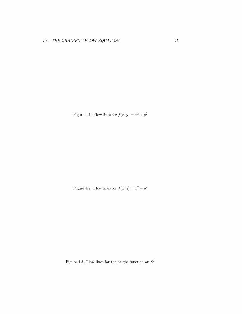
and therefore the gradient flow lines are (x, y) = (ae−2t, be−2t) for some fixed aand b. For any such line, y/x is a constant, so each lies in a line. In fact, it isthe open radial ray from the origin. See figure 4.1.
Example 4.3 Let M = R2 with the flat metric, and let f(x, y) = x2 − y2.Then it turns out that the gradient flow lines are (x, y) = (ae−2t, be2t) for somefixed a and b. For any such line, xy is a constant, so the gradient flow lines arehyperbolas of the form xy = c. See figure 4.2.
Example 4.4 Let M = S2 ⊂ R3 with the standard round metric, and letf(x, y, z) = z (the so-called “height function” defined by the embedding of S2
into R3). Then there are two critical points: one minimum at (0, 0,−1), andone maximum at (0, 0, 1). The flow lines are “lines of longitude”. See figure 4.2.
4.3. THE GRADIENT FLOW EQUATION 25
Figure 4.1: Flow lines for f(x, y) = x2 + y2
Figure 4.2: Flow lines for f(x, y) = x2 − y2
Figure 4.3: Flow lines for the height function on S2

26 CHAPTER 4. CRITICAL POINTS AND GRADIENT FLOW LINES
Figure 4.4: Flow lines for the height function on the torus
Example 4.5 Let T 2 be the torus in R3, embedded as follows:
(θ, φ) = (b cos(φ), (a+ b sin(φ)) cos(θ), (a+ b sin(φ)) sin(θ)
where 0 < b < a. The picture looks like a donut standing on its edge, as infigure 4.4. Again, take for f the “height function” z. Then there are four criticalpoints: (θ, φ) = (±π/2,±π/2), as you can check. The index for (π/2, π/2) is 2,the index for (π/2,−π/2) and (−π/2, π/2) is 1, and the index for (−π/2,−π/2)is 0.
There are two natural choices for a metric on T 2: either the metric inducedfrom the embedding from R3, or the flat metric defined by ds2 = dθ2 + dφ2.Although pictorially it may help to ponder the resulting gradient flow lines fromthe metric induced by R3 (these are the actual flows of steepest descent on aphysical donut), it is easier to calculate the flow lines when the flat metric isused. The flow lines can be described explicitly, or else you can verify that thereare flows with θ = ±π/2 for which θ is constant, and flows with φ = ±π/2 forwhich φ is constant. These flows give rise to two flows from the index 2 criticalpoint to one of the index 1 critical points, two flows from one index 1 criticalpoint to the other, and two flows from the lower index 1 critical point to theindex 0 critical point. The other flows are in a one-parameter family of flowswhich go from the index 2 critical point to the index 0 critical point.
Exercise 4.5 Work out the details of the above examples. Find the closed formsolutions to the gradient flow equations and find which critical points they con-nect to.
4.4 Basic properties of gradient flow lines
Lemma 4.5 The function f : M −→ R is nonincreasing along flow lines. f isstrictly decreasing along any flow line which does not contain a critical point.

4.4. BASIC PROPERTIES OF GRADIENT FLOW LINES 27
Proof: Let γ : (a, b) −→ M be a flow line. Consider the compositionf γ : (a, b) −→ R. Its derivative is given by
d
dtf(γ(t)) = 〈∇γ(t)(f),
dγ(t)dt
〉
= 〈∇γ(t)(f),−∇γ(t)(f)〉
= −∣∣∇γ(t)(f)
∣∣2 ≤ 0.
The only way this can be zero is if γ(t) is on a critical point of f . Inparticular, if γ(t) does not contain in its image a critical point of f , then f(γ(t))is strictly decreasing.
Remark 4.4 In the above proof, we showed
d
dtf(γ(t)) = −
∣∣∇γ(t)(f)∣∣2 .
We can also showd
dtf(γ(t)) = 〈∇γ(t)(f),
dγ(t)dt
〉
= 〈−dγ(t)dt
,dγ(t)dt
〉
= −∣∣∣∣dγ(t)dt
∣∣∣∣2 ≤ 0.
and this would also prove that f(γ(t)) is nonincreasing.
Remark 4.5 Now if γ(t) does contain a critical point p, then by example 4.1the flow must be a constant flow, and f(γ(t)) is constant on this flow.
Thus there are two kinds of flow lines: constant flows that stay at a criticalpoint, and flows that descend for all t, and do not contain a critical point.
Theorem 4.6 Suppose that M is a closed manifold. Then given any x ∈ Mthere is a unique flow line defined on entire real line
γx : R −→M
that satisfies the initial condition
γx(0) = x.
Furthermore the limits
limt→−∞
γx(t) and limt→+∞
γx(t)
converge to critical points of f . These are referred to as the starting and endingpoints of the flow γx.
The flow mapT : M × R −→M
defined by T (x, t) = γx(t) is smooth.

28 CHAPTER 4. CRITICAL POINTS AND GRADIENT FLOW LINES
Proof: Let x ∈M . By the existence and uniqueness of solutions to ordinarydifferential equations, there is an ε > 0 and a unique path
γx : (−ε, ε) −→M
satisfying the flow equation
dγx(t)dt
+∇γx(t)(f) = 0
for all |t| < ε, and the initial condition γx(0) = x. By the compactness of M wecan choose a uniform ε for all x ∈ M . Notice therefore that for |t| < ε we candefine a self map of M ,
γt : M −→M
by the formula γt(x) = γx(t). Notice that γ0 = id, the identity map. Byuniqueness it is clear that
γt+s = γt γsproviding that |t|, |s|, |t+ s| < ε. Among other things this implies that each γtis a diffeomorphism of M because γ−1
t = γ−t.Now suppose that |t| ≥ ε. Write t = k(ε/2) + r where k ∈ Z and |r| < ε/2.
If k ≥ 0 we defineγt = γ ε
2 γ ε
2 . . . γ ε
2 γr
where the map γ ε2
is repeated k times. If k < 0 then replace γ ε2
by γ−ε2
. Thusfor every t ∈ R we have a map γt : M −→ M satisfying γt γs = γt+s, andhence each γt is a diffeomorphism.
The curvesγx : R −→M
defined by γx(t) = γt(x) clearly satisfy the flow equations and the initial condi-tion γx(0) = x. This means that the gradient flow equations can be solved forall t ∈ R, and in particular, we will from now on require that gradient flow linesbe defined as functions γ : R −→ M instead of being defined only on an openinterval.
Now let γ be a flow line. Consider the composition f γ : R −→ R. By theFundamental Theorem of Calculus, if a < b, then
(f γ)(b)− (f γ)(a) =∫ b
a
d
dt(f γ)(t) dt.
Since M is compact f γ has bounded image, so the left side is bounded. ByLemma 4.5, d
dt (f γ) < 0. Therefore
limt→±∞
d
dt(f γ)(t) = 0.
By the proof of Lemma 4.5 we know that
0 = limt→±∞
d
dtf(γ(t)) = lim
t→±∞−∣∣∇γ(t)(f)
∣∣2 .

4.5. HEIGHT-PARAMETERIZED GRADIENT FLOW LINES 29
Let U be any union of small disjoint open balls around the critical points. Bythe compactness of M , M − U is compact, so |∇x(f)|2 has a minimum valueon M − U . Since M − U has no critical points, this minimum value is strictlypositive. But since the above limit is zero, we know that for sufficiently large |t|,γ(t) ∈ U . Since the balls are disjoint and γ(t) is continuous, there is a criticalpoint p so that for any open ball around p, γ(t) is in that ball for sufficientlylarge t. Therefore limt→∞ γ(t) exists and is equal to p; similarly, limt→−∞ γ(t)exists and is equal to a critical point.
The differentiability of the flow map T (x, t) = γx(t) with respect to t followsbecause γx(t) satisfies the differential equation. The differentiability of T withrespect to x follows from Peano’s theorem (the differentiable dependence of so-lutions to ODEs with respect to initial conditions). This is proved in Hartman’sbook on ODEs [?] in chapter V, Theorem 3.1.
4.5 Height-parameterized Gradient Flow Lines
Let γ(t) be a non-constant gradient flow line from p to q. Then by Lemma 4.5,we know that h(t) = f(γ(t)) is strictly decreasing, and in particular, is a diffeo-morphism from R to the open interval (f(q), f(p)). We can therefore considerthe smooth curve η(t) = γ(h−1(t)) from (f(q), f(p)) to M . Then it is easy tocheck that f(η(t)) = t. So γ and η have the same image, but the parameter inη represents height (that is, the value of f).
Exercise 4.6 Prove that f(η(t)) = t as claimed above.
We can also extend η to a continuous map from the closed interval [f(q), f(p)]to M by defining η(f(q)) = q and η(f(p)) = p.
Exercise 4.7 Prove that the extension of η to the closed interval [f(q), f(p)] iscontinuous.
Definition 4.7 If γ(t) is a non-constant gradient flow line for f , and h(t) =f(γ(t)), then
η(t) = γ(h−1(t)) : [f(q), f(p)] −→ R
is the height-reparameterization of γ, and such a curve is a height-parameterizedgradient flow of f .
Remark 4.6 This reparameterization of γ is a direction-reversing one, sinceh is strictly decreasing. This is to be expected since f(γ(t)) is decreasing butf(η(t) = t is increasing.
We now differentiate η.
Exercise 4.8 Proved
dtη(t) =
∇η(t)(f)∣∣∇η(t)(f)∣∣2

30 CHAPTER 4. CRITICAL POINTS AND GRADIENT FLOW LINES
Therefore, η(t) is the solution to another differential equation which may bedescribed as follows:
Lemma 4.8 Away fron the critical points of f , we may consider the vector field
X(x) =∇x(f)|∇x(f)|2
.
Then we define curves ζ : (s1, s2) −→M that satisfy
d
dtζ(t) = X(ζ(t))
Then ζ is a height-reparameterized flow line.
Proof: We insist that (s1, s2) be maximal. We then can show that ddtf(ζ(t)) =
1 as usual (do this now if you wish). Pick a number s ∈ (s1, s2), and consider thegradient flow line γ(t) so that γ(0) = ζ(s). We do the height-reparameterizationto γ to get a height-reparameterized curve η. Now η satisfies the same differ-ential equation as ζ, and η(f(ζ(s))) = ζ(s), so we translate the domain asfollows: η0(t) = η(t + f(ζ(s)) − s) satisfies the same differential equation as ζand η0(s) = ζ(s) so by the uniqueness of solutions to ODEs, η0 = ζ.
Therefore solutions to ddtζ(t) = X(ζ(t)) are precisely those that are height-
parameterized flows. Therefore X(x) and ∇(f(x)) have the same integral curves, although with
different parameterizations.

Chapter 5
The Classical Approach toMorse Theory
In the introduction (section 0.2), we mentioned that a Morse function on a closedmanifold produces a CW complex decomposition of the manifold, with a cell ofdimension λ for each critical point of index λ of f . In this chapter, we provethis statement up to homotopy. That is, we construct a homotopy equivalenceof the manifold to a CW complex of the kind just described. This is the originalapproach to Morse theory by Morse [?] and we follow the approach of Milnor[?] in this chapter.
Throughout this chapter, we will assume M is a closed manifold and f :M −→ R is a smooth Morse function. We will also consider the followingmanifolds (with boundary):
Ma = f−1(−∞, a] = x ∈M | f(x) ≤ a.
where a is any real number. If a is less than the minimum value of f , thenMa is the empty set. If a is larger than the maximum value of f , then Ma isM . The values of a in between will provide, up to homotopy, the necessary celldecomposition.
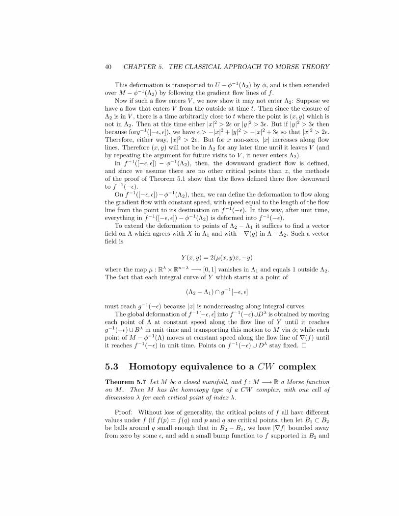
There are a number of technical details, but the intuition is simple: Let Mbe a surface embedded in R3, and f be the vertical coordinate z. We initiallylet a be less than the minimum value of f so that Ma = ∅, and graduallyincrease a (see Figure 5.1). This is analogous to gradually filling the surfacewith water, so that Ma is the part of the surface that is under water. Now if aincreases from a1 to a2 without passing through critical values, then Ma1 andMa2 are diffeomorphic (see Figure 5.2). But if, by increasing from a1 to a2, wepass through one critical point, then at that point the water may do somethingmore interesting. Up to homotopy, this turns out to be an attaching of a cell ofdimension λ, where λ is the index of the critical point (see Figure 5.3).
So as we pass critical points one by one, the manifold is created by suc-cessively attaching cells (up to homotopy type). This demonstrates that the
31

32 CHAPTER 5. THE CLASSICAL APPROACH TO MORSE THEORY
Figure 5.1: Ma for different values of a
Figure 5.2: Ma1 and Ma2 are diffeomorphic if there are no critical values be-tween a1 and a2.
Figure 5.3: When there is one critical value between a1 and a2, Ma2 is homotopyequivalent to Ma1 with a cell attached.

5.1. THE REGULAR INTERVAL THEOREM 33
manifold is homotopy equivalent to a CW complex of the type described above.In this chapter we prove the details of the above intuition. First we prove
that nothing happens if there is no critical point between two levels, using theresults of gradient flow lines from chapter 4. Then we show that if there is onecritical point between the two levels, the homotopy type changes by adding acell. We prove this via the Morse Lemma (Theorem 5.3), which studies thebehavior of f near a critical point. We conclude by producing the homotopyequivalence between the manifold and the CW complex, and giving some inter-esting applications to topology.
Exercise 5.1 Let M be a manifold and let f : M −→ R be a Morse function.Prove that f−1(a), the boundary of Ma, is a manifold if a is a regular valueof f .
5.1 The Regular Interval Theorem
We first show that if we increase Ma from Ma1 to Ma2 , and there are no criticalvalues between a1 and a2, then Ma1 and Ma2 are diffeomorphic.
The main point is the following theorem:
Theorem 5.1 (Regular interval theorem) Let f : M −→ [a, b] be a smoothmap on a compact Riemannian manifold with boundary. Suppose that f has nocritical points and that f(∂M) = a, b. Then there is a diffeomorphism
F : f−1(a)× [a, b] −→M
making the following diagram commute:
f−1(a)× [a, b] F−−−−→ M
proj.
y yf[a, b] −−−−→
=[a, b].
In particular all the level surfaces are diffeomorphic.
Proof: Since f has no critical points we may consider the vector field
X(x) =∇x(f)|∇x(f)|2
.
defined in Lemma 4.8. Let ηx(t) be a curve through x satisfying
d
dtηx(t) = X(ηx(t))
and f(ηx(t)) = t.Let I be a maximal interval on which ηx is defined. We wish to show that
I = [a, b]. First, since M is compact, f(ηx(I)) = I is bounded.

34 CHAPTER 5. THE CLASSICAL APPROACH TO MORSE THEORY
Let d = sup(I). Then by the compactness of M , there is a point x ∈ Mthat is a limit point of ηx(d − 1/n). Since η′x(t) = X(ηx(t)) is bounded, thislimit point is unique, and limt→d− ηx(t) = x. We can extend ηx to d by makingηx(d) = x.
Now limt→d η′x(t) = limt→dX(ηx(t)) → X(ηx(d)), and let v be this limit.
We will now show that η′x(d) = v. In particular, we will show that for everyε > 0, there exists a δ > 0 so that for all h with 0 < h < δ,∣∣∣∣ηx(d)− ηx(d− h)
h− v
∣∣∣∣ < ε.
Note that a coordinate chart is chosen near ηx(d) to allow the subtraction here.So let ε > 0 be given. By the definition of v, there exists a δ1 so that for all
w with 0 < h < δ1,|η′x(d− h)− v| < ε
By the fundamental theorem of calculus,
ηx(d− h)− ηx(d) =∫ d
d−hη′x(t) dt
ηx(d− h)− ηx(d) + vh =∫ d
d−h(η′x(t)− v) dt
|ηx(d− h)− ηx(d) + vh| ≤∫ d
d−h|η′x(t)− v| dt
≤∫ d
d−hε dt
≤ εh∣∣∣∣ηx(d− h)− ηx(d)h
+ v
∣∣∣∣ ≤ ε∣∣∣∣ηx(d− h)− ηx(d)−h
− v
∣∣∣∣ ≤ ε
Therefore η′x(d) = v, and since v = X(ηx(d)), the flow equation is satisfied byηx at d.
By maximality of I, d ∈ I. Similarly with c = inf(I), we see that c ∈ I.Therefore I is closed.
If ηx(s) 6∈ ∂M , then by the existence of solutions of ODEs, there is aninterval (s − ε, s + ε) around s on which ηx satisfies the differential equationη′x(t) = X(ηx(t)). Therefore ηx(c) and ηx(d) are in ∂M . Thus c = f(ηx(c)) andd = f(ηx(d)) may be either a or b. Since the derivative of f ηx is one, we seethat c = a and d = b. Therefore I = [a, b].
Since x ∈ M was arbitrary, and a ≤ f(x) ≤ b, we see that f(M) = [a, b].Furthermore, if x 6∈ ∂M , then by the existence of solutions to ODEs, as above,

5.1. THE REGULAR INTERVAL THEOREM 35
we have ηx defined in a small neighborhood of t = f(x), so that a < f(x) < b.Therefore f−1(a) and f−1(b) are unions of boundary components.
Define a mapF : f−1(a)× [a, b] −→M
by the formulaF (x, t) = ηx(t).
The differentiability of F follows from the same argument as in Theorem 4.6 toprove the differentiability of T , but with ηx instead of γx.
DefineG : M −→ f−1(a)× [a, b]
asG(x) = (ηx(a), f(x)).
The differentiability of G follows in the same way as the differentiability of F .We claim that F and G are inverses. To prove this, note that the integralcurves through x and ηx(t) are the same, that f(ηx(t)) = t and by uniquenessof solutions to ODEs, we have F (G(x)) = x and G(F (x, t)) = (x, t). This provesthat F is a diffeomorphism.
Corollary 5.2 Let M be a compact manifold, and f : M −→ R a smooth Morsefunction. Let a < b and suppose that f−1[a, b] ⊂M contains no critical points.Then Ma is diffeomorphic to M b. Furthermore, Ma is a deformation retract ofM b.
Proof: First we prove that Ma is a deformation retract of M b. By theregular interval theorem (Theorem 5.1), there is a natural diffeomorphism Ffrom f−1([a, b]) to f−1(a) × [a, b]. Since f−1(a) × a is a deformation retractof f−1(a)× [a, b], we see that f−1(a) is a deformation retract of f−1([a, b]). Wecan now paste this deformation retraction with the identity on Ma to obtainthe deformation retracton from Mb to Ma.
To prove that Ma is diffeomorphic to M b we apply the same principle, butwe need to be more careful to preserve smoothness during the patching process.
Since the set of critical points of f is a closed subset of the compact set M(and hence is compact), the set of critical values of f is compact. Thereforethere are real numbers c and d with c < d < a so that there are no criticalvalues in [c, b].
By Theorem 5.1 there is a natural diffeomorphism F from f−1([c, b]) tof−1(c)×[c, b], that maps f−1([c, a]) diffeomorphically onto f−1(c)×[c, a]. Thereis also a diffeomorphism H : f−1(c)× [c, b] −→ f−1(c)× [c, a], and we can insistthat it be the identity on f−1(c)× [c, d] (finding this function is an easy exercisein one-variable analysis, and in case you are interested, is listed as an exercisebelow). Thus
F−1 H F : f−1([c, b]) −→ f−1([c, a])
is a diffeomorphism that is the identity on f−1([c, d]), and thus we can patch ittogether with the identity on Md to create a diffeomorphism from Mb to Ma.

36 CHAPTER 5. THE CLASSICAL APPROACH TO MORSE THEORY
This corollary says that the topology of the submanifolds Ma does notchange with a ∈ R so long as a does not pass through a critical value.
Exercise 5.2 Fill in the detail of the proof of Corollary 5.2 that finds a dif-feomorphism H : f−1(c) × [c, b] −→ f−1(c) × [c, a] that is the identity onf−1(c)× [c, d].
5.2 Passing through a critical value
We now examine what happens to the topology of these submanifolds whenone does pass through a critical value. For this, we will need to understandthe function f in the neighborhood of a critical point. This is what the Morselemma provides us:
Theorem 5.3 (Morse Lemma) Let p be a nondegenerate critical point of in-dex λ of a smooth function f : M −→ R, where M is an n-dimensional manifold.Then there is a local coordinate system (x1, . . . , xn) in a neighborhood U of pwith xi(p) = 0 with respect to which
f(x1, . . . , xn) = f(p)−λ∑i=1
x2i +
n∑j=λ+1
x2j .
The proof given here is essentially that in Milnor’s famous book on Morsetheory [?].
Proof: Since this is a local theorem we might as well assume that f : Rn −→R with a critical point at the origin, p = 0. We may also assume without loss ofgenerality that f(0) = 0. Given any coordinate system for Rn we can thereforewrite
f(x1, . . . , xn) =n∑j=1
xjgj(x1, . . . , xn)
for (x1, . . . , xn) in a neighborhood of the origin. In this expression we have
gj(x1, . . . , xn) =∫ 1
0
∂f
∂xj(tx1, . . . , txn)dt.
Now since 0 is a critical point of f , each gj(0) = 0, and hence we may writeit in the form
gj(x1, . . . , xn) =n∑i=0
xihi,j(x1, . . . , xn).
Let φi,j = (hi,j + hj,i)/2. Hence we can combine these equations and write
f(x1, . . . , xn) =n∑
i,j=1
xixjφi,j(x1, . . . , xn)

5.2. PASSING THROUGH A CRITICAL VALUE 37
where (φi,j) is a symmetric matrix of functions. By doing a straightforwardcalculation one sees furthermore that the matrix
(φi,j(0)) =(
12
∂2f
∂xi∂xj(0))
and hence by the nondegeneracy assumption is nonsingular. From linear algebrawe know that symmetric matrices can be diagonalized. The Morse lemma willbe proved by going through the diagonalization process with the representationof f as
∑xixjφi,j .
Assume inductively that there is a neighborhood Uk of the origin and coor-dinates u1, . . . , un with respect to which
f = ±(u1)2 ± · · · ± (uk)2 +∑
i,j≥k+1
uiujψi,j(u1, . . . , un)
where (ψi,j) is a symmetric, n−k×n−k matrix of functions. By a linear changein the last n− k coordinates if necessary, we may assume that ψk+1,k+1(0) 6= 0.
Letσ(u1, . . . , un) =
√|ψk+1,k+1(u1, . . . , un)|
in perhaps a smaller neighborhood V ⊂ Uk of the origin. Now define newcoordinates
vi = ui for i 6= k + 1
and
vk+1(u1, . . . un) = σ(u1, . . . , un)
[uk+1 +
n∑i=k+2
uiψi,k+1(u1, . . . , un)ψk+1,k+1(u1, . . . , un)
].
The vi’s give a coordinate system in a sufficiently small neighborhood Uk+1 ofthe origin. Furthermore a direct calculation verifies that with respect to thiscoordinate system
f =k+1∑i=1
±(vi)2 +n∑
i,j=k+2
vivjθi,j(v1, . . . , vn)
where (θi,j) is a symmetric matrix of functions. This completes the inductivestep. The only remaining point in the theorem is to observe that the number ofnegative signs occuring in the expression for f as a sum and difference of squaresis equal to the number of negative eigenvalues (counted with multiplicity) ofHess0(f) which does not depend on the particular coordinate system used.
Remark 5.1 The Morse Lemma describes the behavior of the function f neara critical point, but it does not describe the behavior of the gradient flow lines.The reason for this is that the gradient depends on the Riemannian metric, andif we use the coordinate system given by the Morse Lemma, we do not know howthis metric behaves. See section 6.2 in chapter refch:cw.

38 CHAPTER 5. THE CLASSICAL APPROACH TO MORSE THEORY
Corollary 5.4 If M is a manifold and f : M −→ R is Morse, then the set ofcritical points of f is a discrete subset of M .
Proof: Suppose there were a sequence of critical points xn converging tosome point a ∈ M . Since df is a continuous one-form on M , we know that ais a critical point of f . Then apply the Morse Lemma above to a, which givesa formula for f in a neighborhood of a. But there are no critical points in thisneighborhood as can be seen directly by calculating df in these coordinates.This is a contradiction.
Exercise 5.3 Prove the converse of Exercise 5.1; that is, if M is a compactmanifold and f : M −→ R is a Morse function, and if a is not a regular valueof f , then f−1(a) is not a manifold.
Definition 5.5 Let f : M −→ [a, b] be a Morse function on a compact manifold.We say that f is admissible if ∂M = f−1(a)∪f−1(b), where a and b are regularvalues. This implies that each of f−1(a) and f−1(b) are unions of connectedcomponents of ∂M .
Theorem 5.6 Let f : M −→ R be an admissible Morse function on a compactmanifold. Suppose f has a unique critical point z of index λ. Say f(z) = c. Thenthere exists a λ - dimensional cell Dλ in the interior of M with Dλ ∩ f−1(a) =∂Dλ, and there is a deformation retraction of M onto f−1(a) ∪Dλ.
Proof: [Proof, following [?], with a few errors corrected] By replacing f byf(x) − c we can assume that f(z) = 0. Notice that by the regular intervaltheorem Theorem 5.1 it is sufficient to prove the theorem for the restriction off to the inverse image of any closed subinterval of [a, b] around c = 0.
Let (φ,U) be an chart around z with respect to which the Morse lemma issatisfied. Write Rn = Rλ×Rn−λ. φ maps U diffeomorphically onto an open setV ⊂ Rλ × Rn−λ, and
f φ−1(x, y) = −|x|2 + |y|2.
Notice that φ(z) = (0, 0). Put g(x, y) = −|x|2 + |y|2.We will use gradient flows, which depend on the metric on M . We choose
a metric for M by pulling back the flat metric on Rn by φ, and extending themetric arbitrarily to the rest of M . In this way, φ will be a local isometry, and
Dφ(u)(∇u(f)) = ∇v(g),
for any u ∈ U such that φ(u) = v ∈ V .Let 0 < δ < 1 be such that V contains Λ = Bλ(δ)×Bn−λ(δ) where
Bi(δ) = x ∈ Ri |n∑j=1
x2j ≤ δ
is the closed coordinate ball around the origin of radius δ.

5.2. PASSING THROUGH A CRITICAL VALUE 39
Let ε > 0 be small enough that√
4ε < δ, and let
cλ = Bλ(√ε)× 0 ⊂ V
and we define
Dλ = φ−1(cλ) ⊂M.
A deformation of f−1[−ε, ε] to f−1(ε) ∪ Dλ is made by patching togethertwo deformations. First consider the set
Λ1 = Bλ(√ε)×Bn−λ
(√2ε).
Consider the following figure for the case λ = 1, n = 2.
Note that inside Λ1, f(x, y) = −|x|2 + |y|2 > −ε+ |y|2 > −ε. Furthermore,since x ∈ Bλ (
√ε), we have that (x, 0) ∈ cλ.
In Λ1 ∩ g−1[ε, ε] a deformation is obtained by moving (x, y) at constantspeed along the interval joining (x, y) to the point (x, 0) ∈ g−1(−ε) ∪ Bλ, by(x, (1− t)y). This deformation then induces a deformation of φ−1(Λ1).
Outside the set
Λ2 = Bλ(√
2ε)×Bn−λ(√
3ε)
the deformation moves each point along the vector field −∇(g) so that it reachesg−1(−ε) in unit time. (The speed of each point is chosen to equal the length of itspath under the deformation.) See the following figure for a pictorial descriptionof this deformation.
40 CHAPTER 5. THE CLASSICAL APPROACH TO MORSE THEORY
This deformation is transported to U − φ−1(Λ2) by φ, and is then extendedover M − φ−1(Λ2) by following the gradient flow lines of f .
Now if such a flow enters V , we now show it may not enter Λ2: Suppose wehave a flow that enters V from the outside at time t. Then since the closure ofΛ2 is in V , there is a time arbitrarily close to t where the point is (x, y) which isnot in Λ2. Then at this time either |x|2 > 2ε or |y|2 > 3ε. But if |y|2 > 3ε thenbecause forg−1([−ε, ε]), we have ε > −|x|2 + |y|2 > −|x|2 + 3ε so that |x|2 > 2ε.Therefore, either way, |x|2 > 2ε. But for x non-zero, |x| increases along flowlines. Therefore (x, y) will not be in Λ2 for any later time until it leaves V (andby repeating the argument for future visits to V , it never enters Λ2).
In f−1([−ε, ε]) − φ−1(Λ2), then, the downward gradient flow is defined,and since we assume there are no other critical points than z, the methodsof the proof of Theorem 5.1 show that the flows defined there flow downwardto f−1(−ε).
On f−1([−ε, ε])−φ−1(Λ2), then, we can define the deformation to flow alongthe gradient flow with constant speed, with speed equal to the length of the flowline from the point to its destination on f−1(−ε). In this way, after unit time,everything in f−1([−ε, ε])− φ−1(Λ2) is deformed into f−1(−ε).
To extend the deformation to points of Λ2 − Λ1 it suffices to find a vectorfield on Λ which agrees with X in Λ1 and with −∇(g) in Λ−Λ2. Such a vectorfield is
Y (x, y) = 2(µ(x, y)x,−y)
where the map µ : Rλ×Rn−λ −→ [0, 1] vanishes in Λ1 and equals 1 outside Λ2.The fact that each integral curve of Y which starts at a point of
(Λ2 − Λ1) ∩ g−1[−ε, ε]
must reach g−1(−ε) because |x| is nondecreasing along integral curves.The global deformation of f−1[−ε, ε] into f−1(−ε)∪Dλ is obtained by moving
each point of Λ at constant speed along the flow line of Y until it reachesg−1(−ε)∪Bλ in unit time and transporting this motion to M via φ; while eachpoint of M − φ−1(Λ) moves at constant speed along the flow line of ∇(f) untilit reaches f−1(−ε) in unit time. Points on f−1(−ε) ∪Dλ stay fixed.
5.3 Homotopy equivalence to a CW complex
Theorem 5.7 Let M be a closed manifold, and f : M −→ R a Morse functionon M . Then M has the homotopy type of a CW complex, with one cell ofdimension λ for each critical point of index λ.
Proof: Without loss of generality, the critical points of f all have differentvalues under f (if f(p) = f(q) and p and q are critical points, then let B1 ⊂ B2
be balls around q small enough that in B2 − B1, we have |∇f | bounded awayfrom zero by some ε, and add a small bump function to f supported in B2 and

5.3. HOMOTOPY EQUIVALENCE TO A CW COMPLEX 41
constant in B1 whose gradient is bounded above by ε, and which does not raisethe value of f(q) high enough to reach another critical value of f).
Now let a0 < · · · < ak be a sequence of real numbers so that a0 is lessthan the minimum value of f , ak is greater than the maximum value of f , andbetween ai and ai+1 there is exactly one critical point. By Theorem 5.6 we havea homotopy equivalence hi between Mai+1 and Mai ∪ Dλi (where the unionis an attaching map as in a CW complex). By composing the hi’s, we obtaina homotopy equivalence from M = Mak to a union of disks attached by CWattaching maps.
Corollary 5.8 Given f : M −→ R as above there is a chain complex referredto as the Morse–Smale complex
. . . −→ Cλ∂λ−−−−→ Cλ−1 −→ . . .
∂1−−−−→ C0(5.1)
whose homology is H∗(M ; Z), where Cλ is the free abelian group generated bythe critical points of f of index λ.
Proof: This is the cellular chain complex coming from the CW complex inTheorem 5.7.
We can now prove some of the results promised in the introduction, thatrelate the topology of M to the numbers of critical points of f :
Corollary 5.9 (Morse’s Theorem) Let f : M −→ R be a C∞ function sothat all of its critical points are nondegenerate. Then the Euler characteristicχ(M) can be computed by the following formula:
χ(M) =∑
(−1)ici(f)
where ci(f) is the number of critical points of f having index i.
Proof: The Euler characteristic χ(M) can be computed as the alternatingsum of the ranks of the chain groups of any CW decomposition of M .
Corollary 5.10 (Weak Morse Inequalities) Let cp be the number of criticalpoints of index p and let βp be the rank of the homology group Hp(M). Then
βp ≤ cp.
Proof: The chain group Cp ⊗ R generated by the cp cells of dimension p isa vector space of dimension cp. The group of cycles is of dimension at most cp.After quotienting by the boundaries, we see that Hp(M ; R) is a vector space ofdimension at most cp.
42 CHAPTER 5. THE CLASSICAL APPROACH TO MORSE THEORY
Corollary 5.11 (Strong Morse Inequalities) Let M , f , ci(f), and bi(M)be as above. Then for all natural numbers i,
i∑k=0
(−1)i−kci(f) ≥i∑
k=0
(−1)i−kbi(M).
Proof: The proof is similar except we take a closer look at the boundaries.Tensoring the chains with R, so that we write Vk = Ck⊗R, we get the followingchain complex of vector spaces:
. . . −→ Vi∂i−−−−→ Vi−1 −→ . . .
∂1−−−−→ V0
We write Vk as Im(∂k+1)⊕Hk(M ; R)⊕ (Vk/ ker(∂k)) and note that Im(∂k+1)is of the same dimension as Vk+1/ ker(∂k+1). Thus if we define dk to be thedimension of Vk/ ker(∂k), we have
ck = dk+1 + bk + dk
and applying the alternating sum above we get
i∑k=0
(−1)i−kci(f) = di+1 +i∑
k=0
(−1)i−kbi(M)
(where here we need that d0 = 0). This proves the strong Morse inequalities. To see that the strong Morse inequalities prove the weak Morse inequalities,
write down the strong Morse inequality for i and for i+1, and subtract the twoinequalities. To see that the strong Morse inequalities imply Morse’s theorem,apply the strong Morse inequality for i and for i + 1 for i larger than thedimension of the manifold M , noting that cj = 0 and bj = 0 for all j > dim(M).
It is instructive to work out the following:
Exercise 5.4 Show that the strong Morse inequalities is “strictly stronger” thanthe weak Morse inequalities together with Morse’s theorem. What I mean is:given the n+1-tuple of natural numbers (b0, . . . , bn), we can find another n+1-tuple of natural numbers (c0, . . . , cn) so that these numbers satisfy the weakMorse inequality and the Morse theorem but not the strong Morse inequalties.
A typical application of these result is to use homology calculations to deducecritical point data. For example we have the following.
Application 5.12 Every Morse function on the complex projective space
f : CPn −→ R
has at least one critical point in every even dimension ≤ 2n.
The following is a historically important application of Morse theory, due toReeb, that follows from the techniques we have mentioned so far.

5.3. HOMOTOPY EQUIVALENCE TO A CW COMPLEX 43
Application 5.13 Let Mn be a closed manifold admitting a Morse function
f : M −→ R
with only two critical points. Then M is homeomorphic to the sphere Sn.
Remark 5.2 This theorem does not imply that M is diffeomorphic to Sn. In[?] Milnor found an example of a manifold that is homeomorphic, but not dif-feomorphic to S7. Indeed he proved that there are 28 distinct differentiablestructures on S7! Milnor actually used this fact to prove that the manifolds heconstructed were homeomorphic to S7.
Proof: [Proof of Theorem 5.13] Let S and N be the critical points. By thecompactness of M we may assume that S is a minimum and N is a maximum.(Think of them as the eventual south and north poles of the sphere.) Let f(S) =t0 and f(N) = t1. By the Morse lemma there are coordinates (x1, . . . , xn) in aneighborhood U+ of N with respect to which f has the form
−x21 + · · ·+−x2
n + t1.
Therefore there is a b < t1 so that if we let D+ = f−1[b, t1] then there is adiffeomorphism
D+∼= Dn
with ∂D+ = f−1(b) ∼= Sn−1. Repeating this process with the minimum pointP we obtain a point a > t0 and a diffeomorphism of the space D− = f−1[t1, a],
D− ∼= Dn
with ∂D− = f−1(a) ∼= Sn−1. By Theorem 5.1 we have that
f−1[a, b] ∼= f−1(a)× [a, b] ∼= Sn−1 × [a, b].
Hence we have a decomposition of the manifold
M = f−1[t0, t1] = f−1[t0, a] ∪ f−1[a, b] ∪ f−1[b, t1]∼= Dn ∪ Sn−1 × [a, b] ∪Dn
where the attaching maps are along homeomorphisms of Sn−1. We leave it asan exercise to now construct a homeomorphism from this manifold to Sn.
Exercise 5.5 Finish the proof of Theorem 5.13 by showing that the resultingspace
Dn ∪ Sn−1 × [a, b] ∪Dn
is homeomorphic to Sn. Hint: Start by embedding one Dn into Sn, then embedSn−1 × [a, b] into Sn to match the first embedding, then to put the last Dn in,you must think of Dn as the cone on Sn−1. This last part is why the proof doesnot prove that this is diffeomorphic to Sn.
44 CHAPTER 5. THE CLASSICAL APPROACH TO MORSE THEORY
In general, there are many applications of this work to the problem of clas-sifying manifolds of dimensions 5 and higher, leading to the h-cobordism theo-rem and the s-cobordism theorem, and surgery theory. There are many booksthat describe these developments of the 1960s and 1970s, the old classics beingMilnor’s book on the h-cobordism theorem, which hides the Morse theoreticmotivation [?], Wall’s book on surgery theory [?], and Browder’s book [?] thatcovers the same topics but is more readable because he restricts to the simply-connected case. More friendly introductions to the subject, recommended forstudents, are [?], [?] and [?].

Part II
Spaces of gradient flows
45


Chapter 6
Morse theory usingunstable manifolds
The previous chapter described how any closed manifold M is homotopy equiv-alent to a CW complex given by a Morse function f . It would be nice to showmore explicitly where the cells of the CW complex come from. In particular,it would be nice if we could describe the manifold as a CW complex directly,instead of referring to homotopy equivalences.
This is actually explained in chapter 10, but in this chapter we set the stageby decomposing M into open disks. Each of these open disks comes from acritical point of the function f .
6.1 Stable and unstable manifolds of a criticalpoint
As before, for any point x ∈ M , let γx(t) be the flow line through x, i.e. itsatisfies the differential equation
d
dtγ = −∇γ(f)
with the initial condition γ(0) = x. We know by Theorem 4.6 that γx(t) tendsto critical points of f as t→ ±∞. So for any critical point a of f we define thestable manifold W s(a) and the unstable manifold Wu(a) as follows:
Definition 6.1 Let M be a manifold, and f a smooth function on M . Let a bea critical point for f . We define the two subsets of M :
W s(a) = x ∈M : limt→+∞
γx(t) = a
Wu(a) = x ∈M : limt→−∞
γx(t) = a.
and call W s(a) the stable manifold of a and Wu(a) the unstable manifold of a.
47

48 CHAPTER 6. MORSE THEORY USING UNSTABLE MANIFOLDS
Figure 6.1: The stable and unstable manifolds of a critical point.
In other words, W s(a) is the set of points on M that flow down to a, andWu(a) is the set of points on M that would flow “up” to a if the gradient flowwere reversed. The use of the term “manifold” is justified by the stable manifoldtheorem:
Theorem 6.2 (Stable Manifold Theorem) Let M be an n-dimensional man-ifold, and f : M −→ R a Morse function. Let a be a critical point of f of indexλ. Then Wu(a) and W s(a) are smooth submanifolds diffeomorphic to the opendisks Dλ and Dn−λ, respectively.
This will be proved in Section 6.3 below for a large class of metrics (thoughit is in general true for all metrics).
Proposition 6.3 If M is a compact manifold with Riemannian metric g, andf : M −→ R is a Morse function, then
M =⋃a
Wu(a)
is a partition of M into disjoint sets, where the union is taken over all criticalpoints a of f .
Proof: The fact that the union of the Wu(a) is M comes from the fact thatevery point of M lies on a flow line γ, and we can always find limt→−∞ γ(t).
The fact that the Wu(a) and Wu(b) are disjoint when a 6= b is due to thefact that γ is unique.
Exercise 6.1 Find the unstable manifolds for each critical point in Exam-ple 4.4.
Exercise 6.2 Consider the contour drawing of a Morse function f shown inFigure 6.2. Imagine that the domain is S2, and the contour drawing illustratesa coordinate patch of S2 that contains all critical points of f except for one

6.1. STABLE AND UNSTABLE MANIFOLDS OF A CRITICAL POINT 49
Figure 6.2: A contour drawing of a Morse function
minimum. Copy the contour drawing, and on this drawing, sketch the unstablemanifolds for each critical point.
Assume that there are no other critical points except the minimum and thosethat are visually apparent by the contour drawing. Assume also that the met-ric in this coordinate patch is the flat Euclidean metric corresponding to thecoordinates, so that the contour drawing may be viewed as on a region in R2.
Exercise 6.3 Find the unstable manifolds for each critical point in Exam-ple 4.5.
From these exercises you can see that this decomposition of M makes Mlook like a CW complex, with one cell of dimension λ for each critical point ofindex λ. The torus example is problematic because an edge gets attached tothe middle of another edge, but consider the following fix:
Exercise 6.4 Consider the torus in R3 as before, but with a slight perturbation.That is, tilt the torus by pulling it down slightly toward its hole, so that it is notstanding on its outside edge, as in Figure 6.4. Find the unstable manifolds foreach critical point here.
The point is that with this example, we have a decomposition of M intocells, with a cell of dimension λ for each critical point of index λ. These areessentially the cells Dλ in Theorem 5.6.
The disks appearing in this result and those appearing in Theorem 5.6 arerelated in the following way. Suppose that [t0, t1] ⊂ R has the property thatf−1([t0, t1]) ⊂ M has precisely one critical point a of index λ with f(a) =c ∈ (t0, t1). Then by Theorem 5.6 there is a disk Dλ ⊂ M t1 and a homotopyequivalence
M t1 'M t0 ∪Dλ.

50 CHAPTER 6. MORSE THEORY USING UNSTABLE MANIFOLDS
Now note that Wu(a) ∩ f−1([t0, t1]) is, under a Euclidean metric definedby the Morse coordinate chart, equal to the Dλ mentioned in the proof ofTheorem 5.6.
[ See Chap 3.7; there is more of a statement there about diffeomorphismsthat bring Wu(a) ∩ f−1([t0, t1]) to Dλ. Or: in case of nice metric Also, draw apicture. ]
This strengthening of Theorem 5.7 makes it intuitively clear why the Morseequality (Theorem 5.9) and the Weak Morse inequalities (Corollary 5.10) hold.In addition, the Strong Morse inequalities (Corollary 5.11) also follow quickly.
There are several problems: first, we need to prove the Stable manifoldtheorem. Next, we need to prove that this decomposition into open cells isactually a CW complex. Now, a CW complex is described as a collection ofclosed disks, where the boundaries of these closed disks are identified with pointsthat lie in other disks, via functions called attaching maps. So we need to turnthe open disks Wu(a) into closed disks, and describe how they are attached.
As we saw in the first torus exercise above, it does not actually alwayswork. There is a condition (called the Morse–Smale condition) under whichthis program works. We will describe this condition in section 7. Under thiscondition, we will see in Chapter 10 how to view M as a CW complex.
At this stage, we should view this as roughly a CW complex decomposition,but with open disks instead of closed disks. These disks and other related spaceswill play a major role in the next several chapters.
We will then study the attaching maps for the CW complex decompositionin some detail, using framed cobordism. This allows us to find more topologicalinformation about M than is given in the Morse inequalities. For instance, itallows us to compute the homology of M explicitly.

6.2. NICE METRICS 51
6.2 Nice metrics
In chapter 5, we proved the Morse Lemma (Theorem 5.3), which says thatlocally, around any nondegenerate critical point, we can choose a coordinatechart so that
f(x1, . . . , xn) = f(p)−λ∑i=1
x2i +
n∑j=λ+1
x2j . (6.1)
In other words, we have a local explicit formula for f around a critical point,no matter what f is, as long as the critical point is non-degenerate.
What does the gradient vector field look like around such a critical point?Based on the above equation (6.1), you might expect the gradient to be this:
∇(f) = (−2x1, . . . ,−2xλ, 2xλ+1, . . . , 2xn) (6.2)
But because the metric is not described, it is possible (even likely) that thegradient vector field is not this at all. Recall that the gradient is obtained byg(v,∇(f)) = df(v) (see the discussion at the beginning of chapter 4, especiallyExercises 4.3 and 4.4).
Since we are dealing with gradient vector fields, and their corresponding flowlines, it would make sense for us to want to choose coordinates to standardize thegradient vector field so that equation (6.2) is true, rather than equation (6.1).This is especially the case, since if equation (6.2) is true, then the gradient flowequation
d
dtγ(t) = −∇γ(t)(f)
would take the form (if we write γ(t) = (x1(t), . . . , xn(t))):
x1 = 2x1
...xλ = 2xλ
xλ+1 = −2xλ+1
...xn = −2xn
which is easily solved since each equation only deals with one variable.If the metric is anything else, we might still hope to diagonalize this sys-
tem of differential equations, choosing coordinates (x1, . . . , xn) so that γ(t) =−∇γ(t)(f) looks like
xi = cixi (6.3)
for some non-zero real constants c1, . . . , cn. Then the ci would be negatives ofthe eigenvalues of the Hessian of f at the critical point, and the correspondingeigenvectors would be the standard basis vectors ∂/∂xi in this coordinate chart.
52 CHAPTER 6. MORSE THEORY USING UNSTABLE MANIFOLDS
Unfortunately, it is in general impossible to choose coordinates so that (6.3)holds, as the following exercises show:
Exercise 6.5 Solve the system of differential equations (6.3).
Exercise 6.6 Solve the system of differential equations
x = 2x (6.4)y = −y (6.5)z = z + xy (6.6)
(6.7)
and show that there is no change of coordinates that transform it into the form(6.3).
Exercise 6.7 Let f(x, y, z) = x2 − y2 + z2. Find a metric g(x, y, z) on aneighborhood of (0, 0, 0) ∈ R3 so that the gradient flow equations near the originare as in equation (6.7). Hence prove that it is in general impossible to choosecoordinates so that the gradient flow equations look like equation (6.3) in aneighborhood of the critical point. Note that the metric must be symmetric andpositive definite in the neighborhood.
Note that in this exercise, what goes wrong is a kind of “resonance” phe-nomenon that occurs in ordinary differential equations when two eigenvaluesare the same. By analogy, we would expect this kind of problem to be rare, andwe might hope that for most situations, we can choose coordinates to put thegradient flow equations in the standard form of equation (6.3), but to addressthis will take us rather far afield (see [?]).
Instead, we choose to follow Hutchings [?] to modify the metric to the stan-dard metric so that equation (6.1) gives rise to the gradient in equation (6.2),which in turn gives rise to the gradient flow equations in equation (6.3).
This motivates the following definition, due to Hutchings [?]:
Definition 6.4 Let M be a manifold and f be a Morse function. A metricis said to be nice if there exist coordinate neighborhoods around each criticalpoint of f so that for each such neighborhood there are non-zero real numbersc1, . . . , cn so that the gradient flow equations are
xi = cixi,
as in (6.3).
Proposition 6.5 Let M be a compact manifold and f a Morse function. Thereexists a nice metric on (M,f). In fact, these are dense in the L2 space ofmetrics.
6.3. THE PROOF OF THE STABLE/UNSTABLE MANIFOLD THEOREM53
Proof: Let g0 be any smooth metric onM . Consider the set of critical pointsof f . Apply the Morse lemma (Lemma 5.3), to find nonoverlapping coordinateneighborhoods of each critical point of f in M , each with coordinates x1, . . . , xnso that the Morse function in each neighborhood is
f(x1, . . . , xn) = f(p)−λ∑i=1
x2i +
n∑j=λ+1
x2j .
For each critical point a of f , let Ua be the coordinate neighborhood givenby the Morse lemma, let B1 be a coordinate ball around a that is completelyinside Ua, and let B2 be another coordinate ball around a of smaller radius thanB1. (By coordinate ball I mean the set whose coordinates (x1, . . . , xn) satisfyx2
1 + · · ·+ x2n < r for some r.)
Let φ : Ua −→ R be a smooth function so that φ is 1 on B2 and 0 outsideB1. Let gE be the standard Euclidean metric with respect to thex1, . . . , xncoordinates. Define g to be
g = g0(x)(1− φ(x)) + gE(x)φ(x).
Since the set of symmetric positive definite bilinear forms is a convex set, thisconvex linear combination of the two metrics will be a metric on Ua. Extendg by setting it equal to g0 on the rest of M . Then g is a metric for which a isnice.
Now proceed inductively through the other critical points of M . This createsa metric g so that there is a coordinate neighborhood metric ball B around eachcritical point where both f and the metric are in a standard form. Then thegradient flow equation
dγ
dt= ∇γ(f)
looks like equation (6.3).By taking B2 smaller and smaller, we see that the difference between g and
g0 is supported on an arbitrarily small set, and by the boundedness of the metricon M , we know that this difference is arbitrarily small in L2.
6.3 The proof of the stable/unstable manifoldtheorem
We now prove the Stable manifold theorem for nice metrics:
Theorem 2 (Stable Manifold Theorem) Let M be an n-dimensional man-ifold, with nice metric g, and f : M −→ R a Morse function. Let a be acritical point of f of index λ. Then Wu(a) and W s(a) are smooth submanifoldsdiffeomorphic to the open disks Dλ and Dn−λ, respectively.
Remark 6.1 This theorem is still true if the metric g is not nice, but to provethis would take too long and we don’t need it in this generality. Curious readerscan see [?] for the proof.

54 CHAPTER 6. MORSE THEORY USING UNSTABLE MANIFOLDS
Proof: [Proof of the Stable Manifold Theorem] If g is a nice metric, then thereis a coordinate neighborhood B around each critical point where the gradientflow equations are
dγidt
= ciγi(t)
where γi(t) is the i-th coordinate of γ. Note that the ci are the negatives ofeigenvalues of the Hessian, corresponding to the directions given by the stan-dard basis in the coordinate chart. Reorder the coordinates so that the first λeigenvalues are the negative ones (so that the first λ values of ci are positive).
Then explicitly,
γi(t) =
γi(0)e|ci|t, i ≤ λ
γi(0)e−|ci|t, i > λ(6.8)
inside B.We prove the theorem for W s(a). The proof for Wu(a) is exactly analogous,
and besides, it follows from the W s(a) case, applied to the function −f . Wewill first prove that W s(a) is smooth in a small neighborhood of a.
Let W0 be the subset of B consisting of those points where x1 = x2 = · · · =xλ = 0. Then from the explicit solution (6.8), we see that W0 ⊂W s(a).
Now W0 is an open disk of dimension n − λ centered on a, and hence is amanifold, and is furthermore a submanifold of M .
Recall from Theorem 4.6 that the flow map defined as
T : M × R −→M
T (x, t) = γx(t)
is smooth. Apply this flow backward in time by some time t: define Wt =T (W0,−t). This will be diffeomorphic to W0 and a subset of W s(a). As t goesto infinity, we span a larger and larger subset of W s(a).
Let x ∈ W s(a), and γ the corresponding gradient flow line with γ(0) = x.Since limt→∞ γ(t) = a, we know that for some t0 > 0, γ(t) ∈ B for all t ≥ t0. Iwill now show that γ(t0) ∈W0.
Suppose γ(t0) 6∈ W0. The translated flow η(t) = γ(t+ t0) is a gradient flowline, with the property that η(0) 6∈ W0, and η(t) ∈ B for all t > 0. Then forsome coordinate i > λ, ηi(0) 6= 0. By the explicit solution (6.8), ηi(t) will growindefinitely, so that eventually η (and hence γ) leaves the coordinate ball B.This is a contradiction. Therefore, γ(t0) ∈W0.
Since every element of W s(a), when flowed forward, eventually is in W0, weknow that ∪tWt = W s(a).
Let ψ : [0, 1) −→ R be a smooth monotonic function with ψ(0) = 0 andlimt→1 ψ(t) = +∞. Using |x| as
√x2
1 + · · ·+ x2n, and r0 as the radius of the
coordinate ball B, we see that T (x, ψ(|x|/r0)) maps W0 diffeomorphically ontoW s(a). Recall that W0 is a submanifold of M which is a disk of dimensionn− λ. Therefore, W s(a) is a submanifold of M and diffeomorphic to Dn−λ.

6.4. STRUCTURE OF F RESTRICTED TO STABLE/UNSTABLE MANIFOLDS55
Exercise 6.8 Prove the Stable Manifold Theorem (Theorem 2) for the unstablemanifold Wu(a), without applying the theorem to stable manifolds of −f . In-stead, carefully go through the proof for W s(a) and write out the correspondingproof that would work for Wu(a).
Proposition 6.6 The tangent space of W s(a) at a is the positive eigenspace ofthe Hessian of f at a. Similarly, the tangent space of Wu(a) at a is the negativeeigenspace of the Hessian of f at a.
Proof: Again, we are assuming the metric is nice, but this is unnecessary.Now W s(a) is a smooth submanifold of M , so its tangent space at a is
well-defined. Define W0 as in the previous proof, as
(x1, . . . , xn) | x1 = · · · = xλ = 0.
The tangent space to W0 is therefore the span of ∂/∂xi for i = λ+ 1 to n. Thisis the positive eigenspace of the Hessian.
On the other hand W0 ⊂W s(a), and since they are of the same dimension,W0 is an open neighborhood of a in W s(a). Therefore W0 and W s(a) have thesame tangent space at a.
The proof for Wu(a) can be done similarly, or if you wish, you may use theresult for W s(a) on −f .
6.4 Structure of f restricted to stable/unstablemanifolds
Let a be a critical point of f . Let us consider the function f restricted to Wu(a).Since Wu(a) is defined to be the set of points which in some sense lie “below” aon gradient flow lines, we expect a to be a maximum of f on Wu(a), and levelsets to be spheres around a.
Theorem 6.7 Let (M, g) be a Riemannian manifold and f : M −→ R a Morsefunction. Let a be a critical point of f . Let h : Wu(a) −→ R be the restrictionof f to Wu(a). Then a is the unique critical point of h, and it is the absolutemaximum. If ε > 0 is small enough, and f(a) − ε < c < f(a), then h−1(c) isdiffeomorphic to a λ− 1 dimensional sphere in Wu(a) around a.
Similarly, let j : W s(a) −→ R be the restriction of f to W s(a). Then a isthe unique critical point of j, and it is the absolute minimum. If ε > 0 is smallenough, and f(a) < c < f(a) + ε, then j−1(c) is diffeomorphic to a n − λ − 1dimensional sphere in W s(a) around a.
Proof: We will prove this for Wu(a), and the result for W s(a) is the sameusing −f instead of f .
Let x ∈ Wu(a), and x 6= a. Let γ(t) be the unique gradient flow line withγ(0) = x. Since x ∈Wu(a), we have that limt→−∞ γ(t) = a.

56 CHAPTER 6. MORSE THEORY USING UNSTABLE MANIFOLDS
According to Lemma 4.5, f(γ(t)) is strictly decreasing. By the continuityof f , limt→−∞ f(γ(t)) = f(a). So f(a) > f(x). Therefore, a is the absolutemaximum of h.
Now, γ(t) ∈ Wu(a) for all t, so γ′(0) ∈ TxWu(a). Since f(γ(t)) is strictly
decreasing, γ′(0) 6= 0 (if it were, ddtf(γ(t)) = ∇(f) · γ′(0) would be zero). By
the gradient flow equation γ′(t) = −∇γ(t)(f), the −∇x(f) 6= 0. Therefore, x isnot a critical point of h. Since x was arbitrary, except for not equalling a, thereare no critical points of h except for a.
Now we consider the Hessian of h at a. Find a coordinate chart of Maround a so that Wu(a) is given by the equations xλ+1 = · · · = xn = 0. Bythe invariance of the Hessian under coordinate change (Proposition 4.1), theHessian of f can be computed in such a coordinate chart. Since TaWu(a) is thenegative eigenspace of the Hessian of f (Proposition 6.6) we conclude that thematrix (
∂2f
∂xi∂xj
)ij
is negative definite. Since Wu(a) is given by setting xλ+1, . . . , xn to be constant(in fact, zero), we see that for i, j ≤ λ, this matrix is the same as(
∂2h
∂xi∂xj
)ij
.
Therefore the Hessian of h at a is negative definite. In particular, a is a non-degenerate critical point of h, and h is Morse.
We now consider the preimages h−1(c).For this, we use the Morse Lemma (Theorem 5.3) applied to h on the man-
ifold Wu(a). The Morse Lemma states that there exist a coordinate neighbor-hood U around a with coordinates x1, . . . , xλ on Wu(a) so that
h(x1, . . . , xλ) = f(a)− x21 − · · · − x2
λ.
Let ε > 0 be given so that the ball
B = (x1, . . . , xλ)|x21 + · · ·+ x2
λ < ε
is contained in U . Within this ball it is clear that the preimages h−1(c) (whenf(a)− ε < c < f(a)) are coordinate spheres around a. We will now verify thatthere are no other parts to h−1(c) which are outside B.
Suppose x ∈ Wu(a), and x 6∈ B. As earlier in the proof, let γ(t) be thegradient flow with γ(0) = x. As before, limt→−∞ γ(t) = a. But B is an openset around U . Therefore, for some t < 0, γ(t) ∈ B. Since x = γ(0) is not inB, the generalized Jordan curve theorem says that there exists some T < 0 forwhich γ(T ) is on the boundary of B. Since f(γ(t)) is strictly decreasing,
f(x) = f(γ(0)) < f(γ(T )) = f(a)− ε.
So f(x) < f(a) − ε. Therefore, if f(a) − ε < c < f(a), then h−1(c) is a susbetof B, and is therefore the coordinate spheres we found earlier.

Chapter 7
Morse–Smale functions:intersecting stable andunstable manifolds
7.1 The Morse–Smale condition
Consider Exercise 6.3. One of the edges did not attach to vertices, but to themidpoint of another edge. In Exercise 6.4, a perturbation of this situation, thisproblem is fixed, and both edges end at the bottom vertex. This indicates thatit is not enough that f be Morse for the unstable manifold picture to work well.We need a further transversality condition, which we define now.
Definition 7.1 Suppose f : M −→ R is a Morse function that satisfies theextra condition that for any two critical points a and b the unstable and stablemanifolds Wu(a) and W s(b) intersect transversally. This is the Morse–Smalecondition, and if f satisfies this condition, we call f a Morse–Smale function.
Smale [?] showed that Morse–Smale functions exist. More specifically, givena metric g and function f : M −→ R, there exists another metric g′ and anotherfunction f ′ : M −→ R so that f ′ is Morse–Smale with respect to g′. His proofalso demonstrates that f and f ′ and g and g′ can be made arbitrarily close toeach other. Hence the set of configurations of functions and metrics so that thefunctions are Morse–Smale with respect to that metric is dense.
Actually, more is true: if f is Morse, then for an open, dense set of metricsg, f is Morse–Smale. This can be proved using the same techniques that areused in the proofs in Smale’s paper. We will sketch out a proof at the end ofthis chapter that the set of such metrics is dense. In the meantime we will firststudy some properties of Morse–Smale functions.
Exercise 7.1 Show that the example in Exercise 6.4 is Morse–Smale, and theexample in Exercise 4.5 is not.
57
58CHAPTER 7. MORSE–SMALE FUNCTIONS: INTERSECTING STABLE AND UNSTABLE MANIFOLDS
Exercise 7.2 Suppose f is Morse (not necessarily Morse–Smale) and supposeb is a critical point of f . Do Wu(b) and W s(b) always intersect transversally?
7.2 Intersections of stable and unstable mani-folds: W (a, b)
The main purpose of the Morse–Smale condition is that it allows us to see howstable and unstable manifolds of different critical points intersect. For everypair of critical points a and b, let
W (a, b) = Wu(a) ∩W s(b).
W (a, b) is the space of all points in M that lie on flow lines starting from a andending at b.
Proposition 7.2 Let (M, g) be a Riemannian manifold of dimension n, letf : M −→ R be Morse–Smale, and a and b be two critical points of f . ThenW (a, b) is a smooth manifold of dimension
a)− b).
Proof: If f is Morse–Smale, then Wu(a) and W s(b) intersect transversally.So by Theorem 3.5, the intersection Wu(a) ∩W s(b) = W (a, b) is a manifold ofdimension dim(Wu(a)) + dim(W s(b))− n = a) + (n− b))− n = a)− b).
Corollary 7.3 Let f : M −→ R be a Morse–Smale function, and let a and bbe two distinct critical points of f . If a) ≤ b), then W (a, b) = ∅.
Proof: If a) < b), then the previous proposition shows that W (a, b) is amanifold of negative dimension, so it must be empty.
If a) = b), then similarly W (a, b) must be a manifold of dimension 0, butsince the gradient flow acts freely on elements of W (a, b), the dimension ofW (a, b) must be at least one. Therefore it must be empty.
Definition 7.4 We refer to the number
a)− b)
as the relative index of a and b.
Exercise 7.3 Find W (a, b) for each pair of critical points a and b for Exer-cise 6.4.
Exercise 7.4 Suppose a and b are critical points of f and a 6= b. Are a and bin W (a, b)? If there are other critical points of f , is it possible that these are inW (a, b)? Now consider the case a = b. What is W (a, b)?

7.3. MORSE–SMALE MODULI SPACES: W (A,B)T 59
7.3 Morse–Smale moduli spaces: W (a, b)t
The fundamental object of study will not usually be W (a, b), but a particular“horizontal” slice. If we view the gradient flow as an action of R on W (a, b),then we can study the orbit space (called the Moduli space) W (a, b)/R. Forgood intuition and for practical considerations it is useful to instead pick out arepresentative of each R orbit in W (a, b). One way to do this is to select a realnumber t between a and b and pick out the representative in f−1(t). This isthe approach used in our first definition of the moduli space (there will be otherequivalent definitions soon).
Definition 7.5 Pick a value t ∈ R between f(a) and f(b), and let W (a, b)t tobe the set W (a, b) ∩ f−1(t).
Proposition 7.6 If a and b are distinct critical points of f , then W (a, b)t is asmooth submanifold of M .
Proof: First, we see that f |W (a,b) : W (a, b) −→ R is transverse to the pointt ⊂ R. This is because for any point x ∈ W (a, b) so that f(x) = t, ∇x(f) isnot zero, and so neither is dfx(∇x(f)) = ‖∇x(f)‖2. Therefore f |W (a,b) t t.
Therefore, we may apply Theorem 3.5, and get that(f |W (a,b)
)−1 (t) =W (a, b)t is a submanifold of W (a, b) of codimension one.
Proposition 7.7 Let a and b be distinct critical points of f . The function
φ : W (a, b)t × R −→W (a, b)
defined byφ(p, s) = Ts(p)
is a diffeomorphism.
Proof: We begin by proving φ is onto. Let x ∈ W (a, b). Let γ be the flowline that has γ(0) = x. Since limt→∞ f(γ(t)) = f(b) and limt→−∞ f(γ(t)) =f(a), by continuity we have that for some s, f(γ(−s)) = t. Then γ(−s) = pand Ts(p) = x.
Now to show φ is one-to-one, suppose x = φ(p1, s1) = φ(p2, s2). ThenT−s1(x) = p1 and T−s2(x) = p2, meaning that the unique flow line γ withγ(0) = x also has γ(s1) = p1 and γ(s2) = p2. Since f(p1) = t = f(p2), andddsf(γ(s)) < 0, it must be that s1 = s2 and therefore p1 = p2.
Therefore φ−1 is defined as a set map. To show that φ−1 is continuous, it isnecessary to show that if U is an open neighborhood of (p, s) ∈W (a, b)t×R, thenthere exists an open neighborhood of φ(p, s) in W (a, b) that is a subset of φ(U).It suffices to show this for open neighborhoods U of the form Bp(ε)×(s−ε, s+ε).Since T−s is a diffeomorphism of M that maps neighborhoods of φ(p, s) toneighborhoods of φ(p, 0), it suffices to prove this for s = 0.
So what we need to show is if ε > 0 is sufficiently small, and p ∈ W (a, b)t,then there exists a δ so that whenever d(p, y) < δ, then writing y = φ(q, r) givesus |r| < ε and d(p, q) < ε.
60CHAPTER 7. MORSE–SMALE FUNCTIONS: INTERSECTING STABLE AND UNSTABLE MANIFOLDS
Since p is not a critical point, there is a δ1 so that Bp(2δ1) does not containcritical points. In this ball, m = inf |∇f |2 is strictly greater than zero andsup |∇f | is finite. If sup |∇f | > 1, then let M = sup |∇f |, but otherwise letM = 1. By continuity of f there is a δ2 so that |f(p) − f(Bp(δ2))| < mε/2M .Choose δ to be smaller than min(δ1, δ2, ε/2).
Now in the proof of Lemma 4.5, we saw that
d
dtf(γ(t)) = − |∇(f)|2 .
Integrating and using the fundamental theorem of calculus, we get
|f(γ(−r))− f(γ(0))| ≥ |r| inf |∇f |2
which leaves us with
|r|m = |r| inf |∇f |2 ≤ |f(p)− f(y)| < mε/2M
so that |r| < ε/2M < ε.Now,
d(q, y) ≤∫|γ′(t)| dt
=∫|∇(f)| dt
≤Mr < ε/2.
So by the Triangle inequality, d(p, q) ≤ d(p, y) + d(q, y) < δ + ε/2 < ε.Therefore φ−1 is continuous.
To prove φ−1 is smooth, we estimate dφ and show it is non-degenerate.Let (p, s) ∈ W (a, b)t × R and let v1, . . . , vk be a basis for the tangent space ofW (a, b)t at p, and let ∂/∂t be the tangent vector to R. Now if dφ is degenerate at(p, s), then dφ(v1), . . . , dφ(vk), dφ(∂/∂t) would be linearly dependent. Now sinceφ|W (a,b)t×s is just the flow map Ts, and this flow map is a diffeomorphism,we know that dφ(v1), . . . , dφ(vk) are linearly independent. Therefore any lineardependence would involve dφ(∂/∂t), so that
dφ(∂/∂t) =∑
ckdφ(vk)
for some real numbers ck.Now since φ(p, s) = Ts(p), dφ(∂/∂t) at (p, s) is ∂
∂sTs(p) = γ′(s), where γ isthe flow with γ(0) = p. Then if we compose with T−s,
dT−sdφ(∂/∂t) =∑
ckdT−sdφ(vk)
dT−sγ′(s) =
∑ckvk
γ′(0) =∑
ckvk.

7.4. EXISTENCE AND DENSENESS OF MORSE–SMALE METRICS 61
But we know γ′(0) is transverse to TW (a, b)t, which is a level set of f . Therefore,we have a contradiction, and dφ is non-degenerate. Therefore φ−1 is smooth.
If we use the notation +a to denote the function +a : R −→ R with +a(x) =x+ a, then the following diagram commutes:
W (a, b)t × R φ−−−−→ W (a, b)
(1,+s)
y Ts
yW (a, b)t × R φ−−−−→ W (a, b)
7.4 Existence and denseness of Morse–Smale met-rics
We now sketch a proof that the set of metrics for which a Morse function isMorse–Smale is dense.
Theorem 7.8 Let M be a manifold. Let f : M −→ R be a Morse function.For a dense set of metrics g, f is Morse–Smale.
Proof: (Sketch of proof) We suppose a Riemannian metric g is given, andshow that there exists a Riemannian metric g′ arbitrarily close to g so that f isMorse–Smale with respect to g′. For the purposes of this proof ∇g refers to thegradient using the metric g.
We start by finding a vector field X close to ∇gf that agrees with ∇gf nearthe critical points of f but so that the ascending and descending manifolds aretransverse (step 1). We then show that for some metric g′ close to g, X = ∇g′(f)(step 2).
Step 1: finding the vector field XThe details of this step are found in Smale’s proof of Theorem A in the work
just cited above ([?]).Let the critical values of f be c1 < · · · < ck. Choose ε > 0 arbitrary, but
small enough so that for each i, ci+1 > ci+4ε, and in fact, small enough so thatfor each critical point p, Theorem 6.7 gives us that W s(p) ∩ f−1((−∞, c]) is aball for all f(p) < c < f(p) + 4ε.
We first let X = ∇g. Then we proceed by induction on i, starting at c1 andending at ck, at each stage altering X in f−1(ci + ε, ci + 3ε).
At stage i in the induction, we consider each critical point p so that f(p) = ci.In a neighborhood of p, we consider
Q = f−1(ci + 2ε) ∩W s(p).
Since −∇(f) is transverse to level sets of f , the gradient flow can be integratedin a small neighborhood of Q so that there is a coordinate z with −m ≤ z ≤ mso that ∂/∂z is −∇(f) and z = 0 coinciding with Q. Here m is chosen so thatthis keeps us in f−1(ci + ε, ci + 3ε). By the coordinate structure of f near p, a

62CHAPTER 7. MORSE–SMALE FUNCTIONS: INTERSECTING STABLE AND UNSTABLE MANIFOLDS
tubular neighborhood U ofQ is a trivial λ-disk bundle. So if P is a λ dimensionaldisk of radius 1, then there is a diffeomorphism sending [−m,m]× P ×Q ontothis tubular neighborhood of Q, so that the first coordinate is the coordinate z,and 0× 0×Q is mapped to Q by the identity function. From now on, we willidentify U with [−m,m]× P ×Q in our notation.
Consider all critical points q with f(q) > ci. Let
S = ∪q,f(q)>ci,∇q(f)=0(0× P ×Q) ∩W s(q)
and let g : S −→ P be the restriction of πP : [−m,m]×P ×Q −→ 0×P × 0 toS. By Sard’s theorem there exist v ∈ P arbitrarily close to zero so that 2v is aregular value of g.
Now construct β : [−m,m] −→ R so that β(z) ≥ 0, β(z) = 0 in a neighbor-hood of ∂[−m,m], and
∫ ±m0
β(z) dz = ±|v|. If v was chosen small enough, β(z)and |β′(z)| can be kept smaller than ε.
Let P0 ⊂ P be a λ-dimensional disk of radius 1/3.We also construct a smooth γ : P −→ R so that 0 ≤ γ ≤ 1, γ = 0 in a
neighborhood of P , γ = 1 on P0, and |∂γ/∂xi| ≤ 2.Let X ′ be the vector field on M that equals X outside U , and on [−m,m]×
P ×Q let X ′ be given by
X ′ = − ∂
∂z− β(z)γ(x)
v
|v|.
We use the bounds on β and γ to ensure that df(X ′) > 0.To see that the new stable and unstable manifolds W ′s(p) and W ′u(q) inter-
sect transversally, we examine any point of intersection, and flow by X ′ until itis in f−1(ci + 2ε). It will then be at a point 0 × P ×Q ⊂ [−m,m]× P ×Q.The flow X ′ for time ±m carries (0, x, y) ∈ [−m,m]× P ×Q to (±m,x± v, y),as can be seen by explicitly integrating out X ′.
If q is any critical point with f(q) > ci, then consider the new stable manifoldW ′s(q) of q under X ′. It agrees with the old stable manifold W s(q) on (m, 0, y),and after flowing by −m we get to (0,−v, y).
Also, the new unstable manifold W ′u(p) agrees with the old unstable man-ifold Wu(p) for z = −m, and flowing by X ′ for time m from here shows thatW ′u(p) ∩ (0× P ×Q) is
(0, x+ v, y)|(0, x, y) ∈Wu(p).
So their intersection is the set
(0,−v, y)|(0, 2v, y) ∈Wu(p)
and since 2v is a regular value of g, this intersection is transverse.We do this for all the critical points with critical value ci, and these do not
interfere with each other as long as ε is small enough that the neighborhoods Udo not intersect.

7.4. EXISTENCE AND DENSENESS OF MORSE–SMALE METRICS 63
We then proceed with larger and larger i, until we have constructed a newX ′.
Step 2: finding the metric g′
Note that X is unchanged (it still equals ∇gf) near critical points of f . Sonear critical points of f we define g′ to equal g. Outside these neighborhoodswe define, at each point x ∈M , a linear transformation Ax on TxM that is theidentity on the kernel of df , and sends X to√
df(X)‖df‖g
∇g(f).
Since df(X) > 0, this is invertible, and if X is close to ∇g(f), then Ax is closeto the identity. Let g′(v, w) = g(Av,Aw). Then g′ is close to g.
Now if we write an arbitrary vector w ∈ Tx(M) as w = w0 + aX wheredf(w0) = 0, then it is a matter of computation to verify that g′(X,w) = df(w).By definition of gradient, this means X = ∇g′(f).
So the set of metrics under which f is Morse–Smale is dense. To show thatit is open is harder.
[ I can’t find it in the literature. Is it proved? ]
Corollary 7.9 Given a Morse function f : M −→ R, there exists a metric gso that f is Morse–Smale.

64CHAPTER 7. MORSE–SMALE FUNCTIONS: INTERSECTING STABLE AND UNSTABLE MANIFOLDS

Chapter 8
Spaces of flow lines
As before, f : M −→ R is a smooth Morse–Smale function, and a and b arecritical points.
The space W (a, b) is a subset of M , namely, the set of points that lie onflows that go from a to b, but by identifying the point in W (a, b) with the flowitself, we will see in this section that W (a, b) can be identified as the space ofgradient flow lines starting from a and ending at b. That is, let Pa,b be the setof C1 paths from a to b:
Pa,b = γ ∈ C1(R,M) | limt→−∞
γ(t) = a, limt→+∞
γ(t) = b
and let Fa,b be the subset of Pa,b consisting of gradient flows:
Fa,b = γ ∈ Pa,b | γ′(t) = −∇γ(t)(f).
We will show Fa,b and W (a, b) are homeomorphic, by identifying the pointp ∈ W (a, b) with the gradient flow γ(t) so that γ(0) = p. Once we make thisidentification, we will use W (a, b) or Fa,b interchangably, or rather, W (a, b) willbe viewed as a subset of M and as a subset of P (a, b) as the situation demands.
One reason for thinking of W (a, b) as a function space is that this is themost effective way to generalize the results of Morse theory to many infinite-dimensional situations which have been of interest since the 1980s, like Floerhomology. Another reason is that sometimes working with Fa,b is the easiestway to prove theorems about the topology of the space of flows, especially whenwe prove theorems relating to compactifications and gluing.
8.1 The space of gradient flows Fa,bAs above, we let Pa,b be the set of C1 paths from a to b, and let Fa,b ⊂ Pa,b bethe set of paths that are gradient flows. More specifically, consider the map Lthat sends an element of Pa,b to the vector field
dγ
dt(t) +∇γ(t)(f)
65

66 CHAPTER 8. SPACES OF FLOW LINES
which is a vector field over the image of γ. More accurately, it is a section ofthe pullback bundle γ∗TM . Overall, L is a section of a fiber bundle whose baseis Pa,b and where the fiber over γ ∈ Pa,b is C0 sections of γ∗TM which convergeto zero at ±∞.
Then Fa,b is L−1(0).Now the Morse–Smale condition is equivalent to the condition that L be
transverse to zero, that is, that dL is surjective at Fa,b. This fact is not oftenproved, though it is widely believed.
[ Find somewhere that does it so we can reference it ]
Theorem 8.1 Let f : M −→ R be Morse, and let g be a nice metric. Let aand b be critical points of f . Then Wu(a) is transverse to W s(b) if and only ifdL is surjective at Fa,b.
Proof: Let γ ∈ Fa,b be given, and let p = γ(t0) for some real t0. Wewill show that dL is surjective at γ if and only if Wu(a) and W s(b) intersecttransversally at p. This will prove the theorem since every point in W (a, b) =Wu(a) ∩W s(b) is γ(t0) for some γ ∈ Fa,b and some t0 ∈ R.1
Since L(γ) can be written dγdt +∇γ(t)(f), then using an arbitrary coordinate
patch around the image of the curve γ,
L(γ)i =dγidt
+∑j
gij(γ(t))∂f
∂xj
where gij is the matrix corresponding to the inverse of the metric matrix gij .Taking derivatives we see that
dL(ξ)i =dξidt
+∑j,k
∂gij
∂xkξk∂f
∂xj+ gij
∂2f
∂xj ∂xkξk.
The point is that in these coordinates,
dL(ξ) =dξ
dt+A(t)ξ
where A(t) is a linear transformation on Tγ(t)M . Note that limt→−∞A(t) isthe Hessian at a, and limt→+∞A(t) is the Hessian at b, but for finite values oft, A(t) is not in general symmetric or even diagonalizable. Note also that if wechange basis using a family of matrices C(t),
C−1dL(Cξ) =dξ
dt+ C−1 dC
dtξ + C−1AC
1Of course we could have fixed t0 to be anything we like. The reader will be best servedthinking of p as far from a and b, and t to be of moderate size, such as zero, since this is wherethe intuition for all the steps of the proof are clearest, even though it applies to all of W (a, b).

8.1. THE SPACE OF GRADIENT FLOWS FA,B 67
so A becomes C−1C ′ + C−1AC.Since g is nice, we can choose a coordinate neighborhood U around a with
coordinates x1, . . . , xn so that in this coordinate the gradient flow equations are
dxidt
+ λixi = 0.
Here λi are the (non-zero) eigenvalues of the Hessian of f at a. In particular,the curve γ(t) for t small enough that γ(t) is in the coordinate chart satisfies
L(γ)i =dγidt
+ λiγi(t) = 0.
In this neighborhood, define the basis ei = ∂∂xi
of TM . Then in this basis, if wewrite ξ ∈ Tγ(t)Pa,b as ξ =
∑i ξiei, then
dL(ξ)i =dξidt
+ λiξi
so thatdL(ei) = λiei.
Now extend ei to ei(t) a basis on Tγ(t)M for all t by insisting that
dL(ei(t)) = λiei(t)
for all t. This is well-defined because γ(t), being strictly decreasing for f , isone-to-one. For some T , ei(t) = ei (the basis in the neighborhood U of a) forall t < −T .
We now wish to show that the ei are linearly independent at Tγ(t). Supposesome non-zero linear combination φ =
∑ci,0ei(t1) were zero at some value
of t1. Then this extends to φ(t) satisfying dL(φ(t)) = 0 for all t as follows.Since dL is linear, if we write φ in the ei(t) basis: φ =
∑ci(t)ei(t), then
dL(φ) = dφdt +A(t)φ(t) = 0 implies∑ dci
dtei(t) + ciλiei(t)
so thatdcidt
= λici
which has the solutionci(t) = ci,0e
λi(t−t1)
for all i. On the other hand, at t1, φ(t1) = 0. By the uniqueness of solutions tofirst-order ordinary differential equations, φ(t) = 0 for all t. Therefore
φ(t) =∑i
ci(t)ei(t) = 0
is zero when t < −T (so that we are in the neighborhood of a where we knowei is a basis). Then since ei is a basis, ci(t) = 0 at such a t. By the formula

68 CHAPTER 8. SPACES OF FLOW LINES
for ci(t) above, ci,0 = 0. Therefore, φ(t1) = 0. Therefore for all t, ei arelinearly independent. Since the dimension of the tangent space is n, we havethat ei(t) is a basis for Tγ(t)M .
Now in the coordinate neighborhood U of a, Wu(a) consists of the subspace
Spanei|λi < 0.
In fact, if we take, for every ei with λi < 0 and real number h > 0, curves
γh,i(t) = γ(t) + he−λitei(t)
in U , thenL(γh,i) = L(γ) + hL(e−λitei(t)) = 0 + 0 = 0
and γh,i(t) → 0 as t→ −∞. We can extend γh,i(t) to all t to satisfy the gradientflow equations L(γh,i) = 0. Then γh,i(t) is a gradient flow from the critical pointa, so γh,i(t) ∈Wu(a) for all t. Now consider ∂
∂hγh,i(t). Since L(γh,i(t)) = 0, wehave
dL(∂
∂hγh,i) = 0.
If t is small enough that γh,i(t) ∈ U , then we can directly compute ∂∂hγh,i(t) =
e−λitei. On the other hand, for t = t0, ∂∂hγh,i(t0) ∈ TpW
u(a). Therefore foreach i with λi < 0, ei(t0) ∈ TpWu(a).
To summarize, we have, for each t, a basis ei(t) of Tγ(t)M so that Lei(t) =λiei(t), and for t < −T , ei(t) is a constant basis. We also have that if λi < 0,then ei(t0) ∈ TpWu(a).
Similarly, we can examine the neighborhood V around b with coordinatesy1, . . . , yn so that the gradient flow equations L(y) = 0 satisfy
dyidt
+ µiyi = 0
where µi are the non-zero eigenvalues of the Hessian of f at b. We can similarlyproduce basis vectors fi(t) at Tγ(t)M so that Lfi(t) = µifi(t) for all t, andwhen t > T for some large T , γ(t) ∈ V and fi(t) = ∂
∂yi. Also, if µi > 0, then
fi(0) ∈ TpW s(b).Therefore, at p,
TpWu(a) = Spanei(t0)|λi < 0
andTpW
s(b) = Spanfi(t0)|µi > 0.
Suppose Wu(a) and W s(b) do not intersect transversally at p. Then there existsa non-zero v ∈ TpM that is perpendicular to TpWu(a) + TpW
s(b). Conversely,if there exists a non-zero vector v perpendicular to TpWu(a) + TpW
s(b), thenWu(a) and W s(b) do not intersect transversally. So the existence of such a v isequivalent to Wu(a) and W s(b) interesecting transversally.

8.1. THE SPACE OF GRADIENT FLOWS FA,B 69
Similarly, if on TγPa,b we define the inner product
〈ξ, η〉 =∫ ∞
−∞g(ξ(t), η(t)) dt
where g is the Riemannian metric, then dL at γ would not be surjective if andonly if there is a η so that
〈η, dL(ξ)〉 = 0
for all ξ ∈ TγPa,b.2 [ Be more precise about the codomain of dL. ]
Associated to the basis ei(t), construct the basis ei(t) ∈ Tγ(t)M so thatg(ei(t), ej(t)) = δi,j
3. It is straightforward to prove that ei(t) is linearlyindependent, so it forms a basis.
Exercise 8.1 Prove ei(t) is a basis for Tγ(t)M .
Exercise 8.2 In the Euclidean plane, draw the vectors e1 = (1, 0) and e2 =(2, 3). Find e1 and e2 (for the standard Euclidean metric).
Similarly, let fi(t) be the basis for Tγ(t)M so that g(fi(t), fj(t)) = δi,j .Astute readers might recall that given a basis for a finite-dimensional vectorspace V we can form a dual basis for V ∗, and that an inner product also allowsus to relate vectors in V with those in V ∗. The composition of these two is theprocess described in taking ei to ei or fi to fi.
Now suppose η is perpendicular to dLξ for all ξ ∈ TγPa,b. We can write ξusing the ei(t) basis or the fi(t) basis as follows:
ξ(t) =∑i
ξi(t)ei(t) =∑i
ζi(t)fi(t)
and we can write η using the ei(t) basis or the fi(t) basis:
η(t) =∑i
ηi(t)ei(t) =∑i
θi(t)fi(t).
2There is the possible objection that 〈·, ·〉 is not defined on all of TγPa,b since the integralmight not converge. For that matter we were not careful in defining the codomain of dL. Wewill define the topology on the codomain of dL so that L2 is dense there...
3δi,j = 1 if i = j and 0 otherwise.

70 CHAPTER 8. SPACES OF FLOW LINES
Furthermore, we can write dLξ as
dLξ(t) =(d
dt+A(t)
)∑i
ξi(t)ei(t) =(d
dt+A(t)
)∑i
ζi(t)fi(t)
=∑i
ξ′i(t)ei(t) + ξi(t)e′i(t) + ξ(t)A(t)ei(t) =∑i
ζ ′i(t)fi(t) + ζi(t)f ′i(t) + ζ(t)A(t)fi(t)
=∑i
ξ′i(t)ei(t) + ξi(t)dL(ei(t)) =∑i
ζ ′i(t)fi(t) + ζi(t)dL(fi(t))
=∑i
ξ′i(t)ei(t) + ξi(t)λiei(t) =∑i
ζ ′i(t)fi(t) + ζi(t)µifi(t)
=∑i
(ξ′i(t) + ξi(t)λi) ei(t) =∑i
(ζ ′i(t) + ζi(t)µi) fi(t)
We then write the relation 〈η, Lξ〉 = 0 as
〈η, Lξ〉 =∫ ∞
−∞g(η, Lξ) dt
=∫ t0
−∞g(η, Lξ) dt+
∫ ∞
t0
g(η, Lξ) dt
=∫ t0
−∞
∑i,j
ηi(ξ′j + ξjλj)g(ei, ej) dt+∫ ∞
t0
∑i,j
θi(ζ ′j + ζjµj)g(fi, fj) dt
=∫ t0
−∞
∑i,j
ηi(ξ′j + ξjλj)δi,j dt+∫ ∞
t0
∑i,j
θi(ζ ′j + ζjµj)δi,j dt
=∫ t0
−∞
∑i
ηiξ′i + ηiξiλi dt+
∫ ∞
t0
∑i
θiζ′i + θiζiµi dt
=∫ t0
−∞
∑i
−η′iξi + ηiξiλi dt+ ηi(t)ξi(t)|t0−∞ +∫ ∞
t0
∑i
−θ′iζi + θiζiµi dt+ θi(t)ζi(t)|∞t0
=∫ t0
−∞
∑i
ξi(−η′i + ηiλi) dt+ g(η(t), ξ(t))|t0−∞ +∫ ∞
t0
∑i
ζi(−θ′i + θiµi) dt+ g(η(t), ξ(t))|∞t0
=∫ t0
−∞
∑i
ξi(−η′i + ηiλi) dt+∫ ∞
t0
∑i
ζi(−θ′i + θiµi) dt+ g(η(t), ξ(t))|∞−∞
If this is to be zero for all ξ, then by taking ξi to be zero except in small intervalsand for particular values of i, we can see that
−η′i + ηiλi = 0, for t < t0
−θ′i + θiµi = 0, for t > t0.

8.1. THE SPACE OF GRADIENT FLOWS FA,B 71
This has the solution
ηi = ηi,0eλit, t < t0
θi = θi,0eµit, t > t0
and if g(η(t), ξ(t)) is to also be zero as t → ±∞, we must insist that ηi,0 = 0for λi < 0 and θi,0 = 0 for µi > 0.
So η(t0) will be in the span of ei with λi > 0 and in the span of fi withµi < 0. That is, it is perpendicular to ei for λi < 0 and perpendicular to fi forµi > 0. In other words, η(t0) is perpendicular to TpWu(a) and TpW s(b).
Conversely, if v is perpendicular to TpWu(a) and TpW
s(b), this defines asolution η(t) to dL(η) = 0 with η(t0) = v, and as we saw above, this means η isperpendicular to the image of dL.
Proposition 8.2 Let f : M −→ R be Morse. The set of metrics g so that f isMorse–Smale is a dense Gδ set.
This is proved in Mattias Schwarz’s book Morse Homology[?].
[ Need non-compact version of transversality theorem ]
Proof: We will apply the Transversality lemma (Lemma 3.8) withM = Pa,b,P the set Met(M) of C1 metrics on our original manifold (taken with the C1
topology), N the set of vector fields in γ∗TM , and S the zero section in N . LetF be dL.
Since γ is an embedding of an interval, its tubular neighborhood B is dif-feomorphic to a ball, and thus we can choose coordinates x1, . . . , xn so that ais (1, 0, . . . , 0), b is (0, 0, . . . , 0), and the image of γ is x2 = · · · = xn = 0, with0 < x1 < 1.
We first note that in coordinates the function F for a given metric g are:
F ig(x) =dxi
dt+ gij
∂
∂xjf(x(t)) = 0. (8.1)
If we fix a metric g0, and use it to turn g into a linear transformation g∗, weget:
Fg(x) =dx
dt+ g∗∇g0f(x(t)) = 0. (8.2)
The set of metrics g is thus in bijective correspondence with the subset of sec-tions Γ(Ad(TX)) consisting of (g0−) positive-definite, symmetric linear trans-formations. This is an open set of the Banach space of sections consisting ofsymmetric linear transformations, so that this Banach space is a good modelfor the tangent space to P .
We first show that F : Pa,b × Met → N is a submersion on Fa,b. We firstfix γ(t) ∈ Fa,b, and fix a target η ∈ TN , and show that it is in the image of

72 CHAPTER 8. SPACES OF FLOW LINES
dFg(γ) : TPa,b × T Met → TE.
dFg(x)(ξ, α) =dξ
dt+ α∗∇g0f(x(t)) + g∗Hf (x)ξ + dg∗(ξ)∇g0f(x(t)) = η. (8.3)
HereHf is a matrix of second derivatives of f , which converges to the Hessianof f as t approches ±∞. Also note that dg∗(ξ)∇g0f(x(t)) approaches zero as tgoes to ±∞. If we define
H(t)(ξ) = g∗Hf (x)ξ + dg∗(ξ)∇g0f(x(t))
then the equation is
dξ
dt+ α∗∇g0f(x(t)) +H(t)(ξ) = η
where H(t) converges to the Hessian of f as t goes to ±∞.We first identify a ball around each critical point, inside which the matrix
Hf is nondegenerate: by the Morse condition, the Hessian is nondegenerate atthe critical points, and by the continuity of the second derivatives of f and of thedeterminant function, there is a neighborhood of the critical points for whichHf is nondegnerate. We furthermore require that the balls for two differentcritical points are disjoint. Fix a radius r smaller than the necessary radii of allsuch balls.
Since γ(t) converges to a and b, for t → −∞ and t → +∞, respectively,there is a T for which γ(t) ∈ B(a, r) for t < −T , and γ(t) ∈ B(b, r) for t > T .Then it follows from the above that along γ(t), the matrix Hf is nondegeneratefor |t| > T .
For |t| > T , we split the equation into the following system:
dξ
dt+H(t)ξ = ηα∗∇g0f(γ(t)) = 0. (8.4)
We will approach the first equation in (8.4). But first we prove it in thespecial case where Hf is constant.
Lemma 8.3 Suppose H0 is a constant n× n real matrix, symmetric and non-degenerate. Pick any real number T > 0. Suppose η(t) is a continuous functionto Rn on −∞ < t ≤ −T , such that limt→−∞ η(t) = 0. Then there exists asolution to the differential equation
dx
dt+H0x = η (8.5)
for −∞ < t ≤ −T so that limt→−∞ x(t) = 0. Furthermore
‖x‖C1 ≤ K‖η‖C0
for some K.

8.1. THE SPACE OF GRADIENT FLOWS FA,B 73
Proof: We solve for x as follows:
dx
dt+H0x = η(t)
d
dt
(eH0tx(t)
)= eH0tη(t)
eH0tx(t) =∫ t
t0
eH0sη(s) ds+ C
x(t) = e−H0t
∫ t
t0
eH0sη(s) ds+ e−H0tC
x(t) =∫ t
t0
e(s−t)H0η(s) ds+ e−H0tC
First, we note that this formula implies the long-term existence of solutions.Also, as usual, the parameter t0 can be changed, with a corresponding changein C without affecting the solution.
Now we only need limt→−∞ x(t) = 0.To do this, we first define, for every real number s ≤ −T , a space Ck([−∞, s])
to be the space of Ck vector fields along [−∞, s] which converge to zero near−∞. We will write Ck0 for Ck([−∞,−T ]) where we are assuming our ordinarydomain is (−∞,−T ], but the zero subscript reminds us that functions in thisspace must converge to zero at −∞. As before, these spaces have supremumnorms
‖f(t)‖Ck([−∞,s]) =k∑i=0
supx∈(−∞,s]
∣∣Dif(x)∣∣ .
The norm Ck0 when s = −T is just Ck, and will be written as such. Note thatthe space Ck0 is a closed subspace of Ck((−∞,−T ]) and is therefore completeunder the Ck norm.
We also split Rn into the positive and negative eigenspaces forH0: C1([−∞, s]) =C1
+([−∞, s])⊕ C1−([−∞, s]), η = η+ + η−, and so on. We also denote by λ the
minimum of the absolute values of the eigenvalues of H0, and Λ is the maximumof the absolute values of the eigenvalues of H0.
For t < T , we choose t0 and C to find the following solutions:
x+ =∫ t
−∞e(s−t)H0η+(s) ds
x− =∫ t
−Te(s−t)H0η−(s) ds
so that x satisfies the differential equation (8.5). We now need to prove x+(t)and x−(t) converge to zero as t → −∞. The first equation involves a −∞, sowe first need to show the integral exists. First note that since in the integral,s < t, and since H0 on this space has positive eigenvalues, that the range ofeigenvalues for (s− t)H0 is from (s− t)λ to (s− t)Λ. Since (s− t)λ > (s− t)Λ,we have |e(s−t)H0η+| ≤ e(s−t)λ|η+|.

74 CHAPTER 8. SPACES OF FLOW LINES
Now let t0 < t < −T .∣∣∣∣∫ t
t0
e(s−t)H0η+(s) ds∣∣∣∣ ≤ ∫ t
t0
∣∣∣e(s−t)H0η+(s)∣∣∣ ds
≤∫ t
t0
e(s−t)λ |η+(s)| ds
≤ |η+|C01λ
(e(t0−t)λ − 1
)≤ |η+|C0
1λ
so that x−(t) is bounded as t0 → −∞. Furthermore we can use the Cauchycriterion to prove the existence of the limit as follows. Let t1 and t2 be numbersboth less than t0, and without loss of generality t1 < t2. Then∣∣∣∣∫ t
t1
e(s−t)H0η+(s) ds−∫ t
t2
e(s−t)H0η+(s) ds∣∣∣∣ = ∣∣∣∣∫ t2
t1
e(s−t)H0η+(s) ds∣∣∣∣
≤∫ t2
t1
∣∣∣e(s−t)λ∣∣∣ |η+(s)| ds
≤ ‖η+‖C0
∫ t2
t1
e(s−t)λ ds
= ‖η+‖C01λ
(eλ(t2−t) − eλ(t1−t)
)≤ ‖η+‖C0
1λ
(eλ(t0−t) − 0
)= ‖η+‖C0
1λeλt0e−λt
which as t0 goes to −∞, goes to zero. Thus, by the Cauchy criterion, the limit
x+ =∫ t
−∞e(s−t)H0η+(s) ds
exists. Now we need to show that as t → −∞, x+(t) goes to zero. Again weestimate
|x+(t)| ≤∫ t
−∞
∣∣∣e(s−t)λ∣∣∣ |η+(s)| ds
≤ ‖η+‖C0([−∞,t])
∫ t
−∞e(s−t)λ ds
= ‖η+‖C0([−∞,t])1λ.
Now as t goes to −∞, ‖η+‖C0([−∞,t]) goes to zero, so x+(t) also goes to zero.Also as a corollary,
‖η+‖C0 ≤ ‖η+‖C01λ. (8.6)
8.1. THE SPACE OF GRADIENT FLOWS FA,B 75
Similarly, we compute for the negative eigenspace, for t < −T < 0. Again,|e(s−t)H0η−| ≤ e−(s−t)λ|η−| since s − t > 0 and the eigenvalues for (s − t)H0
range from −(s− t)Λ to −(s− t)λ. Again we compute:
|x−(t)| =∣∣∣∣∫ t
−Te(s−t)H0η−(s) ds
∣∣∣∣≤∫ −T
t
∣∣∣e(s−t)H0η−(s)∣∣∣ ds
≤∫ −T
t
e−(s−t)λ |η−(s)| ds
=∫ t/2
t
e−(s−t)λ |η−(s)| ds
+∫ −T
t/2
e−(s−t)λ |η−(s)| ds
≤ ‖η−‖C0([−∞,t])
∫ t/2
t
e−(s−t)λ ds
+ ‖η−‖C0
∫ −T
t/2
e−(s−t)λ ds
= ‖η−‖C0([−∞,t])1λ
(1− eλt/2
)+ ‖η−‖C0
1λ
(eλt/2 − e−λT eλt
)≤ ‖η−‖C0([−∞,t])
1λ
+ ‖η−‖C01λ
(eλt/2 − e−λT eλt
)
so that as t goes to −∞, ‖η−‖C0([−∞,t]) goes to zero and eλt/2 and eλt go tozero, so that the above computation shows that x−(t) goes to zero.
Now using these computations we find
‖x−‖C0 ≤ ‖η−‖C01λ
+ ‖η−‖C01λ
(eλt/2 − e−λT eλt
)≤ ‖η−‖C0
1λ
+ ‖η−‖C01λ
(1− 0)
= ‖η−‖C02λ.
Putting this estimate together with equation (8.6) we get
‖x‖C0 ≤ ‖x+‖C0 + ‖x−‖C0 ≤ ‖η‖C03λ.

76 CHAPTER 8. SPACES OF FLOW LINES
We can also get a C1 bound on x using the differential equation itself.
d
dtx(t) = η(t)−H0x(t)
‖x′(t)‖C0 ≤ ‖η‖C0 + ‖H0‖‖x‖C0
≤ ‖η‖C0 + Λ‖x‖C0
≤ ‖η‖C0 +3Λλ‖η‖C0
≤(
1 +3Λλ
)‖η‖C0
Therefore
‖x‖C1 = ‖x‖C0 + ‖x′‖C0 ≤(
1 +2 + 3Λλ
)‖η‖C0 .
Corollary 8.4 For each T , ddt + H0 : C1([−∞,−T ]) → C0([−∞,−T ]) has
a bounded right inverse, whose operator bound is bounded above with a boundindependent of T .
Proof: Define G : C0 → C1 by the equations already given in the proof ofthe previous lemma:
G+(η) =∫ t
−∞e(s−t)H0η+(s) ds
G−(η) =∫ t
T
e(s−t)H0η−(s) ds
and G(η) = G+(η)⊕G−(η).The previous proof showed that G is a right inverse, and that it is bounded
with operator norm
1 +2 + 3Λλ
which is independent of T . Clearly, we can apply these results to [T,∞] given η defined for t ≥ T , also.We will now tackle the original (non-constant) version of the differential
equation (8.4) on |t| > T .
Lemma 8.5 The equationdξ
dt+H(t)ξ = η (8.7)
has a solution on |t| > T so that as t→ ±∞, ξ(t) → 0.

8.1. THE SPACE OF GRADIENT FLOWS FA,B 77
Proof: Since the domain |t| > T is disconnected, we can prove this fort > T , and the proof for t < T will be analogous.
We also know that H(t) converges to H0 when t → −∞ since H is theHessian and t → −∞ means we are moving toward a particular point on themanifold: the critical point we start from.
We write H(t) = H0 +R(t) and compute:(d
dt+H
)Gη =
(d
dt+H0 +R
)Gη
= η +RGη
= (1 +RG)η
Now R(t) = H(t) −H0 is an operator from C10 to C0
0 and, in this operatornorm, converges to zero as T goes to −∞. In particular, there is a T so that
‖R‖ < 12
(1 +
2 + 3Λλ
)−1
in operator norm. For this T take the G described above so that ‖RG‖ < 1/2in operator norm. For such T (or smaller), (1+RG) is invertible, a fact thatcan be proved by the contraction principle as follows: if y ∈ C0
0 and we wish tosolve
y = (1 +RG)x
for x ∈ C00 , we can rewrite this as
x = y −RGx
and define A : C00 −→ C0
0 by
A(x) = y −RGx.
Then ‖A(x1) − A(x2)‖ = ‖RG(x2 − x1)‖ ≤ 12‖x2 − x1‖, so A is a contraction
mapping. Thus there is a unique fixed point x of A which is the unique solutionto x = y−RGx. Furthermore, ‖x‖ ≤ ‖y‖−‖RGx‖ ≤ ‖y‖− 1
2‖x‖ so ‖x‖ ≤ 2‖y‖,so the inverse of 1 +RG is well-defined and bounded.
If we let ξ = G(1 +RG)−1η, then(d
dt+H(t)
)ξ = η.
We furthermore have the following bound on ξ:
‖ξ‖C1 ≤ ‖G‖∥∥(1 +RG)−1
∥∥ ‖η‖C1
≤ 2(
1 +2 + 3Λλ
)‖η‖C1

78 CHAPTER 8. SPACES OF FLOW LINES
We therefore have ξ for |t| > T which satisfies the equation (8.7) and con-verges to zero as t→ ±∞.
We then define α = 0 for t < −T , and note that (α, ξ) solves (8.3) fort < −T .
We apply the same procedure for t→ +∞ at the critical point there, in thatneighborhood. In this way, we have (α, ξ) defined for |t| > T which satisfies(8.3) for |t| > T . We can extend ξ arbitrarily (using, say, a cutoff function) overall t.
We extend α in a small neighborhood of the critical points a and b, whoseintersection with the image of γ is γ((−∞,−T ]) and γ([T,∞)), to also be zero.
The idea next is to extend α to satisfy (8.3) for |t| ≤ T . Intuitively, since∇f(x(t)) is never zero, we simply choose any g0-symmetric endomorphism thatsends ∇f(x(t)) to
η − dξ
dt−H(t)ξ.
To show we can do this globally, we first need a general lemma:
Lemma 8.6 Let B be a manifold, and E → B be a fiber bundle where fibers areaffine spaces, and transition functions are affine maps. Then E has a section.
Proof: We fix a trivialization Uα, Eα, φαβ. Over each neighborhood Uαwe take a constant section sα. We then take a partition of unity Φα over Uαand the section we take is
s =∑α
Φαsα.
Since∑α Φα(x) = 1, this sum remains in the affine space. So s is a section of
E.
Corollary 8.7 If (B, g0) is a Riemannian manifold (not necessarily compact)and v a nonvanishing vector field, and w any vector field, there exists a sectionA of Hom(TB, TB) which is g0-symmetric so that Av = w.
Proof: Consider the vector bundle of g0-symmetric bilinear forms in Hom(TB, TB).At each point, the space of such that assigns w to v forms an affine space,nonempty and of the correct dimension if v is nonzero. As a sub-fiber bundle,this is an affine bundle as above. Applying the lemma yields the result.
Now extend η− dξdt−H(t)ξ to a vector field in a small tubular neighborhood U
around the image of γ. This neighborhood can be chosen to be the neighborhoodaround the critical points a and b where we have already chosen α to be zero,union a small neighborhood around the image γ([−T, T ]) (small enough to be farfrom other critical points). Since ∇f(x) is nonzero in this second neighborhoodpiece, then if we use this neighborhood for B above, and v = ∇f(x) and w tobe the extension of
η − dξ
dt−H(t)
we just defined to our new neighborhood U , we have, by the above corollary,a g0-symmetric α so that (8.3) holds for all t. We extend α to all of X using

8.1. THE SPACE OF GRADIENT FLOWS FA,B 79
a cutoff function to zero outside the neighborhood U . In this way, we have a(ξ, α) ∈ TP × TB so that dF(x,g)(ξ, α) = η.
So we have that F is transverse to the zero section, and we apply theTransversality lemma to show that for a Gδ dense set of metrics g, Fg is trans-verse to the zero section.
Proposition 8.8 Suppose the Riemannian metric g is fixed. The set of func-tions f that are Morse–Smale is Gδ and dense.
Remark 8.1 Modifying f is somewhat problematic since doing so may in factmove the set of critical points, and in particular, move a or b. We will show wecan insist on modifying f without changing its critical set at all and still achievethis proposition.
Proof: Similarly with the previous proposition, we will use the Transversal-ity lemma (Lemma 3.8). This time we replace P with the set of Morse functionsfrom M to R.
Again, we choose a coordinate chart B around the image of γ so that a is at(1, 0, . . . , 0), b is at (0, 0, . . . , 0), and the image of γ is x2 = · · · = xn = 0 with0 < x1 < 1. In these coordinates,
dF (ξ, h) =dξ
dt+H(t)ξ +∇(h).
If we have a given η so that
dξ
dt+H(t)ξ +∇(h) = η, (8.8)
we again choose ξ ∈ C10 as in Lemma 8.5 so that
dξ
dt+ ξH(t) = 0
for |t| > T , and extend ξ in a C1 fashion to all t via a cutoff function.We now need to find h.First, define the vector field ψ = dξ
dt +H(t)ξ along the image of γ. Note thatψ = 0 for |t| > T . Now extend ψ to x2 = · · · = xn = 0 by defining it to be zerowhen x1 < 0 or x1 > 1. Then extend ψ to B by ψ(x1, x2, . . . , xn) = η(x1). Notethat ψ = 0 in a neighborhood of the critical points a and b. Also note that ψ isin C1.
Then define h(x1, . . . , xn) =∫Cψdr using a curve C that goes from (0, . . . , 0)
to (x1, 0, . . . , 0), then from there linearly to (x1, . . . , xn). Then ∇(h) = ψ, sothe equation (8.8) is satisfied.
Now extend h to the rest of M using a cutoff function to bring it to zerooutside B.
Examine ∇h in a neighborhood of the critical points. In a neighborhoodaround each critical point, ψ = 0. So h is constant in those neighborhoods. Inparticular, f + εh has a and b as nondegenerate critical points. Furthermore, his in C2 since ψ is in C1.
80 CHAPTER 8. SPACES OF FLOW LINES
Proposition 8.9 If f is Morse–Smale, then Fa,b is a smooth manifold of di-mension
a)− b).
Note that we will soon prove that Fa,b is homeomorphic to W (a, b), so thiswill soon be unnecessary, but we do this anyway so that we can see how theseideas can be proved using analytic and ODE techniques.
Proof: The fact that Fa,b is smooth follows from the implicit functiontheorem and the surjectivity of dL at Fa,b. The dimension can be computed bythe tangent space TγFa,b. In the proof of Theorem 8.1, we saw that we can viewTγPa,b as vector fields in γ∗TM which vanish at ±∞, and these are in TγFa,bif and only if they are in the kernel of dL, that is, if they satisfy the equationdL(ξ) = 0. Such as solution ξ has a value at p, and is determined by this value.
Let T be large enough that γ((−∞, T ]) is in the coordinate neighborhood Uaround a, and so that γ([T,∞)) is in the coordinate neighborhood V around b.For the solution to converge to zero at −∞, it must be that ξ(−T ) in the spanof ei for i with λi < 0. Therefore ξ(t0) ∈ Wu(a). Similarly, for the solutionto converge to zero at +∞, it must be that ξ(T ) is in the span of fi for i withµi > 0. Therefore ξ(t0) ∈W s(b).
Therefore the kernel of dL at γ is represented by the set of initial values ξ(t0)which are in Wu(a) ∩W s(b). If this intersection is transverse, its dimension isdimWu(a) + dimW s(b)− n = a) + (n− b))− n = a)− b).
[ [Does the following theorem work for diffeomorphism? Comment on dφ.]]
8.2 Equivalence of W (a, b) and Fa,bProposition 8.10 Define φ : Fa,b −→ M by φ(γ) = γ(0). Then φ maps Fa,bhomeomorphically onto W (a, b).
Proof: First, φ is continuous by the definition of the compact-open topology.It maps Fa,b onto W (a, b) by the definition of W (a, b). We have φ−1(p) = γp(t),the unique flow line that has γp(0) = p (see Theorem 4.6). By Theorem 4.6,φ−1 is continuous.
[ [Give example] ]
8.3 The moduli space of gradient flows M(a, b)
Now since the gradient flow equations do not depend on time, we note that ifγ(t) ∈W (a, b), then the time translate γs(t) = γ(t+ s) is also in W (a, b), for alls ∈ R. Furthermore, this time translation can be described in terms of the flowmap T defined in the statement of Theorem 4.6 as follows: T (γ(t), s) = γs(t).

8.3. THE MODULI SPACE OF GRADIENT FLOWS M(A,B) 81
In other words, R acts smoothly on W (a, b). Assuming a 6= b, R acts withoutfixed points (as can be seen by considering f(T (γ(t), s)) and the fact that f(γ(t))is a decreasing function).
This action can be viewed in terms of W (a, b) ∼= W (a, b)t × R as (p, r) →(p, r + s), so there is nothing unusual about this action (orbits are closed, thequotient is a Hausdorff manifold, and so on). We can therefore perform thequotient W (a, b)/R ∼= W (a, b)t. Equivalently, we can consider Fa,b/R, whichidentifies gradient flow lines without distinguishing time translates of the sameflow. We define
M(a, b) = Fa,b/R ∼= W (a, b)/R ∼= W (a, b)t (8.9)
and define this to be the moduli space of flow lines from a to b, or the space ofunparameterized flow lines.
By the diffeomorphism M(a, b) ∼= W (a, b)t, we can view M(a, b) as a sub-space of M if we so choose.
Exercise 8.3 Describe explicitly the diffeomorphism M(a, b) −→W (a, b)t andits inverse, without referring to the intermediate space Fa,b/R or W (a, b)/R.You need not prove that it, or its inverse, is smooth or even continuous.
Corollary 8.11 If t1 and t2 are values strictly between f(b) and f(a), thenW (a, b)t1 and W (a, b)t2 are diffeomorphic. That is, the diffeomorphism type ofW (a, b)t does not depend on t.
Example 8.1 Consider the tilted torus from Exercise 6.4:
Again, we have tilted the torus toward its hole, and we let f be the heightfunction.
There are four critical points; a has index 2, b and c have index 1, and dhas index 0. As the figure depicts, the moduli spaces M(a, b), M(a, c), M(b, d),and M(c, d) are all spaces consisting of two distinct points each. We will denotethese flows by αi, βi, γi, and δi respectively. All points on the torus not lying onany of these flows is on a flow in M(a, d). This moduli space is one dimensional,and indeed is the disjoint union of four open intervals. If the torus is viewed in

82 CHAPTER 8. SPACES OF FLOW LINES
the usual way as a square with opposite sides identified, then these flows can bedepicted as follows.
Example 8.2 Consider the sphere example from Exercise 4.4. There are twocritical points: a maximum at N = (0, 0, 1) and a minimum at S = (0, 0,−1).Each flow line from N to S is a longitude line. The moduli space M(N,S)is one dimensional and parameterized by longitude. It is homeomorphic to thecircle S1. Hence we see that moduli spaces need not be cells.
8.4 Height and arclength parameterizations
We now consider another way of thinking of M(a, b) than simply flow linesmodulo translation. We can, instead, fix the translation altogether by parame-terizing by height:
Proposition 8.12 The set of height-parameterized flows from a to b, Ha,b, isdiffeomorphic to M(a, b).
Proof: We view M(a, b) as W (a, b)t for some fixed value t between f(a) andf(b). Analogously to the gradient flow T , we define the height-parameterizedgradient flow Zh(x) as follows: let x ∈W (a, b)t and h a value between f(a) andf(b). We define Zh(x) to be the solution to the differential equation
d
dhZh =
∇Zh(f)
|∇Zh(f)|2
subject to the initial condition Zt = x, whenever x ∈ W (a, b)t. By section 4.5,we know that for fixed x, Zh(x) is a height-parameterized flow, and is definedfor h ∈ (f(b), f(a)). By smooth dependence on initial conditions, we know thatthe function that assigns x 7→ Zh(x) ∈ Ha,b is smooth.
We now consider the map ξ : Ha,b → W (a, b)t defined by ξ(η) = η(t). Thisis the inverse of the previous function, and is also smooth; therefore, ξ is adiffeomorphism.
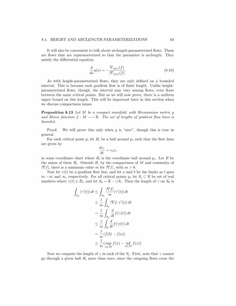
8.4. HEIGHT AND ARCLENGTH PARAMETERIZATIONS 83
It will also be convenient to talk about arclength-parameterized flows. Theseare flows that are reparameterized so that the parameter is arclength. Theysatisfy the differential equation
d
dsη(s) = −
∇η(s)(f)|∇η(s)(f)
. (8.10)
As with height-parameterized flows, they are only defined on a boundedinterval. This is because each gradient flow is of finite length. Unlike height-parameterized flows, though, the interval may vary among flows, even flowsbetween the same critical points. But as we will now prove, there is a uniformupper bound on this length. This will be important later in this section whenwe discuss compactness issues.
Proposition 8.13 Let M be a compact manifold, with Riemannian metric gand Morse function f : M −→ R. The set of lengths of gradient flow lines isbounded.
Proof: We will prove this only when g is “nice”, though this is true ingeneral.
For each critical point pi let Bi be a ball around pi such that the flow linesare given by
dxidt
= cixi
in some coordinate chart where Bi is the coordinate ball around pi. Let B bethe union of these Bi. Outside B, by the compactness of M and continuity of|∇f |, there is a minimum value m for |∇f |, with m > 0.
Now let γ(t) be a gradient flow line, and let a and b be the limits as t goesto −∞ and ∞, respectively. For all critical points pi let Si ⊂ R be set of realnumbers where γ(t) ∈ Bi, and let S0 = R− ∪Si. Then the length of γ on S0 is∫
S0
|γ′(t)| dt ≤∫S0
|∇f |m
|γ′(t)| dt
≤ 1m
∫S0
〈∇f, γ′(t)〉 dt
=1m
∫S0
d
dtf(γ(t)) dt
≤ 1m
∫R
d
dtf(γ(t)) dt
=1m
(f(b)− f(a))
≤ 1m
( supx∈M
f(x)− infx∈M
f(x))
Now we compute the length of γ in each of the Si. First, note that γ cannotgo through a given ball Bi more than once, since the outgoing flows cross the
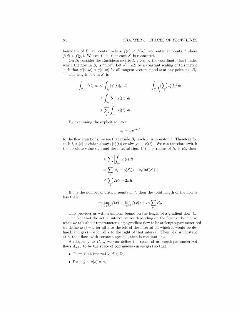
84 CHAPTER 8. SPACES OF FLOW LINES
boundary of Bi at points c where f(c) < f(pi), and enter at points d wheref(d) > f(pi). We see, then, that each Si is connected.
On Bi consider the Euclidean metric E given by the coordinate chart underwhich the flow in Bi is “nice”. Let g′ = kE be a constant scaling of this metricsuch that g′(v, w) > g(v, w) for all tangent vectors v and w at any point x ∈ Bi.
The length of γ in Si is∫Si
|γ′(t)| dt <∫Si
|γ′(t)|g′ dt =∫Si
√∑i
x′i(t)2 dt
≤∫Si
∑i
|x′i(t)| dt
≤∑i
∫Si
|x′i(t)| dt.
By examining the explicit solution
xi = aie−cit
to the flow equations, we see that inside Bi, each xi is monotonic. Therefore foreach i, x′i(t) is either always |x′i(t)| or always −|x′i(t)|. We can therefore switchthe absolute value sign and the integral sign. If the g′ radius of Bi is Ri, then
≤∑i
∣∣∣∣∫Si
x′i(t) dt∣∣∣∣
=∑i
|xi(sup(Si))− xi(inf(Si))|
≤∑i
2Ri = 2nRi
If c is the number of critical points of f , then the total length of the flow isless than
1m
( supx∈M
f(x)− infx∈M
f(x)) + 2n∑pi
Ri.
This provides us with a uniform bound on the length of a gradient flow. The fact that the actual interval varies depending on the flow is irksome, so
when we talk about reparameterizing a gradient flow to be arclength-parameterized,we define η(s) = a for all s to the left of the interval on which it would be de-fined, and η(s) = b for all s to the right of that interval. Then η(s) is constantat a, then flows with constant speed 1, then is constant at b.
Analogously to Ha,b, we can define the space of arclength-parameterizedflows Aa,b,t to be the space of continuous curves η(s) so that
• There is an interval [c, d] ⊂ R,
• For s ≤ c, η(s) = a,

8.5. COMPACTNESS ISSUES CONCERNING MODULI SPACES 85
• For s ≥ d, η(s) = b,
• For s ∈ (c, d), η(s) satisfies (8.10), and
• η(0) ∈W (a, b)t.
Exercise 8.4 Analogously to the proof of Proposition 8.12, prove that Aa,b,t isdiffeomorphic to W (a, b)t.
8.5 Compactness issues concerning moduli spaces
From Example 8.1, we see that some moduli spaces, like M(a, b), are compact,and others, like M(a, d), are not. Consider the situation with M(a, d), which isa union of four open intervals. Take the interval corresponding to the northeastcorner of the figure. As we move along the space of flows to the top, we seem toapproach a union of two flow lines: one from a to b and one from b to d. If wemove instead to the bottom, we appear to approach another union of two flowlines: from a to c then from c to d.
These unions might be called “piecewise flows” or “broken flows” in analogyto phrases like “piecewise continuous” or “piecewise linear”. Of course, theanalogy is not complete since the gradient flow from a to b has as its domainthe entire real line, and if you wanted to tack on the flow from b to d you wouldhave no more domain to use. But if we take arclength parameterization orheight-parameterization this problem disappears.
Along these lines, consider the following (erroneous) view of the convergencewe are observing: let η1, η2, ... be a sequence in M(a, d) that goes upward inthe example we are considering, and for each ηi, let γi be a gradient flow in Fa,brepresenting ηi ∈ Fa,b/R. It is not true that γi converges to a piecewise flow,or indeed, that it converges at all. We can choose γi so that it converges to theflow from a to b; or we can choose it so that it converges to the flow from bto d; or we can choose it so that it converges to the constant flow at b; or theconstant flow at a; or the constant flow at d. We can choose the lift so that itdoes not converges at all.
Exercise 8.5 Convince yourself that all these choices can be made.
The sense that a sequence of flows in the moduli space M(a, d) may convergeto piecewise flows must involve the space M(a, b) directly, without choosing liftsback to Fa,b. This can be done through height-parameterization or arclength-parameterization, and in that context piecewise flows, and the convergence topiecewise flows, are easy to describe.
In this section, we will prove that the only way the moduli spaces can failto be compact is because of the broken flow lines. Later, we will form a com-pactification of the moduli space that includes these broken flow lines, and showthat this compactification is compact, and that the neighborhood of these bro-ken flow lines in the compactification is well-behaved, in the sense that thecompactification is a manifold with corners.

86 CHAPTER 8. SPACES OF FLOW LINES
To state these results, we first need a definition.
Definition 8.14 Suppose that a and b are critical points of f . Then we saythat a > b if W (a, b) is nonempty; equivalently if there is a flow line γ(t) withthe property that
limt→∞
γ(t) = a, limt→−∞
γ(t) = b.
Define l(a, b) to be the largest integer l for which there is a chain of criticalpoints a = a0 > a1 > · · · > al > al+1 = b and we say that b is a successor of aif l(a, b) = 1, i.e. there is no critical point c with a > c > b.
Lemma 8.15 Let αn be a sequence in the moduli space M(a, b) and supposethat αn does not have a convergent subsequence in M(a, b) as n → ∞. Thenthere is a subsequence of αn and a finite sequence of critical points
a = a0 > a1 > · · · > al > al+1 = b
with l ≥ 1 and flow lines γi joining ai−1 to ai, where 1 ≤ i ≤ l, with thefollowing property. Given ε > 0 there is an integer N > 0 such that
d(γi, αn) = inftd(γi(0), αn(t)) < ε
for all n ≥ N and in the subsequence.
Proof: Let t be a fixed value between f(b) and f(a). We view M(a, b) asthe space of arclength-parameterized flows Aa,b,t.
We first show that αn is equicontinuous. If ε > 0, we take δ = ε, and if|s−s0| < δ, then by the Mean Value theorem, |αi(s)−αi(s0)| ≤ max |αi||s−s0| <δ = ε.
Since the manifold is compact, the sequence is uniformly bounded. By theArzela-Ascoli theorem, the sequence has a convergent subsequence, uniformlyon compact sets. By Proposition 8.13, the domain can be taken to be sucha compact set. Without loss of generality, we will assume that our sequenceis such a convergent subsequence. The only question is whether the limit is apiecewise flow.
If αi(s0) converges to a critical point, we will say nothing of regularity. Ifit does not converge to a critical point, we can find an interval [a, b] around s0and a subsequence so that αi(s0) is bounded away from a critical point.
Away from critical points, V (α) = − ∇α(f)|∇α(f)| is a continuous vector field.
As such, if αi(s) converges uniformly on [a, b] to α(s), then we consider theconvergence of V (αi(s)) on [a, b].
Certainly, V (α) is uniformly continuous on the compact subset of M con-taining αi([a, b]) but excluding small balls around the critical points of f . Ifε > 0, we choose the δ involved in uniform continuity of V (α) in the domainjust described. Then by the uniform convergence of αi, we can choose an N sothat |αi(s)− α(s)| < δ for all i > N .

8.5. COMPACTNESS ISSUES CONCERNING MODULI SPACES 87
So|V (αi(s))− V (α(s))| < ε.
In other words, αi(s) = − ∇f|∇f | αi(s) converges uniformly to − ∇f
|∇f | α(s).The fact that αi(s) converges uniformly to α(s) and αi(s) converges uni-
formly implies that limi→∞ αi(s) = α(s). Since αi(s) converged uniformly to− ∇f|∇f | α(s), we have that
α(s) = − ∇f|∇f |
α(s),
in other words, that α(s) is on a flow line except where α(s) is a critical point.Let M be a compact Riemannian manifold without boundary, and f : M →
R a C2 Morse function. Let M(a, b) be the moduli space of Morse flows betweencritical points a and b (with parametrization). Note that by associating eachwith their value at 0, we can associate M(a, b) with the set of points of M whichlie on flows from a to b. Let M(a, b) be the union
M(a, b) =⋃
c1,c2,...,ck
M(a, c1)× · · · ×M(ck, b)
topologized as a subset of M .
Theorem 8.16 The space M(a, b) is compact.
Proof:
[ ... in chap3.8? ]
[ [From chap 5:] ]
One way of viewing this retraction is in terms of the flow energy of a curve
α : (s0, s1) −→M
which is defined to be
Es0s1 (α) =12
∫ s1
s0
(|dαdt
(s)|2 + |∇α(s)(f)|2)ds.
Lemma 8.17
Es0s1 (α) = f(α(s0))− f(α(s1)) +12
∫ s1
s0
(|dαdt
(s) +∇α(s)(f)|2)ds.

88 CHAPTER 8. SPACES OF FLOW LINES
Proof: This lemma follows from integrating the equality∣∣∣∣dαdt (s) +∇α(s)(f)∣∣∣∣2 =
⟨dα
dt(s) +∇α(s)(f),
dα
dt(s) +∇α(s)(f)
⟩=∣∣∣∣dαdt (s)
∣∣∣∣2 +∣∣∇α(s)(f)
∣∣2 + 2⟨dα
dt(s), ∇α(s)(f)
⟩=∣∣∣∣dαdt (s)
∣∣∣∣2 +∣∣∇α(s)(f)
∣∣2 + 2df(dα
dt(s)).
Now let a and b be critical points of f and let Pa,b be the space of L2 -
convergent paths α : R −→M such that
limt→−∞
α(t) = a, limt→+∞
α(t) = b.
L2 convergence means that∫∞−∞ |dαdt (s)|
2ds < ∞. This lemma shows that theabsolute minima of E∞−∞ : Pa,b −→ R are precisely those parameterized pathsin Pa,b which satisfy the flow equations. This is the space we referred to as Fa,b.
[Chap 3.7Attaching map Franks’ theorem ? Maybe later? Case where critical points
are successors? Case where relative dimension is 1Chap 3.8Gluing? Fa,b tubular neighborhood in Pa,b Gluing Behavior of ends Manifold
with cornersChap 3.9Hutchings compactification of Wu(a) examples (including hexagon) Com-
pactness Behavior of ends CW complex explicitly]
8.6 The Morse–Smale chain complex
We have seen that a smooth manifold can be described as a CW complex, witha cell of dimension λ for each critical point of index λ. We also know thatthe homology of a CW complex can be computed from the cells of the CWcomplex by defining a λ-chain to be a formal sum of cells of dimension λ (takenwith orientation), and by defining boundary homomorphisms to describe thegeometric boundary of the cells in question.
We can therefore compute the homology of the manifold using a Morse–Smale function f : Mn −→ R directly, by defining the following complex:
For each integer i with 0 ≤ i ≤ n (where n is the dimension of the manifold),let Ci be the free abelian group generated by critical points of f of index i. Let

8.6. THE MORSE–SMALE CHAIN COMPLEX 89
∂i : Ci −→ Ci−1 be defined on c a critical point of index i as
∂ic =∑b
nc,bb
where the sum is taken over all critical points b of index i − 1, and nc,b ∈ Zis the number of flow lines from c to b, taken with sign. To define ∂i on moregeneral chains (sums of critical points) we extend it linearly.
[ Explain why nc,b is finite (0-dimensional, compact).Explain where the sign comes from (orientation) ]
Proposition 8.18 ∂2 = 0
Proof: [ Need gluing theorem ] Let c be a critical point of f of index i. We
will compute ∂∂c:
∂∂c = ∂∑b
nc,bb
=∑b
nc,b∂b
=∑b
nc,b∑a
nb,aa
=∑a
(∑b
nc,bnb,a
)a
where b ranges over critical points of index i − 1 and a ranges OBover criticalpoints of index i− 2. The sum ∑
b
nc,bnb,a
can be taken over all critical points b of index i− 1 for which there exist flowsfrom c to b and flows from b to a.
By the compactness theorem, M(c, a) is a compact manifold with corners.Since the relative index is two, there can only be corners of codimension one.Therefore, M(c, a) is a manifold with boundary. The boundary is⋃
b
M(c, b)×M(b, a)
which is a set of points whose number is∑b
nc,bnb,a
90 CHAPTER 8. SPACES OF FLOW LINES
so this sum, taken with sign, is zero. [ Explain more with sign ] Therefore,
∂2(c) = 0. For more general chains, we simply apply this linearly.
Definition 8.19 The complex
0 0−→ Cn∂n−→ Cn−1
∂n−1−→ · · · ∂2−→ C1∂1−→ C0
0−→ 0
is called the Morse–Smale complex.

Chapter 9
Compactification of theModuli space of flows
9.1 The Compactification and a Simplicial De-composition of a Torus
Lemma 8.15 describes what happens when one approaches the end of a modulispace of flows M(a, b). Namely, one approaches a sequence of flows (whichwe will refer to as a composite flow γ1, . . . , γm where γi ∈ M(ai−1, ai) wherea = a0, a1, . . . , am−1, am = b is a sequence of critical points. This suggests thefollowing compactification theorem. Recall from chapter 6 the partial orderingon critical points defined by setting a1 > a2 if there exists a flow from a1 toa2, that is if M(a1, a2) is nonempty. A sequence a = a0, . . . , an is ordered ifai > ai+1 for all i. Given such a sequence we let s(a) = a0 and e(a) = an. Wedefine the length of this sequence, l(a), to be n− 1. Finally we define
M(a) = M(a0, a1)× · · · ×M(an−1, an).
Theorem 9.1 A compactification of the moduli space of flows M(a, b) is givenby the following space:
M(a, b) = M(a, b) ∪⋃a
M(a)
where the union is taken over all ordered sequences of critical points a withs(a) = a and e(a) = b.
Theorem 9.2 Let f : M −→ R be a Morse function on a compact manifold asabove, and a, a1, and b be critical points for f with a > a1 > b. Then thereexists an ε > 0 and maps
µ : (0, ε]×M(a, a1)×M(a1, b) −→M(a, b)
91

92CHAPTER 9. COMPACTIFICATION OF THE MODULI SPACE OF FLOWS
which we write as(t, γ1, γ2) −→ γ1 t γ2
that satisfies the following properties:
1. µ is a diffeomorphism onto its image.
2. µ satisfies the following associativity law:
(γ1 s γ2) t γ3 = γ1 s (γ2 t γ3)
for all s, t ≤ ε.
3. This associativity property defines maps
µ : (0, ε]l ×M(a) −→M(a, b)
where (a) is any ordered sequence of critical points of length l with s(a) = aand e(a) = b. These maps are also diffeomorphisms onto their images.
4. Define K(a, b) ⊂M(a, b) to be
K(a, b) = M(a, b)−⋃µ((0, ε)l ×M(a)
)where the union is taken over all ordered sequences (a) of length ≥ 1having s(a) = a and e(a) = b. Then K(a, b) is compact.
5. Define the compactification M(a, b) to be the union along µ
M(a, b) = M(a, b) ∪a
⋃µ
[0, ε]l ×M(a).
Then M(a, b) is homeomorphic to K(a, b).
This theorem says that the ends of the moduli space M(a, b) consist ofspaces of half open cubes parameterized by composable sequences of flow lines.The compact space K(a, b) is formed by removing the associated open cubes.The compactification M(a, b) is formed by formally closing the cubes. It shouldtherefore not be surprising that they are homeomorphic. If γ1 ∈ M(a, a1) andγ2 ∈M(a1, b), then the parameter t ∈ (0, ε] in the flow γ1 tγ2 ∈M(a, b) can beviewed as a measure of how close this flow comes to the critical point a1. Thusthe fact that the pairing µ is a diffeomorphism onto its image allows us to viewthe space K(a, b) as the space of flows that stay at least ε away from all criticalpoints other than a and b (in this undefined measure). On the other hand, thehomeomorphic space M(a, b) can be viewed as formally adjoining composite (or“broken”) flows to M(a, b). From now on we will rescale the metric if necessaryso as to be able to assume ε = 1.

9.2. GLUING FLOW LINES AND THE COMPACTIFICATION THEOREM93
9.2 Gluing Flow Lines and the CompactificationTheorem
In this section we will discuss the gluing of flow lines
µ : (0, ε]×M(a, a1)×M(a1, b) −→M(a, b)
and will outline the proof of the compactification Theorem 9.2. Details are tobe found in [?].
To describe the gluing procedure we first need to pick an ε > 0 with the prop-erty that if x and y are two points inM with d(x, y) = δ < ε, where d(x, y) meansthe geodesic distance, then there is a unique geodesic gx,y : [−δ/2, δ/2] −→M ,parameterized by arclength, joining x to y. Now let a, a1, and b be criticalpoints of f and let γ1 be a flow line joining a to a1, and γ2 a flow line from a1
to b. For t ∈ (0, ε/3] we define the “patched curve”
γ1 ∗t γ2 : R −→M
as follows. Let x be the last point on the curve γ1 whose distance from a1
is t (there may be more than one point on γ1 whose distance from a1 is t).Let y be the first point on the curve γ2 whose distance from a1 is t. Nowlet δ be the geodesic distance between x and y and parameterize γ1 so thatit satisfies the initial condition γ1(−δ/2) = x and parameterize γ2 so that itsatisfies γ2(δ/2) = y. Define γ1 ∗t γ2 to be the following curve:
γ1 ∗t γ2(s) =
γ1(s) if s ≤ −δ/2gx,y(s) if s ∈ [−δ/2, δ/2]γ2(s) if s ≥ δ/2
(9.1)
The following is a picture of the patched curve γ1 ∗t γ2.
We observe the following associativity relation.
Lemma 9.3 Let a, a1, a2, and a3 be critical points of f and let γ1, γ2, and γ3
be flow lines in M(a, a1), M(a1, a2), and M(a2, b) respectively. Then for anyt1, t2 ∈ (0, ε/3] there exists a constant k such that
((γ1 ∗t1 γ2) ∗t2 γ3)(s) = (γ1 ∗t1 (γ2 ∗t2 γ3))(s+ k).

94CHAPTER 9. COMPACTIFICATION OF THE MODULI SPACE OF FLOWS
[Note: Since ∗t does not give us flows, and the inputs to ∗t are assumed tobe flows, is doing it twice defined?]
Exercise 9.1 Prove Lemma 9.3.
We observe that the patched flows γ1 ∗t γ2 are not actually flow lines in thatthey do not satisfy the flow equations for all time. However we will prove thatthey are “approximate ” flows in the sense that they lie very close to the spaceof flow lines Fa,b inside the space Pa,b of all curves from a to b. We will showthat a sufficiently small neighborhood of the space of flows Fa,b actually retractsonto Fa,b (in much the same way as a tubular neighborhood of an embeddedsubmanifold retracts onto the submanifold). The glued flow γ1 t γ2 will be theimage under this retraction of γ1 ∗t γ2.
[ –removed flow energy ]
One way of viewing the idea behind the gluing of flows is to first provethat the patched flow γ1 ∗t γ2 lies in an arbitrarily small neighborhood of Fa,b ∼=W (a, b) in Pa,b so long as t < ε and ε is sufficiently small. One then uses calculusof variations to show that for any curve α ∈ Pa,b that is sufficiently close to Fa,b(i.e. sufficiently close to a global minimum of the energy functional E) there isa unique flow line φα of the energy functional E satisfying
1. φα(0) = α
2. lims→∞ φα(s) = α∞ exists and is an absolute minimum of E. That is,α∞ ∈ Fa,b.
The glued flow line would be defined by
γ1 t γ2 = (γ1 ∗t γ2)∞.
Rather than go through the calculus of variations arguments to show thatthis gluing procedure is well defined and satisfies Theorem 9.2, we will insteaduse a different approach involving linearizing the flow equations. This techniquehas broad generalizations outside the context of Morse functions on compactmanifolds. Indeed it is motivated by work of Taubes [?] in the gluing of “in-stantons” in gauge theory. Gluing of instantons will be discussed later in thesenotes.
To set up this approach, let γ ∈ Pa,b and consider the tangent space TγPa,b.It is easy to see that
TγPa,b = α : R −→ TM such that p α = γ, and limt→±∞
α(t) = 0.
Here p : TM −→ M is the projection of the tangent bundle of the underlyingcompact manifold M . We refer the reader to Milnor’s book [?] for a detaileddescription of the tangent bundle TPa,b.

9.2. GLUING FLOW LINES AND THE COMPACTIFICATION THEOREM95
Now consider the vector field on the path space
S : Pa,b −→ T (Pa,b)
defined by
S(γ) =dγ
dt+∇γf.
Notice that the space of flows Fa,b is precisely the set of zeros of the vectorfield S. Using the underlying metric on M , one has a connection on TPa,b (theassociated Levi–Civita connection) that allows us to differentiate the section Sto obtain a family of operators
DγS : TγPa,b −→ TγPa,b γ ∈ Pa,b.
The precise definition of the operator DS is as the image of the section S ∈C∞(TPa,b) under the covariant derivative D induced by the connection,
C∞(TPa,b) = Ω0(Pa,b;TPa,b)D−−−−→ Ω1(Pa,b;TPa,b).
Here we may interpret the one forms
Ω1(Pa,b;TPa,b) = C∞(T ∗(Pa,b)⊗ TPa,b))= C∞(Hom(TPa,b, TPa,b))
where an element φ ∈ C∞(Hom(TPa,b, TPa,b)) assigns to a curve γ ∈ Pa,b alinear operator φ(γ) : TγPa,b −→ TγPa,b.
The following is little more than a check of the definitions.
Lemma 9.4 The vector field S on Pa,b is transverse to the zero section if andonly if for every flow line γ ∈ Fa,b the operator
DγS : TγPa,b −→ TγPa,b
is surjective.
The operator DS can be described explicitly as follows. Let
Hess(f) : TM −→ TM
be the covariant derivative (with respect to the Levi–Civita connection) of thegradient vector field
∇(f) : M −→ TM.
Given a critical point a ∈M and a basis for TaM , Hessa(f) : TaM −→ TaM isrepresented by the matrix of 2nd order partial derivatives of f . From this pointof view of the Hessian it is easy to see that the operator DS has the form
DγS : TγPa,b −→ TγPa,b
α −→ dα
dt+Hessγ(t)(f) α.

96CHAPTER 9. COMPACTIFICATION OF THE MODULI SPACE OF FLOWS
Now according to Theorem 8.1, the Morse–Smale condition is precisely thatthis operator is surjective. So if f is Morse–Smale, we are assured that theoperator DS is surjective for every pair of critical points a and b. Now sinceFa,b is the space of zeros of the vector field S, the surjectivity of the covariantderivative implies that for any γ ∈ Fa,b,
TγFa,b = Ker(DγS) ⊂ TγPa,b.
One parameter families of operators of the form ddt+At, where At is a self adjoint
linear operator have been studied in great detail by Atiyah, Patodi, and Singerin [?]. When these operators are Fredholm (i.e. have finite dimensional kerneland cokernel) then the index (the difference in the dimension of the kernel andcokernel) is given by the spectral flow of At. That is the number of eigenvaluesof At that “flow” from being negative to positive over time t. That is,
(d
dt+At) = lim
t→−∞At)− lim
t→+∞(At)
where (At) is the dimension of the negative eigenspace of At. In our case thisresult confirms what we already knew for simpler reasons; that
dim(Wa,b) = dim(Fa,b) = dim(TγFa,b)
=d
dt+Hessγ(t)) = ind(a)− ind(b).
Even though in our case we knew the dimension of W (a, b) for easier reasons(transversality), being able to relate the dimension of the zeros of a vector fieldwith the index of its covariant derivative is an important general tool.
The argument then continues and shows, using basically only the implicitfunction theorem, that there exists a small neighborhood, P ηa,b of the space offlows Fa,b in the full path space Pa,b and a retraction map
ρ : P ηa,b −→ Fa,b
so that on the level of derivatives,
Dργ : TγPa,b −→ TγFa,b = Ker(DγS)
is the orthogonal projection onto the kernel of the operator DγS.One then shows that for ε sufficiently small, the image of the patching map
(0, ε]×Fa,c ×Fc,b −→ Pa,b
(t, γ1, γ2) −→ γ1 ∗t γ2
takes values in P ηa,b. If one composes with the projection map ρ : P ηa,b −→ Fa,band divides out by the translation action of the real numbers R, one gets aninduced map
µ : (0, ε]×M(a, c)×M(c, b) −→M(a, b)(t, γ1, γ2) −→ γ1 t γ2

9.2. GLUING FLOW LINES AND THE COMPACTIFICATION THEOREM97
This is the map used to prove Theorem 9.2 in [?]. The associativity lawthat µ is required to satisfy (part (2) of Theorem 9.2) follows from Lemma 9.3and the naturality of the projection map ρ. The compactness properties followeasily from Lemma 8.15 and the fact that µ is a local diffeomorphism. This istechnically the most difficult property to verify. It is done by first observingthat since (0, ε]×M(a, c)×M(c, b) and M(a, b) have the same dimension it issufficient to prove that µ is locally one to one. By the inverse function theorem,to do this it is sufficient to check that its differential is one to one at every point(t, γ1, γ2). But since the patching map
(0, ε]×Fa,c ×Fc,b −→ P ηa,b
(t, γ1, γ2) −→ γ1 ∗t γ2
is clearly one to one, and since the derivative of the projection map ρ : P ηa,b −→Fa,b is the orthogonal projection onto Ker(DS), it is sufficient to show thatfor ε chosen sufficiently small, the image of the derivative of the patching mapis never orthogonal to Ker(DS). This is done by a relatively straightforwardcalculation of the Hessian of f along a patched curve. Details of this argumentwill appear in [?].

98CHAPTER 9. COMPACTIFICATION OF THE MODULI SPACE OF FLOWS
Chapter 10
An explicit CW structureon a manifold
In Chapter 5 we saw that a Morse function f on a compact manifold M can beused to show that M is homotopy equivalent to a CW complex. This is obtainedby examining M t = f−1((−∞, t]) for various values of t. For t sufficiently small,M t is empty, and as we pass critical points, we attach cells (up to homotopyequivalence), and as we move t between critical points, we get a diffeomorphism.
In Chapter 6 we saw how the unstable manifold of each critical point is anopen disk, and if f is Morse–Smale, this partitions M into what appears to bea CW complex. We even saw in Chapter 11 how to extract information aboutthe attaching maps.
It is tempting, therefore, to wonder if this partitioning of M into cells isreally a CW complex decomposition. In this chapter we will see that it is, usinga technique due to Hutchings[?].
10.1 The Hutchings closed cell
The main issue to resolve is that in a CW complex, the cells are closed disks,while the unstable manifold Wu(a) of a critical point a ∈ M is an open disk.To fix this situation, consider the following compactification of Wu(a).
Definition 10.1 If a ∈M is a critical point of f : M −→ R, let Wu(a) be the
following union:⋃c1,...,cr
M(a, c1)× · · · ×M(cr−2, cr−1)×W (cr−1, cr)
with the identifications given by the compactness theorem.
[ I know that should have been more explicit. Later. ]
99

100 CHAPTER 10. AN EXPLICIT CW STRUCTURE ON A MANIFOLD
[ Show it is compact.Show it is a disk.Talk about attaching maps again.Prove it is a CW complex ]

Chapter 11
The Attaching maps
We have shown how a manifold M is homotopy equivalent to a CW complex(Theorem 5.7), using a Morse function f . We have also seen how, using a metric,we can obtain the cells of this CW complex as the unstable manifolds Wu(a) foreach critical point. But a CW complex is determined not only by its cells, butby its attaching maps. In this section we explain how to find these attachingmaps.
Let a be a critical point of M , and let t be a real number t < f(a) withf(a)− t sufficiently small.
Proposition 11.1 There is a diffeomorphism of M that sends M t onto it-self and so that the attached disk Dλ in Theorem 5.6 gets sent to Wu(a) ∩f−1[t, f(a)]. In other words, up to a diffeomorphism of M ,
Dλ = Wu(a) ∩ f−1[t0, t1]. (11.1)
Proof: [ Proof goes here ]
This has the following implication for the CW structure of M . Let M(f)be the CW complex associated to the Morse function f : M −→ R as inTheorem 5.7. Let M(f)(q) denote the q-skeleton. It consists of one cell ofdimension p for every critical point of f having index p ≤ q.
[ don’t use (q) skeleton. Instead, r-skeleton. ]
Recall that the data associated with a CW complex is as follows: a collectionof closed λ-dimensional cells D
λ
i , and for each λ-dimensional cell, an attachingmap φλi : Sλ−1
i −→ ∪k<λDλ
i from its boundary to the λ − 1-skeleton. In thisway, we view a CW complex as growing inductively, by first taking a bunch ofzero-cells, then attaching the one-cells, and so on.
The way we have used a Morse function to show the manifold has the ho-motopy type of a CW complex (Theorem 5.7) is similar: we examine M t =
101

102 CHAPTER 11. THE ATTACHING MAPS
f−1((−∞, t]) for various increasing values of t. we start with a zero-cell when tis the minimum value of f . As we increase t, if we do not pass through a criticalvalue, the homotopy type of M t is unchanged; but if we increase it through acritical value, we attach a cell whose dimension is the index of the critical point.Thus, inductively, we attach cells to whatever we have already built.
From the perspective of using unstable manifolds for cells, we might hope toreplace the notion of increasing t with the notion of adding unstable manifoldsdirectly, in the order of increasing values for f . Now, it may be disconcertingthat the order that we are attaching cells is by value for f instead of dimension(as would be the case with CW complexes). But this is irrelevant, since ifind(a) ≥ ind(b), and (f, g) is Morse–Smale, then there are no flows from b toa, and in particular, the unstable manifold from b does not approach cells ofhigher dimension.
[ There might be a need to cite compactness theorems from chap 3.8 ]
11.1 Consecutive critical points: Franks’ theo-rem
Suppose a and b are consecutive critical points, in the sense that there are flowsfrom a to b but no other intermediate flows. That is, there does not exist acritical point c so that there are flows from a to c and flows from c to b.
Let the index of a be p and let r < p be the index of b. Let Dpa ⊂ M(f)(p)
be the associated attaching disk to the critical point a. It is attached by a map
φa : Sp−1a −→M(f)(p−1).
The following is an immediate corollary of (11.1):
Corollary 11.2 The attaching map φa : Sp−1a −→ M(f)(p−1) factors through
the r-skeleton:φa : Sp−1
a −→M(f)(r).
Notice that the quotient of the skeleta is a wedge of r-dimensional spheresindexed by the critical points of index r:
M(f)(r)/M(f)(r−1) '∨
β∈Critr
Srβ
where Critr denotes the set of critical points of index r. Given such a criticalpoint b ∈ Critr we consider the relative attaching map
φa,b : Sp−1 φa−→M(f)(r)p−→M(f)(r)/M(f)(r−1) '
∨β∈Critr
Srβπb−→ Srb (11.2)
where p and πb are the obvious projection maps. We will consider the maps φa,bas elements in the homotopy group πp−1(Sr). As in chapter 2 we can stabilize

11.1. CONSECUTIVE CRITICAL POINTS: FRANKS’ THEOREM 103
to get an element to get an element in the stable homotopy groups of sphereswhich, by abuse of notation we call by the same name
φa,b ∈ πsp−r−1.
By Theorem 2.1 (The Thom–Pontrjagin theorem) we can identify this groupwith the framed cobordism group ηp−r−1. In [?] J. Franks showed how φa,b isrepresented by M(a, b), the moduli space of flow lines between the two criticalpoints a and b, as a framed moduli space.1
Notice that Lemma 8.15 says that M(a, b) is a compact manifold if andonly if b is a successor of a. Notice that in the context of studying the relativeattaching maps (as in equation (11.2)) we are assuming that this is indeed thecase. So M(a, b) is a closed, p − r − 1 dimensional manifold. M(a, b) can begiven a framing as follows. Let t be any regular value between f(a) and f(b).By (11.1) the intersection
Wu(a) ∩ f−1(t)
is a sphere of dimension p− 1 which we denote by Su(a). Similarly, we define
Ss(b) = W s(b) ∩ f−1(t)
which is a sphere of dimension n− p− 1.By construction we have
M(a, b) ∼= W (a, b)t = W (a, b) ∩ f−1(t)
= W s(b) ∩Wu(a) ∩ f−1(t) = W s(b) ∩ Su(a).
Thus we have a natural embedding M(a, b) → Su(a) which has codimension r.The normal bundle of this embedding is the pull-back of the normal bundle ofthe embedding
W s(b) →M
which comes equipped with a unique framing because W s(b), being diffeomor-phic to the disk Dn−r is contractible. This induces a framing α on the normalbundle of M(a, b) → Su(a). Hence the pair (M(a, b), α) determine an elementin the framed cobordism group
(M(a, b), α) ∈ ηp−r−1
Theorem 11.3 (Frank’s theorem [?]) Under the Thom–Pontrjagin construc-tion, the relative attaching map
φa,b ∈ πsp−r−1
1Note that this is not a complete description of the attaching map: only the “component”that corresponds to the piece that wraps around the unstable manifold for the one criticalpoint b. Even if we took all these data for each critical point, we still do not have the attachingmap becaues πi(X ∨ Y ) is not necessarily isomorphic to πi(X)× πi(Y ). Furthermore, we areignoring the data that describes how the attaching map maps to the s-skeleton where s < r.But we can have some fun at the r stage, and so we will.

104 CHAPTER 11. THE ATTACHING MAPS
corresponds to the framed moduli space of flows
(M(a, b), α) ∈ ηp−r−1.
Proof: By (11.1) the source sphere in the attaching map
φa,b : Sp−1 −→ Sr,
being the boundary of the disk represented by the critical point a, is Su(a).Furthermore, the composition given in (11.2) defining φa,b is homotopic to thecomposition (which by abuse of notation we also call φa,b,
φa,b : Su(a)φa−−−−→ M(f)(r)
proj−−−−→ M(f)(r)/(M(f)(r) −W s(b)) = Sr.
The transversality condition (i.e. the Morse–Smale condition) implies that thebase point ∗ ∈ Sr is a regular value of φa,b. Furthermore the inverse image
φ−1a,b(∗) = Su(a) ∩ Ss(b) = M(a, b).
The induced framing on M(a, b) from the framing of ∗ ∈ Sr is clearly theframing α described above. Hence (M(a, b), α) is the image of φa,b under theThom–Pontrjagin construction.
11.2 Relative index one
Now suppose a and b are critical points of relative index one. Say (a) = pand (b) = p − 1. Then the space of flows, (M(a, b), α) is a zero dimensional,framed, compact manifold; that is a finite set of points (flow lines) with signsattached to them induced by the framing. This is what we normally call an“orientation”. And indeed, an orientation is precisely what we need on a CWcomplex to define homology.
Let n(a, b) ∈ Z denote the signed number of flow lines:
n(a, b) =∑
γ∈M(a,b)
α(γ)
where α(γ) = ±1 is the sign associated to the flow line γ by the framing α.
n(a, b) ∈ Z = η0 = πs0
is therefore the integer given by the degree of the relative attaching map
φa,b : Sp−1 −→ Sp−1.
This allows us to compute the boundary homomorphism in the Morse–Smalecomplex (5.1). Recall that in this complex, Cp is the free abelian group gener-ated by Critp. Let [a] ∈ Cp denote the generator corresponding to the criticalpoint a.

11.2. RELATIVE INDEX ONE 105
Corollary 11.4 The coefficient of [b] ∈ Cp−1 of the boundary ∂p[a], 〈∂p[a], [b]〉,is given by the formula
〈∂p[a], [b]〉 = n(a, b) ∈ Z.
We note that this formula for the Morse–Smale complex is implicit in thework of Smale (see [?]). As described above it should be viewed as a specialcase of the attaching map formulae of Franks [?]. However the formulae incorollary 11.4 seems to have first been explicitly given in the literature by Witten[?].

106 CHAPTER 11. THE ATTACHING MAPS

Part III
Category of gradient flows
107


Chapter 12
The Flow Category of aMorse Function
Let f : M −→ R be a Morse function on a compact manifold. In this chapterwe will construct a topological category Cf whose objects are the critical pointsof f and where the space of morphisms between two critical points a and b isa compactification, M(a, b) of the moduli space of flows M(a, b). We will thenprove that the classifying space BCf is homeomorphic to the manifold M . Thiswill give M the structure of an explicit simplicial space (i.e. the nerve of Cf )and will complete our goal of recovering the topology of the manifold directlyand explicitly in terms of the space of flows of the gradient vector field.
[ Removed: Compactification argument, now in Chap 3.8 ]
We will state this compactification theorem more precisely later, and inparticular describe the topology of M(a, b). Then the theorem will be provedin the next section. In this section we will describe how it will be used to definethe category induced by a Morse function and state how its classifying space isrelated to the underlying manifold. We will then consider the examples of twodimensional tori. We will begin by stating the main theorem to be discussed inthis chapter. The details of the proof of this theorem will appear in [?].
Theorem 12.1 Let f : M −→ R be a Morse function on a compact manifoldsatisfying the Morse–Smale transversality conditions. Consider the topologicalcategory Cf whose objects are the critical points of f , and whose spaces of mor-phisms are the compactified moduli spaces,
Mor(a, b) = M(a, b).
Composition in this category is given by the inclusion
M(a, b)×M(b, c) →M(a, c)
109

110 CHAPTER 12. THE FLOW CATEGORY OF A MORSE FUNCTION
described in the compactification Theorem 9.1. Then there is a natural homeo-morphism of the classifying space of this category with the underlying manifold
BCf∼=−−−−→ M.
Notice that this theorem defines an explicit simplicial space description (asthe nerve of the category N (Cf )) of the manifold M in terms of the modulispaces of flow lines of the gradient vector field of the Morse function f . Indeedthe k-simplices of this decomposition are parameterized by the space of k-tuplesof “composable” flow lines. We will discuss implications of this theorem infollowing chapters. The main goal of this section is to illustrate this simplicialdecomposition for a particular example of a Morse–Smale flow on a torus. Inorder to do this we need a more precise version of the compactification theorem.This theorem will give a detailed description of the ends of moduli spaces.
12.1 Torus example
The homeomorphism between K(a, b) and M(a, b) allows us to define the cat-egory Cf in two equivalent (isomorphic) ways. The first way, as described inTheorem 12.1, is to let the space of morphisms between critical points a and bbe M(a, b), where the composition law is given by
M(a, b)×M(b, c) −→M(a, c)(γ1, γ2) −→ γ1 0 γ2.
The other equivalent definition is to let the space of morphisms betweencritical points a and b be K(a, b), where the composition law is given by
K(a, b)×K(b, c) −→ K(a, c)(γ1, γ2) −→ γ1 ε γ2.
For the purposes of the following diagrams we will use the second way of definingCf .
Consider the following figure depicting a Morse–Smale flow on the torus.
Here we view the two-torus as embedded in ordinary three-space, standing

12.1. TORUS EXAMPLE 111
on one of its ends with the hole facing the reader, but tilted slightly toward thereader. We let f be the height function.
There are four critical points; a has index 2, b and c have index 1, and d hasindex 0. As the figure depicts, the moduli spaces M(a, b), M(a, c), M(b, d), andM(c, d) are all spaces consisting of two distinct points each. We will denote theseflows by αi, βi, γi, and δi respectively. All points on the torus not lying on anyof these flows is on a flow in M(a, d). This moduli space is one dimensional, andindeed is the disjoint union of four open intervals. Thus K(a, d) is the disjointunion of four closed intervals. If the torus is viewed in the usual way as a squarewith opposite sides identified, then these flows can be depicted as follows.
Now consider the simplicial description in the classifying space BCf . Thevertices correspond to the objects of the category Cf , that is the critical points.Thus there are four vertices. There is one one simplex (interval) for each mor-phism (flow line), glued to the vertices corresponding to the starting and end-points of the flows. Notice that the points in K(a, d) index a one parameterfamily of one simplices attached to the vertices labelled by a and d. Finallyobserve that there is a two-simplex for every pair of composable flows. Thereare eight such pairs (coming from the four points in each of the product mod-uli spaces M(a, b) ×M(b, d) and M(a, c) ×M(c, d).) A two-simplex labelledby a pair of flows, say (α, β) will have its three faces identified with the onesimplices labelled by α, β, and α1 β respectively. Notice that all higher dimen-sional simplices in the nerve N (Cf ) are degenerate and so do not contribute tothe geometric realization. The following figure depicts the resulting simplicialstructure of the classifying space and illustrates Theorem 12.1 that this space

112 CHAPTER 12. THE FLOW CATEGORY OF A MORSE FUNCTION
is homeomorphic to the underlying manifold.
12.2 Proof of Theorem 12.1
In this section we give a proof of the main theorem of this chapter, Theorem 12.1.That is, we identify the manifoldM with the classifying space of the category Cf .Recall that this theorem proposes to describe M as a simplicial space, wherethe simplices are parameterized by cartesian products of the moduli spaces,M(a, b), or equivalently, K(a, b). We begin by describing a filtration of thespaces M(a, b).
By scaling the metric of M if necessary, we can assume that the constantε in the statement of Theorem 9.2 is 1 and so we will now drop this from thenotation. We can think of the set K(a, b) of Theorem 9.2 as the space of flowlines from a to b which keep distance of at least 1 from any critical points cwith a > c > b. More generally we can filter the space M(a, b) by saying that acurve in M(a, b) has filtration k if it gets within distance less than 1 of at mostk intermediate critical points. Precisely, we define
K(k)(a, b) =⋃l≤k
⋃a>a1>···>al>b
µ([0, 1]l ×K(a, a1)× . . .K(al, b)
).
so that K(0)(a, b) = K(a, b) and
K(k−1)(a, b) ⊆ K(k)(a, b).
Thus γ is in K(k)(a, b) if and only if γ can be decomposed as
γ = γ0 s1 · · · slγl
where γi ∈ K(ai−1, ai), 0 ≤ si ≤ 1 for all i, and l ≤ k.
Lemma 12.2
K(k)(a, b) \ K(k−1)(a, b) ∼=⊔
a>a1>···>ak>b
[0, 1)k ×K(a, a1)× . . .K(ak, b)

12.2. PROOF OF THEOREM 12.1 113
Proof: This is obvious, I hope.
Lemma 12.3 ⋃K(k)(a, b) = M(a, b)
Proof: This too is obvious, I hope. Let a = (a0, . . . , al+1) denote an arbitrary decreasing sequence of critical
points with length l(a) = l, starting point s(a) = a0 = a and ending pointe(a) = al+1 = b. We define
K(a) = K(a0, a1)× · · · × K(al, al+1).
Using these lemmas we see that the map⊔l
⊔l(a)=l
[0, 1]l ×K(a) −→M(a, b)
defined by(s1, . . . , sl; γ0, . . . , γl) −→ γ0 s1 · · · sl
γl
is onto and therefore M(a, b) can be recovered by imposing an equivalence rela-tion on the above disjoint union. It is straightforward to extract this equivalencerelation; it is generated by
(s1, . . . , si−1, 1, si+1, . . . , sl; γ1, . . . , γl) '(s1, . . . , si−1, si+1, . . . , sl; γ1, . . . , γi−1 1 γi, . . . , γl).
Thus the relations only involve the faces of the cubes which do not contain thepoint (0, . . . , 0).
From this argument we draw the following conclusion.
Theorem 12.4M(a, b) =
⊔l
⊔l(a)=l
[0, 1]l ×K(a)/ '
The next step is to go from this description of the spaces M(a, b) to one ofthe manifold M . Let γ ∈M(a, b) be a flow line. Then we may compactify γ byadding the points a and b to form the curve γ. This curve is closed in the sensethat it contains all of its limit points. The function f is decreasing along flowlines and so it gives a natural diffeomorphism
f : γ −→ [f(b), f(a)].
Now suppose that γ = γ00 · · ·0γl is a point of M(a, b) which is not in M(a, b).Thus γ0, . . . , γl is a sequence of flow lines joining critical points a > a1 > · · · >al > b. In this case define
γ = γ0 ∪ · · · ∪ γl,

114 CHAPTER 12. THE FLOW CATEGORY OF A MORSE FUNCTION
so γ is a curve in M joining a to b; in an obvious sense γ is a piecewise flow linejoining a to b. The function f defines a diffeomorphism
f : γi −→ [f(ai), f(ai−1)]
and these diffeomorphisms piece together to define a homeomorphism
f : γ −→ [f(b), f(a)].
This shows that each element in M(a, b) can be identified with a well definedcurve γ : [f(b), f(a)] −→ M parameterized by the inverse of the above home-omorphism. However, with this parameterization, none of these curves satisfythe flow equations. In any case we get a map
φ : [f(b), f(a)]×M(a, b) −→M
whose image is the closure of the space W (a, b) ⊂ M since we have added toW (a, b) all points on the curves γ : [f(b), f(a)] −→ M where γ ∈ M(a, b).Therefore the map⊔
a
[f(al+1), f(a0)]× [0, 1]l ×K(a) −→M
defined by(t; s1, . . . , sl; γ0, . . . , γl) −→ (γ0 s1 · · · sl
γl)(t)
is onto. The disjoint union is taken over all decreasing sequences of criticalpoints a = (a0, . . . , al+1). Once more it is not difficult to extract the appropriateequivalence relation on the disjoint union. Given a sequence a of critical pointsas above with l(a) = l, we define
Ja = [f(al+1), f(a0)], I l(a) = [0, 1]l.
Now we define
Definition 12.5Rf =
⊔a
Ja × I l(a) ×K(a)/ ∼
where the relations ∼ are given by
(t; s1, . . . , si−1, 0, si+1, . . . , sl; γ0, . . . , γl) ∼(t; s1, . . . , si−1; γ0, . . . , γi−1), if t ∈ [f(ai), f(a0)](t; si+1, . . . , sl; γi+1, . . . , γl), if t ∈ [f(al+1), f(ai)]
(12.1)
and
(t; s1, . . . , si−1, 1, si+1, . . . , sl; γ0, . . . , γl) ∼(t; s1, . . . , si−1, si+1, . . . , sl; γ0, . . . , γi−1 1 γi, . . . , γl) (12.2)
The map φ respects the equivalence relation ∼ so gives a well defined map
Rf −→M.

12.2. PROOF OF THEOREM 12.1 115
Theorem 12.6 The mapφ : Rf −→M
is a homeomorphism.
Proof: The first step is to check that the second set of relations are theonly relations which can occur if all the si’s are non-zero. This follows from thefact that if two flow lines have a point in common then they are equal togetherwith the previous theorem. If one of the si’s is zero then we are dealing with apiecewise flow line. If two piecewise flow lines have a point in common then thispoint must be one of the joining points or else they have a common segment.An elementary analysis leads to the conclusion that the only identificationswhich can take place if one of the si’s is zero are consequences of the first set ofrelations.
Since the spaces K(ai−1, ai) are diffeomorphic to the compactified spacesM(ai−1, ai) in such a way that the composition in the category corresponds to1, this shows us how to recover the manifold M from the category Cf . To proveTheorem 12.1 we are therefore reduced to the combinatorial exercise necessaryto identify the space Rf with the classifying space BCf . Recall from chapter 13the definition of the classifying space of the category Cf . Comparing it withDefinition 12.5 of the space Rf we see that these spaces are very similar butthey are not obviously the same. The essential difference is that Rf is built upout of cubes whereas the classifying space is built out of simplices. Nonethelessthese two spaces are homeomorphic.
Theorem 12.7 There is a homeomorphism
Rf∼= BCf .
Proof: The main point of this argument is that the equivalence relationsused to build Rf can be imposed in two steps; the first step turns the cubesinto simplices and the second step then imposes the gluing relations among thesimplices that make up BCf . To see this precisely we first look at the image ofa single cube
Ja × I l = Ja × I l × (γ0, . . . , γl)
in the quotient space Rf . Define
ai = (a0, . . . ai−1, ai+1, . . . al+1) where 0 ≤ i ≤ l + 1
and mapsδi : Jai
× I l−1 −→ Ja × I l
by the formulas
δi(t; s1, . . . , sl−1) =
(t; 0, s1, . . . , sl−1), if i = 0(t; s1, . . . , si−1, 1, si, . . . , sl−1), for 1 ≤ i ≤ l
(t; s1, . . . , sl−1, 0), if i = l + 1.

116 CHAPTER 12. THE FLOW CATEGORY OF A MORSE FUNCTION
Now consider the spacesJa × I l−1/ ∼
where we make the following list of identifications: If 1 ≤ i ≤ l so that Ja = Jai
then
(t; s1, . . . si−1, 0, si+1, . . . , sl)
∼
(t; s1, . . . , si−1, 0, s′i+1, . . . s
′l) if f ∈ [f(ai), f(a0)]
(t; s′1, . . . , s′i−1, 0, si+1, . . . , sl), if t ∈ [f(al+1, f(ai)];
and in the case i = 0, 1 then
(t; 0, s2, . . . , sl) ∼ (t; 0, s′2, . . . s′l) if t ∈ [f(a1), f(a0)]
(t; s1, . . . , sl−1, 0) ∼ (t; s′1, . . . , s′l−1, 0) if t ∈ [f(al+1, al)];
finally
(f(al+1); s1, . . . , sl) ∼ (f(al+1); s′1, . . . , s′l)
(f(a0); s1, . . . , sl) ∼ (f(a0); s′1, . . . , s′l).
Note that if two points in Ja×I l are identified then they have the same imageinRf , so we can equally well build the spaceRf from the spaces Ja×I l/ ∼. Themain point is the space Ja×I l/ ∼ is naturally homeomorphic to a l+1-simplex,with the δi map corresponding to the inclusions of the ith face. That is, we havethe following combinatorial result, whose verification is straightforward.
Lemma 12.8 There are homeomorphisms
ha : Ja × I l/ ∼−→ ∆l+1
which make the following diagrams commute
Ja × I l/ ∼ ha−−−−→ ∆l+1
δi
x xδi
Jai× I l−1/ ∼ −−−−→
hai
∆l
where the left hand δi the map just constructed, and the right hand δi is theinclusion of the ith face as described in chapter 13.
At this stage we have used up the first relations (12.1). Now we impose therelations (12.2) to get the following result.
Proposition 12.9 There is a homeomorphism
Rf∼=⊔a
∆l(a)+1 ×K(a)/ ∼

12.2. PROOF OF THEOREM 12.1 117
where
(s0, . . . , si−1, 0, si+1, . . . , sl; γ0, . . . , γl) ∼(s1, . . . sl; γ1, . . . , γl) if i = 0(s0, . . . , si−1, si+1, . . . , sl; γ0, . . . , γi−1 1 γi, . . . γl) if 1 ≤ i ≤ l − 1(s0, . . . , sl−1; γ0, . . . , γl−1) if i = l
Proof: This follows from the previous lemma by imposing the second listof relations (12.2).
Notice that Theorem 12.7 now follows from this theorem by the definition ofthe classifying space of the category Cf . As noted before, Theorem 12.7 impliesTheorem 12.1.

118 CHAPTER 12. THE FLOW CATEGORY OF A MORSE FUNCTION

Chapter 13
Simplicial Sets andClassifying Spaces
[ Add more picturesIn the last chapter we saw how the topology of the framed moduli spaces
of gradient flows of a Morse function determine the relative attaching maps ina CW complex homotopy equivalent to the manifold. In the next chapter wewill strengthen this to show how these moduli spaces determine a simplicialstructure of the manifold itself. That is, the topology of the moduli spacesdetermine the full topology of the manifold as a simplicial space; not only thehomotopy type. In order to describe how this works we need the language ofsimplicial sets and spaces as well as the notion of a simplicial classifying space.We discuss these notions in this chapter. Good references for this theory are[?][?][?].
13.1 Simplicial Sets and Spaces
The idea of simplicial sets is to provide a combinatorial technique to study cellcomplexes built out of simplices; i.e. simplicial complexes. A simplicial complexX is built out of a union of simplices, glued together along faces. Thus if Xn
denotes the indexing set for the n-dimensional simplices of X, then we can write
X =
⋃n≥0
∆n ×Xn
/ ∼
where ∆n is the standard n-simplex in Rn;
∆n = (t1, . . . , tn) ∈ Rn | 0 ≤ tj ≤ 1, andn∑i=1
ti ≤ 1.
119
120 CHAPTER 13. SIMPLICIAL SETS AND CLASSIFYING SPACES
The gluing relation in this union can be encoded by set maps among the Xn’sthat would tell us for example how to identify an n − l-simplex indexed by anelement of Xn−1 with a particular face of an n-simplex indexed by an elementof Xn. In particular, for every x ∈ Xn, we have n + 1 “faces” ∂0, . . . , ∂n inXn−1, and we have n + 1 “degenerate simplices” σ0, . . . , σn in Xn+1 that aren+ 1-simplices that are “degenerate” in the sense that they are projected ontoone of their faces (geometrically, these will all appear to be the same as x;but the parameterization of them as simplices is n + 1-dimensional instead ofn-dimensional, and one of the directions is degenerate).
Thus in principle, simplicial complexes can be studied purely combinatoriallyin terms of the sets Xn and set maps between them. The notion of a simplicialset makes this idea precise.
Definition 13.1 A simplicial set X∗ is a collection of sets
Xn, n ≥ 0
together with set maps
∂i : Xn −→ Xn−1 and sj : Xn −→ Xn+1
for 0 ≤ i, j ≤ n called face and degeneracy maps respectively. These maps arerequired to satisfy the following compatibility conditions
∂i∂j = ∂j−1∂i for i < j
sisj = sj+1si for i < j
and
∂isj =
sj−1∂i for i < j
1 for i = j, j + 1sj∂i−1 for i > j + 1
As mentioned above, the maps ∂i and sj encode the combinatorial infor-mation necessary for gluing the simplices together. To say precisely how thisworks, consider the following maps between the standard simplices:
δi : ∆n−1 −→ ∆n and σj : ∆n+1 −→ ∆n
for 0 ≤ i, j ≤ n defined by the formulae
δi(t1, . . . , tn−1) =
(t1, . . . , ti−1, 0, ti, . . . , tn−1) for i ≥ 1(1−
∑n−1q=1 tq, t1, . . . , tn−1) for i = 0
and
σj(t1, . . . , tn+1) =
(t1, . . . , ti−1, ti + ti+1, ti+2, . . . , tn+1) for i ≥ 1(t2, . . . , tn+1) for i = 0 .

13.1. SIMPLICIAL SETS AND SPACES 121
δi includes ∆n−1 in ∆n as the ith face, and σj projects, in a linear fashion, ∆n+1
onto its jth face.We can now define the space associated to the simplicial set X∗ as follows.
Definition 13.2 The geometric realization of a simplicial set X∗ is the space
‖X∗‖ =
⋃n≥0
∆n ×Xn
/ ∼
where if t ∈ ∆n−1 and x ∈ Xn, then
(t, ∂i(x)) ∼ (δi(t), x)
and if t ∈ ∆n+1 and x ∈ Xn then
(t, sj(x)) ∼ (σj(t), x).
In the topology of ‖X∗‖, each Xn is assumed to have the discrete topology, sothat ∆n ×Xn is a discrete set of n-simplices.
Thus ‖X∗‖ has one n-simplex for every element of Xn, glued together in away determined by the face and degeneracy maps.
Example 13.1 Consider the simplicial set S∗ defined as follows. The set ofn-simplices is given by
Sn = Z/(n+ 1)Z, generated by an element τn.
The face maps are given by
∂i(τ rn) =
τ rn−1 if r ≤ i ≤ n
τ r−1n−1 if 0 ≤ i ≤ r − 1.
The degeneracies are given by
si(τ rn) =
τ rn+1 if r ≤ i ≤ n
τ r+1n+1 if 0 ≤ i ≤ r − 1.
Notice that there is one zero simplex, two one simplices, one of them the imageof the degeneracy s0 : S0 −→ S1, and the other nondegenerate (i.e. not inthe image of a degeneracy map). Notice also that all simplices in dimensionslarger than one are in the image of a degeneracy map. Hence we have that thegeometric realization
‖S∗‖ = ∆1/(0 ∼ 1) = S1.

122 CHAPTER 13. SIMPLICIAL SETS AND CLASSIFYING SPACES
Let X∗ be any simplicial set. There is a particularly nice and explicit wayfor computing the homology of the geometric realization, H∗(‖X∗‖).
Consider the following chain complex. Define Cn(X∗) to be the free abeliangroup generated by the set of n-simplices Xn. Define the homomorphism
dn : Cn(X∗) −→ Cn−1(X∗)
by the formula
dn([x]) =n∑i=0
(−1)i∂i([x])
where x ∈ Xn.
Proposition 13.3 The homology of the geometric realization H∗(‖X∗‖) is thehomology of the chain complex
−→ . . .dn+1−−−−→ Cn(X∗)
dn−−−−→ Cn−1(X∗)dn−1−−−−→ . . .
d0−−−−→ C0(X∗).
Proof: It is straightforward to check that the geometric realization ‖X∗‖ isa CW complex and that this is the associated cellular chain complex.
Besides being useful computationally, the following result establishes the factthat all CW complexes can be studied simplicially:
Theorem 13.4 Every CW complex has the homotopy type of the geometricrealization of a simplicial set.
Proof: Let X be a CW complex. Define the singular simplicial set of X ,S(X)∗ as follows. The n-simplices S(X)n is the set of singular n-simplices,
S(X)n = c : ∆n −→ X.
The face and degeneracy maps are defined by
∂i(c) = c δi : ∆n−1 −→ ∆n −→ X
andsj(c) = c σi : ∆n+1 −→ ∆n −→ X.
Notice that the associated chain complex to S(X)∗ as in Proposition 13.3 isthe singular chain complex of the space X. Hence by Proposition 13.3 we havethat
H∗(‖S(X)‖) ∼= H∗(X).
This isomorphism is actually realized by a map of spaces
E : ‖S(X)∗‖ −→ X
13.2. CATEGORIES AND CLASSIFYING SPACES 123
defined by the natural evaluation maps
∆n × S(X)n −→ X
given by(t, c) −→ c(t).
It is straightforward to check that the map E does induce an isomorphism inhomology. In fact it induces an isomorphism in homotopy groups. We will notprove this here; it is more technical and we refer the reader to [?] for details.Note that in the case where X is simply-connected, this would follow from thehomological isomorphism by the Hurewicz theorem. A map between spaces thatinduces an isomorphism in homotopy groups is called a weak homotopy equiva-lence. Thus any space is weakly homotopy equivalent to a CW complex (i.e. thegeometric realization of its singular simplicial set). But by the Whitehead the-orem, two CW complexes that are weakly homotopy equivalent are homotopyequivalent. Hence X and ‖S(X)∗‖ are homotopy equivalent.
We end this section by observing that the notion of simplicial set can begeneralized as follows. We say that X∗ is a simplicial space¡ if it is a simplicialset (i.e. it satisfies Definition 13.1) where the sets Xn are topological spaces andthe face and degeneracy maps
∂i : Xn −→ Xn−1 and sj : Xn −→ Xn+1
are continuous maps. The definition of the geometric realization of a simplicialspace X∗, ‖X∗‖, is the same as in Definition 13.2 with the proviso that thetopology of each ∆n×Xn is the product topology. Notice that since the “set ofn-simplices” Xn is actually a space, it is not necessarily true that ‖X∗‖ is a CWcomplex, and in particular Proposition 13.3 does not hold. However if in facteach Xn is a CW complex and the face and degeneracy maps are cellular, then‖X∗‖ does have a natural CW structure induced by the product CW structureson ∆n ×Xn.
Notice that this simplicial notion generalizes even further. For example asimplicial group would be defined similarly, where each Xn would be a groupand the face and degeneracy maps are group homomorphisms. Simplicial vectorspaces, modules, etc. are defined similarly. The categorical nature of thesedefinitions should by now be coming clear. Indeed most generally one candefine a simplicial object in a category C using definition 13.1 where now theXn’s are assumed to be objects in the category and the face and degeneraciesare assumed to be morphisms. If the category C is a subcategory of the categoryof sets then geometric realizations can be defined as in Definition 13.2. Noticefor example that the geometric realization of a simplicial (abelian) group is atopological (abelian) group.
13.2 Categories and Classifying Spaces
We will now use simplicial techniques to construct classifying spaces of groupsand of categories.

124 CHAPTER 13. SIMPLICIAL SETS AND CLASSIFYING SPACES
Let G be a topological group, and suppose that EG is a contractible spacewith a free, right G action
EG×G −→ EG.
Let BG be the orbit space BG = EG/G. The following are standard facts fromalgebraic topology (bundle theory).
Theorem 13.5 The quotient map EG −→ BG is a principal G-bundle satis-fying the following properties.
1. The homotopy type of BG is well defined. That is, it is independent ofthe choice of EG (so long as EG is contractible with a free G action.)
2. πq(BG) ∼= πq−1(G) so in particular if G is discrete BG is an Eilenberg–MacLane space K(G, 1).
3. (Steenrod’s classification theorem) Let X be any CW complex with a base-point. Give BG a basepoint, and let [X,BG] denote the (based) homotopyclasses of basepoint preserving maps from X to BG. Then there is a bi-jective correspondence
[X,BG]∼=−−−−→ψ
PrinG(X)
where PrinG(X) is the set of isomorphism classes of principal G-bundlesover X. The correspondence ψ is given by
ψ([f ]) = f∗(EG).
Because of this theorem the bundle EG −→ BG is uniquely determined upto homotopy and is referred to as the universal principal G bundle.
We now describe a simplicial space model for the universal principal G -bundle EG −→ BG. Let G be a topological group and let EG∗ be the simplicialspace defined as follows. The space of n-simplices is given by the n + 1-foldcartesian product
EGn = Gn+1.
The face maps ∂i : Gn+1 −→ Gn are given by the formula
∂i(g0, . . . , gn) = (g0, . . . , gi, . . . , gn).
The degeneracy maps sj : Gn+1 −→ Gn+2 are given by the formula
sj(g0, . . . , gn) = (g0, . . . , gj , gj , . . . , gn).
Exercise 13.1 Show that the geometric realization ‖EG∗‖ is contractible. Hint:Let ‖EG∗‖(n) be the n-skeleton,
‖EG∗‖(n) =n⋃p=0
∆p ×Gp+1.

13.2. CATEGORIES AND CLASSIFYING SPACES 125
Then show that the inclusion of one skeleton in the next ‖EG∗‖(n) → ‖EG∗‖(n+1)
is canonically null-homotopic. One way of doing this is to establish a homeo-morphism between ‖EG∗‖(n) and n-fold join G ∗ · · · ∗G. See [?] for details.
Notice that the group G acts freely on the right of ‖EG∗‖ by the rule
‖EG∗‖ ×G =
⋃p≥0
∆p ×Gp+1
×G −→ ‖EG∗‖
(t; (g0, . . . , gp))× g −→ (t; (g0g, . . . , gpg)) .
Thus we can define EG = ‖EG∗‖. The orbit space BG = EG/G has asimilar simplicial structure defined as follows.
Let BG∗ be the simplicial space whose n-simplices are the cartesian product
BGn = Gn. (13.1)
The face and degeneracy maps are given by
∂i(g1, . . . , gn) =
(g2, . . . , gn) for i = 0(g1, . . . , gigi+1, . . . gn) for 1 ≤ i ≤ n− 1(g1, . . . , gn−1) for i = n.
The degeneracy maps are given by
sj(g1, . . . , gn) =
(1, g1, . . . , gn) for j = 0(g1, . . . gj , 1, gj+1, . . . , gn) for j ≥ 1.
The simplicial projection map
π : EG∗ −→ BG∗
defined on the level of n-simplicies by
π(g0, . . . , gn) = (g0g−11 , g1g
−12 , . . . , gn−1g
−1n )
is easily checked to commute with face and degeneracy maps and so induces amap on the level of geometric realizations
π : EG = ‖EG∗‖ −→ ‖BG∗‖
which induces a homemorphism
BG = EG/G∼=−−−−→ ‖BG∗‖.
Thus for any topological group the construction in (13.1) gives a simplicialspace model for its classifying space. This is referred to as the simplicial barconstruction. Notice that when G is discrete the bar construction is a CW

126 CHAPTER 13. SIMPLICIAL SETS AND CLASSIFYING SPACES
complex for the classifying space BG = K(G, 1) and Proposition 13.3 givesa particularly nice complex for computing its homology. (The homology of aK(G, 1) is referred to as the homology of the group G.) The n - chains are thegroup ring
Cn(BG∗) = Z[Gn] ∼= Z[G]⊗n
and the boundary homomorphisms
dn : Z[G]⊗n −→ Z[G]⊗n−1
are given by
dn(a1 ⊗ · · · ⊗ an) = (a2 ⊗ · · · ⊗ an) +n−1∑i=1
(−1)i(a1 ⊗ · · · ⊗ aiai+1 ⊗ · · · ⊗ an)
+(−1)n(a1 ⊗ · · · ⊗ an−1).
This complex is called the bar complex for computing the homology of a groupand was discovered by Eilenberg and MacLane in the mid 1950’s.
We end this chapter by observing that the bar construction of the classifyingspace of a group did not use the full group structure. It only used the existenceof an associative multiplication with unit. That is, it did not use the existence ofinverse. This allows the generalization of this construction to general categories.The main reference for this construction is [?].
Let C be a category. Let Mor(A,B) be the set of morphisms between objectsA and B. C is a topological category if the sets of morphisms are topologizedand the composition pairings
Mor(A,B)×Mor(B,C) −→Mor(A,C)
are continuous. If no topology is specified, the morphisms are assumed to havethe discrete topology. For γ ∈Mor(A,B) we say that A is the source of γ andB is the target.
The simplicial nerve of a category C, is the simplicial space NC∗ definedsimilarly to the simplicial bar construction of a group. More precisely, the spaceof 0-simplices NC0 is the space of objects, and for n > 0 the space of n-simplicesNCn is the space of n-tuples of composable morphisms:
NCn = (γ1, . . . , γn) | the target of γi = the source of γi+1, i = 1, . . . , n− 1(13.2)
Following the lead of (13.1) the face maps are defined by the formula
∂i(γ1, . . . , γn) =
(γ2, . . . , γn) for i = 0(γ1, . . . , γiγi+1, . . . γn) for 1 ≤ i ≤ n− 1(γ1, . . . , γn−1) for i = n.
If n = 1, ∂0(γ) is the source of γ and ∂1(γ) is its target. The degeneracy mapsare given by
sj(γ1, . . . , γn) =
(1, γ1, . . . , γn) for j = 0(γ1, . . . γj , 1, γj+1, . . . , γn) for j ≥ 1.

13.2. CATEGORIES AND CLASSIFYING SPACES 127
If n = 0, sj(o) = 1o, the identity on the object o.
Example 13.2 Let G be a group, CG be the category with one object (say ∗)and Mor(∗, ∗) = G. The composition law in the category is given by groupmultiplication. We then see that the nerve of this category is the simplicial barconstruction
(NCG)∗ = BG∗.
Motivated by this example we make the following definition.
Definition 13.6 The classifying space of a category C is the geometric realiza-tion of its simplicial nerve:
BC = ‖NC∗‖.
We will apply this construction in Morse theory by studying the categorywhose objects are the critical points of a Morse function and whose morphismsare the moduli spaces of flow lines. We will discuss in great detail in the nextchapter. We end this chapter with two examples.
Example 13.3 Let CR be the category whose objects are finite dimensional vec-tor spaces over R and whose morphisms are isomorphisms between them. (Soif two vector spaces have different dimensions the space of morphisms betweenthem is empty.) We then have
BCR =∐n≥0
BGLn(R).
Example 13.4 Let C denote the category whose objects are finite sets and whosemorphisms are set bijections. (Again if two sets have different cardinality thereare no morphisms between them.) We then have
BC =∐n≥0
BΣn
where Σn is the symmetric group on n letters.

128 CHAPTER 13. SIMPLICIAL SETS AND CLASSIFYING SPACES

Chapter 14
Spectral Sequences and theFiltered Nerve of a MorseFunction
In this chapter we discuss spectral sequences in some generality and then defineand study a spectral sequence associated to a Morse function on a compactmanifold. This spectral sequence arises from a natural filtration of the categoryCf of a Morse function f : M −→ R. This filtration is given on the levelof objects by the index of the critical points. It induces a filtration on theassociated simplicial nerve, Nf , and hence on the level of classifying spaces. Thisfiltration will induce a spectral sequence converging to any generalized homologyof the manifold (e.g. homology, stable homotopy, K-theory, cobordism theory).In the case of homology we will show how the spectral sequence degeneratesto give the Morse–Smale chain complex for computing the homology of themanifold.
14.1 Spectral Sequences
A spectral sequence is the algebraic machinery for studying sequences of longexact sequences that are interelated in a particular way. We begin by illustratingthis with the example of a filtered complex.
Let C∗ be a chain complex, and let A∗ ⊂ C∗ be a subcomplex. The shortexact sequence of chain complexes
0 −→ A∗ → C∗ −→ C∗/A∗ −→ 0
leads to a long exact sequence in homology:
−→ . . . −→ Hq+1(C∗, A∗) −→ Hq(A∗) −→ Hq(C∗)−→ Hq(C∗, A∗) −→ Hq−1(A∗) −→ . . .
129

130CHAPTER 14. SPECTRAL SEQUENCES AND THE FILTERED NERVE OF A MORSE FUNCTION
This is useful in computing the homology of the big chain complex, H∗(C∗)in terms of the homology of the subcomplex H∗(A∗) and the homology of thequotient complex H∗(C∗, A∗). A spectral sequence is the machinery used tostudy the more general situation when one has a filtration of a chain complexC∗ by subcomplexes
0 = F0(C∗) → F1(C∗) → . . . → Fk(C∗) → Fk+1(C∗) → . . .
→ C∗ =⋃k
Fk(C∗).
Let Dk∗ be the subquotient complex Dk
∗ = Fk(C∗)/Fk−1(C∗) and so for eachk there is a long exact sequence in homology
−→ Hq+1(Dk∗) −→ Hq(Fk−1(C∗)) −→ Hq(Fk(C∗)) −→ Hq(Dk
∗) −→ . . .
By putting these long exact sequences together, in principle one should beable to use information about ⊕kH∗(Dk
∗) in order to obtain information about
H∗(C∗) = lim−→k
H∗(Fk(C∗)).
A spectral sequence is the bookkeeping device that allows one to do this. To bemore specific, consider the following diagram.

14.1. SPECTRAL SEQUENCES 131
0 0yi yiHq(F1(C∗)) Hq−1(F1(C∗)) Hq−1(D1
∗)yi yi...
...yi yiHq(Fk−p(C∗))
j−−−−→ Hq(Dk−p∗ ) ∂−−−−→ Hq−1(Fk−p−1(C∗))
j−−−−→ Hq−1(Dk−p−1∗ )yi yi
... Hq−1(Fk−p(C∗))j−−−−→ Hq−1(D
k−p∗ )yi yi
......yi yi
Hq(Fk−2(C∗)) Hq−1(Fk−3(C∗))yi yiHq(Fk−1(C∗))
j−−−−→ Hq(Dk−1∗ ) ∂−−−−→ Hq−1(Fk−2(C∗))
j−−−−→ Hq−1(Dk−2∗ ))yi yi
Hq(Fk(C∗))j−−−−→ Hq(Dk
∗)∂−−−−→ Hq−1(Fk−1(C∗))
j−−−−→ Hq−1(Dk−1∗ ))yi yi
......yi yi
Hq(C∗) Hq−1(C∗)(14.1)
The columns represent the homology filtration of H∗(C∗) and the three maps∂, j, and i combine to give long exact seqences at every level.
Let α ∈ Hq(C∗). We say that α has algebraic filtration k, if α is in the imageof a class αk ∈ Hq(Fk(C∗)) but is not in the image of Hq(Fk−1(C∗)). In sucha case we say that the image j(αk) ∈ Hq(Dk
∗) is a representative of α. Noticethat this representative is not unique. In particular we can add any class in the

132CHAPTER 14. SPECTRAL SEQUENCES AND THE FILTERED NERVE OF A MORSE FUNCTION
image ofd1 = j ∂ : Hq+1(Dk+1
∗ ) −→ Hq(Dk∗)
to j(αk) and we would still have a representative of α ∈ Hq(C∗) under the abovedefinition.
Conversely, let us consider when an arbitrary class β ∈ Hq(Dk∗) represents
a class in Hq(C∗). By the exact sequence this occurs if and only if the image∂(β) = 0, for this is the obstruction to β being in the image of j : Hq(Fk(C∗)) →Hq(Dk
∗) and if j(β) = β then β represents the image
i · · · i(β) ∈ Hq(C∗).
Now ∂(β) = 0 if and only if it lifts all the way up the second vertical tower indiagram 14.1. The first obstruction to this lifting, (i.e. the obstruction to lifting∂(β) to Hq−1(Fk−2(C∗)) is that the composition
d1 = j ∂ : Hq(Dk) −→ Hq−1(Dk−1∗ )
maps β to zero. That is elements of Hq(C∗) are represented by elements in thesubquotient
ker(d1)/ Im(d1)
of Hq(Dk∗). We use the following notation to express this. We define
Er,s1 = Hr+s(Dr∗)
and defined1 = j ∂ : Er,s1 −→ Er−1,s
1 .
r is said to be the algebraic filtration of elements in Er,s1 and r + s is thetotal degree of elements in Er,s1 . Since ∂ j = 0, we have that
d1 d1 = 0
and we let
Er,s2 = ker(d1 : Er,s1 → Er−1,s1 )/ Im(d1 : Er+1,s
1 → Er,s1 )
be the resulting homology group. We can then say that the class α ∈ Hq(C∗)has as its representative, the class αk ∈ Ek,q−k2 .
Now let us go back and consider further obstructions to an arbitrary classβ ∈ Ek,q−k2 representing a class in Hq(C∗). Represent β as a cycle in E1:β ∈ ker(d1 = j ∂ ∈ Hq(Dk
∗)). Again, β represents a class in Hq(C∗) if and onlyif ∂(β) = 0. Now since j ∂(β) = 0, ∂(β) ∈ Hq−1(Fk−1(C∗)) lifts to a class, sayβ ∈ Hq−1Fk−2(C∗). Remember that the goal was to lift ∂(β) all the way up thevertical tower (so that it is zero). The obstruction to lifting it the next stage,i.e. to Hq−1(Fk−3(C∗)) is that j(β) ∈ Hq−1(Dk−2
∗ ) is zero. Now the fact that ad1 cycle β has the property that ∂(β) lifts to Hq−1Fk−2(C∗)) allows to define amap
d2 : Ek,q−k2 −→ Ek−2,q−k+12
14.1. SPECTRAL SEQUENCES 133
and more generally,d2 : Er,s2 −→ Er−2,s+1
2
by composing this lifting with
j : Hs+r−1(Fr−2(C∗)) −→ Hs+r−1(Dr−2∗ ).
That is, d2 = ji−1∂. It is straightforward to check that d2 : Er,s2 −→ Er−2,s+12
is well defined, and that elements ofHq(C∗) are actually represented by elementsin the subquotient homology groups of E∗,∗2 :
Er,s3 = ker(d2 : Er,s2 → Er−2,s+12 )/ Im(d2 : Er+2,s−1
2 → Er,s1 )
Inductively, assume the subquotient homology groups Er,sj have been definedfor j ≤ p− 1 and differentials
dj : Er,sj −→ Er−j,s+j−1j
defined on representative classes in Hr+s(Dr∗) to be the composition
dj = j (ij−1 = i · · · i)−1 ∂
so that E∗,∗j+1 is the homology ker(dj)/ Im(dj). We then define
Er,sp = ker(dp−1 : Er,sp−1 → Er−p+1,s+p−2p−1 )/ Im(dp−1 : Er+p−1,s−p+2
p−1 → Er,sp−1).
Thus Ek,q−kp is a subquotient of Hq(Dk∗), represented by elements β so that
∂(β) lifts to Hq(Fk−p(C∗)). That is, there is an element β ∈ Hq(Fk−p(C∗)) sothat
ip−1(β) = ∂(β) ∈ Hq−1(Fk−1(C∗)).
The obstruction to β lifting to Hq−1(Fk−p−1(C∗)) is j(β) ∈ Hq(Dk−p∗ ). This
procedure yields a well defined map
dp : Er,sp −→ Er−p,s+p−1p
given by j (ip−1)−1 ∂ on representative classes in Hq(Dk∗). This completes
the inductive step. Notice that if we let
Er,s∞ = lim−→p
Er,sp
then Ek,q−k∞ is a subquotient of Hq(Dk∗) consisting of precisely those classes
represented by elements β ∈ Hq(Dk∗) so that ∂(β) lifts all the way up the
vertical tower i.e. ∂(β) is in the image of ip for all p. This is equivalent tothe condition that ∂(β) = 0 which as observed above is precisely the conditionnecessary for β to represent a class in Hq(C∗). These observations can be mademore precise as follows.

134CHAPTER 14. SPECTRAL SEQUENCES AND THE FILTERED NERVE OF A MORSE FUNCTION
Theorem 14.1 Let Ir,s = Im(Hr+s(Fr(C∗)) −→ Hr+s(C∗)). Then Er,s∞ is iso-morphic to the quotient group
Er,s∞∼= Ir,s/Ir−1,s+1.
Thus the E∗,∗∞ determines H∗(C∗) up to extensions. In particular, if all homologygroups are taken with field coefficients we have
Hq(C∗) ∼=⊕r+s=q
Er,s∞ .
In this case we say that Er,sp , dp is a spectral sequence starting at Er,s1 =Hr+s(Dr
∗), and converging to Hr+s(C∗).Often times a filtration of this type occurs when one has a topological space
X filtered by subspaces,
∗ = X0 → X1 → . . . → Xk → Xk+1 → . . . → X.
We get a spectral sequence as above by applying the homology of the chaincomplexes to this topological filtration. This spectral sequence converges toH∗(X) with E1 term Er,s1 = Hr+s(Xr, Xr−1). From the construction of thisspectral sequence one notices that chain complexes are irrelevant in this case;indeed all one needs is the fact that each inclusion Xk−1 → Xk induces a longexact sequence in homology. Hence if h∗(−) is any generalized homology theory(that is, a functor that obeys all the Eilenberg–Steenrod axioms but dimension)then the inclusions Xk−1 → Xk induce long exact sequences in h∗(−), and onegets, by a procedure completely analogous to the above, a spectral sequenceconverging to h∗(X) with E1 term
Er,s1 = hr+s(Xr, Xr−1).
Particularly important examples of such generalized homology theories includestable homotopy ( ∼= framed bordism ), other bordism theories, andK-homologytheory. Similar spectral sequences also exist for cohomology theories. Thereader is referred to [?] for a good general reference on spectral sequences withmany examples of those most relevant in algebraic topology. A quick descriptionof spectral sequences with complete details can be found in [?].
14.2 A Filtration of the Category of a MorseFunction
Let f : M −→ R be a Morse function on a compact manifold M , and supposethat it satisfies the Morse–Smale transversality conditions. As in the last chap-ter, let Cf be the category associated to f . In this section we will see how Cfis naturally a filtered category, which induces a filtration of BCf ∼= M . We willexamine the resulting spectral sequence converging to H∗(M).

14.2. A FILTRATION OF THE CATEGORY OF A MORSE FUNCTION135
For k ≥ 0 let Ckf be the subcategory of Cf whose objects are critical pointsof f of index ≤ k. This is referred to as a full subcategory because the spaceof morphisms between any two objects a and b in the subcategory Ckf is the fullspace of morphisms (namely the compactified moduli space M(a, b)) in the bigcategory Cf . On the level of classifying spaces we therefore have a filtration ofsimplicial spaces (nerves)
∗ → BC0f → BC1
f → . . . → BCkf → BCk+1f → . . . → BCf ∼= M.
Thus there is a resulting spectral sequence, which we refer to as the index spectralsequence.
Theorem 14.2 Let Critk denote the set of critical points of f having index k.Then there is a natural homotopy equivalence
BCkf /BCk−1f '
∨Critk
Sk.
Thus in the index spectral sequence we have that
Er,s1 = Hr+s(BCrf , BCr−1f ) =
⊕Critr
Z if s = 00 if s > 0.
Furthermore the E1 chain complex
−→ . . . −→ Er,01d1−−−−→ Er−1,0
1d1−−−−→ . . .
is precisely the Morse–Smale chain complex
−→ . . . −→⊕
CritrZ ∂−−−−→
⊕Critr−1
Z ∂−−−−→ . . .
described in chapter 5. Hence
Er,s2 =
Hr(M) if s = 00 if s > 0
and the spectral sequence collapses at E2 (that is Er,s2 = Er,sp for all p ≥ 2.)
Proof: Recall that the homeomorphism BCf∼=−−−−→ M given in chapter 12,
section 9.2 was defined via two homeomorphisms:
φ : Rf
∼=−−−−→ M and Rf
∼=−−−−→ BCf
whereRf =
⊔a
Ja × I l(a) ×K(a)/ ∼ .

136CHAPTER 14. SPECTRAL SEQUENCES AND THE FILTERED NERVE OF A MORSE FUNCTION
Notice that Rf has an index filtration, by letting Rkf be the above union, except
restricting to sequences (a) that start at critical points s(a) = a0 of index ≤ k.Now the proof of Theorem 12.1 actually proves that
Rkf∼= BCkf .
Thus it is enough to prove this theorem with Rkf replacing BCkf everywhere.
The reason we choose to do this is because the homeomorphism
φ : Rf −→M
is explicitly given. In particular the restriction of φ to Ja× I l(a)×K(a) is givenby
φ(t; s1, . . . , sl; γ0 . . . , γl) = (γ0 s1 · · · slγl)(t)
where recall if a = (a0, . . . , al+1) then Ja = [f(al+1), f(a0)].To make things clearer, assume that f has exactly one critical point a0 of
index k. Notice then that the space Rkf/R
k−1f is a quotient space of the disjoint
union ⊔s(a)=a0
Ja × I l(a) ×K(a)
where the disjoint union is taken over all ordered sequences of critical points (a)with starting point s(a) equal to the critical point a0, and where the quotientspace consists of identifying many things in this space that we will explore later.(In the general setting the disjoint union would be taken over all sequences thatstart at any critical point of index k.)
Now φ(Rkf −R
k−1f ) is the set of points that lie on a piecewise flow line that
starts at a0 that do not also lie on a piecewise flow line that starts anywhere else.In other words, it is the set of points that line on a flow line (not piecewise) thatstarts at a0; i.e. the unstable manifold Wu(a0), which is a disk of dimension k.
NowRkf is compact, and therefore so isRk
f/Rk−1f . ThereforeRk
f/Rk−1f is the
one-point compactification of Rkf −Rk−1
f∼= Wu(a0) ∼= Dk. By the uniqueness
of one-point compactifications, Rkf/R
k−1f
∼= Sk.It is also helpful to prove this step a little more explicitly: we first extend φ
to a mapφ : Rk
f/Rk−1f −→ Wu(a0)
where Wu(a0) = Wu(a0) ∪ ∗ ∼= Sk is the one-point compactification ofWu(a0).
Exercise 14.1 Show that φ is a homeomorphism.
This proves the first statement of Theorem 14.2. The d1 differential can becomputed by studying the homotopy class of the attaching map
Sk−1 = ∂Wu(a0) → Rk−1
f
proj−−−−→ Rk−1f /Rk−2
f '∨Critk−1
Sk−1.

14.2. A FILTRATION OF THE CATEGORY OF A MORSE FUNCTION137
But the above analysis of identifying the strata Rqf − Rq−1
f with the union ofthe unstable disks of the critical points of index q, shows that this attachingmap is precisely the relative attaching map in the CW complex associated tothe Morse function f (see chapter 6). The rest of Theorem 14.2 now follows.
We end this chapter by remarking that since the index spectral sequencearose from a topological filtration of M = BCf , one gets corresponding spec-tral sequences with arbitrary generalized homology applied to this filtration.However in the general setting one would not expect the spectral sequence tocollapse at E2 (or any fixed Ep for that matter). The spectral sequence for sta-ble homotopy is an interesting example, where Franks’ theorem (Theorem 11.3)can be interpreted as saying that the higher differentials can be computed interms of stable homotopy classes corresponding under the Thom–Pontryaginconstruction to the framed moduli spaces of flows.

138CHAPTER 14. SPECTRAL SEQUENCES AND THE FILTERED NERVE OF A MORSE FUNCTION

Part IV
Generalizations
139


Chapter 15
Morse–Bott theory:Functions withNondegenerate CriticalSubmanifolds
[ Draw more pictures to illustrate [ group action: more explicit, problems with
transversalityIn many of the most important cases, we have a group G acting on the
manifold M , and the function f : M −→ R is G-invariant in the sense thatf(x) = f(g ·x) for all x ∈M and g ∈ G. In many cases we might hope to studythe topology of M/G using f .
As always, we can again perturb f so that it is Morse or Morse–Smale, butthis might not be desirable since doing so may destroy the G invariance. Forinstance, consider the torus T 2 embedded in R3 as in Figure 15.1, lying on itsside. Rotating around the z axis provides an action of the group S1 on thetorus. The height (z coordinate) is a function from T 2 to R, and it is invariantunder the S1 rotation.
Clearly, the height function is not Morse, since the critical points form twocontinuous famillies: one circle’s worth on the top and one circle’s worth onthe bottom. This is to be expected since if p is a critical point of f and f isinvariant under G, then for any g ∈ G, g · p is a critical point of f as well. Soas long as the group G is more than zero-dimensional we do not expect f to beMorse (though it might be if, for instance, p is a fixed point for G).
In this situation, it is clear that no small perturbation will both preserve theS1 invariance and satisfy the Morse condition. In fact, the most we can do ishave critical submanifolds.
It turns out we can generalize Morse theory to allow for critical submanifolds
141

142CHAPTER 15. MORSE–BOTT THEORY: FUNCTIONS WITH NONDEGENERATE CRITICAL SUBMANIFOLDS
Figure 15.1: A torus embedded in R3, lying on its side. The height function isan S1-invariant Morse–Bott function.
of M (instead of just critical points). We need to define what it means for such acritical submanifold to be nondegenerate, in analogy with nondegenerate criticalpoints, and we will see that much of the same theory generalizes to this setting.The origins of this theory and its analogy to Morse theory are due to Bott [?][?].Another good reference is [?].
15.1 The General Theory
Let f : Mm −→ R be a smooth function on an m-dimensional manifold. Ann-dimensional connected submanifold
Nn →Mm
is said to be a critical submanifold if every point of N is a critical point. Thatis,
df(x) = 0 for all x ∈ N.
Let ν(N) −→ N be the normal bundle of the submanifold N . This is them − n dimensional orthogonal complement to the tangent bundle of N insidethe tangent bundle of M . That is, for any x ∈ N we have a splitting of thetangent space
TxM ∼= TxN ⊕ νx(N).
The Hessian at f at x, viewed as a symmetric bilinear form
Hessx(f) : TxM × TxM −→ R
has the obvious property that it is zero when either of the coordinates lie inTxN ⊂ TxM . Thus the Hessian determines a symmetric bilinear form on thenormal bundle
HessNx (f) : νx(N)× νx(N) −→ R

15.1. THE GENERAL THEORY 143
The critical submanifold N is said to be nondegenerate if HessNx (f) is anonsingular form at every x ∈ N . The function f : M −→ R is said to beMorse–Bott if all of its critical points lie in a disjoint union of nondegeneratecritical submanifolds. Notice that a Morse function is a Morse–Bott function,all of whose critical submanifolds are zero-dimensional (i.e. points).
Again, let N be a nondegenerate critical submanifold of f : M −→ R. Usingthe induced Riemannian metric on the normal bundle ν(N) of N , the HessianHessN defines a self adjoint endomorphism
AN : ν(N) −→ ν(N)
by〈AN (x), y〉 = HessN (f)(x, y).
The nondegeneracy of N implies that all the eigenvalues of AN are nonzero.Hence we can decompose each normal space νx(N) into its positive and negativeeigenspace
νx(N) = ν+x (N)⊕ ν−x (N)
which fit together to give a splitting of bundles
ν(N) = ν+(N)⊕ ν−(N).
The fibre dimension of the negative normal bundle ν−(N) is called the indexof the critical submanifold N .
The following is the analogue of the Morse lemma in this context.
Theorem 15.1 Let f : M −→ R be a smooth function on an m dimensionalmanifold that has a nondegenerate critical submanifold N → M of dimensionn and index λ. Let
p+ : ν+(N) −→ N and p− : ν−(N) −→ N
be the positive and negative normal bundles as above. Then for any x ∈ N thereis a neighborhood U of x in N , a neighborhood V of x in M , local trivializations
ψ− : (p−)−1(U)∼=−−−−→ U × Rλ
ψ+ : (p+)−1(U)∼=−−−−→ U × Rm−n−λ,
and a diffeomorphism
φ : U × Rλ × Rm−n−λ∼=−−−−→ V
so thatf φ : U × Rλ × Rm−n−λ −→ R
is given by the formula
f φ(u; v1, . . . , vλ;w1, . . . , wm−n−λ) = f(x)−λ∑i=1
v2i +
m−n−λ∑j=1
w2j .
144CHAPTER 15. MORSE–BOTT THEORY: FUNCTIONS WITH NONDEGENERATE CRITICAL SUBMANIFOLDS
This theorem is simply a parameterized form of the classical Morse lemma(Theorem 5.3) and we leave its proof to the reader.
We call a function f : M −→ R Morse–Bott if all of its critical points lie in adisjoint union of connected, nondegenerate critical submanifolds. An importantproperty of Morse–Bott functions that the more stringent condition of being aMorse function does not satisfy, is that this property is preserved under fibrebundles. That is, we have the following straightforward result.
Proposition 15.2 Let π : E −→ M be a smooth fibre bundle. Then a smoothfunction f : M −→ R is Morse–Bott if and only if the composition f π : E −→R is Morse–Bott. Moreover if N →M is a nondegenrate critical submanifold off , then its index is equal to the index of π−1(N) → E as a critical submanifoldof f π.
As was proved in chapter 4 for Morse functions, a Morse–Bott functionf : M −→ R has the property that every point x ∈M has unique flow line
γx : R −→M
satisfying the flow equations
dγxdt
(s) +∇γx(s)(f) = 0
and the initial conditionγx(0) = x.
Furthermore all flow lines begin and end at points in critical submanifolds.These results are all consequences of the existence and uniqueness of solutionsof ordinary differential equations and the compactness of the manifold M .
Of course, as before, if the point x lies on a critical submanifold then theflow line γx is the constant function at x.
Let N be an n dimensional critical submanifold of index λ, of a Morse–Bottfunction f : M −→ R, where M is m-dimensional. Analogous to the case ofnondegenerate critical points we define the stable and unstable manifolds of Nas follows.
W s(N) = x ∈M : limt→∞
γx(t) ∈ N
Wu(N) = x ∈M : limt→−∞
γx(t) ∈ N.
Defineπu : Wu(N) −→ N and πs : W s(N) −→ N
byπu(x) = lim
t→−∞γx(t) and πs(x) = lim
t→∞γx(t)
respectively. A parameterized version of Theorem 2 (stating that the stable andunstable manifolds of Morse functions are disks) is the following.
15.1. THE GENERAL THEORY 145
Theorem 15.3 The maps
πu : Wu(N) −→ N and πs : W s(N) −→ N
are smooth fibre bundles with fibers diffeomorphic to the disks Dλ and Dm−n−λ
respectively. Moreover as bundles they are isomorphic to the negative and posi-tive normal bundles
p− : ν−(N) −→ N and p+ : ν+(N) −→ N
respectively.
Continuing the analogy with Morse functions we say that the Morse–Bottfunction f : M −→ R satisfies the Morse–Smale transversality condition if theintersections of the unstable and stable manifolds of all of the critical subman-ifolds,
Wu(N1) ∩W s(N2)
are transverse. In this case we set
W (N1, N2) = Wu(N1) ∩W s(N2).
This is the space of points that lie on flow lines that start in N1 and end inN2. We note that by transversality this space is a manifold of dimension
dim(Wu(N1)) + dim(W s(N2))− dim(M)= (n1 + λ1) + (n2 + (m− n2 − λ2))−m
= n1 + λ1 − λ2.
Here ni = dim(Ni), λi = index(Ni).Notice that as in the critical point situation, the real numbers R acts on
these spaces:
W (N1, N2)× R −→W (N1, N2)(x, t) −→ γx(t)
When N1 6= N2 this action is free, and we write
M(N1, N2) = W (N1, N2)/R.
M(N1, N2) is the moduli space of flows beginning in N1 and ending in N2. Itis a manifold of dimension n1 +λ1−λ2−1. In particular when n1 +λ1 < λ2−1then this space is empty; that is there are no flow lines from N1 to N2. Noticethat when N1 = N2, we have
W (N1, N1) = N1
and the action of R on this space is trivial. Hence M(N1, N1) = N1.The next step in developing Morse theory for Morse–Bott functions would
be to see how the topology of the manifold M is determined by the topology ofthe critical submanifolds and the spaces of flow lines between them. In analogywith Theorem 5.6 we have the following:

146CHAPTER 15. MORSE–BOTT THEORY: FUNCTIONS WITH NONDEGENERATE CRITICAL SUBMANIFOLDS
Theorem 15.4 Let f : M −→ R be a Morse–Bott function on a compactmanifold. Let c ∈ R be a critical value and ε > 0 be such that c is the onlycritical value in the closed interval [c − ε, c + ε]. Let N1, N2, . . . , Nk be the setof connected critical submanifolds with critical value c. Then the inclusion
M c−ε ∪Wu(N1) ∪Wu(N2) ∪ · · · ∪Wu(Nk) →M c+ε
is a homotopy equivalence (in fact a deformation retract).
This theorem has as its a consequence that a Morse–Bott function f : M −→R defines defines a complex built out of the unstable manifolds associated tocritical submanifolds, Wu(Ni), that is homotopy equivalent to M . This is theanalogue of the CW complex associated to a Morse function discussed in chapter2. To make this complex precise we introduce the notion of a disk bundlecomplex.
Definition 15.5 A finite disk bundle complex is a space X of the form
X =⋃i
ζ(Ki)
where this is a finite union of the total spaces of finite dimensional closed diskbundles
ζ(Ki) −→ Ki
where Ki is a finite CW complex of dimension ki and ζi is fiber dimension di.This union is required to satisfy the following property:
Let ni be the total dimension, ni = ki + di. For m ≥ 0, let
X(m) =⋃ni≤m
ζ(Ki)
Suppose ζ(Kj1), . . . , ζ(Kjr ) is the set of disk bundles of total dimension nj1 =· · · = njr = m + 1. Then there are attaching maps from the boundary spherebundles
φji : ∂(ζ(Kji)) −→ X(m)
so that the inclusion X(m) → X(m+1) extends to a homeomorphism
X(m) ∪⋃φji
ζ(Kji)∼=−−−−→ X(m+1)
where the complex on the left is the disjoint union of X(m) with the disk bundles
ζ(Kj1), . . . , ζ(Kjr )
glued along the boundary sphere bundles via the maps φji .
Notice that a disk bundle complex with the property that each of the Ki’sis a point is simply a finite CW complex.

15.1. THE GENERAL THEORY 147
Given a connected disk bundle complex X, notice that there is a naturalfiltration analogous to the filtration by skeleta of a CW complex:
X(0) → X(1) → . . . → X(m−1) → X(m) → . . . → X. (15.1)
By construction this is a filtration of finite length. The subquotients of thisfiltration is a wedge of Thom-spaces:
X(m)/X(m−1) =∨
nj=m
ζ(Kj)/∂ζ(Kj).
In the example of a CW complex this subquotient is a wedge of spheres ofdimension m. The associated cellular chain complex is replaced in the generaldisk bundle complex setting by the spectral sequence in homology associated tothis filtration.
Theorem 15.6 Given a disk bundle complex X as above, then filtration (15.1)induces a spectral sequence converging to the homology H∗(X) with E2 term
Ep,q2 =⊕nj=p
Hp+q(ζ(Kj); ∂ζ(Kj))
converging to Hp+q(X). Moreover, if X is an oriented disk bundle complex (thatis, all of the disk bundles ζ(Ki) −→ Ki are oriented bundles), then the E2 termof this spectral sequence is isomorphic to
Ep,q2∼=⊕nj=p
Hp+q−dj(Kj).
Proof: The spectral sequence itself is simply the spectral sequence in ho-mology associated to filtration 15.1. The identification of the E2-term of thisspectral sequence comes from the identification of the subquotients in the fil-tration 15.1 of a disk bundle complex. The second statement in the theoremfollows from the Thom isomorphism theorem. Notice then that no orientabilityrequirements are needed if one considers homology with Z2-coefficients.
We now apply this general theory to the context of a nondenerate functionon a compact manifold.
Theorem 15.7 Let f : M −→ R be a Morse–Bott function on M , a compactmanifold. Let N1, . . . , Nk be the critical submanifolds. Let mi = dim(Ni),λi = index(Ni), and ni = mi + λi. Then M is homotopy equivalent to adisk bundle complex X(f) with disk bundles Wu(Ni) −→ Ni (or equivalentlyν−(Ni) −→ Ni). In particular there is the associated filtration and spectralsequence converging to H∗(M) as in theorem 15.6. When all the negative normalbundles are oriented, or if we take Z2-coefficients, the E2 term of this spectralsequence is given by
Ep,q2 =⊕nj=p
Hp+q−λj(Nj) = Hmj+q(Nj)
148CHAPTER 15. MORSE–BOTT THEORY: FUNCTIONS WITH NONDEGENERATE CRITICAL SUBMANIFOLDS
converging to Hp+q(M). When f is a Morse function so that all of Nj’sare points, the E2 chain complex is the Morse–Smale chain complex and so thespectral sequence collapses.
Proof: The disk bundle complex is constructed via Theorem 15.4 and induc-tion (this is analogous to Theorem 5.7). The associated filtration and spectralsequence comes from Theorem 15.6. The relationship with the Morse–Smalechain complex follows from the fact that the filtration in the case of a Morsefunction is simply the cellular skeletal filtration whose associated chain complexis, by definition the Morse–Smale chain complex. Because of this analogy werefer to this spectral sequence as the Morse–Smale spectral sequence. We notethat essentially this same spectral sequence appeared in the early work of Botton degenerate functions [?].
We end this section by observing that the next natural question to ask iswhether one can recover stronger information about the topology of M directlyin terms of the topology of the critical submanifolds of a Morse–Bott functionand in terms of the spaces of flows between them. For example, is the analogueof Theorem 12.1 true? Is there a category Cf whose objects are the criticalpoints of f (topologized as a disjoint union of critical submanifolds) and whosemorphisms are an appropriate compactification of the spaces of flows, so thatits classifying space is homeomorphic to M? These and related questions arecurrently being investigated by M. Betz.
15.2 Equivariant Morse Functions
In this section we discuss an important class of examples of Morse–Bott func-tions. These occur when there is a smooth group action on a compact manifold,
G×M −→M
and a function f : M −→ R that is invariant under the action. That is,
f(gx) = f(x)
for all g ∈ G and x ∈M . In particular f defines a function on the orbit space
f : M/G −→ R.
If G is a compact group and the action is free, then the orbit space M/G inheritsa manifold structure and the projection
M −→M/G
is a principal bundle. If the map on the orbit space f : M/G −→ R is a Morsefunction, or even more generally, a Morse–Bott function, then the map on thetotal space f : M −→ R will be Morse–Bott. (Recall that the action is free ifit has no fixed points; that is, gx = x if and only if g = 1 ∈ G.) Now even if

15.2. EQUIVARIANT MORSE FUNCTIONS 149
the action is not free, it still makes sense to consider Morse–Bott equivariantfunctions f : M −→ R, and our goal in this section is to study how the generaltheory of Morse–Bott functions can be applied to recover information about theequivariant topology of M in terms of the equivariant topology of the criticalsubmanifolds and the spaces of flows.
Let X be a space acted upon by a group G. The equivariant (co)homologyof X is the homology of the homotopy orbit space:
HG∗ (X) = H∗(EG×G X)
H∗G(X) = H∗(EG×G X).
Here, as usual, EG denotes a contractible space with a free G-action. Thehomotopy orbit space EG ×G X is the orbit space of the diagonal action of Gon EG×X. The reason for studying the homotopy orbit space rather than thehonest orbit space X/G, is the following. If
h : X −→ Y
is a G-equivariant map that is a homotopy equivalence, then h induces a homo-topy equivalence on the homotopy orbit space
EG×G Xh×1−−−−→ EG×G Y.
This is proved by studying the induced map of principal G-bundles
EG×X1×h−−−−→ EG× Yy y
EG×G X1×h−−−−→ EG×G Y
and observing that 1 × h is a homotopy equivalence on the total spaces, anda homeomorphism on the fibers. Hence it induces a homotopy equivalence ofthe base spaces. In this case we say that h is a weak equivariant homotopyequivalence, and this observation says that such equivalences preserve the ho-motopy type of the homotopy orbit spaces. Hence equivariant homology andcohomology is an invariant of the weak equivariant homotopy type.
Notice that the homology of the honest orbit space X/G is not an invariantof the weak equivariant homotopy type. Consider the following example.
Example 15.1 Consider the unique map
p : EG −→ ∗
where ∗ denotes the one point space with the trivial G-action. Obviously p isequivariant, and since EG is contractible it is a homotopy equivalence. Theinduced map on orbit spaces is the unique map
p : BG = EG/G −→ ∗

150CHAPTER 15. MORSE–BOTT THEORY: FUNCTIONS WITH NONDEGENERATE CRITICAL SUBMANIFOLDS
which is rarely a homotopy equivalence. Notice, however, that on the level ofequivariant homology we see that
HG∗ (∗) = H∗(BG).
Now let M be a compact manifold with a smooth action by a group G, andlet f : M −→ R be a Morse–Bott, smooth function which is invariant under thisgroup action. Notice that the space of critical points is a G-invariant subspaceof M . That is, if x ∈ M is a critical point and g ∈ G, then gx ∈ M is also acritical point. Thus given any critical point a of f , the orbit a of the the actionof G consists entirely of critical points. Such an orbit is of the form G/H whereH is the isotropy subgroup of a. That is
H = g ∈ G : ga = a.
An interesting special case of an equivariant Morse–Bott function f is when thecritical points of f consist of a disjoint union of isolated orbits: G/H1 t · · · tG/Hk. This is the equivariant analogue of a Morse function, where the criticalpoints are isolated.
In the general setting of an equivariant Morse–Bott function f : M −→ Rwe may write the space of critical points of f as a disjoint union N1 t · · · tNkwhere each Ni is a G-invariant critical submanifold of M . Notice that if G is nota connected group then each Ni may itself have several connected components,each of which is a critical submanifold of M . Notice that since the elementsof G act as diffeomorphisms, both of M and the submanifolds Ni, each of theconnected components of Ni have the same dimension and the same index. Asin the last section we write the dimension of Ni as mi, the index as λi, and thesum ni = mi + λi. ν−i −→ Ni is the negative normal bundle.
Now consider the induced function
f : EG×Mproj−−−−→ M
f−−−−→ R.By the equivariance of f this descends to a well defined map on the homotopyorbit space
f : EG×GM −→ R.This is still a Morse–Bott function, with critical submanifolds EG ×G Ni. Asin the last section this gives a filtration of the homotopy type of EG×GM andwe get the following spectral sequence.
Theorem 15.8 There is a spectral sequence converging to the equivariant ho-mology HG
∗ (M) with E2 term given by
Ep,q2∼=⊕nj=p
HGp+q(ν
−j , ∂ν
−j )
converging to HGp+q(M). If the negative normal bundles are all orientable (or if
we take Z2 coefficients) the E2 term is given by
Ep,q2∼=⊕nj=p
HGp+q−λj
(Nj).

15.2. EQUIVARIANT MORSE FUNCTIONS 151
Remark 15.1 1. This theorem is an application of Theorem 15.7. Howeverone must observe that although f : EG ×G M −→ R is indeed a Morse–Bott function, the space EG is often times infinite dimensional. This canbe dealt with in one of two ways. First, one may typically filter EG byfinite dimensional compact G-equivariant submanifolds
∗ → EG(1) → . . . → EG(k) → EG(k+1) → . . . → EG,
apply Theorem 15.7 to each f : EG(k)×GM −→ R and take the limit. Thealternative is to verify that the disk bundle complex X(f) can be actuallymade to be equivariantly homotopy equivalent to M , and apply EG×G −to filtration 15.1.
2. When the critical points of f are isolated orbits G/H1, . . . , G/Hk, thennotice that since
EG×G G/H ∼= EG×H ∗ = BH
we have that the E2 term of the spectral sequence is
k⊕i=i
H∗(BHi).
We end this chapter with an example calculation. Let M = S2 be the unitsphere in R3, and let G = S1 be the circle group which acts on S2 by rotationaround the axis through the north and south poles (see Figure 15.2). We callthe north pole N and the south pole S. These are the only fixed points ofthis action. In Atiyah and Bott [?] the Poincare polynomials of ES1 ×S1 S2
were computed using equivariant Morse theory and an implicit appeal to theSerre spectal sequence. We observe that an alternative way to compute theequivariant homology HS1
∗ (S2) is by using Theorem 15.8:
Theorem 15.9
HS1
n (S2) ∼= Hn(CP∞)⊕Hn−2(CP∞)
∼=
Z if n = 0Z⊕ Z if n > 0
Proof: Let f : S2 −→ R be the height function. f is a Morse functionwith two critical points: N having index 2, and S having index 0. f is clearlyinvariant under the S1 action. Thus
f : ES1 ×S1 S2 −→ R
has two critical submanifolds:
1. ES1 ×S1 N ∼= BS1 ' CP∞ and

152CHAPTER 15. MORSE–BOTT THEORY: FUNCTIONS WITH NONDEGENERATE CRITICAL SUBMANIFOLDS
Figure 15.2: S2 with S1 action as rotation around the z axis. As usual, heightis the Morse–Bott function, which in this case has two critical points, each ofwhich is a fixed point for the S1 action.
2. ES1 ×S1 S ∼= BS1 ' CP∞.
Thus by Theorem 15.8 there is a spectral sequence with
Ep,q2∼=
Hq(CP∞) if p = 0Hp+q−2(CP∞) = Hq(CP∞) if p = 20 otherwise
which converges to HS1
p+q(S2). Thus all the nonzero elements in the E2 term lie
in even total degree (p+ q). Since the differentials all lower total degree by one,they must be all zero. Hence the spectral sequence collapses and we have
HS1
m (S2) ∼=⊕
p+q=m
Ep,q2 = Hm(CP∞)⊕Hm−2(CP∞).
15.3 Transversality in Equivariant Morse theory
One major consideration we have ignored is whether or not we can perturbequivariant functions f : M −→ R to a Morse–Bott function, or whether suchequivariant Morse–Bott functions even exist at all. This is, in general, a difficultquestion
[ say more here about weeping and gnashing of teeth [ Redo CJS for Morse–
Bott, possibly by using Francesco’s perturbed Morse stuff
Chapter 16
Morse Theory on HilbertManifolds: ThePalais–Smale Condition (C)
In this chapter we outline the generalization of Morse theory due to Palais andSmale [?][?] to Hilbert manifolds. The reader is referred to [?] for details. Theauthors are grateful to M. Sanders for preparing a summary of this work. Thischapter is an expanded version of that summary.
Throughout this chapter we assume that M is a smooth, complete, Rieman-nian, Hilbert manifold with no boundary; that is there is a Hilbert space H sothat every point in M has a neighborhood diffeomorphic to H. Let
f : M −→ R
be a smooth function and p ∈ M a critical point. As in the compact manifoldcase one can define the Hessian
Hessp(f) : TpM × TpM −→ R.
The critical point p is nondegenerate if Hessp(f) is nonsingular. Equivalentlythis means that the adjoint map
A(f) : TpM −→ TpM
defined by〈A(f)(x), y〉 = Hessp(f)(x)(y)
is an isomorphism. In this case the eigenvalues of A(f) are bounded away fromzero, and the index of p is defined to be the supremum of the dimensions of thesubspaces on which A(f) is negative definite. (Notice that the index may verywell be infinite.) The coindex of p is the supremum of the dimensions of thesubspaces on which A(f) is positive definite. f : M −→ R is a Morse function
153

154CHAPTER 16. MORSE THEORY ON HILBERT MANIFOLDS: THE PALAIS–SMALE CONDITION (C)
if all of its critical points are nondegenerate. The following version of the Morselemma was proved in [?][?].
Theorem 16.1 Let H be a Hilbert space and f : H −→ R a smooth functionsatisfying
1. f(0) = 0,
2. 0 is a nondegenerate critical point of f .
Then there is an origin-preserving smooth diffeomorphism φ of a neighborhoodof the origin into H so that
f(φ(v)) = |Pv|2 − |(1− P )(v)|2
where P is an orthogonal projection in H.
Let f : M −→ R be a Morse function on a Hilbert manifold. This theoremdescribes the local dynamics of f near critical points. However in this situationas in previous ones, our goal is to recover as much about the topology of Mas is possible from the critical points and the topology of the flows betweenthem. Among the main difficulties in the infinite dimensional situation includethe fact that the index of a critical point may be infinite, and also the fact thatthe flow line through a point x ∈M , that is maximal solution curves to the flowequations
dγ
dt+∇γ(f) = 0
with the initial conditionγ(0) = x,
may not be defined on the entire real line. Moreover it may not begin and endat critical points.
Exercise 16.1 Review the arguments in chapters 4 and 5 that prove these as-sertions in the finite dimensional setting and see where compactness is used.
This problem strongly affects the argument used to describe the homotopy typeof M in terms of a cell complex with cells corresponding to the critical points. Inorder to recover this type of theorem in the general Hilbert manifold setting onemust make certain further assumptions about the gradient vector field ∇(f).
Definition 16.2 A smooth vector field X on a Hilbert manifold M is stronglytransverse to a function f : M −→ R on a closed interval [a, b], if for someδ > 0 the following two conditions hold for V = f−1(a− δ, b+ δ):
1. X(f) is nonvanishing on V
155
2. If x ∈ V and γx is the maximal solution curve of the equation
dγ
dt+Xγ = 0
subject to the initial condition
γx(0) = x,
then γx(t) is defined and not in V for some t > 0 and also for some t < 0.
Observation 16.3 If f : M −→ R is a smooth function on a compact manifoldM , then the gradient vector field ∇(f) is strongly transverse to f on any closedinterval [a, b] which contains no critical values.
In the presence of strong transversality, deforming along flow lines works asit does in the finite dimensional setting and one obtains the following analogueof the regular interval theorem. (Compare Theorem 5.1; see [?] for details.)
Theorem 16.4 Let M be a Hilbert manifold without boundary and let f :M −→ R be a smooth function. Suppose there exists a smooth vector fieldX which is strongly transverse to f on the interval [a, b]. Then N = f−1(a) isa closed submanifold of M and for some δ > 0 there is a diffeomorphism ontoits image
F : N × (a− δ, b+ δ) −→M
that maps N × c diffeomorphically onto f−1(c) for all c ∈ (a − δ, b + δ). Inparticular F restricts to give a diffeomorphism
F : N × [a, b]∼=−−−−→ f−1[a, b].
Corollary 16.5 If f : M −→ R and X is a vector field on M strongly trans-verse to f on [a, b] as in Theorem 16.4, then there is a diffeomorphism
F : Ma = f−1(−∞, a]∼=−−−−→ f−1(−∞, b] = M b.
When M is compact, the gradient vector field ∇(f) is strongly transverse tof on intervals containing no critical values, and it was this property that wasessential in the proof of the regular neighborhood theorem (Theorem 5.1). Theproof of Theorem 16.4 proceeds similarly. Now in order to insure that a functionf : M −→ R on an infinite dimensional Hilbert manifold satisfies this strongtransversality condition, a somewhat more verifiable condition is assumed. Thisis the Palais–Smale condition (C).
Theorem 16.6 (Palais–Smale Condition (C)) Let S be any subset of Msatisfying the following conditions:
1. f is bounded on S, and

156CHAPTER 16. MORSE THEORY ON HILBERT MANIFOLDS: THE PALAIS–SMALE CONDITION (C)
2. |∇(f)| gets arbitrarily close to zero on S.
Then there is a critical point of f in the closure of S.
Again, we remark that condition (C) is obviously satisfied if M is a compactmanifold. In the general case of Hilbert manifolds, condition (C) is used in astraightforward way to prove the following results, which describe how condition(C) yields the strong transversality of ∇(f).
Proposition 16.7 If f : M −→ R satisfies condition (C), then for any a < b ∈R, there are at most finitely many critical points with critical values in [a, b]. Inparticular the critical values of f are isolated.
Proposition 16.8 Let f : M −→ R satisfy condition (C). Then if γ : (α, β) −→M is a flow line (i.e. a maximal solution curve to the flow equation) then oneof the following hold:
1. limt→β f(γ(t)) = ∞ or
2. β = ∞ and limt→∞ γ(t) exists and is a critical point of f .
A similar statement holds for the limit as t tends to α.
Corollary 16.9 Propositions 16.7 and 16.8 imply that if f has no critical val-ues in a closed interval [a, b], then the gradient vector field ∇(f) is stronglytransverse to f in this interval. In particular this implies that
Ma ∼= M b.
Thus like in the compact manifold setting if f : M −→ R satisfies condition(C) then the topology of the level sets does not change between critical values.The following theorem describes how the homotopy type changes when onepasses a critical value. This is the analogue of Theorem 5.6. We refer the readerto [?] for a proof.
Theorem 16.10 Let f : M −→ R be a Morse function satisfying condition(C). Let c be a critical value of f , a1, . . . , an the critical points at level c ofwhich a1, . . . , ap are those with finite indices, say λ1, . . . , λp. As before, let
Wu(ai) = x ∈M : limt→−∞
γx(t) exists and equals ai
be the unstable manifold of the critical point ai. We then have the following.
1. Wu(ai) is diffeomorphic to the disk Dλi , and
2. The inclusion
Ma ∪Dλ1 ∪ · · · ∪Dλp ∼= Ma ∪Wu(a1) ∪ · · · ∪Wu(ap) →M b
is a deformation retract, and in particular, a homotopy equivalence.
157
Corollary 16.11 If f : M −→ R is a Morse function satisfying condition(C), then M is homotopy equivalent to a CW complex X(f) having one cell indimension λ <∞ for every critical point of index λ.
Remark 16.1 1. The argument used to prove Corollary 16.11 from Theo-rem 16.10 is the same as in the finite dimensional (compact) case.
2. By taking the cellular chain complex associated to the CW complex X(f)as in Corollary 16.11, one obtains the analogue of the Morse–Smale com-plex for computing H∗(M).
3. An interesting feature about these results is that the critical points of infi-nite index do not affect the homotopy type of the manifold. This is becausethe unstable manifold of such a critical point is an infinite dimensionaldisk with boundary an infinite dimensional sphere, which is contractible.Therefore in the cell attaching procedure the attaching map is null homo-topic (any map from a contractible space is null homotopic). But attachinga contractible space via a null homotopic map does not change the homo-topy type. Hence from the point of view of homotopy type, one may ignorethe cells corresponding to infinite index critical points.
The next natural question would be to see if one could construct a categorycorresponding to a Morse function f : M −→ R satisfying condition (C) in sucha way that its classifying space is homeomorphic to M . One obvious difficultyin doing so is how to account for flows that do not begin (or end) at criticalpoints. This question and its applications are currently being investigated byM. Sanders.
We end by considering a classical example, studied in detail in [?] and in[?]. Let Mn be a closed, n - dimensional Riemannian manifold, and for p and qpoints in M , let
Ω(M ; p, q) = α : I −→M : α(0) = p, andα(1) = q.
Here I is the closed interval I = [0, 1], and the strict condition for α ∈ Ω(M ; p, q)is that it be absolutely continuous with square integrable first derivative. Werefer the reader to [?] for details.
Ω(Mn; p, q) is a Hilbert manifold, modelled on the path space (Rn)I whichis a Hilbert space under the inner product
〈σ, ρ〉 =∫ 1
0
〈σ(t), ρ(t)〉dt.
The action or energy functional
E : Ω(M ; p, q) −→ R
is defined by
E(φ) =12
∫ 1
0
|dφdt|2dt.
158CHAPTER 16. MORSE THEORY ON HILBERT MANIFOLDS: THE PALAIS–SMALE CONDITION (C)
This functional is of classical interest in geometry and the calculus of varia-tions, in part because of the following theorem.
Theorem 16.12 φ ∈ Ω(M ; p, q) is a critical point of the energy functional E ifand only if φ is a geodesic parameterized proportionally to arclength. Further-more, if the geodesic distance from p to q is d, then E takes on its minimum d2
precisely on the set of minimal geodesics from p to q.
We refer the reader to [[?], chapter III] for a proof of this theorem. Weremark that the study of geodesics via the energy functional was one of theoriginal motivations for Morse to develop his theory [?]. Milnor gives a full de-scription of the relevant Morse theory in this setting. He uses finite dimensionalapproximations to the infinite dimensional manifold Ω(M ; p, q) in order to useclassical Morse theory to study its homotopy type. However Palais and Smaleprove that the energy E satisfies condition (C) and hence their more generaltheory applies directly.

Part V
Morse field theory
159


Part VI
Role of S1
161


Part VII
Miscellaneous
163

Chapter 17
Connections, Curvature,and the Yang–MillsFunctional
During the last ten to fifteen years perhaps the area of the strongest impactof the techniques and ideas of Morse theory has been in Gauge theory. Fromthe geometric and topological point of view, (as distinct from the physics view-point) this is the study of spaces of connections on a principal bundle over afinite dimensional (usually low dimensional) manifold. Certain functionals aredefined on these spaces and their critical points (or critical submanifolds) of-ten have intrinsic geometric interest. In particular several homotopy theoreticinvariants of these critical spaces have been shown to yield invariants of thedifferential topological structure of the underlying manifold. Donaldson andothers have achieved dramatic success by using these invariants to understandthe differential topology of four dimensional manifolds. Floer has applied someof the homological constructions of Morse theory to obtain invariants of threedimensional manifolds.
In this chapter we outline some of the basic constructions of this theory. Inlater chapters we will discuss several examples of applications of pertaining toMorse theory, and in particular discuss the relationship between our classifyingspace constructions for compact manifolds and Floer’s theory.
17.1 Connections and their Curvature
Let G be a compact, simply connected Lie group. Recall that the tangent bundleof any Lie group has a canonical trivialization
ψ : G× TeG∼=−−−−→ TG
(g, v) −→ D(`g)(v)
165

166CHAPTER 17. CONNECTIONS, CURVATURE, AND THE YANG–MILLS FUNCTIONAL
where for g ∈ G, `g : G −→ G is the map given by left multiplication by g,and D(`g) : ThG −→ TghG is the differential. rg and D(rg) will denote theanalogous maps corresponding to right multiplication.
The differential of right multiplication on G defines a right action of G onthe tangent bundle TG. The trivialization ψ is equivariant with respect to thisaction, if we take as the right action of G on TeG to be the adjoint action:
TeG×G −→ TeG
(v, g) −→ D(`g−1)(v)D(rg).
Under the identification of TeG with the Lie algebra g this is the usual adjointaction. Now let
G −→ Pp−−−−→ M
be a principal right G-bundle over a finite dimensional, Riemannian manifoldM . So in particular G acts freely on the right of P and M = P/G. This adjointrepresentation of G on g defines an induced vector bundle with fiber g = TeG:
ad(P ) : P ×G g −→M.
This bundle has the following relevance. Let p∗(TM) −→ P be the pull-backbundle over P of the tangent bundle of M . We have a surjective map of bundles
TP −→ p∗(TM).
Define TFP to be the kernel bundle of this map. That is, TFP consists of thosetangent vectors which are tangent to the fibers. Notice that the action of G onP defines an action of G on the tangent bundle TP , which restricts to an actionof G on TFP . Furthermore, by recognizing that the fibers are equivariantlyhomeomorphic to the Lie group G, the following is a direct consequence of theabove considerations.
Proposition 17.1 TFP is naturally isomorphic to the pull-back of the adjointbundle,
TFP ∼= p∗(ad(P )).
Thus we have an exact sequence of G-equivariant vector bundles over P :
0 −→ p∗(ad(P )) −→ TPp∗−−−−→ p∗(TM) −→ 0 (17.1)
Definition 17.2 A connection on the principal bundle P is an equivariant split-ting
ωA : TP −→ p∗(ad(P ))
of the above exact sequence of vector bundles. That is, ωA defines a G-equivariantisomorphism
ωA ⊕ p∗ : TP −→ p∗(ad(P ))⊕ p∗(TM).
17.1. CONNECTIONS AND THEIR CURVATURE 167
The following is an important description of the space of connections on P ,A(P ).
Proposition 17.3 The space of connections on the principal bundle P , A(P ),is an affine space modelled on the infinite dimensional vector space of one-formson M with coefficients in the bundle ad(P ), Ω1(M ; ad(P )).
Remark 17.1 Recall that given a bundle over M , ζ −→ M , the space of one-forms with coefficients in ζ, Ω1(M ; ζ) is the space of sections of the tensorproduct bundle T ∗(M) ⊗ ζ, where T ∗(M) is the cotangent bundle. This tensorproduct bundle is isomorphic to the bundle Hom(T (M), ζ) over M , the bundlewhose fiber at x ∈M is the vector space of homomorphisms (linear transforma-tions) from the tangent space TxM to the fiber of ζ at x, ζx.
Proof: Consider two connections (ωA)1 and (ωA)2,
(ωA)1, (ωA)2 : TP −→ p∗(ad(P )).
Since these are splittings of the exact sequence 17.1, they are both the identitywhen restricted to p∗(ad(P )) → TP . Thus their difference (ωA)1 − (ωA)2 iszero when restricted to p∗(ad(P ). By the exact sequence it therefore factors asa composition
(ωA)1 − (ωA)2 : TP −→ p∗(TM) α−−−−→ p∗(ad(P ))
for some bundle homomorphism α : p∗(TM) −→ p∗(ad(P )). That is, for everyv ∈ P , α defines a linear transformation
αv : p∗(TM)v −→ p∗(ad(P ))v.
Now p∗(TM)v ∼= Tp(v)M and p∗(ad(P ))v ∼= ad(P )p(v). Hence for every v ∈ P ,α defines (and is defined by) a linear transformation
αv : Tp(v)M −→ ad(P )p(v).
Furthermore, the fact that both (ωA)1 and (ωA)2 are equivariant splittings saysthat (ωA)1 − (ωA)2 is equivariant, which translates to the fact that αv onlydepends on the orbit of v. That is,
αv = αvg : Tp(v)M −→ ad(P )p(v)
for every g ∈ G. Thus αv only depends on p(v) ∈ M . Hence for every x ∈ M ,α defines, and is defined by, a linear transformation
αx : TxM −→ ad(P )x.
Thus αmay be viewed as a section of the bundle of homomorphisms,Hom(TM, ad(P )),which, as remarked above, is a one-form,
α ∈ Ω1(M ; ad(P )).
168CHAPTER 17. CONNECTIONS, CURVATURE, AND THE YANG–MILLS FUNCTIONAL
Thus any two connections on P differ by an element in Ω1(M ; ad(P )) in thissense.
Now reversing the procedure, any β ∈ Ω1(M ; ad(P )) defines an equivarianthomomorphism of bundles over P ,
β : p∗(TM) −→ p∗(ad(P )).
By adding the composition
TP −→ p∗(TM)β−−−−→ p∗(ad(P ))
to any connection (equivariant splitting)
ωA : TP −→ p∗(ad(P ))
one produces a new equivariant splitting of TP , and hence a new connection.The proposition follows.
Remark 17.2 Even though the space of connections A(P ) is affine, it is not,in general a vector space. There is no “zero” in A(P ) since there is no pre-chosen, canonical connection. The one exception to this, of course is when P isthe trivial bundle
P = M ×G −→M.
In this case there is an obvious equivariant splitting of TP , which serves as the“zero” in A(P ). Moreover in this case the adjoint bundle ad(P ) is also trivial,
ad(P ) = M × g −→M.
Hence there is a canonical identification of the space of connections on the trivialbundle with Ω1(M ; g) = Ω1(M) ⊗ g, the space of Lie algebra valued one-formson M . If one views the Lie algebra g as a space of matrices, then a connectionon the trivial bundle over M can be viewed as a matrix of one-forms on M .
Let P −→ M be a principal G-bundle and let ωA ∈ A(P ) be a connection.The curvature FA is a two-form
FA ∈ Ω2(M ; ad(P ))
which measures to what extent the splitting ωA commutes with the bracket op-eration on vector fields. More precisely, let X and Y be vector fields on M . Theconnection ωA defines an equivariant splitting of TP and hence defines a “hori-zontal” lifting of these vector fields, which we denote by X and Y respectively.One then defines
FA(X,Y ) = ωA[X, Y ]
which is a section of ad(P ). The covariant derivative induced by the connectionωA can also be defined in terms of the Lie bracket on ad(P ).
DA : Ω0(M ; ad(P )) −→ Ω1(M ; ad(P ))

17.1. CONNECTIONS AND THEIR CURVATURE 169
is defined byDA(s)(X) = [X, s]
where X is a vector field on M .The notion of covariant derivative, and hence connection extends to vector
bundles as well. Let ζ −→ M be a finite dimensional vector field over M . Aconnection on ζ is a linear transformation
DA : Ω0(M ; ζ) −→ Ω1(M ; ζ)
that satisfies the Leibnitz rule
DA(fφ) = df ⊗ φ+ fDA(φ)
for any f ∈ C∞(M) and any φ ∈ Ω0(M ; ζ).Given two connections (DA)1 and (DA)2 on ζ and a function f ∈ C∞(M)
one can take the convex combination
f(DA)1 + (1− f)(DA)2
and obtain a new connection. From this it is not difficult to see that thespace of connections on ζ is affine modelled on the vector space of one-formsΩ1(M ;End(ζ)), where End(ζ) is the bundle of endomorphisms of ζ.
Now let X be a vector field on M and DA a connection on the vector bundleζ −→ M . The covariant derivative in the direction of X, which we denote by(DA)X is an operator on the space of sections of ζ,
(DA)X : Ω0(M ; ζ) −→ Ω0(M ; ζ)
defined by(DA)X(φ) = 〈DA(φ);X〉.
One can then define the curvature FA ∈ Ω2(M ;End(ζ)) by defining itsaction on a pair of vector fields X and Y to be
FA(X,Y ) = (DA)X(DA)Y − (DA)Y (DA)X − (DA)[X,Y ]. (17.2)
To interpret this formula notice that a priori FA(X,Y ) is a second order dif-ferential operator on the space of sections of ζ. However, a direct calculationshows that for f ∈ C∞(M) and φ ∈ Ω0(M ; ζ) then
FA(X,Y )(fφ) = fFA(X,Y )(φ)
and hence that FA(X,Y ) is in fact a zero-order operator on Ω0(M ; ζ). But azero order operator on the space of sections of ζ is a section of the endomorphismbundle End(ζ). Thus FA assigns to any pair of vector fieldsX and Y a section ofEnd(ζ). Moreover it is straightforward to check that this assignment is tensorialin X and Y , (i.e. FA(fX, Y ) = FA(X, fY ) = fFA(X,Y )). Thus FA is anelement of Ω2(M ;End(ζ)). The curvature measures the lack of commutativityin second order partial covariant derivatives.

170CHAPTER 17. CONNECTIONS, CURVATURE, AND THE YANG–MILLS FUNCTIONAL
Given a connection on a bundle ζ −→M , the linear mappingDA : Ω0(M ; ζ) −→Ω1(M ; ζ) extends to a de Rham type sequence
Ω0(M ; ζ) DA−−−−→ Ω1(M ; ζ) DA−−−−→ Ω2(M ; ζ) DA−−−−→ . . . (17.3)
where for φ ∈ Ωp(M ; ζ), DA(φ) is the p+ 1-form defined by the formula
DA(φ)(X0, . . . , Xp) =p∑j=0
(−1)j(DA)Xj(φ(X0, . . . , Xj , . . . , Xp))
+∑i<j
(−1)i+jφ([Xi, Xj ], X0, . . . , Xi, . . . , Xj , . . . , Xp).
It is not generally true that DA DA = 0. In fact we have the following
Proposition 17.4
DA DA = FA : Ω0(M ; ζ) −→ Ω2(M ; ζ)
where in this context the curvature FA is interpreted as assigning to a sectionφ ∈ Ω0(M ; ζ) the two-form FA(φ) which associates to vector fields X and Y thesection FA(X,Y )(φ) as defined in 17.2.
Proof: This is a straightforward verification using formulae 17.2 and 17.3.
Thus the curvature of a connection FA can also be viewed as measuring theextent to which the covariant derivatives DA fail to form a cochain complex onthe space of differential forms with coefficients in the bundle ζ. However it isalways true that the covariant derivative of the curvature tensor is zero. Thisis known as the Bianchi identity:
Theorem 17.5 Let A be a connection on a vector bundle ζ −→M . Then
DAFA = 0.
We end this section by observing that if P −→ M is a principal G-bundle,with a connection ωA, then any representation of G on a finite dimensionalvector space V induces a connection on the corresponding vector bundle
P ×G V −→M.
We refer the reader to [?] and [?] for thorough discussions of the various ways ofviewing connections. [?] has a nice, brief discussion of connections on principalbundles, and [?] and [?] have similarly concise discussions of connections onvector bundles.
17.2. THE GAUGE GROUP AND ITS CLASSIFYING SPACE 171
17.2 The Gauge Group and its Classifying space
Let A be a connection on a principal bundle P −→M where M is a closed man-ifold equipped with a Riemannian metric. The Yang–Mills functional appliedto A, YM(A) is the L2 norm of the curvature,
YM(A) =12
∫M
|FA|2 d(vol).
We view YM as a mapping YM : A(P ) −→ R. Eventually YM will betreated as a Morse function, but first we investigate the group of symmetriesof A that YM preserves. This is known as the gauge group, or group of gaugetransformations, of P .
Definition 17.6 The gauge group G(P ) of the principal bundle P is the groupof bundle automorphisms of P −→M . That is, an element g ∈ G(P ) is a bundleisomorphism of P with itself lying over the identity:
Pφ−−−−→∼= Py y
M=−−−−→ M.
Equivalently, G(P ) is the group G(P ) = AutG(P ) of G-equivariant diffeomor-phisms of the space P .
The gauge group G(P ) can be thought of in several equivalent ways. Thefollowing one is particularly useful.
Consider the conjugation action of the Lie group G on itself,
G×G −→ G
(g, h) −→ ghg−1.
This left action defines a fiber bundle
Ad(P ) = P ×G G −→ P/G = M
with fiber G. We leave the following as an exercise for the reader.
Proposition 17.7 The gauge group of a principal bundle P −→ M is nat-urally isomorphic (as topological groups) the the group of sections of Ad(P ),C∞(M ;Ad(P )).
The gauge group G(P ) acts on the space of connections A(P ) by the pull-back construction. More generally, if f : P −→ Q is any smooth map ofprincipal G-bundles and A is a connection on Q, then there is a natural pullback connection f∗(A) on Q, defined by pulling back the equivariant splittingof TQ to an equivariant splitting of TP in the obvious way. The pull-backconstruction for automorphisms φ : P −→ P defines an action of G(P ) onA(P ). The following is an exercise involving the definitions of the constructionsof this chapter.

172CHAPTER 17. CONNECTIONS, CURVATURE, AND THE YANG–MILLS FUNCTIONAL
Proposition 17.8 Let P be the trivial bundle M ×G −→M . Then the gaugegroup G(P ) is given by the function space from M to G,
G(P ) ∼= C∞(M ;G).
Furthermore if φ : M −→ G is identified with an element of G(P ), and A ∈Ω1(M ; g) is identified with an element of A(G), then the induced action of φ onG is given by
φ∗(A) = φ−1Aφ+ φ−1dφ.
It is not difficult to see that in general the gauge group G(P ) does notact freely on the space of connections A(P ). However there is an importantsubgroup G0(P ) < G(P ) that does. This is the group of based gauge transfor-mations. To define this group, let x0 ∈M be a fixed basepoint, and let Px0 bethe fiber of P at x0.
Definition 17.9 The based gauge group G0(P ) is a subgroup of the group ofbundle automorphisms G(P ) which pointwise fix the fiber Px0 . That is,
G0(P ) = φ ∈ G(P ) : if v ∈ Px0 thenφ(v) = v.
Theorem 17.10 The based gauge group G0(P ) acts freely on the space of con-nections A(P ).
Proof: Suppose that A ∈ A(P ) is a fixed point of φ ∈ G0(P ). That is,φ∗(A) = A. We need to show that φ = 1.
The equivariant splitting ωA given by a connection A defines a notion ofparallel transport in P along curves in M (See [?] or [?].) It is not difficult tosee that the statement φ∗(A) = A implies that application of the automorphismφ commutes with parallel transport. Now let w ∈ Px be a point in the fiber ofan element x ∈ M . Given curve γ in M between the basepoint x0 and x onesees that
φ(w) = Tγ(φ(Tγ−1(w))
where Tγ is parallel transport along γ. But since Tγ−1(w) ∈ Px0 and φ ∈ G0(P ),
φ(Tγ−1(w)) = w.
Hence φ(w) = w, that is, φ = 1.
Remark 17.3 Notice that this argument actually says that if A ∈ A(P ) is thefixed point of any gauge transformation φ ∈ G(P ), then φ is determined by itsaction on a single fiber.
Let B(P ) and B0(P ) be the orbit spaces of connections on P up to gaugeand based gauge equivalence respectively,
B(P ) = A(P )/G(P ) B0(P ) = A(P )/G0(P ).
17.3. THE CRITICAL POINTS OF THE YANG–MILLS FUNCTIONAL 173
Now it is straightforward to check directly that the Yang–Mills functionalin invariant under gauge transformations. Thus it yields maps
YM : B(P ) −→ R and YM : B0(P ) −→ R.
It is therefore important to understand the homotopy types of these orbit spaces.Because of the freeness of the action of G0(P ), the homotopy type of the orbitspace G0(P ) is easier to understand. We end this section with a discussionof its homotopy type. Now since the space of connections A(P ) is affine, it iscontractible. Thus by the above theorem B0(P ) = A(P )/G0(P ) is the classifyingspace of the based gauge group,
B0(P ) = BG0(P ).
But the classifying spaces of the gauge groups are relatively easy to understand.The following describes their homotopy types (See [?].)
Theorem 17.11 Let G −→ EG −→ BG be a universal principal bundle forthe Lie group G (so that EG is contractible). Let y0 ∈ BG be a fixed basepoint.Then there are homotopy equivalences
BG(P ) 'MapP (M,BG) and B0(P ) ' BG0(P ) 'MapP0 (M,BG)
where Map(M,BG) is the space of all continuous maps from M to BG andMap0(M,BG) is the space of those maps that preserve the basepoints. Thesuperscript P denotes the path component of these mapping spaces consisting ofthe homotopy class of maps that classify the principal G-bundle P .
Proof: Consider the space of all G-equivariant maps from P to EG,MapG(P,EG). The gauge group G(P ) ∼= AutG(P ) acts freely on the left ofthis space by composition. It is easy to see that MapG(P,EG) is contractible,and its orbit space is given by the space of maps from the G-orbit space of P(= M) to the G-orbit space of EG (= BG),
MapG(P,EG)/G(P ) ∼= MapP (M,BG).
This proves that Map(M,BG) = BG(P ). Similarly MapG0 (P,EG), the space ofG-equivariant maps that send the fiber Px0 to the fiber EGy0 , is a contractiblespace with a free G0(P ) action, whose orbit space is MapP0 (M,BG). HenceMapP0 (M,BG) = BG0(P ).
17.3 The Critical Points of the Yang–Mills Func-tional
In this section we derive the Yang–Mills equations. These are the variationalequations corresponding to the Yang–Mills functional
YM : B(P ) −→ R

174CHAPTER 17. CONNECTIONS, CURVATURE, AND THE YANG–MILLS FUNCTIONAL
where P −→ M is a principal G-bundle over a Riemannian manifold M . Thatis, we derive the equations determining when a connection A on P is a criticalpoint of YM. We will then restrict to the important case when M is a compact4-dimensional manifold and identify the space of absolute minima of YM. Werefer the reader to [?] for details and background for the arguments presentedbelow.
Given a Riemannian metric on an n -manifold Mn and a vector bundleζ −→M , let
∗ : Ωp(M ; ζ) −→ Ωn−p(M ; ζ)
be the Hodge star operator. Locally the operator can be described as follows.Let I = (i1, . . . , ip) be an increasing sequence of p-integers between 1 and n andlet dxI = dxi1 ∧ · · · ∧ dxip . Then
∗dxI = dxn−I
where n− I is the ordered sequence of the n− p integers that do not appear inI. The metric on M and on the bundle ζ is then used to extend this definitionto globally defined forms.
Theorem 17.12 A connection A on P is a critical point of the Yang–Millsfunctional YM if and only if it satisfies the Yang–Mills equations:
DA(∗FA) = 0.
where, like above, DA is the covariant derivative induced by A, and FA is thecurvature two-form.
To prove this result we use the following straightforward calculation. Let Abe a connection on P and η ∈ Ω1(M ; ad(P )). Then by the results in section 1imply that for t ∈ R we can define a new connection At(η) = A+ tη.
Lemma 17.13 The curvature of At(η) is given by
FAt(η) = FA + tDAη +12t2[η, η] ∈ Ω2(M ; ad(P )).
We now prove Theorem 17.12.Proof: For forms α, β ∈ Ωp(M ; ad(P )), write
〈α, β〉 =∫M
α ∧ ∗β d(vol).
So if A is a connection on P we have that the Yang–Mills functional is given by
YM(A) =12〈FA, FA〉 =
12|FA|2.
Now let η ∈ Ω1(M ; ad(P )) and let t ∈ R. Then by the above lemma we havethat
|FAt|2 = |FA|2 + 2t〈DAη, FA〉+O(t2)

17.3. THE CRITICAL POINTS OF THE YANG–MILLS FUNCTIONAL 175
where O(s) denotes a term that is divisible by s. Hence
1t(YM(A+ tη)− YM(A)) = 〈DAη, FA〉+O(t).
By taking the limit as t → 0 and appealing to 17.3 we conclude that A is acritical point of YM if and only if for every η ∈ Ω1(M ; ad(P )),
〈DAη, FA〉 = 0.
This is equivalent to the requirement that
〈η, (DA)∗FA〉 = 0
where (DA)∗ denotes the adjoint of the operator DA with respect to this in-ner product. Since this equation is true for every η ∈ Ω1(M ; ad(P )), this isequivalent to the condition that
(DA)∗FA = 0.
Now a standard calculation (done for example in [?]) shows that
(DA)∗ω = ∗DA(∗ω)
for any ω ∈ Ω2(M ; ad(P )). (On the right hand side of this equation ∗ denotesthe Hodge ∗ operator.) This, together with the fact that the ∗ operation isan isomorphism implies that A is a critical point if and only if the Yang–Millsequations
DA ∗ FA = 0
hold. We end this chapter by restricting to perhaps the most important case; when
P −→M is a principal SU(n)-bundle over a compact four dimensional manifoldM .
Observe that the Bianchi identities (Theorem 17.5) say that any connectionA satisfies DAFA = 0. Comparing this with the Yang–Mills equations, we seethat a distinguished class of solutions to the Yang–Mills equations are the selfdual and anti- self dual connections; that is, connections that satisfy
FA = ∗FA and FA = − ∗ FA
respectively. (Note that dimension four is necessary for the curvature to satisfyself duality.)
Theorem 17.14 Let P −→M be a principal SU(n)-bundle over a closed, ori-ented four dimensional manifold M . Suppose the second Chern class of thebundle is given by
c2(P ) = k ∈ H4(M4) ∼= Z.
176CHAPTER 17. CONNECTIONS, CURVATURE, AND THE YANG–MILLS FUNCTIONAL
Then a connection A is a global minimum of the Yang–Mills functional YM ifand only if
FA =
∗FA if k is negative− ∗ FA if k is positive0 if k = 0.
Proof: To ease notation let Ω2 denote Ω2(M ; ad(P )). The Hodge staroperator,
∗ : Ω2 −→ Ω2
which is defined by the relation
α ∧ ∗β = 〈α, β〉ν ∈ Ω4(M ; R)
where ν is the volume form, satisfies
∗2 = 1.
We can therefore split Ω2 into the positive and negative eigenspaces of ∗:
Ω2 = Ω2+ ⊕ Ω2
−.
Accordingly for any two-form ω we write ω = ω+ + ω−. ω is self dual if andonly if ω− = 0, and is anti-self-dual if and only if ω+ = 0. Using this splittingfor the curvature form of a connection, we have
YM(A) =∫M
|FA|2 d(vol) (17.4)
=∫M
|(FA)+|2 + |(FA)−|2 d(vol). (17.5)
On the other hand, the Chern class c2(P ) can be computed in terms of thecurvature of any connection via the following Chern–Weil formula (see [?] for adescription of this):
k = c2(P )[M ] =−14π2
∫M
trace(FA ∧ FA) d(vol) (17.6)
=−14π2
∫M
|(FA)+|2 − |(FA)−|2 d(vol) (17.7)
Since equation 17.7 is independent of the connection A, the theorem follows bycomparing it to 17.5. Notice that we can also see that the minimum value ofYM is 4π2|k|.

Chapter 18
Stable HolomorphicBundles and theYang–Mills Functional onRiemann Surfaces
In the final four chapters we describe some recent applications of the Morsetheoretic aspects of Yang–Mills theory. In this chapter we sketch the work ofAtiyah and Bott [?] on the use of the Yang–Mills equations on Riemann surfacesto study the cohomology of moduli spaces of holomorphic bundles over Riemannsurfaces.
A quick summary of this approach is as follows: First they studied theYang–Mills equations over the Riemann surface M , and showed that solutionscorrespond to conjugacy classes of a certain central extension of the fundamentalgroup π1(M). It was then shown that for relatively prime integers n and k,such representations also parameterize stable holomorphic vector bundles overM having rank n and first Chern class k ∈ H2(M ; Z) = Z. (We will define thenotion of “stable” later.) Thus the moduli space of stable holomorphic bundlescan be studied Morse theoretically; as the critical submanifold of the Yang–Millsfunctional
YM : BP (n,k)(M) −→ R
where P (n, k) denotes the principal U(n) bundle over M with first Chern classc1(P (n, k) = k. (P (n, k) is well defined up to isomorphism.) It turns outthat the space of connections up to gauge equivalence BP (n,k)(M) is relativelyeasy to understand homotopy theoretically. Moreover Atiyah and Bott provethat YM can be viewed as a perfect nondegenerate function on BP (n,k), whichin our language says that the spectral sequence in homology going from thehomology of the critical submanifolds to the homology of the ambient manifoldcollapses. That is, the homology of the ambient manifold is given directly in
177

178CHAPTER 18. STABLE HOLOMORPHIC BUNDLES AND THE YANG–MILLS FUNCTIONAL ON RIEMANN SURFACES
terms of the homology of the critical submanifolds. Actually they prove that inthis case a gauge-equivariant version of this property is true. Since in this casethe ambient manifold BP (n,k)(M) is easy to understand directly, one can usethe theory “backwards” in order to obtain homological information about thecritical submanifold, which in this case is the moduli space of stable holomorphicbundles.
18.1 The Homotopy Type of the Space of Con-nections on a Riemann Surface
We begin a more detailed description of the work in [?] by studying the spaceof connections on a principal bundle over a Riemann surface.
Let Mg be a closed Riemann surface of genus g. U(n) bundles over Mg areclassified up to isomorphism by homotopy classes of maps into the classifyingspace, [Mg, BU(n)]. Since BU(n) is simply connected with π2(BU(n)) ∼= Z, andsince Mg is two dimensional it is not difficult to show that there is a bijectivecorrespondence
[Mg, BU(n)] ∼= π2(BU(n)) ∼= Z.
This correspondence is given by sending a map f : Mg −→ BU(n) to thecohomology class f∗(c1) ∈ H2(Mg; Z) ∼= Z. Hence a U(n) bundle over Mg iscompletely classified by its first Chern class. Now let B(n,k) = B(n,k)(Mg) bethe space of based gauge equivalence classes of connections on a U(n)-bundleof Chern classs k, P (n, k) −→Mg. That is
B(n,k) = An,k(Mg)/G0
where, as in the last chapter, G0 denotes the group of based gauge transforma-tions. (The orbit space under the full gauge group is discussed in [?], but fortechnical reasons we will not deal with it here.) Now by Theorems 17.10 and17.11 we know that B(n,k) is homotopy equivalent to the classifying space of thebased gauge group G0, and its homotopy type is given by
B(n,k) 'Mapk0(Mg, BU(n))
where this mapping space consists of basepoint preserving maps that classify abundle of first Chern class k ∈ H2(Mg).
We now study the homotopy type of this mapping space. The basic tool forthis study is the following theorem of Dold and Thom [?] relating Eilenberg–MacLane spaces to topological abelian groups.
Theorem 18.1 An Eilenberg–MacLane space of type K(G,n) for n ≥ 2 hasthe homotopy type of a topological abelian group. Conversely, any topologicalabelian group has the homotopy type of a product of Eilenberg–MacLane spaces.

18.1. THE HOMOTOPY TYPE OF THE SPACE OF CONNECTIONS ON A RIEMANN SURFACE179
Remark 18.1 The group structure of an Eilenberg–MacLane space K(G,n) isgiven by a map (well defined up to homotopy)
K(G,n)×K(G,n) −→ K(G,n)
which can be thought of as a class in Hn(K(G,n)×K(G,n);G). In this contextit is the sum of the two fundamental classes in Hn(K(G,n);G) coming fromthe two factors.
Now consider the case of U(1)-bundles over the Riemann surface Mg. In thiscase U(1) = S1 andBU(1) = CP∞ which is an Eilenberg–MacLane space of typeK(Z, 2). Thus BU(1) has the homotopy type of a topological abelian group,and therefore so does any mapping space with target BU(1). In particularB(1,k) = Mapk0(Mg, BU(1)) has the homotopy type type of a topological abeliangroup, and so by the Dold–Thom theorem it is homotopy equivalent to a productof Eilenberg–MacLane spaces. Thus to completely determine its homotopy typewe are reduced to computing its homotopy groups. We have that B(1,k) isconnected and for q ≥ 1,
πq(B(1,k)) = πq(Map0(Mg,K(Z, 2))= [Sq,Map0(Mg,K(Z, 2))]= π0(Map0(Sq,Map0(Mg,K(Z, 2)))= π0(Map0(Sq ∧Mg,K(Z, 2)))= [Sq ∧Mg,K(Z, 2)]
= H2(Sq ∧Mg; Z)
where Sq ∧Mg is the “smash” product
Sq ∧Mg = Sq ×Mg/Sq ∨Mg
which is homeomorphic to the q-fold suspension of the space Mg. Hence wehave that for q ≥ 1
πq(B(1,k)) = H2(Sq ∧Mg) = H2−q(Mg) =
Z2g if q = 10 if q > 1.
Now since the circle S1 is a K(Z, 1) we’ve proven the following.
Theorem 18.2 There is a homotopy equivalence
B(1,k) 'Mapk0(Mg, BU(1)) ' (S1)2g.
The homotopy type of B(n,k) ' Mapk0(Mg, BU(n)) for n ≥ 2 is more com-plicated because in this case BU(n) is not an Eilenberg–MacLane space or aproduct of such. However one can study the rational homotopy type of thesespaces in an analogous manner, as follows.
From classical homotopy theory one knows that the rational homotopy typeof the group U(n) is given as follows.
180CHAPTER 18. STABLE HOLOMORPHIC BUNDLES AND THE YANG–MILLS FUNCTIONAL ON RIEMANN SURFACES
Proposition 18.3 There is a rational homotopy equivalence
U(n) 'Q S1 × S3 × · · · × S2n−1.
Remark 18.2 Spaces X and Y are said to have the same rational homotopytype if there is a third space Z and maps X → Z and Y → Z which both induceisomorphisms in rational homotopy groups, π∗(−)⊗Q, and equivalently, rationalhomology, H∗(−; Q).
This theorem is proved by induction, using the fibre bundles
U(n− 1) −→ U(n) −→ S2n−1.
Now another classical result in homotopy theory, due to Serre, asserts that thehomotopy groups πq(S2k−1) are finite abelian groups for q > 2k− 1. Hence thesphere S2k−1 has the same rational homotopy type as the Eilenberg–MacLanespace K(Z, 2k − 1). Thus this proposition implies that U(n) has the rationalhomotopy type of a product of Eilenberg–MacLane spaces, and hence so doesits classifying space. That is, the following holds.
Lemma 18.4 The classifying space BU(n) has the same rational homotopytype as the product of Eilenberg–MacLane spaces,
B U(n) 'Q
n∏q=1
K(Z, 2q).
Similarly, there is a rational homotopy equivalence
B SU(n) 'Q
n∏q=2
K(Z, 2q).
Remark 18.3 The qth factor in the rational homotopy equivalence BU(n) −→∏nq=1K(Q, q) is given by the qth Chern character rational characteristic class.
This rational equivalence is very important in K-theory as it establishes anisomorphism between rational topological K-theory and a direct sum of copiesof rational cohomology. See [?] or [?] for details.
We can now repeat the argument used for Theorem 18.2 to prove the fol-lowing.
Theorem 18.5 There is a rational homotopy equivalence
∐k∈Z
B(n,k) 'Q
n∏q=1
K(Z, 2q − 2)×K(Z2g, 2q − 1).
18.2. YANG–MILLS CONNECTIONS AND REPRESENTATIONS 181
18.2 Yang–Mills Connections and Representa-tions
The results of the first section imply that the Yang–Mills functional
YM : B(n,k) −→ R
is defined on a manifold (infinite dimensional) whose homotopy type is fairlywell understood. The idea in [?] is to use Morse-theoretic techniques to deduceinformation about the topology of the space of critical points. As seen in thelast chapter these are connections A which satisfy the Yang–Mills equations,
DA ∗ FA = 0.
The next step in analyzing the moduli space of solutions is to identify it with acertain representation space.
Let A be a connection on P (n, k) −→Mg. Given a loop γ : S1 −→Mg, thenusing the parallel transport defined by A, one can lift γ to a path in P (n, k)that starts and ends in the same fiber. These points are related by the actionof a unique element g ∈ U(n), which is the holonomy of γ determined by theconnection A. A is a flat connection (i.e. FA = 0) if and only if the holonomy ofany loop only depends on its homotopy class. Thus flat connections determineholonomy representations of the fundamental group
hA : π1(Mg) −→ U(n).
It is not difficult to see that two connections that are related by a gaugetransformation yield holonomy representations that are conjugate in U(n). Fur-thermore any representation ρ : π1(Mg) −→ U(n) defines a flat connection onthe vector bundle
Mg ×(π1(Mg)) Cn −→Mg
where Mg is the universal cover of Mg and where π1(Mg) acts on Cn via ρ.These constructions establish a bijective correspondence between the space ofconjugacy classes of representations of π1(Mg) and the space of gauge equiva-lence classes of flat connections on rank n complex vector bundles over Mg.
In [?] they prove that nonflat Yang–Mills connections (i.e. that satisfy DA ∗FA = 0 but FA 6= 0) also can be described in terms of representations. Thiswas done as follows.
The fundamental group π1(Mg) is generated by 2g generators a1, b1, . . . , ag, bgsubject to the relation
g∏i=1
[ai, bi] = 1
where [a, b] = aba−1b−1 is the commutator. Therefore for positive genus thisgroup has a central extension
1 −→ Z −→ Γ −→ π1(Mg) −→ 1

182CHAPTER 18. STABLE HOLOMORPHIC BUNDLES AND THE YANG–MILLS FUNCTIONAL ON RIEMANN SURFACES
where Γ is the group generated by the elements a1, b1, . . . ag, bg and the centralelement J satisfying the relation
g∏i=1
[ai, bi] = J.
Let ΓR be the group obtained from Γ by extending the center to R, so thatthere is a central extension
1 −→ R −→ ΓR −→ π1(Mg) −→ 1.
Notice that by construction the quotient group ΓR/Z is isomorphic to R/Z×π1(Mg) = U(1) × π1(Mg). Let P (1, 1) −→ M be a fixed U(1)-bundle havingChern class 1 having a fixed Yang–Mills connection. In the genus 0 case onecan think of P (1, 1) as the Hopf bundle S3 −→ S2 = CP(1). The induced linebundle E −→ CP(1) is the canonical line bundle; That is,
E = (z, `) : ` is a (complex) line in C2, and z ∈ `.
There is a natural inclusion of E into the two dimensional trivial bundle
E ⊂ CP(1)× C2.
Let p : CP(1) × C2 −→ E be the splitting induced by fiberwise orthogonalprojection using the standard metric on C2. This induces a covariant derivativeDA (and therefore a connection) on E defined to be the composition
DA : Ω0(CP(1), E) → Ω0(CP(1); C2) d−−−−→ Ω1(CP(1); C2)p−−−−→ Ω1(CP(1);E)
where d is the usual exterior derivative.It is not difficult to check that DA is a Yang–Mills connection on E. This
induces a Yang–Mills connection on the underlying principal bundle (in this casethe Hopf bundle) P (1, 1) −→ S2. A similar canoncial Yang–Mills connection Acan be found on the Chern class 1 principal U(1) bundle P (1, 1) −→Mg for anyclosed Riemann surface Mg. If we normalize the metric on Mg so that it hasvolume equal to one, then an argument like the one given to prove Theorem 17.14(to establish the minimum value of the Yang–Mills functional) shows that thecurvature FA is given by
FA = −2πiω
where ω is the volume form. (Notice in this case since U(1) is an abelian groupthe bundle ad(P (1, 1)) −→ Mg is trivial, and hence the curvature FA is a twoform with trivial (complex ) coefficients as is the volume form ω.)
Consider the universal covering space Mg −→ Mg. It has a canonical flatπ1(Mg)-connection. Taking the Whitney sum of bundles and connections, wehave a U(1)× π1(Mg)-bundle
P (1, 1)⊕ Mg −→Mg

18.3. THE MODULI SPACE OF STABLE HOLOMORPHIC BUNDLES 183
with a Yang–Mills connection (which we still call A) with curvature −2πiω. Theprojection map
ΓR −→ ΓR/Z ∼= U(1)× π1(Mg)
allows us to lift this bundle and connection to a Yang–Mills connection on aprincipal ΓR bundle. Finally given a homomorphism
ρ : ΓR −→ G
where G is a compact Lie group one gets a Yang–Mills connection Aρ on theinduced G-bundle. The following is an important characterization of Yang–Millsconnections, proved in chapter 6 of [?].
Theorem 18.6 The mapping ρ −→ Aρ induces a bijective correspondence be-tween conjugacy classes of homomorphisms ρ : ΓR −→ G and gauge-equivalenceclasses of Yang–Mills connections over Mg.
18.3 The Moduli Space of Stable HolomorphicBundles
The next step in Atiyah and Bott’s analysis is to identify a certain moduli spaceof holomorphic bundles with the representation space of the group ΓR describedabove, and hence with the space of Yang–Mills connections over Mg.
Let E = P (n, k) −→ Mg be a fixed, smooth complex vector bundle of rankn and Chern class k ∈ Z = H2(Mg). Let
C = C(n, k) = C(E)
be the space of all holomorphic structures on E. A holomorphic structure on Eis a local trivialization of E so that the structure maps
φi,j : Ui ∩ Uj −→ GL(n,C)
are holomorphic.Holomorphic structures can be thought of as coming from unitary connec-
tions on E as follows (see Ch. 5 of [?] for details).Given a Riemann surface Mg, the Hodge star operator acts on the space of
(C-valued) one forms ∗ : Ω1(Mg) −→ Ω1(Mg) with the property that ∗2 = −1.This gives a splitting
Ω1(Mg) = Ω(1,0)(Mg)⊕ Ω(0,1)(Mg)
where∗ = −i on Ω(1,0), ∗ = i on Ω(0,1).
More generally the holomorphic structure of Mg defines a splitting of the spaceof C-valued m-forms,
Ωm(Mg) = ⊕p+q=mΩp,q(Mg)

184CHAPTER 18. STABLE HOLOMORPHIC BUNDLES AND THE YANG–MILLS FUNCTIONAL ON RIEMANN SURFACES
where, in terms of local holomorphic coordinates zi , if we write forms in termsof dzi and dzi, then Ωp,q consists of forms with p dz’s and q dz’s. This splittinginduces a splitting of the exterior derivative d into
d′ : Ω0 −→ Ω(1,0) and d′′ : Ω0 −→ Ω(0,1).
This structure identifies the holomorphic functions
φ : Mg −→ C
are those elements of Ω0(Mg) which locally satisfy d′′(φ) = 0.Now given a unitary connection A on the bundle E −→Mg, there is a similar
splitting of the E-valued forms
Ω1(Mg;E) = Ω1,0(Mg;E)⊕ Ω0,1(Mg;E)
with respect to which there is a corresponding decomposition of the covariantderivative dA = d′A ⊕ d′′A,
d′A : Ω0(Mg;E) −→ Ω1,0M(g;E) and d′′A : Ω0(Mg;E) −→ Ω0,1(Mg;E).
Atiyah and Bott prove that this splitting is compatible with a holomorphicstructure on E. In particular it identifies the holomorphic sections as those onwhich locally d′′A is zero. Moreover this construction defines a map
A −→ C
from the space of unitary connections on E to the space of holomorphic struc-tures on E. In fact this map is a linear isomorphism of affine spaces. Locallythis corresponds to the isomorphism
Ω1(u(n)) ∼= Ω0,1(gl(n,C))
(see [?], chapters 5 and 8 for details). The space of automorphisms Aut(E)which locally are given by smooth maps ofMg intoGL(n,C) act naturally on thespace of holomorphic structures, C, and the orbit space C/Aut(E), the space ofisomorphism classes of holomorphic structures, is the naturally studied object.Now the gauge group acting on the space of unitary connections G = G(E)is given locally by smooth of maps of Mg into U(n). Since GL(n,C) is thecomplexification of U(n) it is natural to think of Aut(E) as the complexificationGc of the gauge group G. It is not difficult to see that the above map descendsto give a map of orbit spaces
B = A/G −→ C/Gc. (18.1)
The orbit space C/Gc of isomorphism classes of holomorphic structures onE is not an appropriate space for classification theorems in algebraic geometry.This is essentially because it does not have a natural structure as an algebraicvariety. According to Mumford [?] one must restrict to a certain subclass of

18.3. THE MODULI SPACE OF STABLE HOLOMORPHIC BUNDLES 185
holomorphic structures Cs = Cs(E) which he refers to as stable. This is anopen subspace of C and indeed if the rank and the Chern class are relativelyprime, (n, k) = 1, then the space Cs/Gc is a compact manifold. This is the“moduli space” of fundamental interest in [?]. The definition of stability isgiven as follows.
Let µ(E) be the normalized Chern class, defined to be µ(E) = Chern class/ rank.A holomorphic bundle E is stable if for every proper subbundleD, µ(D) < µ(E).E is said to be semi-stable if it satisfies the weaker condition that for everyproper subbundle D, µ(D) ≤ µ(E). Harder and Narasimhan [?] showed thatevery holomorphic bundle has a canonical filtration
0 = E0 ⊂ E1 ⊂ · · · ⊂ Er = E
with Di = Ei/Ei−1 semi-stable and
µ(D1) > µ(D2) > · · · > µ(Dr).
Clearly E is semi-stable if and only if r = 1. Given this filtration of E, we definethe type of E to be the vector
µ = (µ1, . . . , µn)
where if Di has rank ni and Chern class ki (so that n =∑ni and k =
∑ki)
then the coordinates of µ are the ratios ki/ni, each repeated ni times, arrangedin decreasing order. So the first n1 coordinates of µ are k1/n1 = µ(D1), thenext n2 are k2/n2, and so on. We have that µ1 ≥ µ2 ≥ · · · ≥ µn.
Let Cµ ⊂ C denote the space of all holomorphic bundles of a given type µ.So in particular if the coordinates of µ are all equal to k/n, then all bundles oftype µ are semi-stable, and for this case we write Cµ = Css.
By the naturality of the Harder–Narasimhan filtration of a holomorphic vec-tor bundle, the symmetry group Aut(E) = Gc preserves the notion of type,which is to say that each space Cµ is a Gc-invariant subspace of C.
Now consider the equivariant homology
HGc
∗ (Cµ) = H∗(EGc ×Gc Cµ).
(See chapter 15, section 15.2 for a fuller discussion of equivariant homology.) Inparticular, since C is an affine space it is contractible, and hence
EGc ×Gc C ' BGc 'Mapk(Mg, BGL(n,C)) 'Mapk(Mg, BU(n)).
Thus the calculations in section 18.1 of this chapter imply that the equivarianthomology HGc
∗ (C) ∼= H∗(Mapk(Mg, BU(n)) is well understood, at least withrational coefficients.
Now the subspaces Cµ of C define a Gc-equivariant filtration of C which,when we apply equivariant homology, defines a spectral sequence convergingto HGc
∗ (C), with E1-term given as a direct sum of the equivariant homologies⊕µHGc
∗ (Cµ). In particular a direct summand of the E1-term is the equivarianthomology of the space of semi-stable holomorphic bundles Css.

186CHAPTER 18. STABLE HOLOMORPHIC BUNDLES AND THE YANG–MILLS FUNCTIONAL ON RIEMANN SURFACES
Thus we are in the “backwards” situation where we have a spectral sequencethat converges to something we know fairly well (HGc
∗ (C)), but whose E1-termwe’d like to compute (in particular HGc
∗ (Css)). One of the main results in [?] isthat this spectral sequence collapses. ([?] did not phrase their results in termsof spectral sequences, but rather in terms of “equivariant perfect” filtrations,but it is equivalent.) The following are the main results of §7 of [?].
Theorem 18.7 There is an isomorphism
HGc
q (C) ∼= ⊕µHGc
q−2dµ(Cµ)
where, in terms of the sequence
(n1, k1), . . . , (nr, kr)
defining µ, we have
dµ =∑i>j
((nikj − njki) + ninj(g − 1)) .
Alternatively, dµ is the complex codimension of Cµ in C.
Furthermore [?] made the following calculation in rational cohomology:
Theorem 18.8 The rational equivariant homology of a stratum, HGc
∗ (Cµ; Q) isthe tensor product of the rational equivariant homologies of the semi-stable strataCss(Di) of the subquotients Di. Here, of course, the equivariant homologies aretaken with respect to the appropriate symmetry groups Aut(Di).
Since HGc
∗ (C) = H∗(Mapk(Mg, BU(n)) is understood, these theorems to-gether describe these groups in terms of the equivariant homology of the semi-stable strata of E and its various Harder–Narasimhan subquotients Di, whichgives an inductive procedure for computing the equivariant homology of spacesof semi-stable holomorphic bundles. (The induction is taken over rank.)
One result coming from this procedure is the following. Since H∗(BU(n)) istorsion free, it is not difficult to see that H∗(Map(Mg, BU(n)) is torsion free.This is the E∞ term of a collapsing spectral sequence, and hence one concludesthat the E1- term of the spectral sequence is torsion free. In particular we havethe following.
Corollary 18.9 The semi-stable stratum has no torsion in its equivariant ho-mology.
Let Cs ⊂ C be the subspace of stable holomorphic structures on the under-lying bundle E. The moduli space of interest in algebraic geometry is the spaceof isomorphism classes of stable holomorphic bundles, namely the space
N(n, k) = Cs/Aut(E) = Cs/Gc.
18.3. THE MODULI SPACE OF STABLE HOLOMORPHIC BUNDLES 187
Now when the rank n and the Chern class k are relatively prime, it is knownthat the semi-stable and stable strata agree,
Css = Cs
and so in this caseN(n, k) = Css/Gs.
The relationship with gauge theory is given via the following theorem ofNarashiman and Seshadri [?] (see §8 of [?]).
Theorem 18.10 A holomorphic vector bundle of rank n is stable if and only ifit arises from an irreducible representation ρ : ΓR −→ U(n). Moreover isomor-phic bundles correspond to equivalent (conjugate) representations.
In view of Theorem 18.6 this result can be stated more clearly as follows. LetN ⊂ A = A(E) = A(n, k) be the set of connections giving minima of the Yang–Mills functional. As discussed earlier, these connections define representationsρ : ΓR −→ U(n). Let Ns ⊂ N be those Yang–Mills connections that giveirreducible representations. Then Theorem 18.10 can be reformulated as follows.
Theorem 18.11 Under the identification of A with C of 18.1, the induced mapof quotient spaces,
Ns/G −→ Cs/Gc
is a homeomorphism.
Atiyah and Bott then went on to prove that if Aµ denotes the space ofunitary connections corresponding to the space of holomorphic structure Cµ oftype µ, then the Aµ play the role of equivariant Morse strata for the Yang–Mills functional. That is, if Nµ = N ∩Aµ then Aµ is the stable manifold of theYang–Mills functional for the critical submanifold Nµ. Moreover, they arguedthat Theorem 18.7 can be interpreted as saying that the Yang–Mills functionalis equivariantly perfect. (They did not prove this explicitly, however.)
Now as mentioned above, when the rank n and the Chern class k are rela-tively prime, the semi-stable and stable strata agree,
Css = Cs
and so in this case the homological object of geometric interest is
H∗(N(n, k)) = H∗(Css/Gs)
as opposed to the equivariant homology,
HGs
∗ (Css) = H∗(EGs ×Gs Css)
which is computed using the above techniques. If the action of Gs on Css werefree these homology groups would be the same. The action, however, is not

188CHAPTER 18. STABLE HOLOMORPHIC BUNDLES AND THE YANG–MILLS FUNCTIONAL ON RIEMANN SURFACES
free, but in this case the only isotropy subgroup is the group of scalars inAut(E) = Gc. Said another way, let C∗ be the nonzero complex numbers,viewed as a subgroup of Aut(E) = Gc. Let Gc denote the quotient group. ThenGc acts freely on Cs with orbit space N(n, k). Hence
H∗(N(n, k)) = HGc
∗ (Cs) = HGc
∗ (Css)
if (n, k) = 1.Thus to use the above techniques, what remains to do is study the relation-
ship between Gs and Gc equivariant homology. This is done by studying theexact sequence of groups
1 → C∗ → Gs −→ Gc −→ 1
on the level of classifying spaces; that is, the induced fibration
BC∗ −→ BGc −→ BGc.
Now BC∗ ' BU(1) = CP∞ and Atiyah and Bott verify that this fibrationbehaves from the point of view of rational homology as though it were trivial.This is because by restrict an element φ ∈ Aut(E) = Gc to a particular fiberand then taking determinants there is a homomorphism
Gc −→ C∗
so that the composition C∗ → Gc −→ C∗ is of degree n. This implies that theinduced product map on classifying spaces
BBc −→ BC∗ ×BGc
induces an isomorphism in rational homology. In §9 of [?] this is used deduceinformation about H∗(N(n, k)) = HGc
∗ (Css) from information about HGs
∗ (Css)when (n, k) = 1. In particular they prove the following.
Theorem 18.12 If (n, k) = 1, the moduli space N(n, k) of stable holomorphicbundles has torsion-free homology.
Chapter 19
Instantons onFour-Manifolds
In this chapter we discuss another important topological aspect of Yang–Millstheory, the study of the space of instantons on a compact four-dimensionalmanifold. These are the minima of the Yang–Mills functional and so are de-scribed by self-dual or anti-self-dual connections, up to gauge equivalence. Froma Morse theoretic point of view one would expect the topology of these spacesof minima to be related to the topology of the entire space of connections upto gauge equivalence. In this chapter we will outline what is known about thisrelationship.
We remark that the topology of these spaces of minima have been studiedfrom many points of view. In particular the topology of the space of instantonson a simply connected closed four-manifold has been used by Donaldson todefine invariants of the manifold that has had much success in studying thedifferential topology of four manifolds. We recommend the book by Donaldsonand Kronheimer [?] for a discussion of this aspect of gauge theory. In thischapter we will limit ourselves to that aspect of the theory that fits most closelythe general theme of these lecture notes; the relationship between the topologyof the space of critical points to the topology of the ambient manifold.
19.1 The Atiyah–Jones conjecture, configurationspaces, and SU(2)-instantons on S4
Let SU(n) −→ P −→ M4 be a principal SU(n)-bundle over a closed, orientedfour dimensional manifold M4. Much of what we say will apply well to principalG-bundles over M4 where G is any compact, simple Lie group, but to makesome of the analysis easier we restrict ourselves to SU(n) in this section. LetB0(P ) be the space of connections on P modulo the action of the based gaugegroup G0(P ). Then as seen in chapter 17 B0(P ) is homotopy equivalent to
189

190 CHAPTER 19. INSTANTONS ON FOUR-MANIFOLDS
the classifying space of the gauge group BG0(P ) which in turn is homotopyequivalent to the mapping space MapP0 (M,B SU(n)). Consider the Yang–Millsfunctional
YM : B0(P ) −→ R.
M(P ) will denote the space of minima of this functional. Elements of M(P )are referred to as instantons . As seen in chapter 17 instantons are gaugeequivalence classes of self-dual or anti-self-dual connections.
Now if the functional YM were a nondegenerate function satisfying thePalais–Smale condition (C), then one would expect the homology of the manifold
B0(P ) 'MapP0 (M,B SU(n)),
which is fairly well understood, to be induced (by way of a spectral sequence) bythe homologies of critical submanifolds. However YM does not satisfy condition(C) and so the relationship between the homotopy type of B0(P ) and that ofthe critical submanifolds of YM are not so clear. Indeed it has only been inthe very recent work of Sibner, Sibner, and Uhlenbeck [?] and of Sadun andSegert [?] that nonminimal critical points were found in the case of M = S4
and SU(n) = SU(2). Nonetheless understanding how much of the homotopytype of the mapping space MapP0 (M,B SU(n)) is seen by the homotopy type ofthe space of minima (instantons) M(P ) is a very interesting question, which isas of now, far from having been answered. The basic conjecture on this topicwas made by Atiyah and Jones [?] in the case of M = S4, but applies equallywell to all manifolds. To explain this conjecture and what is known about it,we first make a homotopy theoretic observation.
Proposition 19.1 Isomorphism classes of SU(n)-bundles over a closed, ori-ented, four dimensional manifold M4 is in bijective correspondence with theintegers. The correspondence is given by the second Chern class:
P −→ c2(P ) ∈ H4(M4) ∼= Z.
Proof: Consider the natural inclusion SU(2) → SU(n). An inductiveargument using the fibrations
SU(k − 1) → SU(k) −→ S2k−1
shows that the inclusion S3 ∼= SU(2) → SU(n) induces an isomorphism inhomotopy groups through dimension 3, and is surjective in dimension 4. Thuson the classifying space level the inclusion
B SU(2) → B SU(n)
induces an isomorphism in homotopy groups through dimension 4 and is surjec-tive through dimension 5. Hence since M4 is 4-dimensional we have a bijectionbetween the sets of homotopy classes of maps
[M4,B SU(2)] ∼= [M4,B SU(n)].

19.1. THE ATIYAH–JONES CONJECTURE, CONFIGURATION SPACES, AND SU(2)-INSTANTONS ON S4191
Thus it suffices to prove this theorem when n = 2. But in this case the clas-sifying space B SU(2) = BSp(1) is given by the infinite quaternion projectivespace HP∞. Now HP∞ has a CW -complex structure with one cell in everydimension of the form 4k. Hence the inclusion of S4 = HP1 → HP∞ inducesan isomorphism of homotopy groups through dimension 6 and is surjective indimension 7. This implies that there is a bijection
[M4, S4] = [M4,HP1]∼=−−−−→ [M4,HP∞] = [M4,B SU(2)].
Now since M4 is a closed, orientable manifold, the homotopy classes of maps[M4, S4] ∼= Z where the correspondence is given by the degree of the map. Theproposition follows once it is recalled that the the universal second Chern classc2 ∈ H4(B SU(2)) ∼= Z is the generator.
Now suppose the Chern class c2(P ) = k. We then write Mk = Mk(M) forM(P ) and Bk = Bk(M) 'Mapk0(M,B SU(n)) for B0(P ) 'MapP0 (M,B SU(n)).The following is referred to as the Atiyah–Jones conjecture [?].
Conjecture 19.2 (Atiyah–Jones conjecture) There is an increasing sequenceof integers qk, k = 0, 1, . . . so that the inclusion
Mk(M) → Bk(M)
induces an isomorphism in homotopy groups and homology groups through di-mension qk.
A proof of the homology isomorphism statement in this conjecture in thecase M = S4 and G = SU(2) has been recently announced by Boyer, Hurtubise,Mann, and Milgram. For general manifolds, the conjecture seems to be far fromunderstood, although a certain “stable ” version of it (which we will describelater) has been proved by Taubes [?] for general 4-manifolds and indeed for allcompact, simple Lie groups; not only SU(n).
The original evidence for the Atiyah–Jones conjecture came in their originalpaper in which they studied the space of SU(2) instantons on S4. In this casethe space of connections up to gauge equivalence, Bk(S4) is homotopy equivalentto the loop spaces,
Bk(S4) 'Mapk0(S4,B SU(2)) = Ω4k B SU(2) ' Ω3
k SU(2) ' Ω3kS
3.
Here we are using the fact that for any group G, ΩBG ' G. The subscript kin Ω3
kS3 denotes the set of (basepoint preserving) self maps of the sphere S3 of
degree k. This loop space has been studied extensively in homotopy theory. Inparticular its homology and stable homotopy type are well understood (See forexample [?][?]). In [?] Atiyah and Jones proved the following.
Theorem 19.3 The inclusion of the instanton space into the space of all con-nections,
Mk(S4) → Bk(S4) ' Ω3kS
3
induces a surjection in homology in dimensions ≤ k.
192 CHAPTER 19. INSTANTONS ON FOUR-MANIFOLDS
Atiyah and Jones proved this theorem by comparing a well known com-binatorial approximation space for the homology of loop spaces due to Segal[?] to a similar combinatorial construction of instantons due to a theoreticalphysicist named ’tHooft. The building block of both these constructions is theconfiguration space of distinct points in a manifold. That is, for a manifold N ,let
F (N, k) = (x1, . . . , xk) ∈ Nk : xi 6= xj if i 6= j.
The symmetric group Σk acts freely on F (N, k) by permuting coordinates. Welet CN (k) be the orbit space
CN (k) = F (N, k)/Σk.
CN (k) is the configuration space of k unordered points in N .Particularly important examples of these spaces are when N = Rn. In this
case we write Cn(k) = CRn(k). An important example of these spaces are whenn = 2, where it is not difficult to see that
π1(C2(k)) = βk,
where βk is Artin’s braid group on k-strings. (See chapter 20 for a more completeexplanation). Another important example is F (R∞, k) = limk→∞ F (Rn, k). Itis easy to see that the natural inclusion F (Rn, k) → F (Rn+1, k) is null homo-topic and so the limit space F (R∞, k) is a contractible space with a free Σkaction. Hence the orbit space is the classifying space,
C∞(k) = BΣk = K(Σk, 1).
Now for each n, Segal [?] defined an important map from Cn(k) to the loopspace ΩnkS
n, where again the subscript k denotes the component of self mapsof Sn that have degree k. The map
αn : Cn(k) −→ ΩnkSn
is defined as follows. Let (x1, . . . , xk) ∈ F (Rn, k). Let B(xi) denote a ballcentered at xi of radius εi/4, where εi is the minimal distance between xi andany of the other xj ’s. Let S(xi) = B(xi)/∂B(xi). Let Dn be the unit diskaround the origin and consider the natural affine homeomorphism
hi : B(xi) −→ Dn
x −→ (x− xi)εi
.
By identifying boundaries to a point hi defines a homeomorphism
hi : S(xi) −→ Sn = Dn/∂Dn.
Now consider the map
α(x1, . . . , xk) : Sn = Rn ∪∞ −→ Sn = Dn/∂Dn

19.1. THE ATIYAH–JONES CONJECTURE, CONFIGURATION SPACES, AND SU(2)-INSTANTONS ON S4193
defined to be the composition
Rn ∪∞ p(x1,...,xk)−−−−−−−→ S(x1) ∨ · · · ∨ S(xn)h1∨···∨hn−−−−−−→ Sn
where p(x1, . . . xn) is the map that sends every point in one of the B(xi)’s toitself, and every other point (including ∞) to the basepoint. This is clearly amap of degree k, whose definition is invariant under the permutations of thecoordinates in (x1, . . . , xk). Hence it defines a map
αn : Cn(k) −→ ΩnkSn.
Notice there is a natural “gluing” map
Cn(k)× Cn(r) −→ Cn(k + r)
defined by sending a pair of configurations x and y of length k and r respectivelyto the configuration x′ ∪ y′′, where x′ is the configuration in the open upperhalf plane of Rn defined by the configuration x via a fixed homeomorphism ofRn to the upper half plane, and y′′ is the configuration in the lower half planedefined by y via a fixed homeomorphism of Rn to the lower half plane.
These gluing maps are compatible with the loop sum maps
ΩnkSn × ΩnrS
n −→ Ωnk+rSn
in these sense that the following diagram homotopy commutes:
Cn(k)× Cn(r) −−−−→ Cn(k + r)
αn×αr
y yαk+r
ΩnkSn × ΩnrS
n −−−−→ Ωnk+rSn.
In particular there are “stabilization maps”
ιk : Cn(k) −→ Cn(k + 1)
given by gluing on a fixed point, say the origin in Cn(1) = Rn. By the abovediagram this is homotopy compatible with the map
jk : ΩnkSn −→ Ωnk+1S
n
defined by taking the loop sum with a fixed map of degree one (say the identitymap on Sn). Notice that each jn is a homotopy equivalence; its homotopyinverse is given by taking the loop sum with a fixed map of degree −1.
Let Cn(∞) = limk→∞ Cn(k), where the limit is taken over the maps ιk.The above remarks about the compatibility of the maps αk say there is a map,well defined up to homotopy, from this limit to the corresponding limit spacelimk→∞ΩnkS
n where the limit is taken over the maps jk. Now since each jkis a homotopy equivalence, this limit is homotopy equivalent to any one of the

194 CHAPTER 19. INSTANTONS ON FOUR-MANIFOLDS
components of ΩnSn. By choosing the component of the basepoint, Ωn0Sn, we
get a mapα : Cn(∞) −→ Ωn0S
n.
The following is a corollary of what is known as Segal’s group completion The-orem [?],
Theorem 19.4 The map
α : Cn(∞) −→ Ωn0Sn
induces an isomorphism in homology, and therefore these spaces are stably ho-motopy equivalent. Equivalently, there is a homology equivalence
Z× Cn(∞) −→ ΩnSn.
Remark 19.1 For n = ∞ this gives a homology equivalence between C∞(∞) =BΣ∞ = limn→∞BΣn and Ω∞0 S
∞ = limn→∞Ωn0Sn which had been proved ear-
lier by Barratt, Quillen, and Priddy. The resulting relationship between thesymmetric groups and the stable homotopy groups of spheres has been very im-portant in homotopy theory.
Notice also that for n = 2 there is a similar homology equivalence betweenC2(∞) = Bβ∞ = limn→∞Bβn and Ω2
0S2. The resulting relationship between
braid groups and the homotopy of the sphere S2 has had similar importance.
This theorem can be viewed has a stable theorem, in that it deals with thelimit of the Cn(k)’s. The following says that the stabilization process is in somesense as nice as possible. It follows from calculations of F. Cohen [?].
Theorem 19.5 The map
αn : Cn(k) −→ ΩnkSn
induces an injection in homology, and is an isomorphism through dimension k.
These theorems were used by Atiyah and Jones to study SU(2)-instantonson S4 by showing that the map
α3 : C3(k) −→ Ω3kS
3
factors up to homotopy as a composition
C3(k)τ−−−−→ Mk(S4) → Bk(S4) ' Ω3
kS3.
Such a factorization together with Theorem 19.5 implies the Atiyah–Jones The-orem 19.3.

19.1. THE ATIYAH–JONES CONJECTURE, CONFIGURATION SPACES, AND SU(2)-INSTANTONS ON S4195
The map τ in this composition is the ’tHooft construction of instantons. Itis actually given in terms of a map
τ : C4(k) −→Mk
defined as follows.Think of R4 as the quaternions H. Let (a1, . . . , ak) be a set of k-distinct
quaternions. Also let (q1, q2) ∈ H × H − (0, 0). Consider the k + 1 × kdimensional matrix Φ((q1, q2); (a1, . . . , ak)) =
1 1 . . . . . . 1q1 − a1q2 0 . . . . . . 0
0 q1 − a2q2 0 . . . 0... . . . . . . . . . . . .
. . ....
0 . . . . . . . . . . . . 0 q1 − akq2
Notice that since the ai’s are distinct and (q1, q2) is not the origin in H2, this
matrix has maximal rank (= k), and hence can be thought of as a surjectiveleft linear transformation from Hk+1 to Hk. This transformation is given byapplying the k+1×k matrix Φ on the right of a (k+1)-dimensional row vector.Notice that this defines a map of quaternionic bundles
H2 − (0, 0)/H∗ ×Hk+1 Φ−−−−→ H2 − (0, 0) ×H∗ Hky yS4 = H2 − (0, 0)/H∗ −−−−→
=H2 − (0, 0)/H∗
where H∗ = H − 0 is viewed as acting by scalar multiplication on the rightof the relevant quaternionic vector space. The map Φ of total spaces of thisbundle is given by
((q1, q2); v) −→ ((q1, q2); vΦ)
where v ∈ Hk+1 and where Φ = Φ((q1, q2); (a1, . . . , ak).The left hand bundle over S4 is the trivial k + 1-dimensional quaternionic
bundle, and the right hand bundle is the Whitney sum k times of the canonical(quaternionic) line bundle over HP1 = S4. By choosing an orientation so thatthe line bundle has Chern class c2 = −1 this bundle has Chern class c2 = −k.Furthermore the map Φ is a surjection between these these bundles. Henceits kernel bundle is a one dimensional quaternionic bundle E (or 2-dimensionalcomplex bundle) of Chern class k. Since this bundle comes embedded insidea trivial bundle, it comes equipped with a connection defined via orthogonalprojection:
D : Ω0(S4;E) → Ω0(S4; Hk+1) d−−−−→ Ω1(S4; Hk+1)p−−−−→ Ω1(S4;E)
where d is the exterior derivative and p is induced by the orthogonal projectionof the trivial bundle S4 ×Hk+1 onto E.

196 CHAPTER 19. INSTANTONS ON FOUR-MANIFOLDS
It was shown in [?] that this connection is self-dual. Moreover it was shownthat the association to the configuration (a1, . . . , ak) the bundle E with connec-tion D induces a well defined map
τ : C4(k) −→Mk
which was first described in a somewhat different fashion by the physicist’tHooft. This construction is a special case of what has become known as theADHM construction [?] which gives a complete classification of instantons overS4 in terms of quaternionic matrices. In any case Atiyah and Jones verified thatthe composition
C3(k) → C4(k)τ−−−−→ Mk → Bk ' Ω3
kS3
is homotopic to α3, and hence their theorem (Theorem 19.3) follows from The-orem 19.5.
19.2 Instantons on general four manifolds, glu-ing and the Taubes stability theorem
The generalization of the Atiyah–Jones Theorem 19.5 to arbitrary compact four-manifolds and arbitrary compact, simple Lie groups was obtained by Taubes [?].More specifically, he proved the following:
Theorem 19.6 Let M be a compact, connected, oriented, Riemannian four-manifold, and let G be a simple, connected Lie group. Fix an integer q. Thenthere is an integer m(q) with the following significance: Let P −→M be a prin-cipal G-bundle whose corresponding adjoint vector bundle ad(P ) has Pontryaginclass p1(ad(P )) ≥ m(q). Then the inclusion of the moduli space into the fullspace of connections up to based gauge equivalence,
M(P ) → B0(P )
induces a surjection in homology and homotopy groups in dimensions ≤ q.
In [?] Taubes also proved a stable analogue of the Atiyah–Jones conjecturein this generality (i.e. for all compact, Riemannian manifolds, and all compact,simple, Lie groups). For the sake of these notes we will limit our explanation ofthis result to the case G = SU(n).
Fix a four-manifold M . Let P −→M be a principal SU(n)-bundle of Chernclass c2(P ) = k Recall that
Bk 'Mapk0(M,B SU(n)).
As in the case whenM = S4, all of these path components ofMap0(M,B SU(n))are homotopy equivalent. Such a homotopy equivalence between Mapk0 andMapk+1
0 can be constructed as follows. Let
γ : S4 −→ B SU(n)
19.2. INSTANTONS ON GENERAL FOUR MANIFOLDS, GLUING AND THE TAUBES STABILITY THEOREM197
be a map having Chern class c2(γ) = 1. Equivalently, this class generatesπ4(B SU(n)) ∼= Z. Let
p : M4 −→M4 ∨ S4
be the map that pinches the boundary of a small disk in M4 to a point. Thengiven f ∈Mapk(M,B SU(n)) the new map
j(f) : M4 p−−−−→ M4 ∨ S4 f∨γ−−−−→ B SU(n)
has degree k + 1. This procedure describes a map
j : Mapk0(M4,B SU(n)) −→Mapk+10 (M4,B SU(n)).
This map is clearly a homotopy equivalence; its homotopy inverse is given bythe same procedure, replacing γ by −γ.
The main device used by Taubes in [?] is a “gluing map”
τ : Mk −→Mk+N
for N sufficiently large.The gluing map τ was defined originally in [?] and it was proved in [?] to
be is homotopy compatible with j. That is, the following diagram homotopycommutes:
Mkτ−−−−→ Mk+Ny y
Bk'−−−−→j
Bk+N .
This allows one to then define a map of the limiting spaces
h : M∞ −→ B∞
whereM∞ = lim
k→∞Mk and B∞ = lim
k→∞Bk
where the limits are taken with respect to the maps τ and j respectively. Noticethat since each map j is a homotopy equivalence, there is a natural homotopyequivalence
B∞ ' B0 'Map00(M
4,B SU(n)).
The following, referred to as the “stable” version of the Atiyah–Jones con-jecture, was also proved by Taubes in [?].
Theorem 19.7 The induced map on the limit spaces
h : M∞ −→ B∞ 'Map00(M
4,B SU(n))
is a homotopy equivalence.

198 CHAPTER 19. INSTANTONS ON FOUR-MANIFOLDS
We end this chapter with a rough description of Taubes’ gluing constructionand how he used it to prove these theorems. The reader is referred to [?] fordetails.
Let A be a connection on a bundle P −→ M of Chern-class k. Now letx ∈ M . We can assume that x has a small neighborhood U homeomorphicto a disk on which the connection A is flat. The idea of the procedure is to“glue” in a connection over S4 into this neighborhood. So let B be a connectionon a bundle Q −→ S4 of Chern class c2 = q. We assume that B is flat in aneighborhood of ∞ ∈ S4 = R4 ∪∞. Consider the pinch map
M4 −→ U/∂U ∼= S4
defined by mapping every point in U to itself, and every point outside U to thebasepoint (which is identified with ∞ ∈ S4 = R4 ∪∞.) Pulling back the bundleQ and connection B along this map defines a bundle p∗(Q) over M , trivialoutside of the neighborhood U , with a connection p∗(B), which is flat outsideof U . Given a parameter λ ∈ (0, 1] one can then defined the “glued” connectionA′ = A+ λ∗B on the Whitney sum bundle P ⊕ p∗(Q). This procedure definesa “gluing” pairing
Bk(M)× Bq(S4) −→ Bk+q(M).
Now let B be a fixed self-dual connection on the SU(2) bundle on S4 of Chernclass one. (This can be taken to be the Hopf bundle S3 = SU(2) −→ S7 −→ S4.)Using the canonical inclusion SU(2) → SU(n) this defines a self-dual connection(which we still call B) on an SU(2)-bundle Q −→ S4 of Chern class one. Gluingwith this connection defines a map
Bk(M) −→ Bk+1(M)
which is a homotopy equivalence, homotopic to the map
j : Mapk0(M4,B SU(n)) −→Mapk+10 (M4,B SU(n))
described above.The main part of the analysis in Taubes’ work has to do with the studying the
effect of this gluing procedure on the Yang–Mills energy. This can be expressedin the following way.
Normalize the Yang–Mills energy as follows. Let C be a connection on abundle over M4 of Chern class k. Let a(C) be the number
a(C) =∫M
|P−FC |2d vol
where P− = (1−∗)/2, where ∗ is the Hodge star operator. Notice that if we letP+ = (1 + ∗)/2, then
FC = P+FC + P−FC
and we may think of P+FC and P−FC as the self-dual and anti-self-dual partsof FC respectively. The minima of a are precisely a−1(0) and are realized bythe self-dual connections.

19.2. INSTANTONS ON GENERAL FOUR MANIFOLDS, GLUING AND THE TAUBES STABILITY THEOREM199
Let Bε = a−1[0, ε) ⊂ B(M). A homotopy invariant family of compact subsetsF of B is a family of compact subsets with the property that if
G : B × I −→ B
is a homotopy of the identity (i.e. 1 = G0 = G|B×0), then if K ⊂ F thenG1(K) ⊂ F . In [?] Taubes is concerned with families of compact sets, invariantunder homotopies rel Bε (i.e. homotopies G as above so that each Gt maps Bεinto itself). For example if
z ∈ Hm(B,Bε)
then z is represented by a singularm-dimensional chain in B whose boundary liesin Bε. The set of such singular m-dimensional chains representing z is a familyFz of compact subsets of B which are homotopy invariant rel Bε. As anotherexample, consider a releative homotopy class z ∈ πm(B,Bε). z is represented bya map of an m- dimensional disk whose boundary is mapped to Bε. The imagesof the set of such representatives of z is also a family Fz of compact subsets ofB which homotopy invariant rel Bε.
Taubes proves that when the above gluing is done carefully the gluing mapj : Bk −→ Bk+1 can be chosen to have the following properties. Given a compactset K ∈ Bk then there is an integer N so that the induced homotopy equivalence
j : Bk −→ Bk+N
maps (Bk)ε into (Bk+N )2ε. Also
supj(K)
a < c · supK
a + ε
where c is a positive constant less than 1.Taubes shows that this inequality implies the following property. Given
ε > 0 and a homotopy invariant (rel (Bk)ε) family of compact subsets of Bk, F ,there exists an N > 0 and a homotopy equivalence j : Bk −→ Bk+N as above,which maps (Bk)ε to (Bk+n)2ε, and there exists a compact set K ⊂ j(F ) whichlies in (Bk+N )2ε.
Taking the family F associated associated to a relative homotopy classe zas above, this property implies that under the map of relative homotopy groups
j : πm(Bk, (Bk)ε) −→ πm(Bk+N , (Bk+N )2ε) (19.1)
the class z gets mapped to zero.On S4 with its standard metric, Taubes shows that there exists an ε0 > 0 so
that (Bk)ε0 has a strong deformation retraction ρ onto Mk for every k. This isa kind of tubular neighborhood of Mk in Bk. The existence of this deformationretraction implies that the map j in 19.1 has can be interpreted as defining adirect limit system πm(Bk,Mk) with the property that
limk→∞
πm(Bk,Mk) = 0.

200 CHAPTER 19. INSTANTONS ON FOUR-MANIFOLDS
The above theorems follow rather easily from this result in this case. In partic-ular the map
τ : Mk −→Mk+N
is given by the composition
Mk ⊂ (Bk)εj−−−−→'
(Bk+N )2ερ−−−−→'
Mk+N .
In the general case (M 6= S4) it is not necessarily true that (Bk)ε can beretracted onto Mk for any ε. In this case a more delicate min-max argumenthas to be used with the above energy estimates to prove Theorems 19.6 and19.7. We urge the reader to consult [?] for details.

Chapter 20
Monopoles, RationalFunctions, and Braids
In this chapter we consider the space of “time invariant” instantons, or monopolesin Euclidean space. This is the space of minima of a variant of the Yang–Millsenergy functional called the “Yang–Mills–Higgs” functional. The ambient man-ifold on which this functional is defined is, via a theorem of Taubes, homotopyequivalent to the space of smooth self maps of the sphere S2. The topology ofthe minima of this functional is, via a theorem of Donaldson, given by the spaceof holomorphic maps of the Riemann sphere to itself, or equivalently, the spacerational functions of a complex variable. Thus the Morse theoretic question ofhow much of the topology of the ambient manifold is detected by the topologyof the space of minima, is the question of how much of the topology of the entirespace of smooth maps from S2 to itself is detected by the topology of the spaceof holomorphic maps. The answer to this question was recently worked out byF. Cohen, R. Cohen, B. Mann, and R.J. Milgram in [?]. In this work a curiousrelationship between the space of monopoles and Artin’s braid groups was de-duced. We will discuss this work in this chapter. We refer the reader to [?] fordetails and to [?] for a more geometric description of the space of monopoles.
20.1 Time invariant connections, monopoles, andrational functions
Let P = R4 × SU(2) be the trivial SU(2)-bundle over R4. Clearly the vectorbundle ad(P ) is also trivial, and so a connection C on P can be viewed as aone-form
C ∈ Ω1(R4, ad(P )) = Ω1(R4, su(2)) ∼= Ω1(R4,R3).
Throughout this chapter we will be thinking of the last coordinate of R4 as“time” and so we will write an element of R4 as (v, t) where v ∈ R3 and t ∈ R.
201
202CHAPTER 20. MONOPOLES, RATIONAL FUNCTIONS, AND BRAIDS
Then a connection C can be written in the form
C = A1(v, t)dx1 +A2(v, t)dx2 +A3(v, t)dx3 + φ(v, t)dt
where A1, A2, A3 andφ : R4 −→ su(2) ∼= R3 are smooth maps.The connection C is said to be time invariant if each of the maps Ai and φ
are time invariant. That is
Ai(v, t) = Ai(v, 0) and φ(v, t) = φ(v, 0)
for all t ∈ R. We will only be considering time invariant connections in thischapter. Notice in this case the maps Ai and φ can be thought of as smoothmaps R3 → su(2). In particular
A = A1(v)dx1 +A2(v)dx2 +A3(v)dx3
may be viewed as a connection on the trivial SU(2) bundle over R3. Thus timeinvariant connections on R4 are given by pairs (A,φ) where
1. A is a connection on the trivial SU(2)-bundle on R3,
2. φ is an su(2) valued smooth function on R3.
The connection A is called the gauge potential and φ is called the Higgs field.The pairs (A,φ) that we will consider will be required to satisfy several
conditions (see [T, AH]). To describe the first condition, observe that given atime invariant connection C, the square of the norm of the curvature, |FC |2, atany given point v ∈ R3 can be expressed in terms of the associated pair (A,φ).It is given by |FA|2 + |DAφ|2 where FA is the curvature of the R3-connectionA, and DA is its covariant derivative, which operates on φ by considering φ asa zero-form with coefficients in su(2). Hence DAφ ∈ Ω1(R3, su(2)). Thus theappropriate energy functional in this setting is the Yang–Mills–Higgs energygiven by
U(A,φ) =∫
R3(|FA|2 + |DAφ|2)d vol.
The first condition we will require is the finite energy condition:
U(A,φ) <∞.
We also require a condition on the behavior of φ at infinity. There are severaldifferent conditions which may be imposed, but the usual normalizing conditionis that
lim|x|→∞
|φ(x)| = 1
where we take the usual norms in R3. Actually the weakest convergence con-dition that seems to be sufficient is 1 − |φ| ∈ L6(R3). We do not assume anyasymptotic conditions on the gauge potential A (other than that implied by

20.1. TIME INVARIANT CONNECTIONS, MONOPOLES, AND RATIONAL FUNCTIONS203
requiring that U(A,φ) < ∞). However we do impose an additional basepointcondition:
limt→∞
φ(t, 0, 0) = (1, 0, 0).
Let A be the space of pairs (A,φ) which satisfy these three conditions. Ais a space of time-invariant connections on R4, but unlike previous spaces ofconnections we have considered, A is not an affine space, indeed it is notcontractible. The three conditions impose an interesting topology on A whichwas identified by Taubes [?] in the following manner.
Consider the following map
I : Ω2S2 −→ A,
where here Ω2S2 is the space of all smooth maps S2 −→ S2 which preserve thebasepoint (1, 0, 0) ∈ S2. Identify the unit sphere S2 with the unit sphere in theLie algebra su(2). Given a map
α : S2 −→ S2 ⊂ su(2)
define the pair I(α) = (A,φ) by the formula
A = β(|x|)[α
(x
|x|
), dα
(x
|x|
)]φ = −β(|x|)α
(x
|x|
).
In this formula β : R −→ [0, 1] is a smooth cut-off function which is identically0 if t ≤ 1/2 and identically 1 if t ≥ 3/4, and [, ] is the Lie bracket in su(2). (See[?] for details). The following was proved in [?].
Theorem 20.1 The map I : Ω2S2 −→ A is a homotopy equivalence.
We remark that the homotopy inverse to the map I is given by sending apair (A,φ) to the restriction of the Higgs field φ to the “sphere at ∞” which isto say the map φ : S2 −→ S2 given by
φ(x) = limt→∞φ(tx).
Since the bundle over R3 is trivial the based gauge group of bundle auto-morphisms in this setting is given by
G0 = Map0(R3,SU(2))
where here Map0 means smooth maps g : R3 −→ SU(2) which satisfy thebasepoint condition
limt→∞
g(t, 0, 0) = 1 ∈ SU(2).
The gauge group G0 acts on A by the formula
g(A,φ) = (g−1Ag + g−1dg, g−1φg).

204CHAPTER 20. MONOPOLES, RATIONAL FUNCTIONS, AND BRAIDS
This formula makes sense since g and φ are matrix valued functions and A is amatrix of one-forms. In this formula the expression dg refers to the differentialof the function g : R3 −→ SU(2) which is a one-form with coefficients in the Liealgebra su(2). (Here we are identifying the Lie algebra su(2) with the tangentspace at the identity of the Lie group SU(2).)
Like in previously studied examples, this action of the based gauge groupG0 on A is free and it is not difficult to see that the quotient map the quotientmap to the orbit space
A −→ B = A/G0
is a principal G0 bundle. (Again we refer to [?] for details.) Moreover since R3
is contractible, the basepoint condition in G0 = Map0(R3,SU(2)) implies thatG0 is a contractible topological group. Hence this bundle has contractible fibers.This implies the following.
Proposition 20.2 The projection onto the orbit space
A −→ B = A/G0
is a homotopy equivalence.
Combining Theorem 20.1 and Proposition 20.2 we have the following theo-rem of Taubes proved in [?].
Theorem 20.3 There is a natural homotopy equivalence
B '−−−−→ Ω2S2.
In view of this result the path components of B (and of A) are labelled bythe integers Z corresponding to the degree of the map in Ω2S2. We write Bk forthe component corresponding to Ω2
kS2. In the literature the integer k is referred
to as the charge of the pair (A,φ).The Yang–Mills–Higgs functional is invariant under the gauge group action
and so defines a functionU : Bk −→ R
for each k ∈ Z. By the definition of U (actually its local relationship with theYang–Mills functional on the associated time invariant connections on R4) it isnot difficult to see that (A,φ) ∈ A represents a minimum of U if and only if theassociated four-dimensional connection
α = A+ φdt
is self-dual, or anti-self-dual:∗Fα = ±Fα.
This duality equation, written directly in terms of the pair (A,φ) is given bythe Bogomolnyi equation
∗FA = ±DAφ.

20.1. TIME INVARIANT CONNECTIONS, MONOPOLES, AND RATIONAL FUNCTIONS205
Notice that in this equation, since the underlying manifold is R3, the Hodgestar of the curvature two-form FA is a one-form, as is the covariant derivativeof the Higgs field φ.
Thus the space of minima Mk ⊂ Bk of the Yang–Mills–Higgs functionalU , referred to as monopoles, is the space of gauge equivalence classes of pairs(A,φ) ∈ A satisfying the Bogomolnyi equation. From the topological point ofview, the basic question inspired by Morse theory is therefore the following.
Question 20.1 How much of the homotopy type of Bk ' Ω2kS
2 is reflected inthe homotopy type of of the space of monopoles Mk?
A major step toward the understanding of the spaces of monopoles was takenby Donaldson [?] who proved the following.
Theorem 20.4 The space of monopoles of charge k Mk, is homeomorphic tothe space of basepoint point preserving holomorphic maps of the Riemann sphereS2 to itself of degree k.
We will denote the space of holomorphic maps in this theorem as Ratk, assuch holomorphic maps are given by rational functions
Ratk = p/q : p and q are monic, degree k polynomials in C with no roots in common.
The basepoint condition in this description of the space of holomorphic maps isthat they send ∞ ∈ C ∪∞ = S2 to 1.
Thus the above question can be rephrased as follows.Question. How much of the homotopy type of the full space of based,
degree k self maps of the sphere, Ω2kS
2, is reflected in the homotopy type of thespace of holomorphic maps Ratk?
The answer to this question is now fairly well understood by the results of[?]. We will discuss this work in the next section. We end this section with anobservation about charge one monopoles = M1
∼= Rat1.Notice that
Rat1 = z − u
z − v: u 6= v
and is therefore diffeomorphic to C2 −∆, where ∆ ⊂ C2 is the diagonal. Butthis space is diffemorphic to C× C∗ under the map
(u, v) −→ (u, u− v).
Notice furthermore that C × C∗ ∼= R3 × S1. Atiyah and Hitchin describe ahomeomorphism M1
∼= R3 × S1 by associating to a monopole a notion of itscenter (in R3 ) and its phase angle (viewed as an element of S1.) See [?] fordetails. In any case there is a natual homotopy equivalence between M1
∼= Rat1and the circle S1. Thus we may view the inclusion
M1 → B1 or equivalently Rat1 → Ω21S
2
206CHAPTER 20. MONOPOLES, RATIONAL FUNCTIONS, AND BRAIDS
as an element of the homotopy group
π1(Ω2S2) ∼= π3S2 ∼= Z.
It was verified in [?] that this element generates this group. Hence the inclusionmapM1 → B1 is an amusing geometric way of viewing the Hopf map S3 −→ S2.
20.2 Rational functions and braids
The first result concerning the homotopy type of the pair (Bk,Mk), or equiv-alently the pair (Ω2
kS2,Ratk) is a result of Segal [?] analogous to the Taubes
stability theorem for instantons (Theorem 19.7). Like in the instanton setting,in order to state the theorem we need to describe a notion of gluing of ratio-nal functions. It turns out that the Taubes gluing procedure for connectionsdescribed in chapter X can be applied to time invariant connections and doesdefine a notion of gluing of monopoles. However viewed in terms of rationalfunctions the gluing procedure is much more conceptual. This can be stated inthe following terms.
Lemma 20.5 There exists a “gluing map”
µ : Ratk ×Ratr −→ Ratk+r
so that the following diagram homotopy commutes:
Ratk ×Ratrµ−−−−→ Ratk+r
∩y y∩
Ω2kS
2 × Ω2rS
2 −−−−→σ
Ω2k+rS
2.
where σ is the loop sum operation.
Proof: Let α ∈ Ratk and β ∈ Ratr. Since rational functions are determinedby their roots and poles, α and β can be viewed as being given by configurationsof points in the complex plane C each labelled according to whether it is a rootor a pole and by a positive integer determining the multiplicity. Let α′ be theconfiguration of roots and poles in the upper half plane C+ = z : Im(z) > 0given by the image of the roots and poles of α under a fixed diffeomorphism ofC with C+. Similarly let β′′ be the configuration of roots and poles in the lowerhalf plane C− = z : Im(z) < 0 given by the image of the roots and poles ofβ under a fixed diffeomorphism of C with C−. Then α′ ∪ β′′ is a configurationof roots and poles that determines a rational function of degree k + r. Thisprocedure defines the map
µ : Ratk ×Ratr −→ Ratk+r
which is clearly homotopy compatible with the loop sum operation in the loopspace.

20.2. RATIONAL FUNCTIONS AND BRAIDS 207
Gluing with a fixed element in Rat1 defines an inclusion map
j : Ratk → Ratk+1
compatible with the homotopy equivalence j : Ω2kS
2 −−−−→'
Ω2k+1S
2 given bytaking the loop sum with the identity map (or any fixed map of degree one.) If
Rat∞ = limk→∞
Ratk
then there is an induced map (well defined up to homotopy) j : Rat∞ → Ω20S
2,or equivalently a map
j : Z× Rat∞ −→ Ω2S2.
In [?] Segal proved the following. Compare this theorem to the Taubes stabilityTheorem 19.5.
Theorem 20.6 The map
j : Z× Rat∞ −→ Ω2S2
is a homotopy equivalence.
This result says that the rational function spaces Ratk define a filtrationof the homotopy type of Ω2S2. But also recall Segal’s previous result (Theo-rem 19.4) that the stable homotopy type of Ω2S2 is filtered by the configurationspaces C2(k). Now the homology and other homotopy invariants of these config-uration spaces are well understood. Therefore the goal of the work in [?] was tocompare the rational function filtration with the configuration space filtrationof this loop space. Before we state the results of this work we pause to explainthe relationship mentioned in chapter X between these configuration spaces andthe braid groups.
Consider an element b ∈ π1(C2(k)). b is represented by a loop of configura-tions of k unordered points in the complex plane C. That is, b can be viewedas a one parameter family bt : 0 ≤ t ≤ 1, where each bt is a set of k distinctpoints in the plane, with b0 = b1 = 1, 2, . . . k ⊂ C. Pictorially, b can be viewedas follows.
For obvious reasons π1(C2(k)) is referred to as the braid group on k strings.We write this group as βk. Observe that each βk is an infinite group. Indeedif σi ∈ βk is the braid that crosses the ith string over the (i + 1)st string aspictured below, then βk is is the group generated by the elements σ1, . . . , σk−1
subject to the relations

208CHAPTER 20. MONOPOLES, RATIONAL FUNCTIONS, AND BRAIDS
1. σiσj = σjσi if |i− j| ≥ 2
2. σiσi+1σi = σi+1σiσi+1
The reader is encouraged to verify these relations by drawing pictures. Noticein particular that β2
∼= Z and that for any k there is a natural surjection ontothe symmetric group βk −→ Σk obtained by sending a braid to the associatedpermutation of the endpoints.
The following is a well known result, which we already referred to in chapter19.
Proposition 20.7 The configuration space C2(k) is an Eilenberg–MacLane spaceof type K(βk, 1).
Proof: Since π1C2(k) = βk it remains to show that C2(k) is aspherical (thatis, its higher homotopy groups are zero). Now consider the projection map fromthe configuration space of ordered points in R2
F (R2, k) −→ F (R2, k)/Σk = C2(k).
Since the symmetric group Σk acts freely on F (R2, k), this is a covering space.Hence it suffices to prove that F (R2, k) is aspherical.
Let Rq = R2 − q be the plane with q distinct points removed. We willprove that each of the spaces F (Rq, k) is aspherical. We prove this by inductionon k. For k = 1 F (Rq, 1) = Rq which has the homotopy type of a bouquet(wedge) of q circles. Such spaces are aspherical with free fundamental group.Now inductively assume that for all j < k F (Rq, j) is aspherical for every q. Wenow prove that F (Rq, k) is aspherical.
An element of F (Rq, k) is a k-tuple of points in Rq = R2 − q. Let
p : F (Rq, k) −→ Rq
be the projection onto the first coordinate. This is easily seen to be a fibrationwith fiber F (Rq+1, k − 1). By the inductive assumption this fiber is aspherical.The base space Rq is also aspherical. Hence by the homotopy exact sequence ofthe fibration, the total space F (Rq, k) is aspherical.
This result, together with Theorem 19.4 implies that there is a map
α : Z×K(β∞, 1) −→ Ω2S2
which induces an isomorphism in homology, and hence is a stable homotopyequivalence. Combining this with Theorem 20.6 we have the following.

20.2. RATIONAL FUNCTIONS AND BRAIDS 209
Corollary 20.8 The limiting spaces Rat∞ and K(β∞, 1) are stably homotopyequivalent.
The following is the main result of [?].
Theorem 20.9 The spaces Ratk and K(β2k, 1) are stably homotopy equivalent.That is, there is a homotopy equivalence between the suspension spaces
ΣN Ratk ' ΣNK(β2k, 1)
for N sufficiently large.
This theorem gives an effective description of the stable homotopy type ofthe rational function spaces Ratk and hence the monopole spaces Mk sincequite a bit is known about the stable homotopy type of the braid groups. Theyhave been used in many ways in topology. We recommend many of the articlesof [?] and the survey article [?] for discussions about these applications.
The following consequence of Theorem 20.9 is the analogue of the Atiyah–Jones conjecture in the setting of monopoles and gives an answer to the questionraised in section one.
Corollary 20.10 The inclusion Mk → Bk induces a monomorphism in ho-mology and is an isomorphism through dimension 2k.
Proof: By theorems 20.4 and 20.9 the the homomorphism
H∗(Mk) −→ H∗(Bk) ∼= H∗(Ω2S2)
is given by the homomorphism
H∗(K(β2k, 1)) −→ H∗(K(β∞, 1)) ∼= H∗(Ω2S2)
which, by 20.7 is given by
α : H∗(C2(2k)) −→ H∗(Ω2S2).
The result now follows from Theorem 19.5. We remark that the unstable homotopy type of these rational functions
has been studied in detail in [?]. Notice furthermore that Theorem 20.9 pointsto the possibility that many algebraic invariants of the braid groups will leadto interesting invariants of the spaces of monopoles. A particular example ofthis phenomenon was studied in [?] where it was seen that a certain class ofrepresentations of the braid groups give rise to families of elliptic operatorscoupled to monopoles. However the full extent of this relationship has yet to beunderstood.
We end this chapter by outlining the structure of the proof of Theorem 20.9.The reader is referred to [?] for details.
The proof revolves around the study of the subspace Rat0k of Ratk consistingof those rational functions with k distinct simple poles; this is the subspace of
210CHAPTER 20. MONOPOLES, RATIONAL FUNCTIONS, AND BRAIDS
generic rational functions. If f = p/q ∈ Rat0k then q is a monic, degree kpolynomial with k distinct roots, and p is determined by its values at the rootsof q. Notice that these values all must be nonzero since p and q have no rootsin common. This gives a description of Rat0k as
Rat0k ∼= F (C, k)×Σk(C∗)k
where the coordinates in F (C, k) correspond to the roots of the denominatorand the coordinates of (C∗)k are the values of the numerator at these poles.Now notice that there is a fibration
(C∗)k −→ Rat0k = F (C, k)×Σk(C∗)k −→ F (C, k)/Σk = C2(k) ' K(βk, 1).
Since the fiber (C∗)k ' (S1)k is the classifying space of Zk, this fibration allowsus to deduce that Rat0k is the classifying space Bβ2,k of the semi-direct product
β2,k = βk n (Z)k
where βk acts on (Z)k through the homomorphism βk −→ Σk by permutingfactors. This group β2,k can be thought of as the group of framed braids andit is naturally a subgroup of the braid group β2k. The inclusion β2,k → β2k isgiven by the “cabling” process which can be described as follows. Start with kpairs of pieces of string and twist the ith pair ni times, where ni is the integerin the ith coordinate of an element of (Z)k. Now braid the k pairs accordingto the braid b ∈ βk. This gives a braid on 2k strings and the map which sends(b;n1, . . . nk) to this braid is the inclusion β2,k → β2k.
We now have the following diagram.
Rat0k = K(β2,k, 1)φ−−−−→ K(β2k, 1)
ψ
y∩Ratk .
The following result, which implies Theorem 20.9, was proved in [?] usingstable splitting theory in loop spaces, as well as homological calculations.
Proposition 20.11 For suitably large N there is a map of suspension spaces
σ : ΣN Ratk −→ ΣN Rat0k
so that the composition
ΣN Ratkσ−−−−→ ΣN Rat0k
φ−−−−→ K(β2k, 1)
is a homotopy equivalence.
Chapter 21
Floer’s “InstantonHomology”
In this chapter we describe an application of gauge theory, studied from a Morsetheoretic point of view, to the theory of three dimensional manifolds. This ap-plication, due to A. Floer [?] defines a homology theory for a 3-manifold Ythat is computed via a chain complex whose chains are generated by irreduciblerepresentations of the fundamental group π1(Y ) in the Lie group SU(2), orequivalently flat connections on the trivial SU(2) bundle over Y . Its boundaryhomomorphisms are computed by counting the self dual connections on Y × Rsatisfying certain dimensional and asymptotic data. The chain complex hasmany of the same formal properties as the Morse–Smale complex of a Morsefunction on a compact manifold. However, unlike in the compact case its ho-mology is not the homology of the underlying manifold (in this case the spaceof connections on Y up to gauge equivalence) but it does give an invariant ofthe topology of Y (i.e. it does not depend on any choices of metric used in itsdefinition). In the first section we discuss work of Casson, which, from the topo-logical viewpoint motivates Floer homology, and then discuss the Chern–Simonsfunctional; the function that plays the role of the Morse function in this theory.In section two we outline the construction of Floer’s instanton homology andthen discuss how the classifying space model studied in chapter 12 might beused to understand a deeper relationship between the spaces of instantons onY × R, viewed as moduli spaces of flows, and the topology of Y .
21.1 Representations of the fundamental groupand the Chern–Simons functional
Let Y be a closed, oriented homology three sphere. That is,
H∗(Y ; Z) ∼= H∗(S3; Z).
211
212 CHAPTER 21. FLOER’S “INSTANTON HOMOLOGY”
This isomorphism is realized by the map Y −→ S3 defined by identifying allpoints outside a small closed disk in Y to a point. Notice that such a map isnot necesarily a homotopy equivalence since π1(Y ) is not necessarily zero. (Allwe are assuming is that H1(Y ) = π1(Y )/[π1, π1] = 0.)
An important invariant of such a manifold is the “Milnor–Rochlin invariant”µ(Y ) ∈ Z2 defined as follows. By standard results of low dimensional topologyY is the boundary of a four-dimensional spin-manifold
Y = ∂W 4
whose signature σ(W ) is divisible by 8. (See [?] for a discussion of these points.)We then have
µ(Y ) = σ(Y )/8 (mod 2).
It is a standard fact that this number is independent of the choice of spin-manifold W .
Casson defined another invariant λ(Y ) ∈ Z which is defined by counting(with appropriate sign) the number of conjugacy classes of irreducible represen-tations of π1(Y ) ∈ SU(2) and dividing by two. He then proved that λ(Y ) = µ(Y )(mod 2), which implies the following.
Theorem 21.1 If µ(Y ) 6= 0 then there exists a nontrivial representation
ρ : π1(Y ) −→ SU(2).
In particular if Y is homotopy equivalent to S3 the µ(Y ) = 0.
Perhaps the most famous conjecture in Topology, the Poincare conjecture,states that any closed, simply connected 3-manifold is homeomorphic to S3.It is clear that µ(S3) = 0 since in the definition of µ we could take W = D4
whose signature is zero. Casson’s theorem, stating that the µ-invariant of anyhomotopy 3-sphere is also zero, says that the µ-invariant will be of no use intrying to find a counter-example to the Poincare conjecture; a fact that had notbeen known until that time.
To make the definition of Casson’s invariant precise one uses the notion ofHeegard splittings of 3-manifolds and the theory of intersections of the resultingspaces of representations of the associated fundamental groups. Describing thistheory will take us rather far afield, so we refer the reader to the expositionof this theory by Akbulut and McCarthy [?]. However there is an interestingrelationship between Casson’s invariant and a homology theory, developed byFloer [?], which is defined using Morse theory, based on a certain vector fieldon the space of connections on the trivial SU(2)-bundle on Y .
For now let Y be any closed, oriented 3-manifold and G any compact, simpleLie group. Let A = A(Y ) be the space of connections on the trivial bundleY × G −→ Y . Let A ∈ A(Y ). Now A(Y ) is affine based on the vector spaceof one-forms with coefficients in the Lie algebra g, Ω1(Y ; g). Hence there is annatural isomorphism between the tangent space and this vector space,
TAA(Y ) ∼= Ω1(Y ; g).

21.1. REPRESENTATIONS OF THE FUNDAMENTAL GROUP AND THE CHERN–SIMONS FUNCTIONAL213
Now give Y a Riemannian metric. Since Y is a 3-manifold, the space oftwo-forms Ω2(Y ; g) acts on the space of one-forms Ω1(Y ; g) by the rule
α(β) =∫Y
trace(α ∧ β)d vol.
Thus we may think of Lie algebra valued two-forms as cotangent vectors:
Ω2(Y ; g) → (Ω1(Y ; g))∗ ∼= T ∗A(A(Y )).
In particular the curvature form
FA ∈ T ∗A(A(Y ))
and so the mappingA −→ FA ∈ T ∗A(A(Y ))
is a section of the cotangent bundle T ∗(A(Y )) and hence is a one-form
F ∈ Ω1(A(Y )).
Notice that using the metric and the induced Hodge star operator we havethat the vector field dual to the one-form F is given by
A −→ ∗FA ∈ Ω1(Y ; g) ∼= TA(A(Y )).
Clearly the zeros of this vector field are given by the flat connections on Y ×G.It is not difficult to see that the curvature F is a closed one-form onA(Y ) and
since A(Y ) is contractible, it must be the differential of a function. Equivalently,the vector field ∗FA is the gradient vector field of a function on A(Y ). Thisfunction is the Chern–Simons functional
ψ : A(Y ) −→ R
defined by
ψ(A) =∫Y
trace(12A ∧ dA+
13A ∧A ∧A)
where in this formula A is viewed as a one-form (which can be done in a canonicalway on a trivial bundle).
The idea in Floer homology is to use the Chern–Simons functional ψ inorder to define a Morse–Smale type complex whose homology is an interestinginvariant of the underlying manifold Y . In particular the chains in this complexare generated by the critical points of ψ, which is to say the zeros of the gradientvector field ∗F ; that is, the flat connections. Thus the Euler characteristic ofthis homology theory would be a way of counting flat connections, and indeed isrelated to Casson’s invariant. (The fact that Casson’s invariant could be definedgauge-theoretically in this manner was first proved by Taubes [?].)
Now as we shall see there are many technical problems dealt with in [?] indefining this theory. The first one that is encountered is the fact that ψ is not

214 CHAPTER 21. FLOER’S “INSTANTON HOMOLOGY”
quite gauge invariant. This is important because as seen in chapter 18 conjugacyclasses of irreducible representations correspond to gauge equivalence classes offlat connections. In this setting, since we are dealing with a trivial principalbundle the gauge group is given by
G = Map(Y,G).
Notice that the set of path components
π0(G) = [Y,G] ∼= π3G ∼= Z
and we can think of the path component that an element g ∈ G lies in as itsdegree. (Notice that in the case G = SU(2) ∼= S3 then this notion is the actualdegree of the smooth map g : Y −→ S3.) As seen before the gauge group actson A(Y ) ∼= Ω1(Y ; g) by the rule
g(A) = g−1Ag + g−1dg ∈ Ω1(Y ; g). (21.1)
The behavior of the Chern–Simons functional under a gauge transformationis given by
ψ(g(A)) = ψ(A) + τG deg(g)
where τG is a constant depending only on the Lie group G. (τSU(2) = 2π.)Thus, although ψ is not fully gauge invariant, it is invariant under the action
of G0 ⊂ G, the subgroup of gauge transformations of degree zero. Since G/G0∼= Z
(given by degree), ψ induces a map of infinite cyclic covering spaces
B0 = A(Y )/G0ψ−−−−→ Ry y
B = A(Y )/G −−−−→ψ
R/τGZ ∼= S1.
Another way of viewing the Chern–Simons functional and its behavior undergauge transformation is as follows (see for example [?]).
Let A ∈ A(Y ) and consider the path of connections
At = (1− t)A+ tA0
where A0 is the trivial connection on Y × G and t ∈ [0, 1] = I. This path ofconnections defines a connection A on the four-manifold with boundary, Y × I.An alternative definition of the Chern–Simons functional is given by
ψ(A) =1
8π2
∫Y×I
trace(FA ∧ FA).
Now let g ∈Map(Y,G) = G be a gauge transformation. In order to compareψ(g(A)) with ψ(A) we study the closed manifold Y ×S1. More precisely, let I+and I− denote the upper and lower semi- circles of S1 so that
I+ ∩ I− = S0 = −1, 1 ⊂ S1 ⊂ C.
21.1. REPRESENTATIONS OF THE FUNDAMENTAL GROUP AND THE CHERN–SIMONS FUNCTIONAL215
Consider the G-bundle P −→ Y × S1 that is trivial on Y × I+ and Y × I− andis therefore defined by the clutching function
Y × S0 = Y × −1 t Y × 1 −→ G
which maps Y × −1 to 1 ∈ G and which when restricted to Y × 1 isgiven by g : Y −→ G. The degree of the map g is, up to multiplication by aconstant (depending only on the Lie group G) the Chern class c2(ad(P )) of thecorresponding adjoint vector bundle. (If G = SU(n) the degree of G equals theChern class of P −→ Y × S1)
Now the connections A on Y × I+ and ¯g(A) on Y × I− fit together to givea connection Ag on P −→ Y × S1. Moreover, we have that
ψ(A)− ψ(g(A)) =1
8π2
∫Y×S1
trace(FAg∧ FAg
).
But this quantity is well known to give the second Chern class, (see [?]) andhence is determined by the degree of g.
Another technical issue dealt with in [?] in the attempt to view the Chern–Simons functional ψ as a Morse function, is the fact that the underlying spaceB = A(Y )/G is not a manifold. The reason for this is because the gauge groupG does not act freely on A(Y ). Actually by (21.1) it is apparent that the centerof G always acts trivially on any connection. However the singularities B arisefrom reducible connections, that is those whose connections A whose isotropysubgroup
GA = g ∈ G : g(A) = A
is larger than the center. Alternatively, these are connections A ∈ A(Y ) thatarise from a connection on Y ×H where H is a proper subgroup of G. This is arather difficult problem to deal with in general, but in the case when G = SU(2)and Y a homology 3-sphere the situation is much easier. In particular the centerof SU(2) is Z2 = ±1. Moreover the irreducible connections form an open anddense set B∗ in B. The reducible flat connections correspond to representations
ρ : π1(Y ) −→ SU(2)
whose image lies in a proper subgroup of SU(2). But any such subgroup is asubgroup of U(1) < SU(2), and hence is abelian. Thus any such representationfactors through a representation of the abelianization
π1/[π1, π1] ∼= H1(Y )
which is zero precisely when Y is a homology 3-sphere. Hence in this case, up togauge equivalence, there is only one reducible flat connection (representation),the trivial connection. This is one of the main reasons that as of this pointin time the details of Floer homology have only been fully worked out in thecase G = SU(2) and Y a homology 3 - sphere. We will assume we are in thissituation in the rest of this chapter.

216 CHAPTER 21. FLOER’S “INSTANTON HOMOLOGY”
21.2 Instantons as flows
Perhaps the most difficult problem in trying to do classical Morse theory withthe Chern–Simons functional is the fact that the indices at the critical pointsof ψ (i.e. the gauge equivalence classes of flat connections) have infinite index.That is, the Hessian of ψ at a flat connection has infinite dimensional negative(and positive) eigenspaces. Equivalently, the unstable and stable manifolds ofthe gradient vector field ∇ψ = ∗F are infinite dimensional. The saving fact,however, is that the relative indices between any two critical points is finite. Tounderstand this phenomenon properly, we consider the flow equations.
Let a and b be flat connections and so represent critical points of ψ. A curveγ : R −→ B is a gradient flow between a and b if
limt→−∞
γ(t) = a and limt→∞
γ(t) = b
anddγ
dt= −∇γ(t)(ψ) = − ∗ Fγ(t).
Now one can view a curve of gauge equivalence classes of connections γ :R −→ B going between flat connections a and b as a gauge equivalence class ofconnection γ on the trivial bundle over Y × R which, when viewed as a one-form is trivial in the R direction, and satisfies the asymptotic conditions thatas t → ±∞, γ approaches the flat connections b and a respectively. A directcalculation, comparing the curvatures of of the connections γ(t) on Y at each t,with the curvature of the connection γ on the four manifold Y × R one verifiesthe following. (See [?] for details.)
Theorem 21.2 A curve γ : R −→ B(Y ) going between the flat connections aand b satisfies the flow equation
dγ
dt= − ∗ Fγ(t)
if and only if the connection γ on the 4-manifold Y ×R satisfies the self dualityequation
Fγ = ∗Fγ .
Any connection on the trivial bundle Y ×R×SU(2) is gauge equivalent to onethat is trivial in the R - direction. Hence, using the language of chapters 6–12we have the following.
Corollary 21.3 Let a and b be flat connections on Y ×SU(2) and so representcritical points of the Chern–Simons functional ψ. Then the “moduli space offlows” M(a, b) is equal to the moduli space of gauge equivalence classes of self-dual connections (instantons) on Y × R × SU(2) which in the sense describedabove, asymptotically approach the flat connections a and b.
21.2. INSTANTONS AS FLOWS 217
Now recall from chapter 6 that in the case of a Morse–Smale function on acompact manifold, the dimension of the moduli space of flows between criticalpoints is one less than the relative index
dimM(a, b) = λ(a)− λ(b)− 1.
where λ denotes the index of the critical point.In the case of the Chern–Simons functional pertubations in both the func-
tional and the metric need to be performed before it satisfies the analogue ofthe Morse–Smale conditions (i.e. the nondegeneracy of the critical points andthe transversality of the intersections of the unstable and stable manifolds). Inany case, the dimensions of the instanton spaces M(a, b), where now a and bare flat connections give the notion of the relative index of a and b.
Now the dimension of M(a, b) can be described as the index of a certain el-liptic differential operator. (Recall how in chapter 12 we saw that the dimensionof the space of flows between critical points a and b of a Morse function on acompact manifold was given by the index of the operator we called DS definedon the tangent space to the space of paths Pa,b.) Furthermore this index canbe computed by the Atiyah–Singer index theorem and was done so in [?]. Itturns out that the instanton moduli space M(a, b) has many connected compo-nents, indexed by the integers, which is related to the “charge” or“degree” ofan instanton on a compact four-manifold as described in chapter 17. Howeverthe dimensions of the various components of M(a, b) turn out to be congruentmod 8. Hence the “dimension” of M is well defined mod 8 and Floer definesthe “relative index”, λ(a, b) ∈ Z8 of two flat connections a and b by
λ(a, b) = dimM(a, b) + 1 (mod 8).
In particular given any flat connection a, Floer defines the “mod 8 - index”λ(a) ∈ Z8 to be the relative index of a and the trivial connection θ on Y ×SU(2),
λ(a) = λ(a, θ) ∈ Z8.
Floer then uses these invariants to define the analogue of the Morse–Smalechain complex. For p ∈ Z8 he defines Cp to be the free abelian group generatedby those gauge equivalence classes of flat connections (critical points of ψ) withλ(a) = p. Analogous to the Morse–Smale setting, he then defines a boundaryhomomorphism
∂ : Cp −→ Cp−1
by counting (with sign) numbers of flows. That is, if a ∈ Cp and b ∈ Cp−1,then the relative index λ(a, b) = 1 (mod 8), and so the dimension of the variouscomponents of M(a, b) are congruent to zero mod 8. The zero dimensionalcomponent is finite and so the coefficient 〈∂a, b〉 is defined to be the number(counted with sign) of instantons in this component. Analytically, this numberis the “spectral flow” from a to b, which is to say the number of negativeeigenvalues of the Hessian of ψ at a that in a sense that can be made precise,“cross over” along a flow from a to b to become positive eigenvalues of the

218 CHAPTER 21. FLOER’S “INSTANTON HOMOLOGY”
Hessian of ψ at b. We refer the reader to [?] for details. The outcome of thisanalysis was the following.
Theorem 21.4 The boundary homomorphisms ∂ : Cp −→ Cp−1 satisfy
∂2 = 0
and the induced Z8-graded chain complex
. . .∂−−−−→ Cp
∂−−−−→ Cp−1∂−−−−→ . . .
has homology groups IHp(Y ), for p ∈ Z8 which do not depend on the choicesof metrics or pertubations made in the definitions. That is, the isomorphismclasses of the groups IH∗(Y ) are invariants of the topology of Y .
We remark that unlike in the case of a Morse function on a compact manifold,where the homology of the Morse–Smale chain complex gives the homology ofthe manifold, these “instanton homology” groups do not reflect the homologyof the manifold (B∗ ⊂ B) upon which the Chern–Simons functional is defined.Nonetheless one might speculate that the classifying space theory developed inchapter 12 might lead to a way of understanding the relationship. This would beimportant because as it stands, the Floer homology groups are quite difficult tocompute, and it would be helpful to understand these invariants better, eitherfrom a calculational or a qualitative point of view.
To make these ideas precise one needs to define a “Floer category” C(Y )whose objects are gauge equivalence classes of flat connections (or equivalentlyconjugacy classes of SU(2) representations of π1(Y )) and whose morphisms be-tween flat connections a and b is a suitable completion M(a, b) of the modulispace of self dual connections on Y × R which asymptotically approach a andb. One would need an appropriate refinement of Taubes gluing of instantons inorder to define an associative composition pairing in this category. We remarkthat the following version of Taubes’ gluing was used by Floer in his work, inparticular to prove that ∂2 = 0. (Compare Theorem 9.2.)
Proposition 21.5 If a0, . . . an are irreducible flat connections on Y × SU(2)then for every compact subspace of the product of the moduli spaces
K ⊂M(a0, a1)× · · · ×M(an−1, an)
there is an ε > 0 and a smooth map
µ : K × [0, ε)n −→M(a0, an)
which is a diffeomorphism onto its image.
If one could refine this theorem so as to define an associative pairing andtherefore a category along the lines done for compact manifolds in chapter 12,then one might expect to have sufficient data necessary for analyzing how the

21.2. INSTANTONS AS FLOWS 219
moduli spaces build up the topology of the space of connections B. In particularone might expect that an appropriate classifying space of this category is (atleast) homotopy equivalent to B (or perhaps the homotopy orbit space EG ×GA ' BG) that is filtered in a way analogous to the index filtration done inchapter 14, section 14.2. This should lead to a spectral sequence convergingto H∗(B) or H∗(BG) which has E2-term a variant of Floer homology (i.e. thehomology of a Morse–Smale type complex. Compare Theorem 14.2.) Sucha description would give a systematic way of understanding how the higherdimensional moduli spaces “bridge the gap” between the Floer type invariants(which only use the zero dimensional instanton spaces in their definition) andthe full space of gauge equivalence classes on Y , a space whose homotopy typeis relatively easy to understand. This would begin to lead to an understandingof a basic question this theory brings up. How well does the homotopy typeof the (higher dimensional) moduli spaces of instantons on Y × R that areasymptotically flat reflect the diffeomorphism type of the manifold Y ?