Topological Concepts in Machine Learning

Marinka Zitnik

Faculty of Computer and Information Science,University of Ljubljana

ACAT Summer School 2013, Ljubljana

Agenda

Key Ideas in Topological Data Analysis (TDA)

Concept Analysis and Document Clustering

Detecting Significant Local Structural Sites in Proteins

Conclusions

Key Ideas in TDA

Issues in data analysis addressed by TDA [1,2]:

1. Extracting insights about data organizationon a large scale

2. Qualitative information is needed

3. Ad-hoc metrics are not justified

4. Analysis depends on coordinate system

5. Summary for a range of parameter values ismore valuable than single parameter choices(functoriality)

specifies the shape. A coordinate free approach allows topology theability to compare data derived from different platforms (differentcoordinate systems).

The second key idea is that topology studies the properties ofshapes that are invariant under ‘‘small’’ deformations. To describesmall deformations, imagine a printed letter ‘‘A’’ on a rubber sheet,and imagine that the sheet is stretched in some directions. The letterwill deform, but the key features, the two legs and the closed triangleremain. In a more mathematical setting, the invariance propertymeans that topologically, a circle, an ellipse, and the boundary of ahexagon are all identical, because by stretching and deforming onecan obtain any of these three shapes from any other. The propertythat these figures share is the fact that they are all loops. This inherentproperty of topology is what allows it to be far less sensitive to noiseand thus, possess the ability to pick out the shape of an object despitecountless variations or deformations.

The third key idea within topology is that of compressed represen-tations of shapes. Imagine the perimeter of the Great Salt Lake with allits detail. Often a coarser representation of the lake, such as a poly-gon, is preferable. Topology deals with finite representations ofshapes called triangulations, which means identifying a shape usinga finite combinatorial object called a simplicial complex or a network.A prototypical example for this kind of representation is the iden-tification of a circle as having the same shape as a hexagon. Thehexagon can be described using only a list of 6 nodes (without anyplacement in space) and 6 edges, together with data indicating whichnodes belong to which edges. This can be regarded as a form ofcompression, where the number of points went from infinite to finite.Some information is lost in this compression (e.g. curvature), but theimportant feature, i.e. the presence of a loop, is retained.

Topological Data Analysis is sensitive to both large and small scalepatterns that often fail to be detected by other analysis methods, suchas principal component analysis, (PCA), multidimensional scaling,(MDS), and cluster analysis. PCA and MDS produce unstructuredscatterplots and clustering methods produce distinct, unrelatedgroups. These methodologies sometimes obscure geometric featuresthat topological methods capture. The purpose of this paper is todescribe a topological method for analyzing data and to illustrate itsutility in several real world examples. The first example is on twodifferent gene expression profiling datasets on breast tumors. Herewe show that the shapes of the breast cancer gene expression net-works allow us to identify subtle but potentially biologically relevantsubgroups. We have innovated further on the topological methods4,5

by implementing the idea of visually comparing shapes across mul-tiple networks in the breast cancer case. The second example is basedon 20 years of voting behavior of the members of the US House ofRepresentatives. Here we show that the shapes of the networksformed across the years tell us how cohesive or fragmented the votingbehavior is for the US House of Representatives. The third example isdefining the characteristics of NBA basketball players via their per-formance statistics. Through these advanced implementations oftopological methods, we have identified finer stratifications of breastcancer patients, voting patterns of the House of Representatives andthe 13 playing styles of the NBA players.

ResultsMathematical underpinnings of topological data analysis (TDA).TDA applies the three fundamental concepts in topology discussedin the introduction to study large sets of points obtained from real-world experiments or processes. The core problem addressed byTDA is how to use data sampled from an idealized space or shapeto infer information about it. Figure 1 illustrates how our particulartopological method based on a generalized Reeb graph6, operates onsampled points from a human hand. The method takes three inputs:a distance metric, one or more filter functions (real valued quantitiesassociated to the data points), and two resolution parameters

(‘‘resolution’’ and ‘‘percent overlap’’), and constructs a network ofnodes with edges between them. The layouts of the networks arechosen using a force directed layout algorithm. As such, thecoordinates of any individual node have no particular meaning.Only the connections between the nodes have meaning. Hence, anetwork can be freely rotated and placed in different positions withno impact on the interpretation of the results. The nodes representsets of data points, and two nodes are connected if and only if theircorresponding collections of data points have a point in common(see the Methods section). The filter functions are not necessarilylinear projections on a data matrix, although they may be. We oftenuse functions that depend only on the distance function itself, such asthe output of a density estimator or a measure of centrality. Onemeasure of centrality we use later is L-infinity centrality, whichassigns to each point the distance to the point most distant from it.When we do use linear projections such as PCA, we obtain acompressed and more refined version of the scatterplot producedby the PCA analysis. Note that in figure 1, we can represent a datasetwith thousands of points (points in a mesh) in 2 dimensions by anetwork of 13 nodes and 12 edges. The compression will be evenmore pronounced in larger datasets.

The construction of the network involves a number of choicesincluding the input variables. It is useful to think of it as a camera,

Figure 1 | The approach as applied to a data set in our analysis pipeline.A) A 3D object (hand) represented as a point cloud. B) A filter value isapplied to the point cloud and the object is now colored by the values of thefilter function. C) The data set is binned into overlapping groups. D) Eachbin is clustered and a network is built.

www.nature.com/scientificreports

SCIENTIFIC REPORTS | 3 : 1236 | DOI: 10.1038/srep01236 2

Lum et al., 2013

[1] Carlsson. Bulletin of the American Mathematical Society, 46(2):255–308, 2009.

[2] Ghrist. Bulletin of the American Mathematical Society, 45(1):61-75, 2008.

2/24

Study Shapes in a Coordinate Free Way [3]

I Distance function specifies the shape

I Comparing data derived from different platforms (differentcoordinate systems)

A1 A2 A3 A4 A5 A6 A7 A8E1 0.32 35.36 830.23 392.24 73.93 94.53 49.27 26.45E2 0.26 2.63 73.82 392.24 73.93 66.22 472.44 382.82E3 4.49 82.02 92.14 73.22 7.44 0.82 487.27 82.23E4 92.94 937.63 927.12 716.33 3.33 1.23 272.33 02.38

⇓

Intrinsic geometric properties of objects

[3] Lum et al. Scientific Reports, 3:1236, 2013.

3/24

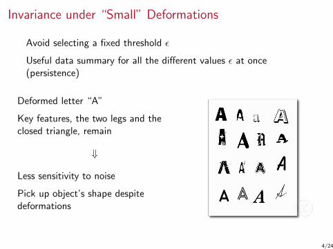
Invariance under “Small” Deformations

Avoid selecting a fixed threshold ε

Useful data summary for all the different values ε at once(persistence)

Deformed letter “A”

Key features, the two legs and theclosed triangle, remain

⇓

Less sensitivity to noise

Pick up object’s shape despitedeformations

4/24

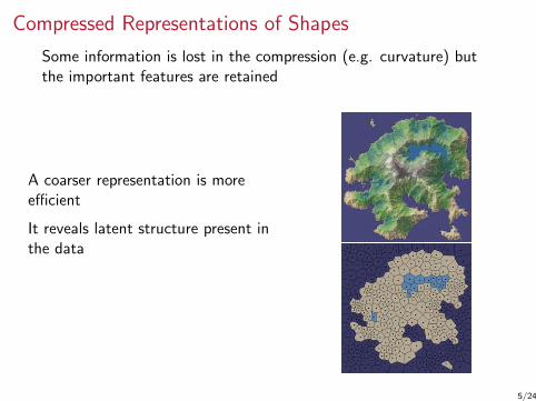
Compressed Representations of Shapes

Some information is lost in the compression (e.g. curvature) butthe important features are retained

A coarser representation is moreefficient

It reveals latent structure present inthe data

5/24

Agenda

Key Ideas in Topological Data Analysis (TDA)

Concept Analysis and Document Clustering

Detecting Significant Local Structural Sites in Proteins

Conclusions

Concept Analysis and Document Clustering [4,5]

I A high frequency and nearby keywordset (a concept) is asimplex

I Collection of simplexes represents the structure of concepts

Input: Collection of documents (each is a list of tokens or terms)

Aim:

1. Cluster documents based on the topology of concepts

2. Geometry is language-independent → Compare documentswritten in different languages

[4] Lin et al. IEEE ICDM Workshops, 412–416, 2006.

[5] Lin and Chiang. IEEE SMC 2006, 6:4763–4767, 2006.

6/24

Approach Outline

1. Extract keywords and keywordsets from documentsKeywordsets capture association semantics:

“Wall Street“ 6≡ “Wall“, “Street“

“White House“ 6≡ “White“, “House“

2. Build the simplicial complexEach simplex represents a concept

3. Cluster documents

7/24

Selecting Keywords for Document Representation

A keyword is an important tokenImportant token has high tfidf and support values

Definition (tfidf)

Let Tr denote the total number of documents. The tfidf of token ti ina document dj is

TFIDF(ti , dj) = tf(ti , dj) logTr

df(ti ).

tf – term frequency (frequency of ti in dj)

df – document frequency (documents with at least one occurrence of ti )

Definition (support)

support({t1, t2, . . . , tk}) is the number of documents that contain

t1, t2, . . . , tk within d tokens.

8/24

Background

Definition (n-simplex)

A n-simplex ∆(v0, v1, . . . , vn) is a set of abstract vertices {v0, v1, . . . , vn}.A q-subset of a n-simplex is called a q-face; q-simplex ∆(vj0 , . . . , vjq )

whose vertices are a subset of {v0, v1, . . . , vn}.

Definition (Abstract simplicial complex)

Finite set of simplexes C = (V ,S) such that:

I any set consisting of one vertex v ∈ V is a simplex,

I any face of a simplex s ∈ S is also in C (Closed condition).

Maximal simplex is not a face of any other simplex

9/24

Combinatorial Structure of Documents

Definition (Apriori condition)

Any q-subset of a n-keywordset is a q-keywordset for q ≤ n.

Keyword ≡ abstract vertex(q + 1)-keywordset ≡ abstract q-simplex of keywords

Lemma

The closed condition of abstract simplexes is the Apriori conditionof keywordsets and vice versa.

Theorem (Keyword simplicial complex)

Pair (Vtext, Stext) is an abstract simplicial complex:- Vtext is the set of keywords,- Stext is the set of keywordsets.

10/24

Semantic Language and the Model

L1 Idea is the semantic of whole keyword simplicial complex

L2 Basic concept B-concept(k) is the semantic of keyword k

L3 Intermediate concept I-concept(∆) is the semantic ofq-simplex ∆

L4 Primitive concept P-concept is the I-concept of amaximal simplex

L5 Component concept C-concept is the semantic of aconnected component

11/24

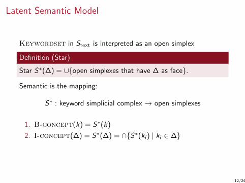
Latent Semantic Model

Keywordset in Stext is interpreted as an open simplex

Definition (Star)

Star S∗(∆) = ∪{open simplexes that have ∆ as face}.

Semantic is the mapping:

S∗ : keyword simplicial complex → open simplexes

1. B-concept(k) = S∗(k)

2. I-concept(∆) = S∗(∆) = ∩{S∗(ki ) | ki ∈ ∆}

12/24

Document ClusteringDocuments d , d1, d2

P-clustering by P-concept

d contains maximal simplex P-concept → Link(d , P-concept)

d1 and d2 are clustered together if both have the same maximal keywordset

C-clustering by C-concept

d contains simplex as part of C-concept → Link(d , C-concept)

d1 and d2 are clustered together if both have a keywordset in the sameC-concept

keywordsets w0 and wn are in the same connected component if consecutivetwo simplexes in w0,w1, . . . ,wn share a face

Relative clustering by (C-concept, sub-concept)

d contains I-concept ⊂ C-concept and I-concept 6⊂ sub-concept →Link(d , (C-concept, sub-concept))

d1 and d2 are not clustered together if only common topics are in sub-concept

13/24

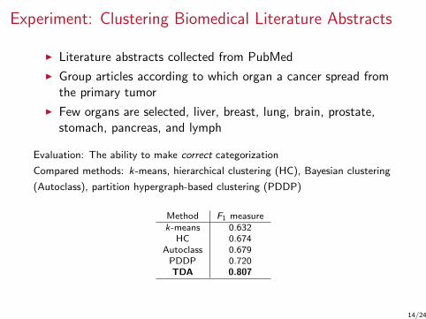
Experiment: Clustering Biomedical Literature Abstracts

I Literature abstracts collected from PubMed

I Group articles according to which organ a cancer spread fromthe primary tumor

I Few organs are selected, liver, breast, lung, brain, prostate,stomach, pancreas, and lymph

Evaluation: The ability to make correct categorization

Compared methods: k-means, hierarchical clustering (HC), Bayesian clustering

(Autoclass), partition hypergraph-based clustering (PDDP)

Method F1 measurek-means 0.632

HC 0.674Autoclass 0.679

PDDP 0.720TDA 0.807

14/24

Agenda

Key Ideas in Topological Data Analysis (TDA)

Concept Analysis and Document Clustering

Detecting Significant Local Structural Sites in Proteins

Conclusions

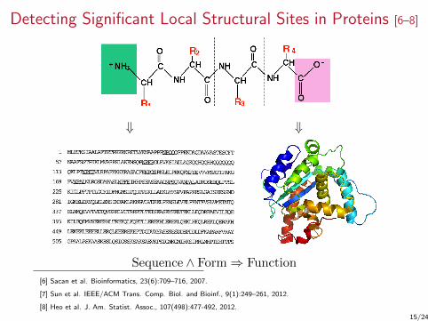
Detecting Significant Local Structural Sites in Proteins [6–8]

⇓ ⇓

Sequence ∧ Form⇒ Function

[6] Sacan et al. Bioinformatics, 23(6):709–716, 2007.

[7] Sun et al. IEEE/ACM Trans. Comp. Biol. and Bioinf., 9(1):249–261, 2012.

[8] Heo et al. J. Am. Statist. Assoc., 107(498):477-492, 2012.

15/24

Biological BackgroundGoal:

1. Identify protein family-specific local sites and associatedfeatures

2. Classify proteins based on extracted features

Definition (Protein site)

– A 3D location in the protein– Local spatial neighborhood with certain structure and function

Protein family – group of proteinsrelated by evolution, function orstructure

16/24

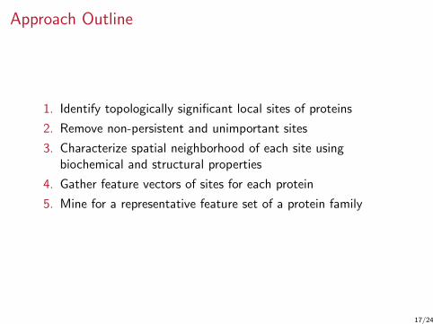
Approach Outline

1. Identify topologically significant local sites of proteins

2. Remove non-persistent and unimportant sites

3. Characterize spatial neighborhood of each site usingbiochemical and structural properties

4. Gather feature vectors of sites for each protein

5. Mine for a representative feature set of a protein family

17/24

Sampling of the Structural Centers

I Given protein P = {p1, p2, . . . , pn} as a set of Cα centers

I Distance function ΦP : R3 → R:

ΦP(x) = minpi∈P

dist(pi , x)

I ΦP describes the influence of P to neighboring space

I Proteins with similar structure have similar distance fields

Potential sites are critical points of ΦP

These are intersections between someDelaunay simplex and its dual Voronoielements

3.1 Sampling of the structural centers

Given a protein P as the set of its alpha Carbon (C!) atom centersP ! fp1, . . . ; png, the distance function !P : R3 ! R w.r.t. P is definedas follows: !P"x# is the nearest distance from x to any pi 2 P. !P

describes the influence of (the backbone atoms of ) protein P to itsneighboring space via the distance field. Intuitively, if two proteins havesimilar structure, they should have similar distance fields. In particular,if there are regions in space where proteins display similar localstructural patterns, then they should have similar distance fields inand around that region as well.We identify the potential motif centers by finding the critical points

of this distance function. Formally, critical points of a smooth functiong, are points with vanishing gradients. In our case, for a functiondefined over R3, there are four types of critical points: local minima,local maxima and two types of saddle points. Note that, when distanceto backbone atoms is used as function g, it turns out that the set ofcritical points of !P is the set of intersection points between someDelaunay simplex (a point, edge, triangle or tetrahedron) with its dualVoronoi elements (a polytope, face, edge, point, respectively) (Fig. 2),and can be computed in O"n2# time where n ! jPj (Giesen and John,2003).We now collect " as the set of critical points of the distance function.

Some examples of structural motifs that such critical points can captureare illustrated in Figure 3. The spatial neighborhood of a critical pointis defined as the spherical region centered at the critical point,whose radius is its distance function value.Following the generation of all critical points of distance, we perform

a filtering of these points to eliminate noise. The structural importanceof the critical points were assigned using the topological persistencealgorithm from Edelsbrunner et al. (2002), and those with smallpersistence were removed from". This topological method of removingnoise is fundamentally different from those that employ clustering ofneighboring points, in terms of the type of noise it removes. Roughlyspeaking, it measures the importance of a feature (critical point) bymeasuring how persistent this feature remains if the distance fieldis perturbed. Note that filtering based on persistence effectively

eliminates the noise inherent in the crystallography methods usedto obtain the atom coordinates. After the filtering step, the numberof remaining critical points are roughly the same as the numberof the amino acids in the protein.

3.2 Characterizing the spatial neighborhood

As a by-product of our structural center sampling method, we have anatural way to decide the neighborhood size, which is better thanprefixing some threshold value. For the spatial neighborhood aroundeach critical point, we associate a feature vector, based on both thestructural and biochemical nature of the neighborhood. The structuralfeatures include: the persistence value of the critical point, the radius ofthe neighborhood and the writhing number. The biochemical features weuse are based on the frequency and location of the constituent atomswithin the neighborhood.

The writhing number, or writhe, is originally used to measure thesupercoiling phenomenon for a space curve, and has been used tocharacterize both DNA (Fuller, 1978; Klenin and Langowski, 2000;Swigon et al., 1998) and protein structures (Levitt, 1983; Rogen andFain, 2003). We compute the writhe of those backbone pieces containedwithin the spatial neighborhood to measure their relative spatialarrangements.

In order to capture the biochemical nature of the spatial environ-ment, we use the frequencies of each of the side-chain carbon, nitrogen,oxygen and sulfur atoms within the spherical region. Furthermore,the location information of these atoms is captured by computing thecenter of mass for each atom type. Note that our framework can beeasily extended to use physico-chemical properties such as hydro-phobicity, solvent accessibility, Van der Waals radii or mobility, whichcan capture more detailed information about the spatial environment(Bagley and Altman, 1995). However, we did not use such extendedfeatures in this study, because of the computational cost they incurred.

3.3 Mining for a representative feature set

Each protein pi now has a set " ! fc1; . . . ; cng of feature vectorsgenerated from its important critical points. Let F ! fp1; . . . pmg denotea family of proteins that are known to share a common structural orfunctional property. And let the set G denote the rest of the proteinsin the dataset. We wish to determine the critical points that are uniqueto family F, and assess their ability to discriminate the proteins withinthe family from the rest of the proteins. Note that the algorithmto detect family-specific critical points has to allow changes in thevalues of the feature vectors. We utilized a distance-based approachfor this purpose.

Fig. 2. Delaunay tessellation (dashed lines) and Voronoi diagram(solid lines) of a set of points in 2D. Region enclosed by a Voronoipolyhedron is the area that is closest to the enclosed point than to anyother point in the set. Delaunay tesselation is obtained by connectingpoints that share a boundary. In 3D, Delaunay tessellation would givespace-filling tetrahedra. A circle (sphere) can be drawn whose center isa vertex of Voronoi diagram and which passes through the points inthe corresponding Delaunay triangle (tetrahedra).

(a) (b)

Fig. 3. Two types of motifs captured by critical points of the distancefunction. In (a), four pieces of protein backbone come close in space,forming a contact as indicated by the tetrahedron in the middle.The double point is a local maximum of !. In (b), the cross-point is asaddle point. Local spatial patterns can be captured by taking a ballcentered at these critical points.

711

Detecting protein functional sites

at National and U

niversity Library on June 26, 2013http://bioinform

atics.oxfordjournals.org/D

ownloaded from

18/24

Filtering of Critical Points for Noise

I Remove unimportant critical points

I Important features remain persistent if distance field isperturbed

I Persistence-based filtering removes noise inherent incrystallography methods used to get Cα

Critical points capturestructural motifs

3.1 Sampling of the structural centers

Given a protein P as the set of its alpha Carbon (C!) atom centersP ! fp1, . . . ; png, the distance function !P : R3 ! R w.r.t. P is definedas follows: !P"x# is the nearest distance from x to any pi 2 P. !P

describes the influence of (the backbone atoms of ) protein P to itsneighboring space via the distance field. Intuitively, if two proteins havesimilar structure, they should have similar distance fields. In particular,if there are regions in space where proteins display similar localstructural patterns, then they should have similar distance fields inand around that region as well.We identify the potential motif centers by finding the critical points

of this distance function. Formally, critical points of a smooth functiong, are points with vanishing gradients. In our case, for a functiondefined over R3, there are four types of critical points: local minima,local maxima and two types of saddle points. Note that, when distanceto backbone atoms is used as function g, it turns out that the set ofcritical points of !P is the set of intersection points between someDelaunay simplex (a point, edge, triangle or tetrahedron) with its dualVoronoi elements (a polytope, face, edge, point, respectively) (Fig. 2),and can be computed in O"n2# time where n ! jPj (Giesen and John,2003).We now collect " as the set of critical points of the distance function.

Some examples of structural motifs that such critical points can captureare illustrated in Figure 3. The spatial neighborhood of a critical pointis defined as the spherical region centered at the critical point,whose radius is its distance function value.Following the generation of all critical points of distance, we perform

a filtering of these points to eliminate noise. The structural importanceof the critical points were assigned using the topological persistencealgorithm from Edelsbrunner et al. (2002), and those with smallpersistence were removed from". This topological method of removingnoise is fundamentally different from those that employ clustering ofneighboring points, in terms of the type of noise it removes. Roughlyspeaking, it measures the importance of a feature (critical point) bymeasuring how persistent this feature remains if the distance fieldis perturbed. Note that filtering based on persistence effectively

eliminates the noise inherent in the crystallography methods usedto obtain the atom coordinates. After the filtering step, the numberof remaining critical points are roughly the same as the numberof the amino acids in the protein.

3.2 Characterizing the spatial neighborhood

As a by-product of our structural center sampling method, we have anatural way to decide the neighborhood size, which is better thanprefixing some threshold value. For the spatial neighborhood aroundeach critical point, we associate a feature vector, based on both thestructural and biochemical nature of the neighborhood. The structuralfeatures include: the persistence value of the critical point, the radius ofthe neighborhood and the writhing number. The biochemical features weuse are based on the frequency and location of the constituent atomswithin the neighborhood.

The writhing number, or writhe, is originally used to measure thesupercoiling phenomenon for a space curve, and has been used tocharacterize both DNA (Fuller, 1978; Klenin and Langowski, 2000;Swigon et al., 1998) and protein structures (Levitt, 1983; Rogen andFain, 2003). We compute the writhe of those backbone pieces containedwithin the spatial neighborhood to measure their relative spatialarrangements.

In order to capture the biochemical nature of the spatial environ-ment, we use the frequencies of each of the side-chain carbon, nitrogen,oxygen and sulfur atoms within the spherical region. Furthermore,the location information of these atoms is captured by computing thecenter of mass for each atom type. Note that our framework can beeasily extended to use physico-chemical properties such as hydro-phobicity, solvent accessibility, Van der Waals radii or mobility, whichcan capture more detailed information about the spatial environment(Bagley and Altman, 1995). However, we did not use such extendedfeatures in this study, because of the computational cost they incurred.

3.3 Mining for a representative feature set

Each protein pi now has a set " ! fc1; . . . ; cng of feature vectorsgenerated from its important critical points. Let F ! fp1; . . . pmg denotea family of proteins that are known to share a common structural orfunctional property. And let the set G denote the rest of the proteinsin the dataset. We wish to determine the critical points that are uniqueto family F, and assess their ability to discriminate the proteins withinthe family from the rest of the proteins. Note that the algorithmto detect family-specific critical points has to allow changes in thevalues of the feature vectors. We utilized a distance-based approachfor this purpose.

Fig. 2. Delaunay tessellation (dashed lines) and Voronoi diagram(solid lines) of a set of points in 2D. Region enclosed by a Voronoipolyhedron is the area that is closest to the enclosed point than to anyother point in the set. Delaunay tesselation is obtained by connectingpoints that share a boundary. In 3D, Delaunay tessellation would givespace-filling tetrahedra. A circle (sphere) can be drawn whose center isa vertex of Voronoi diagram and which passes through the points inthe corresponding Delaunay triangle (tetrahedra).

(a) (b)

Fig. 3. Two types of motifs captured by critical points of the distancefunction. In (a), four pieces of protein backbone come close in space,forming a contact as indicated by the tetrahedron in the middle.The double point is a local maximum of !. In (b), the cross-point is asaddle point. Local spatial patterns can be captured by taking a ballcentered at these critical points.

711

Detecting protein functional sites

at National and U

niversity Library on June 26, 2013http://bioinform

atics.oxfordjournals.org/D

ownloaded from

19/24

Characterizing Spatial Neighborhood of a Critical PointStructural and biochemical properties of neighborhood:

I persistence value of a critical pointI neighborhood radiusI writhing numberI frequencies of C , N, O and S atomsI hydrophobicityI Van der Wals radiiI center of mass for each atom type

The dissimilarity d!ci; cj" of any given two critical points can bedefined in terms of an appropriate distance function between theircorresponding feature vectors. We observed that a simple Euclideandistance measure on normalized feature vectors was sufficient indetecting family-specific structural centers. A weighted Euclideandistance, that can highlight varying contributions of the individualenvironment features could also be designed by optimizing the weightsagainst an objective function.

When comparing a critical point cx to a protein p, we take thedistance of cx to its closest match in p as defined with the distancefunction:

d!cx; p" # minfd!cx; c1", . . . ; d!cx; cn"g

where c1, . . . ; cn are the critical points of the protein p. Intuitively, if acritical point cx is part of a protein p, one would expect a very smallvalue for d!cx; p".

For each candidate critical point cx of the proteins in the family F, wecalculate its distance to all the proteins in the dataset. For an idealdiscriminative critical point, the distances to the proteins in F would beclustered at a minimal, whereas the distances to the rest of the proteins,G, would take upon higher values. We modeled this intuition bydefining the discrimination score s of a critical point as follows:

s!cx" #!!cx;G"

!1$ !!cx;F "" % !1$ "!cx;F;G""!1"

where !!cx;F" is the average distance of cx to proteins in the family F,

!!cx;F " # avg!d!cx; p 2 F "" !2"

and " is the number of background proteins that have adistance smaller than the maximum within-family distanced %!cx;F " # max!d!cx; p 2 F "".

"!cx;F;G" # count!d!cx; p 2 G" & d %!cx;F"" !3"

In Equation (1), !!cx;F " and !!cx;G" ensure that those criticalpoints that have small within-family distance and high out-of-familydistance get higher discrimination scores. The average distances alone,however, do not guarantee a clear separation of the family proteinsfrom the rest. The term " favors those critical points that can clusterthe family proteins with minimal number of out-of-family proteins.In other words, ! works to select features common to family, while "works to avoid features that cannot discriminate family proteins fromthe rest. Each term in the denominator is padded with 1 for numericalstability.

Using the discrimination scores, we obtain a set of critical pointsranked by the scores reflecting how representative they are for a givenfamily F. We refer the collection of the critical point features with theirassociated scores as the representative feature set of the family.

3.3.1 Classification modeling Let ! # fc1; . . . ; cng be the repre-sentative feature set of family F, with corresponding discriminativescores S # fs1; . . . ; sng and maximum within-family distancesD% # fd %

1; . . . ; d%ng. The membership score of a new protein p to the

family F is calculated as follows:

! p;F " # 1

n

X

i#1:::n

sid %i ' d!ci; p"d!ci; p"

!4"

The membership score , is dominated by the matching features thathave small distance and high representative scores. The numerator termin the summation in Equation (4) provides a threshold logic based onthe maximum within-family distances d *. Those features that matchthe protein with a distance smaller than d * contribute positively in themembership score, whereas those that have a greater distance arepenalized in the scoring. The overall membership score reflects howwell a protein matches a representative feature set. In a multi-family

classification scheme, the membership score ! p;F " can be used toassign the protein p to the closest family.

4 RESULTS

4.1 Experimental setup

All the experiments were conducted on a single processorPentium 4 PC with 2.8GHz CPU and 1GB main memory.The selection of centers via determination of critical centersof the distance function was implemented in Python and C,using CGAL (CGAL, 2006) computational geometry library;the feature extraction and mining methods were developedunder Matlab environment.The proteins used in this study were selected from the

representative ASTRAL (Brenner et al., 2000) dataset of SCOP1.69 (Murzin et al., 1995) with 540% sequence homology.There were a total of 7237 entries in the ASTRAL dataset.The one-time-only generation of critical points and their

corresponding feature vectors took 49 s on the average perprotein.

4.2 Mining functional sites

The success of LFM-Pro could be assessed by applying it toprotein families that have well-defined functional sites,and investigating whether the sites detected by LFM-Promatch the known functional sites in these proteins. Serineproteases are the most studied family of proteins, in the contextof structural motif extraction (Bagley and Altman, 1995;Huan et al., 2004, 2005 Milik et al., 2003; Wallace et al.,1996). We follow the tradition and also use serine proteases forthis study. The proteins were selected from the SCOP super-family (b.47.1.*) ‘trypsin-like serine proteases’, here on referredas the superfamily and included both prokaryotic (PSP: 10SCOP entries) and eukaryotic (ESP: 19 SCOP entries) proteins,which share the same catalytic site.The local site mining for the SP family took 30 s to complete.

Note that, with the same number of localities to compare,the subgraph mining methods may take several days tocomplete (Huan et al., 2005). Figure 4 shows the mapping of

Fig. 4. Mapping of the top-scoring sites onto Alpha-lytic protein (1ssx).The features were obtained by mining SP dataset against a random setof 200 background proteins. Left: Features 1, 2, 4 and 5 span theneighborhood of the catalytic triad, whereas feature 3 contains adistant disulfide bridge CYS189–CYS220. Right: A closer look intothe catalytic region spanned by features 1, 2, 4 and 5. The residueswhose side-chain atoms are contained within these sites are shown.

712

A.Sacan et al.

at National and U

niversity Library on June 26, 2013http://bioinform

atics.oxfordjournals.org/D

ownloaded from

20/24

Mining for Representative Feature SetGiven:

I set of feature vectors Π = {c1, c2, . . . , cn} for each protein

I protein family F = {p1, p2, . . . , pm}I set of background proteins G

Distance based approach determines:

I critical points specific to F

I their ability to discriminate between F and G

Compare critical point cx to protein p:

dist(cx , p) = minci∈p

dist(cx , ci )

Representative critical point cx :

dist(cx , p)� dist(cx , g), p ∈ F , g ∈ G

21/24

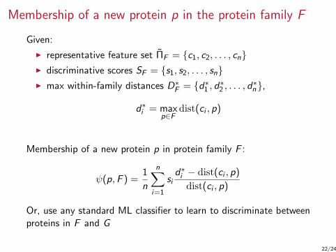
Membership of a new protein p in the protein family F

Given:

I representative feature set ΠF = {c1, c2, . . . , cn}I discriminative scores SF = {s1, s2, . . . , sn}I max within-family distances D∗F = {d∗1 , d∗2 , . . . , d∗n},

d∗i = maxp∈F

dist(ci , p)

Membership of a new protein p in protein family F :

ψ(p,F ) =1

n

n∑

i=1

sid∗i − dist(ci , p)

dist(ci , p)

Or, use any standard ML classifier to learn to discriminate betweenproteins in F and G

22/24

Experiment: Mining Functional Sites

Data set Method Features Accuracy

C1 DT 20,646 100AD 23,130 96

LFM-Pro 5,282 100

C2 DT 15,895 95AD 18,491 93

LFM-Pro 2180 100

C1 – clearly distinct families, C2 – closely related protein familiesDT – Delaunay tesselation, AD – Almost Delaunay

The dissimilarity d!ci; cj" of any given two critical points can bedefined in terms of an appropriate distance function between theircorresponding feature vectors. We observed that a simple Euclideandistance measure on normalized feature vectors was sufficient indetecting family-specific structural centers. A weighted Euclideandistance, that can highlight varying contributions of the individualenvironment features could also be designed by optimizing the weightsagainst an objective function.

When comparing a critical point cx to a protein p, we take thedistance of cx to its closest match in p as defined with the distancefunction:

d!cx; p" # minfd!cx; c1", . . . ; d!cx; cn"g

where c1, . . . ; cn are the critical points of the protein p. Intuitively, if acritical point cx is part of a protein p, one would expect a very smallvalue for d!cx; p".

For each candidate critical point cx of the proteins in the family F, wecalculate its distance to all the proteins in the dataset. For an idealdiscriminative critical point, the distances to the proteins in F would beclustered at a minimal, whereas the distances to the rest of the proteins,G, would take upon higher values. We modeled this intuition bydefining the discrimination score s of a critical point as follows:

s!cx" #!!cx;G"

!1$ !!cx;F "" % !1$ "!cx;F;G""!1"

where !!cx;F" is the average distance of cx to proteins in the family F,

!!cx;F " # avg!d!cx; p 2 F "" !2"

and " is the number of background proteins that have adistance smaller than the maximum within-family distanced %!cx;F " # max!d!cx; p 2 F "".

"!cx;F;G" # count!d!cx; p 2 G" & d %!cx;F"" !3"

In Equation (1), !!cx;F " and !!cx;G" ensure that those criticalpoints that have small within-family distance and high out-of-familydistance get higher discrimination scores. The average distances alone,however, do not guarantee a clear separation of the family proteinsfrom the rest. The term " favors those critical points that can clusterthe family proteins with minimal number of out-of-family proteins.In other words, ! works to select features common to family, while "works to avoid features that cannot discriminate family proteins fromthe rest. Each term in the denominator is padded with 1 for numericalstability.

Using the discrimination scores, we obtain a set of critical pointsranked by the scores reflecting how representative they are for a givenfamily F. We refer the collection of the critical point features with theirassociated scores as the representative feature set of the family.

3.3.1 Classification modeling Let ! # fc1; . . . ; cng be the repre-sentative feature set of family F, with corresponding discriminativescores S # fs1; . . . ; sng and maximum within-family distancesD% # fd %

1; . . . ; d%ng. The membership score of a new protein p to the

family F is calculated as follows:

! p;F " # 1

n

X

i#1:::n

sid %i ' d!ci; p"d!ci; p"

!4"

The membership score , is dominated by the matching features thathave small distance and high representative scores. The numerator termin the summation in Equation (4) provides a threshold logic based onthe maximum within-family distances d *. Those features that matchthe protein with a distance smaller than d * contribute positively in themembership score, whereas those that have a greater distance arepenalized in the scoring. The overall membership score reflects howwell a protein matches a representative feature set. In a multi-family

classification scheme, the membership score ! p;F " can be used toassign the protein p to the closest family.

4 RESULTS

4.1 Experimental setup

All the experiments were conducted on a single processorPentium 4 PC with 2.8GHz CPU and 1GB main memory.The selection of centers via determination of critical centersof the distance function was implemented in Python and C,using CGAL (CGAL, 2006) computational geometry library;the feature extraction and mining methods were developedunder Matlab environment.The proteins used in this study were selected from the

representative ASTRAL (Brenner et al., 2000) dataset of SCOP1.69 (Murzin et al., 1995) with 540% sequence homology.There were a total of 7237 entries in the ASTRAL dataset.The one-time-only generation of critical points and their

corresponding feature vectors took 49 s on the average perprotein.

4.2 Mining functional sites

The success of LFM-Pro could be assessed by applying it toprotein families that have well-defined functional sites,and investigating whether the sites detected by LFM-Promatch the known functional sites in these proteins. Serineproteases are the most studied family of proteins, in the contextof structural motif extraction (Bagley and Altman, 1995;Huan et al., 2004, 2005 Milik et al., 2003; Wallace et al.,1996). We follow the tradition and also use serine proteases forthis study. The proteins were selected from the SCOP super-family (b.47.1.*) ‘trypsin-like serine proteases’, here on referredas the superfamily and included both prokaryotic (PSP: 10SCOP entries) and eukaryotic (ESP: 19 SCOP entries) proteins,which share the same catalytic site.The local site mining for the SP family took 30 s to complete.

Note that, with the same number of localities to compare,the subgraph mining methods may take several days tocomplete (Huan et al., 2005). Figure 4 shows the mapping of

Fig. 4. Mapping of the top-scoring sites onto Alpha-lytic protein (1ssx).The features were obtained by mining SP dataset against a random setof 200 background proteins. Left: Features 1, 2, 4 and 5 span theneighborhood of the catalytic triad, whereas feature 3 contains adistant disulfide bridge CYS189–CYS220. Right: A closer look intothe catalytic region spanned by features 1, 2, 4 and 5. The residueswhose side-chain atoms are contained within these sites are shown.

712

A.Sacan et al.

at National and U

niversity Library on June 26, 2013http://bioinform

atics.oxfordjournals.org/D

ownloaded from

23/24

Agenda

Key Ideas in Topological Data Analysis (TDA)

Concept Analysis and Document Clustering

Detecting Significant Local Structural Sites in Proteins

Conclusions

Insightful Applications not Discussed in This TalkVisualization [9–11], Persistence perspective [12–14]

Advances in Arti!cial Neural Systems "

4436 84

(a)

4331 86

(b)

3836 83

(c)

3835 82

(d)

F#$%&' (: Mapper visualization of clusters in the neural network for theMiller-Reaven diabetes study data using 3 intervals with 25%overlap.From le) to right: clusters in the neural network a)er 12, 32, 57, and 107 epochs.*e neural network classi!cation is color coded with darkblue for overt diabetic (class −1), light blue/green for chemical diabetic (class 0), and dark red for not diabetic (class 1).

30

6

10

13

161

117

18

14

2565

1

(a)

316

9

131 1

1

12

15

13

151

118

68

(b)

1

2

2

152230

23

17

121 10

14 68

1

(c)

1

33

2

25

23

11

25 1

10

71

12

72

1

1

(d)

F#$%&' +:Mapper visualization of clusters in the neural network for theMiller-Reaven diabetes study data using 10 intervals with 50%overlap.From le) to right: clusters in the neural network a)er 12, 32, 57, and 107 epochs.*e neural network classi!cation is color coded with darkblue for overt diabetic (class −1), light blue/green for chemical diabetic (class 0), and dark red for not diabetic (class 1).the neural network andMapper results in Figures ( and +withthe PCA results in Figure , reveal that the cluster diagramandPCA results convey the same information in compressed (i.e.,clustered) and noncompressed ways, respectively.*us, theseresults serve to validate the cluster diagrams generated by aneural network and Mapper.

5. Conclusions

Neural networks and the Mapper method have a symbioticrelationship for solving clustering problems andmodeling thesolution. *e level sets of a neural network can be used tosolve a clustering problem for high-dimensional data sets,and the Mapper method can produce a low-dimensionalcluster diagram from these level sets that shows how theyare glued together to form a skeletal picture of the data set.Using neural networks and the Mapper method togethersimultaneously solves the problem that visualizing the levelsets of a neural network is di-cult for high-dimensional dataand the problem that the Mapper method only producesuseful results when applied to a function that solves aclustering problem e.ectively. Together, they combine thee-cacy of neural networks at solving clustering problems

with the clarity and simplicity of cluster diagrams producedby the Mapper method, thereby making the neural network’ssolution to the clustering problem much easier to interpretand understand. Further, the Mapper method allows theneural network’s solution to a clustering problem to be viewedat di.erent resolutions, which can help with developing amodel that shows important features at the right scale.

*e results of the case study provide evidence in supportof the conclusion that using a neural network to solve aclustering problem and the Mapper method to produce aclustering diagram is a valid means of producing an accuratelow-dimensional topological model for a data set. In particu-lar, the most important pattern observed in the scatterplot ofthe PCA results, which was progression classi!cations fromnon-diabetic (red +) to chemical diabetic (green ×) to overtdiabetic (blue ∘) in Figure ,, was also observed at a !nerresolution in the cluster diagram for the neural network inFigure +. Further, the linear chains of nodes connected byedges in the clustering diagrams in Figures ( and + provideda partial ordering on the neural network results that madethe results easier to interpret. In order to !rmly establish thevalidity of using a neural network with Mapper for a widevariety of applications, it is evident that in the future this

Mapper

PERSISTENT TOPOLOGY OF DATA 7

Theorem 2.3 ([22]). For a finite persistence module C with field F coe!cients,

(2.3) H!(C; F ) !=!

i

xti · F [x] "

"#!

j

xrj · (F [x]/(xsj · F [x]))

$% .

This classification theorem has a natural interpretation. The free portions ofEquation (2.3) are in bijective correspondence with those homology generatorswhich come into existence at parameter ti and which persist for all future parame-ter values. The torsional elements correspond to those homology generators whichappear at parameter rj and disappear at parameter rj + sj . At the chain level,the Structure Theorem provides a birth-death pairing of generators of C (exceptingthose that persist to infinity).

2.3. Barcodes. The parameter intervals arising from the basis for H!(C; F ) inEquation (2.3) inspire a visual snapshot of Hk(C; F ) in the form of a barcode. Abarcode is a graphical representation of Hk(C; F ) as a collection of horizontal linesegments in a plane whose horizontal axis corresponds to the parameter and whosevertical axis represents an (arbitrary) ordering of homology generators. Figure 4gives an example of barcode representations of the homology of the sampling ofpoints in an annulus from Figure 3 (illustrated in the case of a large number ofparameter values !i).

H0

H1

H2

!

!

!

Figure 4. [bottom] An example of the barcodes for H!(R) in theexample of Figure 3. [top] The rank of Hk(R!i) equals the numberof intervals in the barcode for Hk(R) intersecting the (dashed) line! = !i.

Barcodes[9] Pearson. Adv. in Art. Neu. Sys., 1–8, 2013.

[10] Nicolau et al. Proc. Natl. Acad. Sci., 108(17):7265–7270, 2011.

[11] Singh et al. Eur. Sym. on P.-B. Graph., 91–100, 2007.

[12] Chazal et al. ACM Sym. on Comp. Geom., 97–106, 2011.

[13] Adcock et al. ArXiv, 1210.0866, 2012.

[14] Chang et al. PLoS One, 91–100, 8(4):e58699, 2013.

24/24