topological quantum computing for beginners
TRANSCRIPT

Topological quantum computingfor beginners
John Preskill, CaltechKITP 7 June 2003http://www.iqi.caltech.edu/

http://www.theory.caltech.edu/~preskill/ph219/ph219_2004.html


Kitaev Freedman

Kitaev Freedman
Kitaev, Fault-tolerant quantum computation by anyons (1997).
Preskill and Ogburn, Topological quantum computation (1997).
Preskill, Fault-tolerant quantum computation (1997).
Mochon, Anyons from non-solvable groups are sufficient for universal quantum computation (2003).
Mochon, Anyon computers with smaller groups (2004).
Freedman, Larsen, and Wang, A modular functor which is universal for quantum computation (2000).
Freedman, Kitaev, and Wang, Simulation of topological field theories by quantum computers (2000).


Abstract for "Topological quantum computing for beginners," by John Preskill
I will describe the principles of fault-tolerant quantum computing, and explain why topological approaches to fault tolerance seem especially promising. A two-dimensional medium that supports abelian anyons has a topological degeneracy that can exploited for robust storage of quantum information. A system of n nonabelian anyons in two-dimensions has an exponentially large topologically protected Hilbert space, and quantum information can be processed by braiding the anyons. I will discuss in detail two cases where nonabelian anyons can simulate a quantum circuit efficiently: fluxons in a "nonabelian superconductor," and "Fibonacci anyons" with especially simple fusion rules.

Quantum Computation
Feynman ‘81 Deutsch ‘85 Shor ‘94
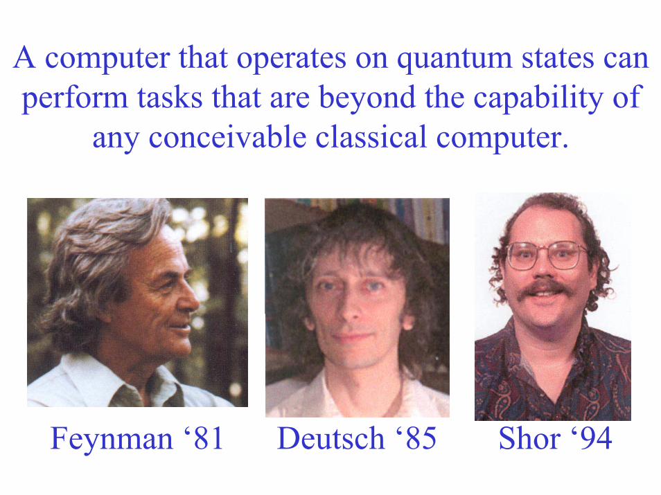
A computer that operates on quantum states can perform tasks that are beyond the capability of
any conceivable classical computer.
Shor ‘94Feynman ‘81 Deutsch ‘85

Finding Prime Factors1807082088687 4048059516561 64405905566278102516769401349170127021450056662540244048387341127590812303371781887966563182013214880557
= ? ?×

Finding Prime Factors1807082088687 4048059516561 64405905566278102516769401349170127021450056662540244048387341127590812303371781887966563182013214880557
39685999459597454290161126162883786067576449112810064832555157243
45534498646735972188403686897274408864356301263205069600999044599
×=
Shor ‘94

Quantum computer: the model(1) Hilbert space of n qubits: spanned by
Important: the Hilbert space is equipped with a natural tensor-product decomposition into subsystems.
Physically, this decomposition arises from spatial locality. Elementary operations (“quantum gates”) that act on a small number of qubits (independent of n) are “easy;” operations that act on many qubits (increasing with n) are “hard.”
(2) Initial state:
( )2n
= CH
22 2 2 2
times
n
n
= ⊗ ⊗ ⊗ ⊗C C C C C
| 000 0 | 0 n⊗⟩ = ⟩…
{ }1 2 1 0| | | | | , 0,1 nn nx x x x x x− −⟩ = ⟩⊗ ⟩ ⊗ ⊗ ⟩⊗ ⟩ ∈
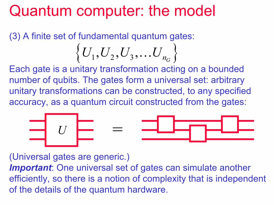
Quantum computer: the model(3) A finite set of fundamental quantum gates:
Each gate is a unitary transformation acting on a bounded number of qubits. The gates form a universal set: arbitrary unitary transformations can be constructed, to any specified accuracy, as a quantum circuit constructed from the gates:
(Universal gates are generic.)Important: One universal set of gates can simulate another efficiently, so there is a notion of complexity that is independent of the details of the quantum hardware.
{ }1 2 3, , ,GnU U U U…
U =

Quantum computer: the model(4) Classical control:
The construction of a quantum circuit is directed by a classicalcomputer, i.e., a Turing machine. (We’re not interested in what a quantum circuit can do unless the circuit can be designed efficiently by a classical machine.)
(5) Readout:
At the end of the quantum computation, we read out the result by measuring , i.e., projecting onto the basis
(We don’t want to hide computational power in the ability to perform difficult measurements.)
zσ { }| 0 ,|1⟩ ⟩

Quantum computer: the modelClearly, the model can be simulated by a classical computer with access to a random number generator. But there is an exponential slowdown, since the simulation involves matrices of exponential size.
(1) n qubits(2) initial state(3) quantum gates(4) classical control(5) readout
The quantum computer might solve efficiently some problems that can’t be solved efficiently by a classical computer. (“Efficiently” means that the number of quantum gates = polynomial of the number of bits of input to the problem.)

Quantum Error Correction
Shor ‘95 Steane ‘95
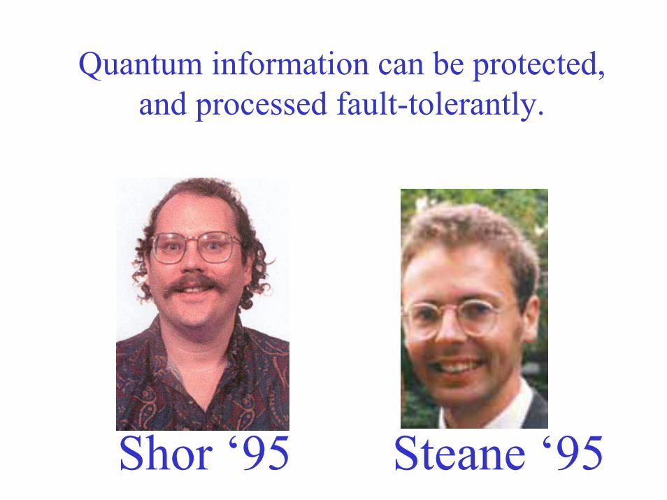
Quantum information can be protected,and processed fault-tolerantly.
Shor ‘95 Steane ‘95

QuantumComputer
EnvironmentDecoherence
If quantum information is cleverly encoded, it can be protected from decoherenceand other potential sources of error. Intricate quantum systems can be accurately controlled.
ERROR!

Two Physical SystemsWhat is the difference between:
A: Human B: Chip
Reliable hardware.Imperfect hardware. Hierarchical architecture with error correction at all scales...
Information processing prevents information loss.

Topology
Noisy
Gate
Quantum
Gate

Topological quantum computation (Kitaev ’97, FLW ‘00)
timecreate pairs
braid
braid
braid
annihilate pairs?
Kitaev
Freedman

Topological quantum computation (Kitaev ’97, FLW ‘00)
time
Physical fault tolerance with nonabelian anyons:
uncontrolled exchange of quantum numbers will be rare if particles are widely separated, and thermal anyons are suppressed...

Models of (nonabelian) anyonsA model of anyons is a theory of a two-dimensional medium with a mass gap, where the particles carry locally conserved charges. We define the model by specifying:
1. A finite list of particle labels {a,b,c,…}. These indicate the possible values of the conserved charge that a particle can carry. If a particle is kept isolated from other particles, its label never changes. There is a special label “0” – indicating trivial charge, and a charge conjugation operator C: a ¨ a (where 0=0). (Note: for “particle” you may read “puncture.”)
2. Rules for fusing (and splitting). These specify the possible values of the charge that can result when two charged particles are combined.
3. Rules for braiding. These specify what happens when two neighboring particles are exchanged (or when one is rotated by 2π).
a1 a2 a3 a4 an

Fusioncab
ca b N c b a× = = ×∑
0c cab ba abcV V V≅ ≅ ≅
Fusion rules:
Fusion vector space:
a b
c
dim( )c cab baV N≅
a b
c
µ
c
a b
µ(µ = 1, 2, 3,…, Nabc) ≅

Fusioncab
ca b N c b a× = = ×∑
0c cab ba abcV V V≅ ≅ ≅
Fusion rules:
Fusion vector space:
a a
0
dim( )c cab baV N≅
a 0
a
a
0
a
≅The charge 0 fuses trivially, and a is the unique label that can fuse with ato yield charge 0.

Fusion
Then there is a “topological Hilbert space” that can encode nontrivial quantum information. This encoding is nonlocal; the information is a collective property of the two anyons, not localized on either particle. When the particles with labels a and b are far apart, different states in the topological Hilbert space look identical to local observers. In particular, the quantum states are invulnerable to decoherence due to local interactions with the environment. That is why we propose to use this encoding in a quantum computer.
An anyon model is said to be nonabelian if for some a, and b,
a b
c
dim( ) 2.c cab bacc
V N⊕ ≅ ≥∑
a b
c
µ

Fusiona b
c
a b
c
µ
When we hide the quantum state from the environment, we hide it from ourselves as well! But, when we are ready to read out the quantum state (for example, at the conclusion of a quantum computation), we can make the information locally visible again by bringing the two particles together, fusing them into a single object. Then we ask, what is this object’s label? In fact, it suffices (for universal quantum computation) to be able to distinguish the label c = 0 from c ∫ 0. It is physically reasonable to suppose that we can distinguish annihilation “into the vacuum” (c = 0) from a lump that is unable to decay because of its conserved charge (c ∫ 0).

Abelian vs. nonabelianAbelian anyon models can also be used for robust quantum memory, e.g., a model of 2 fluxons and their dual 2 charges. A qubit is realized because the 2 flux in a hole can be either trivial or nontrivial (the information is carried by the labels themselves, not by the fusion states). This information is hidden from the environment by making the holes large and keeping them far apart (to prevent flux from tunneling from one hole to another, or to the outside edge, and to prevent the world lines of charges from winding about holes). -- Kitaev (1996)
However, this information may not be harder to read out. We’d need to contract a hole to see if a particle appears, or perform a delicate interference experiment to detect the flux, or …
Alternatively, by mixing the 2 with electromagnetic U(1), we might do the readout via a Senthil-Fisher type experiment (i.e., one that would actually work)! -- Ioffe et al. (2002)
Anyway, with nonabelian anyons we can exploit topology not just to store quantum information, but also to process it!

Associativity of fusion: the F-matrixa b c ( ) ( )a b c a b c× × = × ×
a b
µ
ν
c
d
ν ′
µ′
a b c
( ) ' ' '
' '
edabc e
eF
µ ν
µνµ ν ′
= ∑e e’
d
There are two natural ways to decompose the topological Hilbert space of three anyons in terms of the fusion spaces of pairs of particles. These two orthonormal bases are related by a unitary transformation, the F-matrix.
dabcV
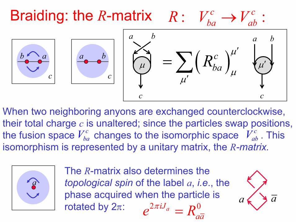
Braiding: the R-matrix : :c cba abR V V→
a b
c
µ
a b
c
µ′( )cbaR
µ
µµ
′
′
= ∑b a
c
a b
c
When two neighboring anyons are exchanged counterclockwise, their total charge c is unaltered; since the particles swap positions, the fusion space changes to the isomorphic space . This isomorphism is represented by a unitary matrix, the R-matrix.
cbaV c
abV
The R-matrix also determines the topological spin of the label a, i.e., the phase acquired when the particle is rotated by 2π: 2 0aiJ
aae Rπ =a
a
a

Models of (nonabelian) anyonsA model of anyons is a theory of a two-dimensional medium with a mass gap, where the particles carry locally conserved charges. We define the model by specifying:
1. A finite label set {a,b,c,…}.2. The fusion rules3. The F-matrix (expressing associativity of fusion).4. The R-matrix (braiding rules).
These determine a representation of the mapping class group (braiding plus 2π rotations), and define a unitary topological modular functor (UTMF), the two-dimensional part of a (2+1)-dimensional topological quantum field theory (TQFT) ---related to a (1+1)-dimensional rational conformal field theory (RCFT).
a1 a2 a3 a4 an
cabc
a b N c× = ∑

Example: Yang-Lee (Fibonacci) Model
1 1
0 or 1
The charge takes two possible values: 0 (trivial) and 1 (nontrivial, and self-conjugate). Anyonshave charge 1.Two anyons can “fuse” in either of two ways: 1 1 0 1× = +
This is the simplest of all nonabelian anyon models. Yet its deceptively simple fusion rule has profound consequences.
In particular, the fusion rule determines the F-matrix and R-matrix uniquely; the resulting nontrivial braiding properties are adequate for universal quantum computation (pointed out by Kuperberg).

Suppose n anyons have a trivial total charge 0.What is the dimension of the Hilbert space?
Nonabelian Anyons: Yang-Lee model 1 1
0 or 1
1
1
0,1
1
0,1
1
0,1
1
0,1
1
0,1
1
0,1
1 1
10,1
The distinguishable states of n anyons (a basis for the Hilbert space) are labeled by binary strings of length n-3.
1
1
0
1
0
1
1But it is impossible to have two zeros in a row:

Suppose n anyons have a trivial total charge 0.What is the dimension of the Hilbert space?
Nonabelian Anyons: Yang-Lee model 1 1
0 or 1
1 1
10,1 0,1
1
0,1
1
0,1
1
0,1
1
0,1
1 1
10,1
The distinguishable states of n anyons (a basis for the Hilbert space) are labeled by binary strings of length n-3.
1
1
0
1
0
1
1But it is impossible to have two zeros in a row:
Therefore, the dimension is a Fibonacci number:
Asymptotically, the number of qubits encoded by each anyon is:2, 3, 5, 8, 13, 21, 34, 55, 89, ...D =
( )2 2 2log log 1 5 / 2 log (1.618) .694φ = + = =

Nonabelian Anyons: Yang-Lee model 1 1
0 or 1
We say that d = φ is the (quantum) dimension of the Fibonacci anyon…
This counting vividly illustrates that the qubits are a nonlocal property of the anyons, and that the topological Hilbert space has no particularly natural decomposition as a tensor product of small subsystems.
Anyons have some “nonlocal” features, but they are not so nonlocal as to profoundly alter the computational model (the braiding of anyons can be efficiently simulated by a quantum circuit)…
( )2 2 2log log 1 5 / 2 log (1.618) .694φ = + = =
Asymptotically, the number of qubitsencoded by each anyon is:
1 1 1 1 1

The quantum dimension
aa
Every anyon label a has a quantum dimension, which we may define as follows: Imagine creating two particle-antiparticle pairs, and then fusing the particle from one pair with the antiparticle of the other… aa
1,= 1
ad=
Annihilation occurs with probability 1/da2. This is a natural
generalization of the case where the charge is an irreducible representation R of a group G, where the “quantum dimension” is just the dimension |R| of the representation (which counts the number of “colors” going around the loop). But there is no logical reason why a dimension defined this way must be can integer, and in general it isn’t an integer.

The quantum dimensionThere is a more convenient normalization convention for particle-antiparticle pairs... a
a
Each time we add another tooth to the saw, it cost us another factor of 1/da.
a
a
We can compensate for that factor by weighting each pair creation or annihilation even by a factor of . ad
ad
ad
ad
ad
ad
ad
a
With this convention, a closed loop has weight a , as though we were counting colors…adad=
Now we can deform the world line of a particle (e.g., adding and removing “teeth”) without altering the value of a diagram.
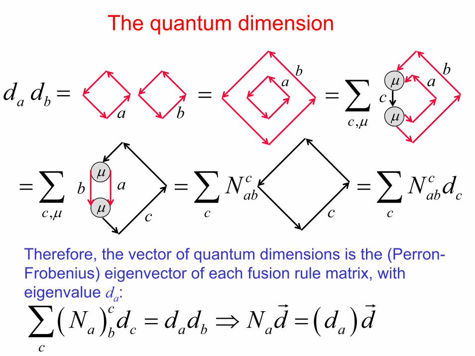
The quantum dimension
ab
a b
abµ
µ c c
a bd d = = ab
µ
µc
,c µ
= ∑
,c µ
= ∑ cab
cN= ∑ c
ab cc
N d= ∑
Therefore, the vector of quantum dimensions is the (Perron-Frobenius) eigenvector of each fusion rule matrix, with eigenvalue da:
( ) ( )ca c a b a ab
cN d d d N d d d= ⇒ =∑
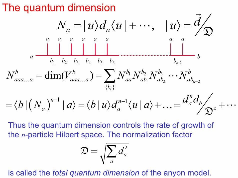
The quantum dimension
| | , |a adN u d u u= ⟩ ⟨ + ⟩ = D
a
a
b1
a
b2 b3
a
b4
a
b5
a
b6
a
bn-2
a
b
a
( )
31 2
1 2 2{ }
1 1
dim( )
| | | |
ni
bb b bb baaa a aaa a aa ab ab ab
bnn n a b
a a
N V N N N N
d db N a b u d u a
−
− −
= =
= ⟨ ⟩ = ⟨ ⟩ ⟨ ⟩ + = +
∑… …
… 2DThus the quantum dimension controls the rate of growth of the n-particle Hilbert space. The normalization factor
2a
ad∑D=
is called the total quantum dimension of the anyon model.

The quantum dimension
a b
cWhat if we create pairs of different types, and then fuse?
µ
= ∑ abµ
µ c ccabN= c
ab cN d=
ab
µ
µc( ) ( )a bd d p ab c
µ
→ = ∑
( )cab c
a b
N dp ab c d d⇒ → =
(generalizes what we found for the case b = a …)
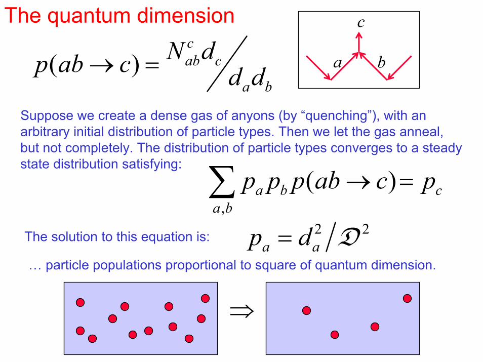
The quantum dimension
a b
c
( )cab c
a b
N dp ab c d d→ =
Suppose we create a dense gas of anyons (by “quenching”), with an arbitrary initial distribution of particle types. Then we let the gas anneal, but not completely. The distribution of particle types converges to a steady state distribution satisfying:
⇒
,
( )a b ca b
p p p ab c p→ =∑
… particle populations proportional to square of quantum dimension.
2 2a ap d= DThe solution to this equation is:

Braiding: the B-matrixFor the n-anyon Hilbert space, we may use the standard basis:
: :d dacb abcB V V→
a1
a2
b1
a3
b2 b3
a4
b4
a5
b5
a6
b6
a7
bn-2
an-1
b
an
The effect of braiding can be expressed in this basis:b c
a de
a d
b c
e’
( ) ' '
' '
edabc e
eB
µ ν
µνµ ν
′
′
= ∑And … the matrix B is determined by R and F:
F→ R→1F −
→

Topological quantum computation (Kitaev ’97, FLW ‘00)
timecreate pairs
braid
braid
braid
annihilate pairs?
Kitaev
Freedman

Topological quantum computation1. Create pairs of particles of specified types.2. Execute a braid.3. Fuse neighboring particles, and observe whether they annihilate.
Claim: This process can be simulated efficiently by a quantum circuit.
Need to explain:1. Encoding of topological Hilbert space.2. Simulation of braiding (B-matrix as a two-qudit gate).3. Simulation of fusion (F-matrix plus a one-qudit projective measurement).
a1
a2
b1
a3
b2 b3
a4
bn-3
an-2
an
an-1 ( ) ( 2)0
, ,
n
abca b cV
⊗ −
⊆ ⊕
dH0
, ,abc
a b cd N= ∑
Although the topological vector spaces are not themselves tensor products of subsystems, they all fit into a tensor product of d-dimensional systems, where this qudit is the “total fusion space” of three anyons…

Topological quantum computation
a1
a2
b1
a3
b2 b3
a4
bn-3
an-2
an
an-1
( ) ( 2)nd
⊗ −⊆ H
But what are R and Fin this model?
Therefore, the topological model is no more powerful than the quantum circuit model. But is it as powerful? The answer depends on the model of anyons, and in particular on the properties of the R-matrix and F-matrix.
To simulate a quantum circuit, we encode qubits in the topological vector space, and use braiding to realize a set of universal quantum gates acting on the qubits.
That is, the image of our representation of the braid group Bn on n strands should be dense in SU(2r), for some r linear in n.
Example: in the Fibonacci model, we can encode a qubit in the two-dimensional Hilbert space of four anyons with trivial total charge.0
1111V
1
1
a
1
1{ }0,1a ∈
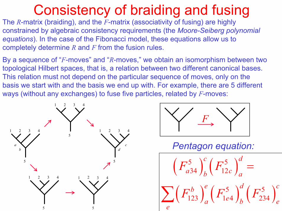
Consistency of braiding and fusingThe R-matrix (braiding), and the F-matrix (associativity of fusing) are highly constrained by algebraic consistency requirements (the Moore-Seiberg polynomial equations). In the case of the Fibonacci model, these equations allow us to completely determine R and F from the fusion rules.
By a sequence of “F-moves” and “R-moves,” we obtain an isomorphism between two topological Hilbert spaces, that is, a relation between two different canonical bases. This relation must not depend on the particular sequence of moves, only on the basis we start with and the basis we end up with. For example, there are 5 different ways (without any exchanges) to fuse five particles, related by F-moves:
1 2 3 4
5
ab d
1 2 3 4
5
c
1 2 3 4
5
1 2 3 4
5
1 2 3 4
5
F
Pentagon equation:
( ) ( )( ) ( ) ( )
5 534 12
5 5123 1 4 234
c d
a cb ae d cb
ea b ee
F F
F F F
=
∑

Consistency of braiding and fusing
( ) ( ) ( )4 4 4 4123 1 231 12 213 13
b c ca cba b a
bF R F R F R=∑
F
R
1 2 3
4
b
1 2 3
4
a
2 3 1
4
b2 3 1
4
c
2 1 3
4
c
2 1 3
4
a
F R F
FR R
Hexagon equation:
Furthermore, if the pentagon and hexagon equations are satisfied, then all sequences of F- and R-moves from an initial basis to a final basis yield the same isomorphism!
A systematic (in principle) procedure for constructing anyon models:1. Assume a fusion rule.2. Solve pentagon and hexagon equations for R and F.
-- If no solutions, the fusion rules are incompatible with local quantum physics.
-- If multiple solutions, each is a valid model.

Example: Fibonacci model
1
1 1 1
b
1
1 1 1
a = Σb Fab
1 1
aRa:
( )4 /5
2 /5
0, , 5 1 / 2 1
0
i
i
eF R
e
π
π
τ ττ φ
τ τ
= = = − = − −−
This solution is unique (aside from freedom to redefine phases and take the parity conjugate). Furthermore, products of the
1 1 1
1
a
1 1 1
1
b
noncommuting matrices R and FRF-1
(representing the generators of the braid group B3) are dense in SU(2).

Example: Fibonacci model
We encode a qubit in four anyons. To simulate a quantum circuit, we need to do (universal) two-qubit gates.
1 1 1
1
a
1 1 1
1
b
The two-qubits are embedded in the 13-dimensional Hilbert space of eightanyons.
The representation of B13 determined by our R and F matrices is universal – i.e., dense in SU(13), so in particular we can approximate any SU(4) gate arbitrarily well with some finite number of exchanges. If we fix accuracy of the approximation to the gate, we can use quantum error- correcting codes and fault-tolerant simulation to perform an efficient and reliable quantum computation.
Here quantum-error correction might be needed to correct for the (small) flaws in the gates, but not to correct for storage errors.
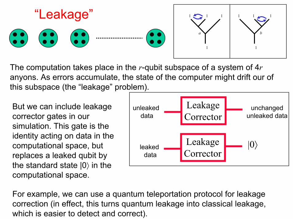
“Leakage”
The computation takes place in the r-qubit subspace of a system of 4ranyons. As errors accumulate, the state of the computer might drift our of this subspace (the “leakage” problem).
1 1 1
1
a
1 1 1
1
b
LeakageCorrector
LeakageCorrector
unleakeddata
unchangedunleaked data
leaked data
|0⟩
But we can include leakage corrector gates in our simulation. This gate is the identity acting on data in the computational space, but replaces a leaked qubit by the standard state |0⟩ in the computational space.
For example, we can use a quantum teleportation protocol for leakage correction (in effect, this turns quantum leakage into classical leakage, which is easier to detect and correct).

Topological quantum computation
To summarize, we can simulate a universal quantum computer using (for example) Fibonacci anyons, if we have these capabilities:
1. We can create pairs of particles.2. We can guide the particles along a specified braid.3. We can fuse particles, and distinguish complete annihilation from incomplete annihilation.
-- The temperature must be small compared to the energy gap, so that stray anyons are unlikely to be excited thermally.
-- The anyons must be kept far apart from one another compared to the correlation length, to suppress charge-exchanging virtual processes, except during the initial pair creation and the final pair annihilation.

a b
c
µ
F
R
(Nonabelian) anyonsAn anyon model is characterized by its label set, fusion rules, F-matrix, and R-matrix.
Classifying the models (finding all solutions to the pentagon and hexagon equations) is an important (hard) unsolved mathematical problem.We know how to find some examples (e.g., Chern-Simons theories), but we don’t know how rich the possibilities are.
Such a classification would be an important step toward classifying topological order in two dimensions.
There would still be more to do, though … For example, this would be a classification of gapped two-dimensional bulk theories, and one bulk theory can correspond to more than one (1+1)-dimensional theory describing edgeexcitations. And of course, we would like to know, both for practical and theoretical reasons, whether the model can be realized robustly with some local Hamiltonian (and how to realize it).

Topological quantum memory Kitaev ‘96Qubits can reside in holes in a planar array, where the holes carry Z2charge or flux. Then the quantum memory is topologically stable, but nontopological couplings between holes are needed to complete a set of universal gates.
This scheme might be realizable in suitably designed Josephson-junction arrays, which have a phase that can be interpreted as a condensate of objects with charge 4e. A hole in the array can carry charge 2e or flux Φ0/2=2π/4e. Ioffe et al. ‘02

Quantum many-body physics:Exotic phases in optical lattices
Atoms can be trapped in an optical lattice. The lattice geometry and interactions between neighbors can be chosen by the “material designer” (direction-dependent and spin dependent tunneling between sites).
In particular, Duan, Lukin, and Demler (cond-mat/0210564) have described how Kitaev’s honeycomb lattice model, which supports nonabelian anyons, can be simulated using an optical lattice.

Topological quantum computingfor beginners
John Preskill, CaltechKITP 7 June 2003http://www.iqi.caltech.edu/