1

Topology Identification of SmartMicrogridsBof Nicoletta,Michelotti Davide, Muraro Riccardo

I . INTRODUCTION

A. Pratical relevanceof theproblem

The widely useof distributedenergygeneration(solar pan-els, wind turbines,etc), the presenceof loads with significantenergyconsumption (electric cars)andthe needfor reliabilityof energysupply in critical areas has led the emergence ofSmart Grid (SG), which can act in real time to managethepower grid in an efficient manner, concerning various aspectsand features. Several studies in this area have been madeand are still under progress (optimization of consumption,reduction of waste energy, detection of faults and maliciusattacks, etc), neverthelessthe knowledge of the physical gridstructure is a basicingredient in all thesestudies.

Figure 1. Hierarchy in energy dispatching: from transmission high-voltagepower to distribution medium-low voltagepower network.

As a matter of fact, knowing the arrangement ofloads/generators on transmissionlines is essential in order tomakeefficient electricity dispatchment,avoiding energywasteandvoltagedrops. In addition, through the knowledge of thisgraph is possible to implement a scheduling of connecteddevices to avoid overload of the lines. Depending on thecontext, the knowledge we have on grid topology is notalways exhaustive. Surely the low voltage grid topology isin general not known, and nowadays there is no need ofthis knowledge since there is no practical interest due tothe fact that it is not properly monitored. Since in futuregrid development PMUs devices will probably beenwidelyused, the knowledgeof grid topology will give importantinformation for the optimization of electricity dispatchment.Moreover the networkknowledgeis even more relevant withthe increasingcomplexity of networks,in which agents arenot consideredexclusively passive loadsbut can constitute asource of energythrough common microgeneration devices.

B. Objectiveandtranslationof theproblem

This study of predominantly theorical-simulation kind tryto providea static estimation algorithm for the identificationof network topology of smart microgrids. The grid graphtopology canbethought fixedduring thecomputationtimeandin this senseit is a staticestimation. We consider “microgrid”as the smallestportion available of the low-voltage powerdistribuition network that is managedautonomously from therest of the network,having all the characteristics of interest.We assumethat dataandinformation of the grid areobtainedfrom a networkof PhasorMeasurementUnits (PMU’s).

Each node of the grid is supposed to be a PMU thatunder certain hypothesisprovidesanglemeasurementsprob-abilistically distributed as a Gaussianrandom variable [1].Therefore theelectrical networkcanberegardedasa Gaussianprobabilistic model. Due to this probabilistic model, we cangive a graphical representation of the conditional dependenceof measures, obtaining a graph which have a node for eachPMU and represent the conditional dependences of nodes.This type of analysis is known as graphical models, and isbasedon the relationship existing between the concentrationmatrix (inverse of the sample covariance matrix) and theconnections within the nodes in the graph. As a matter offact the concentration matrix is sparseandnon-zero elementsimply theexistenceof a link betweenthecorrespondingnodesof the graphical representation.

According to thepropertiesof theelectric network,thecon-centrationmatrix contains not only elements referring to linksbetween adjacent nodes, but also thosereferring to second-neighbours. The sameinformation is given by the sparsityof the square Laplacian matrix of the electrical network.Due to this, and starting from the graph identified using theconcentration matrix, a procedure to find only first-neighboursis needed. In theory (and under certain assumptions) someprocedureswhich allow to determine the only root of a graphexist.Howeverthesedonot suitsour problembecausewehaveonly an estimator of the correlation matrix andthe latter doesnot have exactlythesamesparsityasL2(if L is theLaplacian). A different technique has then beenelaborated to find theactual electrical graph, a technique mainly basedon the factthat power grid hasa treestructure.

In practice, known a seriesof measurements madeon pnodes of theelectric graph,at first we computethesampleco-variancematrix andthen, usingtechniquestypical of graphicalmodel we obtain an estimation of the topology of the graph,which will be further elaborated to obtain a tree structurefor the graph itself. It is evident that the resulting graphregards interconnections between the PMU devices arrangedon thenetworkthatprovides anapproximation of thephysicalstructure of power grid that underlies.

2

C. Stateof art

At present there is no study that tries to solve the spe-cific problem of power smart grid graph identification. Manyaspects of the problem are basedon typical approachescon-cerning graphical models which can be applied to electricalnetwork too.

Ming Yuan and Yi Lin in their article [2] focus attentionon selection andestimation of the the concentration matrix inGaussiangraphical model usingpenalized likelihood methods.The two provided methods they called lasso-type estimatorand nonnegative garrote-typeestimator lead to a sparseandshrinkage estimator of the concentration matrix and thusconduct model selectionand estimationsimultaneously. Theimplementation of this two methods can be done effectivelyby taking advantageof the efficient maxdet algorithm devel-oped in convex semidefinite optimization. The competitiveperformance they proposedbetween two methods show thatgarrote-typeestimatorgiving advantagefor model-fitting whena goodinitial estimator is availableashappensin our purposeof power grid.

Massive amount of measurements and their transmissionacrossthe grid by modern information technology makethegrid prone to attacks. Hanie Sedghi and Edmond Jonckheerein their article[1] try to solvetheproblemof themostdreadedcyber-attacks on the electrical infrastructure rappresented by“false data injection” that compromises the PMU’s data.Inadvertently they reveal somefundamental concepts usefulfor identification of power grid topology exploiting condi-tional mutual information in GaussianMarkov RandomField(GMRF). Therefore they explore the neighboring propertyof PMU angle measurements, then useso-called ConditionalCovariance Test (CCT) on PMU angle measurements andshow that,becauseof the walk-summability of grid graph, theoutput of CCT follows the grid topology. In fact, when thesystemis under falsedatainjection attack, the output of CCTmethod missessomelines that are present in the grid graph.The approachusedin this work hasprovento be the closestto the problemof grid topology identification eventhough forotherpurposesandotherpoint of view.

D. Ourcontribution

Starting from the power grid model suggested in [3], wereformulate the problem of graphical model selection forthe purpose of grid topology identification. To do this wecomputed the theoretical sample covariance matrix of thepower grid model. From its inverse,represented by the con-centrationmatrix, we obtainedsomeproperties thatthis sparsematrix musthave from theorical point of view. We have alsofound a relationshipbetween theconcentrationmatrix andtheLaplacian matrix under some hypothesisand exploited thisrelation as much as we could to obtain information whichcould help in the reconstruction of the electric graph.

We introduced the penalized likelihood algorithm givenby garrote-type estimator [2] on the concentration matrixobtained from power grid model. The problem of the tuningparameter, necessary for using garrote type estimator hasnotbeen completely solved yet, but applying our second step

algorithm to reconstruct the likliest electrical tree, the choiceof the tuning parameterdoes not seemcritical.

E. Summary

SectionII providesthe mathematicalpreliminary andmainnotationsusedfor thedescription of a graph relating a electricgrid. Thefoundamentalresultrefersto theapproximatemodelof microgrid proposedin [3] that constitutes the basis forthe following sections. SectionII I introducesthe main ideasof graphical models and it provides someproperties of themodelled power grid. Thevariousaspectsconsidered here canbe summarized in: first and secondneighbours dipendencebetween nodes, relation between Laplacian matrix and con-centration matrix, explanationof garrote-type estimator. Thegoalscollected in SectionIV aretwofold: first it provides thenotion of bipartite graph and brings back the algorithm SBN(Squaredof Bipartitegraphswith a specifiedNeighbourhood),subsequently it explainesour algorithm for the determinationof tree graph which we called MCT (Maximum CorrelationTree). Section V contains meaningful simulations obtainedfrom real parameters of an existingpower grid. They includetwo case:noiselessmeasurements and noisy measurements,obtained with a proper model of PMUs devices. In SectionVI there are the conclusionsof the work and somecluesforfuture work. Finally in Appendix are collected insights andkey demostrations of the results usedduring the treatment.

I I . MODEL OF A MICROGRID

A. Mathematical preliminariesandnotation

Let G = (V ,E , σ, τ) be a directedgraph, where V is thesetof nodesof cardinality p = |V |, E is thesetof edges, andσ, τ : E → V are two functions suchthat edgee ∈ E goesfrom the source node σ(e) to the terminal node τ(e). Twoedges e ande′ areconsecutive if {σ(e), τ(e)}∩{σ(e′), τ(e′)}is not empty. A path is a sequence of consecutive edges.Wewill often introducecomplex-valuedfunctionsdefined on thenodes andon theedges.Thesefunctionswill alsobe intendedas vectorsin Cp (where p = |V |) andC|E |. Given a vectoru, we denoteby u its (element-wise)complex conjugate,andby u

T its transpose.Let moreover A ∈ {0,±1}|E |×p be theincidencematrix of the graph G, defined via its elements

[A]ev =

−1 if v = σ(e)

1 if v = τ(e)

0 otherwise.

Thesecond relevantmatrix associated to a (un-weighed)graphG is the so-called Laplacian matrix L ∈ Z|E |×p definedviaits elements

[L]ev =

−1 if v = σ(e) or v = τ(e)

−p∑

i=1,i6=v

[L]ei if v = e

0 otherwise.

(1)

so diagonal entries are the only positive values while theoff-diagonal elements are negative equal to −1 or 0; L is

3

relatedwith incidencematrix throughL = ATA. If the graphG is connected(i.e. for every pair of nodes there is a pathconnecting them), then 1 is the only vector in both ker(A)and ker(L) [3], [4]. An undirectedgraph G is a graph inwhich for every edge e ∈ E , there exists an edge e′ ∈ E

such that σ(e′) = τ(e) and τ(e′) = σ(e). If the graphG isundirectedthenL is symmetricpositivesemidefinite [4], thusresults:

L ≥ 0

L1 = 0

L = LT

(2)

If W is a subsetof nodes,we defineby 1W thecolumn vectorwhoseelements are

[1W ]v

{1 if v ∈ W0 otherwise.

Similarly, if w is a node, we denote by 1w the column vectorwhosevalueis 1 in positionw, and0 elsewhere, andwedenoteby 1 the column vectorof all ones.

B. Model formulationof amicrogrid

The microgrid introduced before may be modeled as anundirected graph G, in which edges represent thepower lines,and nodes representloads (with or without microgenerator)and the only point of connection of the microgrid to thetransmissiongrid is calledPCC(Pointof CommonCoupling).We limit our studyto the steadystatebehaviorof the system,when all voltagesand currents are sinusoidal signalsat thesamefrequency. Eachsignal cantherefore be represented viaa complex number y = |y|ej∠y whose absolute value |y|correspondsto the signal root-mean-squarevalue,andwhosephase∠y correspondsto thephaseof thesignalwith respecttoan arbitrary global reference.In this notation, the steadystateof a microgrid is describedby the following systemvariables:

• u ∈ Cp, where uv is the grid voltage at nodev;

• i ∈ Cp, where iv is the current injected by nodev;• ξ ∈ C|E |, whereξe is the current flowing on the edgee.

The following constraintsaresatisfiedby u, i andξ:

AT ξ + i = 0, (3)

Au+ Zξ = 0, (4)

where A is the incidencematrix of G , andZ = diag(ze, e ∈E ) is the diagonal matrix of line impedances, ze being theimpedanceof the microgrid power line corresponding to theedgee. Equation (3) corresponds to Kirchhoff’s current law(KCL) at the nodes, while (4) describes the voltagedrop onthe edges of the graph. Eachnodev of the microgrid is thencharacterized by a law relating its injected current iv withits voltageuv. We model the PCC (which we assumeto bethe first node) as an ideal sinusoidal voltagegenerator at themicrogrid nominal voltage UN with arbitrary, but fixed, angleφ

u0 = UNejφ. (5)

We model loadsandmicrogenerators (that is, every nodev ofthe microgrid exceptthe PCC) via the following law relatingthe voltageuv and the current iv

uv iv = sv|uv

UN

|ηv , ∀v ∈ V \ {0} , (6)

where sv is the nominal complex power and ηv is a char-acteristic parameterof the node v. The model (6) is calledexponential model and is widely adopted in the literature onpower flow analysis.Notice that sv is the complex power thatthe nodewould inject into the grid, if the voltageat its pointof connection were the nominal voltageUN . The parameterηv depends on the particular device. For example,constantpower, constant current, and constant impedancedevices aredescribed by ηv = 0, 1, 2, respectively.

C. Approximatemodelfor microgrid

The task of solving the system of nonlinear equationsgiven by (3), (4), (5), and (6) to obtain the grid voltagesand currents,given the network parameters and the injectednominal powers {sv, v ∈ V \ {0}} at every node, has beenextensively covered in the literature under the denominationof power flow analysis. A fundamental lemmafor retrievingthe solution is given in [3] :

Lemma 1. Let L be the complexvalued Laplacian L :=AT

Z−1A. There exists a unique symmetric matrix X ∈

Cp×p, p = |V | suchthat

XL = I − 11T0

X10 = 0

X = XT

(7)

This matrix X, calledGreen likematrix, dependsonly on thetopology of themicrogrid power linesandon their impedance.It hasbeenobservedthat theLaplacian matrix weighted usingZ−1 keepsthesameproperties(2) for unweightedgraph[4]; as

canbeseenin Appendix F, theoff- diagonal elementspresentnegative real part andpositive imaginary one,while diagonalelements have positive real part andnegative imaginary one.

All the currents i and the voltages u of the microgrid aretherefore determinedby the equations

u = Xi+ UNejφ1

1Ti = 0

uv iv = sv| uv

UN|ηv , ∀v ∈ V \ {0}

(8)

where the first equation resultsfrom (3), (4), and(5) togetherwith Lemma1, while the second equation descends from (3),using the fact thatA1 = 0 in a connectedgraph. We canseecurrentsi andvoltagesu as functions i(UN ), u(UN ) of UN .The following proposition provides the Taylor approximationof i(UN) andu(UN ) for largeUN .

Proposition 2. Let s be the vector of all nominal complexpowerssv, including

4

s0 := −∑

v∈V \{0}

sv. (9)

Thenfor all v ∈ V we havethat

iv(UN ) = ejφ(

svUN

+cv(UN )

U2N

)

uv(UN ) = ejφ(UN +

[Xs]vUN

+dv(UN )

U2N

)(10)

for somecomplexvalued functions cv(UN ) and dv(UN )which are O(1) asUN →∞, i.e. they are boundedfunctionsfor large values of the nominal voltageUN .

Theaffineapproximationgivenin (10) which relatesvectorsof currents i and voltagesu with the vector of all nominalcomplex powers s, is verified in practice and corresponds tocorrect designand operation of power distribution networks,where indeedthe nominal voltageUN is chosensufficientlylarge(subject to otherfunctional constraints)in order to deliverelectric power to the loads with relatively small power lossesin lines. The proof of 1 and2 is given in [3].

I I I . GRAPHICAL MODEL SELECTION

To estimatetheelectrical networkgraph, a Gaussiangraph-ical model identification technique wasused.Suchtechniqueallows to find out the graph representation G = (V,E) froma p-dimensional Gaussianvector Y ∼ N (µ,Σ), where Vcontains p verticescorresponding to the p coordinates of Y

and the edges E = (eij)1≤i<j≤p describe the conditionalindependencerelationshipamong Y (1), . . . , Y (p). As a matterof fact the relationship (i, j) /∈ E ⇐⇒ Yi ⊥ Yj | Yk, k 6= i, jholds for every absent edge,therefore an edgein the graph ismissingif and only if the element Yi is completely uncorre-lated from Yj given all the others graph nodes.Of particularinterest is the identification of zero entries in the so-call edconcentration matrix C = Σ−1, sinceit hasbeenproventhatC(i, j) = 0⇐⇒ Yi ⊥ Yj | Yk, k 6= i, j, [5]. Therefore, graphestimation hasbeenreducedto matching thenonzeroelementsin the inverse of Σ with the graph edges. Given a finiterealization Y1, . . . , YN of a GaussianvectorY with unknownmeanµ and varianceΣ, it’s possibleto apply the maximumlikelihood estimator usingdata,obtaining (µ, Σ). In this waythe concentration matrix C can be naturally determined byΣ−1. However, this technique does not lead to sparsegraphstructure,sinceΣ is only anestimatorof Σ. A possiblesolutionto this problem will be given in the chapter II I-C

A. Measure distribution and properties

Gaussiangraphical model procedure can be applied to theidentification of the electrical network because the voltagemeasures at each node are approximately Gaussian.As amatter of fact, the power needed at a given node is due tothe requestof manydifferent loadswhich presentalsonoises,andso it canbe modelled asa Gaussianrandom variable [1].Finally the relation which joins s (the vector containing thepowers taken at every node) and u (the vector containing

Figure 2. An electrical network usedto show the conditional independenceof measures.

voltages) can be approximated by the affine relationship ofequation (10), thusu is a vectorof Gaussianrandomvariables.In this way, the voltage measures taken at each node canbe thought as realizations of correlated Gaussianrandomvariables.

If the real probability distribution of u is known its meanµu and its covariancematrix Σu aregiven, the concentrationmatrix Cu = Σ−1

u presentsnon-zero entries among thoseelements of u which areconditionally dependent.

Considering theelectrical graph, thevoltageat a givennodeis a function of thevoltages of its first andsecond neighbours.To understandwhy this property holds, a small exampleofelectric networkhasbeencreated,Figure2. Supposing to knowthe voltageat eachnode, this canbe expressedasa functionof the current flowing from the node into the network,uj =fj(ij), if ij and uj are the current and the voltageat nodej. As a consequence of Kirkchhoff’s currentslaw, the sumofthe currentsentering a given node has to match the sum ofthe currents outgoing the samenode. Moreover, the currentflowing through an edge of the electric network is due to thevoltagedrop on thesameedge, andcanbeevaluatedby ξi,j =ui−uj

Zij, if Zij is the impedenceof the line between node i and

j .Considering asan examplenode1 :

Node1 eq.

{u1 = f1(i1)

i1 + ξ21 + ξ71 = 0

↓

u1 = f1(−ξ21 − ξ71)

Left branch eq.

ξ21 = i2 + ξ42 + ξ32

ξ42 = u4−u2

Z42

ξ32 = u3−u2

Z32

i2 = f−12 (u2)

5

Right branch eq.

ξ71 = i7 + ξ87

ξ87 = u8−u7

Z87

i7 = f−17 (u7)

u1 = f1(−ξ21 − ξ71)

= f1(u2, u3, u4, u7, u8)

Now it’s clear that the voltage at node 1, can be computedexactly if the voltages at nodes 2 − 3 − 4 − 7 − 8 areknown, andso node1 is conditionally independent from anynode of the electrical networkexceptfor the first andsecondneighbours,whenthevoltagesat thelatteronesareknown.Asa consequence, the evaluation of the electric networkusing aGaussianmodel identification technique returns a graph wichcontains not only theedgesof theelectrical networks,but alsoedgesconnectinganodewith its secondneighbours.In chapterIV-A andIV-B possiblesolutions to this problem aregiven.

All the previousreasonings hold if the PCC node is notconsidered in the calculation; as a matter of fact Σu isinvertible.As soonasthePCCis introducedin thecalculation,Σu and Σu become singular, since PCC is an ideal voltagegenerator and its voltage is always constant, leading to thefact that its variance and its covariance with all the otherelements in the vectoru is null. It is therefore necessary tousea pseudoinverseof Σu (which will be denoted asΣ†

u) to

obtain a useful result, when the PCC is involved in networkidentification. The introduction of PCCis an importantaspectboth for finding theconnectionto thehighestsmartgrid layer(the distribution grid) and for someconsiderations that willcome out from the calculation involving also the PCC. Tosimplify further calculation the introduction of a hypothesysabout micro-grid structure is now done: the PCC node isconnectedto the remainingelectric networkonly throughoneedge. This is not a too restrictive hypothesissince it onlymeans thatthere mustbeonly onenodeconnectedto thePCC,andall the othernodes canbe connectedwithout any kind ofconstraint.

B. TheLaplacian matrix relation

In the following part theoretical Σu and a relationshipbetween one of its pseudoinverse and LL, is found. Thelatter will be a corroboration that a non-zero entry in Σ†

u

indicates that the 2 nodes involved are neighbours or secondneighbours, asalredy observed.Onehypothesisis assumedinthis section: all the loads must be described by scorrelatedGaussianrandom variables with the samevariance σ2. Thishypothesisis madeto simplify the mathematical treatment ofthis matter, but the resultsof this work arestill valid withoutthem,aswill behighlightedin thesimulationchapter. Anothernon restrictive supposition is made: the PCC is the first onenode, so the column vector 10 has1 in first position and 0in all the otherp− 1 elements. For spacesake,only the finalresults are retrieved here, while all calculus can be found inAppendix. The theoretical covariance matrix (seeAppendixA) resultsto be:

Σu = E

[(u− µu)(u− µu)

T]=

σ2

U2N

XX

Since σ2

U2

N

is only a multiplicative factor, it is ignored inthe following passages. Applying the sameprocessusedtocalculate X which is a pseudoinverseof L, a pseudoinverseA of XX is found. A hasthe following property:

XXA = I − 11T

0

A = AT

A1 = 0

As A can be computeddeleting in XX the row and columnrelated with the PCC, the usefulnessof the hypothesisaboutthePCClinkagebecomesnow clear. If thePCCwasconnecteddirectly with two nodes i and j, it would be impossible tohave in Σ†

ua non zero entry betweeni and j as it should

be, becausethe information about neighbours involving PCChasbeendelated during the calculation. Whenreconstructingthe whole concentration matrix with the method presentedinAppendix B, the elements belonging to S

−1 arenot changed.With thehypothesisthata singleedgestartsfrom thePCCthepossibility of this event disappear.

The following formula givesa relationshipbetween A andLL:

A = LL(I −X11

T

0 L)−1

. (11)

As shown in the Appendix C the existenceof the inverseisassured almostalways;moreover it can be shown that A hasthesameelements of LL exceptfor thoseelement in position(PCC, PCC), (i, i), (i, PCC) , if i is the first neighbour ofthe PCC node. This relation assures that A and LL have thesamesparsity, so Σ†

u =U2

N

σ2 A has the samesparsity of LLtoo. This is an alternative way to demonstratethe presencein Σ†

uof non-zero entries only between thoseelements which

in the electric graph are first or second neighbours, becauseLL hasthe samesparsity of L2 andthenits non-zero entriesindicatefirst andsecond neighbours.LL is thought to have thesamesparsityasL2 sinceevery simulation doneasconfirmedthis, and we also expectthis to be a general consideration,with only some exceptions due to very particular matrixes.Moreover formula (11) implies a preciserelationshipbetweenA andL, so the estimation of Σ†

u, which differs from A for a

multiplicative factor, cangive information alsoabout L. Thisis an important consideration becauseknowing the Laplacianmatrix means alsohaving information about line impedences,(1) (however finding an estimator of Σ†

u so good as to havethe right valuesis very difficult).

In conclusion, under the hypothesisconcerning the phaseof the variance of loads,having a good estimator of Σu notonly allows to reconstruct the electrical graph, but alsogivesimportant information about impedences of the line.

C. Concentrationmatrix estimation

In this sectionwill be illustrated the garrote-typeestimatortheory used to determine an estimatorof the concentration

6

matrix usablefor Gaussiangraphical modelling. This methodhasbeenusedbecauseof the sparsity propertyof the concen-tration matrix, given the fact that the inverseof the sampledcovariance matrix Σ−1

udoesn’t lead to a sparsematrix. This

approachbelong to thepenalized likelihood method that leadsto a sparseand shrinkageestimator of the concentration ma-trix, which hasto bepositivedefinite,andthusconductsmodelselection and estimationsimultaneously. The implementationof this methods is nontrivial becauseof the positive definiteconstraint on the concentration matrix, so we were forced touse the maxdet algorithm developedin convex optimization.To achieve sparsegraph structure a nonnegative garrote-typeestimator has beenused.Such method is appliable only oninvertible matrix and in our caseΣu is singular. However, asprovenin Appendix B all the information brought by Σu canbe obtainedby its submatrix found deleting the PCCrow andcolumn. Calling this matrix Σu, this is non singular and thegarrote-type estimatorcan be applied to its inverse,C. It’sknown that C is a reliable estimator of C, the theoreticalconcentration matrix (not considering the PCCnode).

The shrinkageestimator of C canbe definedthrough cij =dij cij , wherethe symmetric matrix D is the minimizer of

minD

{−log|C|+ tr(CΣu)}subject to

∑i6=j dij ≤ t dij ≥ 0 (12)

C > 0

Where t is a tuning parameter, [2]. Equivalently, using theLagrangian form, this canbe written as

minD

{−log|C|+ tr(CΣu) + λ∑

i6=j

cijcij}

subject to cijcij≥ 0

C > 0

whereλ is another tuning parameter related to t. A furtherstepof this method is to estimatethe PCC neighbourhood usingthe procedure explainedin Appendix B and determine theestimated concentrationmatrix for the whole networkstartingfrom the output of the garrote type estimator.

The main property of this estimator is that for a relativelylarge sample it leads up to the consistency as claimed intheorem 3.

Theorem 3. If we denote with C the minimizerof (12) withinitial estimatorC , nλ→∞ and

√nλ→ 0

as n → ∞, then Pr(cij = 0) → 1 if cij = 0, and otherelements of C have the same limiting distribution as themaximumlikelihood estimatoron the true graph structure.

Theorem 3 indicates that the garrote-type estimatorenjoysthe so-colled oracole property: it selectsthe right graph withprobability tending to oneandat the sametime givesa root-n consistent estimator of the concentration matrix. Due tothe nonlinearity of the objective function and the positive-definitness constraint, the problem is non trivial. For itssolutionwe canleadbackour problemto themaxdet problem,which hasthe following general form:

minx∈Rm

bTx− log|G(x)|subject to G(x) > 0 (13)

F (x) ≥ 0

where b ∈ Rm. Moreover, G : Rm → Rl×l andF : Rm →R

l×l areaffine:

G(x) = G0 + x1G1 + · · ·+ xmGm

F (x) = F0 + x1F1 + · · ·+ xmFm

whereFi andGi aresymmetric matrices.It is not hard to seethat the garrote-type estimator solvesthe problem respect totheminimizerD, asshowedin Appendix D. Theproblemsolu-tion canbe determineusingtheMatlab toolbox YALMIP thatcan handle optimization and control oriented SDP problems.Moreover, this softwarecan work with complex-valueddataandconstraints,necessary in our project.Sofar we focusedonthecalculationof theminimizer for anyfixed tuningparametert. Usually, the optimum choice of this valuedepends directlyfrom the problem so it will be handle in simulation chapter

IV. NETWROK GRAPH ESTIMATION

A. Rootsof Bipartite Graphs

Now, given the concentration matrix C, determined fromthe garrote algorithm, and taking advantageof the sparsityrelation between this oneandL2, we want to apply algebraicgraph theory at the problem in order to determine a matrixwith the samesparsityas the laplacian matrix L concerningthe networkgraph model.

Definition 4. H is a root of G = (V,E) if thereexistsa positiveintegerk such that x and y are adjacent in G if and only iftheir distance in H is at most k. If H is a k − th root of G,thenwe write G = Hk andcall G the k − th power of H.

Ordinarily, it is a difficult taskto determinewhether a givengraph G hasa k − th root or not. Also, the number of k −th roots could be exponential in the size of the input graph.However, we focus the analysis on bipartite graph that allow,under certain hypothesis,to proof theuniquenessof their root.

Definition 5. A bipartite graph (or bigraph) is a graph whoseverticescan be divided into two disjoint setsU and V suchthatevery edge connectsa vertexin U to onein V. Therefore,U andV areeachindependent sets.

Proposition 6. Let B be a bipartite graphsuchthat B2 = G.If uv ∈ E(G) and u,v are on different sidesof B, thenuv ∈E(B).

Moreover, let B = (X,Y,E) be a bipartite graph with Xand Y as the partite sets. Supposewe fix the partite setsof the bipartite roots of G. Then, from Proposition 6, theedgeset of the bipartite root is forced. In fact, the uniquebipartite root candidate is B = (X,Y,E) with E(B) ={uv |uv ∈ E(G), u ∈ X, v ∈ Y } asseenin Figure3.

7

Figure 3. Exampleof the SBN functioning wherethe green edge representthe selected onewhile the red onedoesn’t belong to the root.

Furthermore,in thegrid modellizationchapterwestatedthatan electrical graph is always a tree so the proposition belowholds.

Proposition 7. Treesare bipartite

So, if the neighbourhood of a generic nodein L is known,it’s possibleto find out the unique root of the graph seeingthat the two disjoint partition areunivocally determine. Now,we proposethe algorithm applied in this project takenfrom[6] called SBN (Squaresof Bipartite graphs with a specifiedNeighbourhood). The hypothesismadeuntil now require tohave knowledgeabout thePCCneighbourhoodandthis infor-mationcanbe gather easilywhen the installation of the nodeis made.The main issuein this root finding procedure is thatthe matrix obtainesusing the garrote-type estimator hasonlyasymptotically thesamesparsity of L2; to apply thealgorithmit is necessary that thegivenmatrix representsthe square of abipartite graph. The estimated concentration matrix obtainedby the garrote-typeestimator presentssomefalsepositive andsomefalsenegative,andwith null probability it still representsthesquare af a tree.Thus,differentsolutions mustbeevaluateif a non ideal characterization of the concentration matrix isavailable.

Algorit hm 1 Root of bipartite graph with specifiedneighbourhoodC1 ← v

C2 ← UV2 ← C1 ∪ C2

k←2while (Vk is a proper subsetof V(G)) do

Ck+1 ← NG(Ck−1)− Vk

Vk+1 ← Vk ∪ Ck+1

k ← k + 1endX ← ⋃

iC2i+1

Y ← ⋃i C2i

E ← {xy|x ∈ X, y ∈ Y and xy ∈ E(G)}

B. MaximumCorrelation Tree

Since in real applications it’s not possibleto have enoughmeasures to estimatethe covariance matrix in such a goodway as to have the estimatedconcentration matrix pointingout only the true zero entries, the previousmethod doesn’t

seemsapplicable. A different kind of algorithm has beencreated in order to reconstruct the electrical network havinga concentration matrix which can present false non zeroentries. The electrical network has a tree structure, so thealgorithm tries to find out the most likely tree starting fromthe concentration matrix.The algorithm exploit the differencebetween absolute valuesin the concentration matrix; indeed,asit is pointedout in [1], theentry in theconcentration matrixconcerning a second-neighbour is smaller than the entry fora first neighbour. Taking advantageof this fact, the algorithmgivesbacka matrix whosenonzeroentriesdeterminethe treewith the strongest edges. Another fundamental fact usedbythe algorithm is that a graph containing p nodes is a treeif and only if two out of these3 conditions are met: it isconnected, it has p − 1 edges and it has no cycle, [7]. Adescription of the algorithm now follows. The algorithm isgiven the matrix C andthe number of the PCCnode. MatrixC contains information about the value of the correlationbetween nodes.The algorithm startsguessingthat the graphhasp − 1 edgescorresponding to the p − 1 highest absolutevalue elements in C (excluded the diagonal entries). Thenit exploresthe graph starting from the PCC node; if duringthe exploration the algorithm finds a cycle in the graph, itkeepsin memory the nodes which form the same.After thegraph exploration, nodes can be divided in 2 sets,Ve whichcontains the nodes reached by the exploration, and Vuwhichcontains the unreached nodes. If Vu isn’t empty, the graphresultsdisconnected, so it cannot bea tree;thealgorithm triesthento find a connectionbetween the 2 partitions.Among allthe edges between Vu and Ve the algorithm addsto E theone with the highest absolute value in C. If all the entriesin C are suchthat C(i, j) = 0 with i ∈ Ve ∧ j ∈ Vu thereis no possibletreeconstructable with the given matrix so thealgorithm stopsgiving an error. If during the exploration thealgorithm has found a cycle, it comparesthe weight of alledges which composethe cycle and deletefrom E the edgewith the smallestabsolute value. The algorithm repeatstheexploration of the graph and the subsequent operationsuntilit finds a tree or until it realizes that it’s impossibleto bui ldone. Figures 4-5-6 give an illustration of the functioning ofthe algorithm.

Since the algorithm starts with a graph containing the“heaviest”possibleedges,at every iteration it addsthe edgewith the highest absolute value among thosewhich can beinserted, andit deletesthesmallestedgebetween thosewhichform cycles, thus the algorithm gives the best (in terms ofweigth of the edges) treewhich canbe found with the givenmatrix C. From now on, we will report on this algorithmwith the name of MCT (Maximum Correlation Tree). Thisalgorithm canobviouslycommit somemistakes,dueto thefactthat the givenmatrix is affected by noiseandit’s obtainedbyan estimation procedure, but in the simulation chapter it willbeclearthat aslong asthe number of measuresincreases,theresultsget better (since the matrix C is more precise). Thismethod however can give a quite reliable estimation of theelectrical networkwith a restrained number of measures.

Taking advantageof the fact that second-neighbours havesmaller entries in C than first-neighbours, one can think to

8

Figure 4. First iteration of thealgorithm. The light blue links between nodesrepresent the edgesvisited from root PCCduring the exploration,black linksrepresent the edgesof the graph anddotted linesrepresents thoseedgeswichcan be add to the graph to make the graph connected.

Figure 5. Second iteration of the algorithm

just create a threshold to select the p − 1 edges with thehighest absolute value; as will be showed by the simulation,this very simple way of reasoning gives good results onlyasymptotically, as should be expected. The algorithm whichhasbeencreatedstartswith a thresholdbut guaranteethat theoutput matrix representsa tree.

A quite important advantage concerning this algorithm isthat it doesn’t needa precise choice for the threshold of thegarrote-typeestimator. As a matterof fact thealgorithm workswell evenif matrix C is not really sparse. Thealgorithm needsC to have a detectable difference beetween absolute valueoffirst andsecond neighbours,but this property is mostly dueto

Figure 6. Final result

thenumber of measuresandthenoiseof thesame;thegarrot-typeestimator affectsthis differencebut for a very wide rangeof the threshold t the algorithm works well.

To improve the algorithm, a relation betweensignsof thereal partsof non-zero elements in C hasbeenseeked.As Cis an estimation of Σ†

u, and the latter equals LL exceptfor a

multiplicativepositivefactor, thesignsof LL hasbeenstudied.Considering anon-weightedLaplacianmatrixLu, LuLu = L2

u

has always positive elements concerning the diagonal andsecond neighbours, while it has negative entries for firstneighbour (the demonstration canbe found in Appendix E.1).The introduction of weights in the Laplacian matrix makesthis propertydifficult to demonstrate(theproperty looksat thesignsof the real part, sinceweightsin electrical networksarecomplex numbers), but in thespecial caseof achain-structuredpower network the proof is easyto find.

A chain-structered power network is a very simple typenetwork, where nodes are arranged in a line and eachoneis connected to the previous node in the line and to thefollowing one. Conforming to this topology, the weightedlaplacian matrix hasnon zero elements only on the diagonal,the subdiagonal andthe upperdiagonalpositions. With suchalaplacian matrix theproof that LL hastheelements related tofirst neighbours with negative real part, and thoserelated tosecond neighbours with positive real part is easyto find (seeAppendix E.2).

Considering morecomplicatednetworkstructures,themath-ematical treatment of the problem is quite difficult. Thepositivity of the real part of diagonal elements, and thoseconcerning second neighboursis still easy(seeAppendix E.3),but thenegativity of the realpart of first neighbour is difficultto prove and maybe it’s not correct. However the sum in acolumn of LL of the real parts of elements concerning firstneighbours has to be negative (L1 = 0), so there is at leastonefirst neighbour with negative real part. Many simulationshasbeendone to verify this property: using a quite generictopology for the electrical network(which will be introducedlater), the values of the impedences of the line have beentaken casually (as realization of gaussianvariables) and theproperty about the sign of the real part of first neighbours inLL hasalwaysbeenrespected.Evenif simulationscannot givecertainties for all the possibleelectric networks,the propertyseemsto hold.

The property found could give someimprovement to thealgorithm because the matrix obtained by the garrote-typeestimator is an estimationof Σ†

u and so, as statedbefore,elementsconcerning first neighboursshould havenegativerealpart; in this way the algorithm could exploit also the sign ofthe elements and not only the absolute value. However, thesimulations donehave not highlighted any real improvementin the result. Moreover, when the measures takenfrom PMUarenoisy, in esteemedӆ

u somesecondneighbours’ elementsappear to have negative real part too asa consequence of thenoisymisures.Considering this two facts,andtheabsenceof apropermathematicaldemonstration, this expedient is not usedin the solutionof the problem.

9

V. SIMULATION

A. IEEE 37 NodeTestFeeder

For our simulations we mainly considered the samegridtopology implementedin [3], thatis inspiredfrom thestandardtestbedIEEE 37 node test feeder [8], which is an actualportion of powerdistributionnetworklocatedin California.Weassumed that load arebalanced,andtherefore all currentsandvoltages canbedescribedin a single-phasephasorial notation.The topology network IEEE 37 considered is representedinthe figure 7, obtained by renaming the labelsof nodes withthe convenientnotation order usedin the simulation program.

Figure 7. Schematic representation of the IEEE37 testbed.

B. Generalconsiderations

In the implementationof theoverall estimation procedure ithasbeenoverlooked the effect of the variation in the garroteestimator tuning parameter. The main problem noticed inthe project was determine an automatic parameter detectionprocedure. So far, it seemsthat an easy relation betweenraw dataand t can’tbe found. Moreover, application of BICmethod such in [2] didn’t provide a useful estimationof theparameter. A manual choice of t has beendone in order toobtain a good output in the garrote estimation although apratical verification proventhat there is a low sensitivity oftheMaximum CorrelationTreealgorithm respect to thetuningparametert even in caseof noisy data.

C. Noisefreesimulation

The plots given in simulations aregraphical representationof matrixesthat representthesparsityof thesame.If the (i, j)element of thematrix is zero, in thecorrispondingpositionofthe plot there is a blank circle and is not highlighted, whileif the element is non-zero, the plot presents a coloured spot.The colours changeswith the absolute value of the element,going from red (the smallestabsolute value element in thematrix) to black (the highest absolute value). Moreover a

black circumference is around thoseelements which arefirst-neighbours,while agreyoneis aroundthosewhicharesecond-neighbours in the actualnetwork.

The first simulations done concerned ideal misures, withno noises.Loads at each node are modelled as scorrelatedGaussianrandom variableswith samevariance σ2.

1) Simulation with 100 measures: With 100 misures theestimatedconcentration matrix is quite rough, and it’s notpossibleto differentiatewhich entries are truly non zero. Ascan be expected, the results obtained with the garrote-typeestimator arenot satisfactory. The choice of the thresholdhasbeendone looking to the relationship betweenthe thresholdt and the number of non-zero entries in the matrix returnedby the garrote-type estimator. As can be seenin Figure 8for valuesof t between 60 and 80 the numbersof non-zeroelements identified by the estimators seemsto remain stable.

Figure 8. Numberof non-zero entries respect to threshold t on garrote-typeestimator for 100 measurements.

Figure 9. Representation of the concentration matrix output of garrote-typeestimator for 100 measurements wherethe non-zerosentries are representedby full colored spotscorresponding to the relative weight of the absolutevalue.

Usingasthreshold 70, thematrix obtainedfrom thegarrote-type estimator is not at all precise(Figure 9), there arelots offalsepositive andsomesecond neighbours arenot identified.

10

Thealgorithm SBN is unusablesincethere aretoo manyfalsepositives.

However using MCT, which can be always applied, thematrix returnedhasnon-zeroelements only in corrispondenceof first-neighbours, so it finds the right graph (Figure 10)

Figure 10. Tree graph reconstructed by MCT algorithm applied to theconcentration matrix resulting from the garrote-type estimatorof Figure 9.

2) Simulation with 50000 measures: With such a highnumbers of measures the estimatedconcentration matrix isreliable,sowe expectthegarrote-typeto work well; analyzingthe samerelationshipusedbefore to choosethe threshold, 50seemsto be a nice choice for t (Figure 11).

Figure 11. Number of non-zero entries respect to thresholdt on garrote-typeestimator for 100 measurements.

The matrix returnedby the garrote-typeestimatoris almostright, but there are still somefalse positvesand somefalsenegatives(involving only second-neighbours) (Figure 12).

Evenif the matrix returnedby the estimator is almostrightSBN doesn’t work correctly, because the matrix given to thealgorithm shouldbe thesquare of a bipartite graph, andthis isnot the case.The MCT algortihm is obviouslyable to returnthe matrix representing the right graph.

D. NoisySimulation

In real applicationsPMUs areaffectedby noises.There arethree typesof error in a measure takenby PMU: an error on

Figure 12. Representation of theconcentration matrix output of garrote-typewith a threshold of 50 obtained for 50000 measurements.

the syncrhonization between different PMUs, an error on themeasure of the phasedifference between voltage and currentand an error on the amplitude of the signal. The first onecan supposedto be time invariant and can be modelled as aGaussianrandom variable with standard deviation 10−3. Thesecond one,which is mainly dueto quantization andthe wayin which the phasedifferenceis computed, is time variant,uncorrelatedbetween any2 misuresandit hasbeensupposedthat97%of themeasuresstandbetween±0.5◦from theactualvalue.The latter error, due to quantization andnoise,is timevariant, uncorrelated between any 2 misures and it hasbeensupposed that 97% of the measures standbetween 0.5% ofthe actual value. This valueshave beenfound on FactomartCatalogue).

Ultimately, in the simulation voltagemeasure at eachnodehasbeenobtained as

un = ejθsyinejθ(1 + ∆)u

with u the measure computed without error, θsync thesyncrhonization error (generated once for every simulation),θ the error on the phase difference (generated for everymeasure) and ∆ the errore on the amplitude (generated forevery measure).

1) Simulation with 10000 measures: The introduction oferrors is critical. Evenusinga very high numberof measures,in the estimatedconcentration matrix the differencebetweenabsolutevalueof theelements is quitesmall.Theoutput of thegarrotetypedoesn’t presentappreciabledifferencein absolutevaluebetween first-neighbours’element andall theothernon-zeroone(Figure 13).

MCT doesn’twork well becausethe differencein absolutevalue of the elements in the estimatedconcentration matrixis too small. It returns a matrix which contains lots of falsepositive (Figure 14).

To diminish the consequence of noisy measures an elab-oration of the data has been done. PMUs can work at a

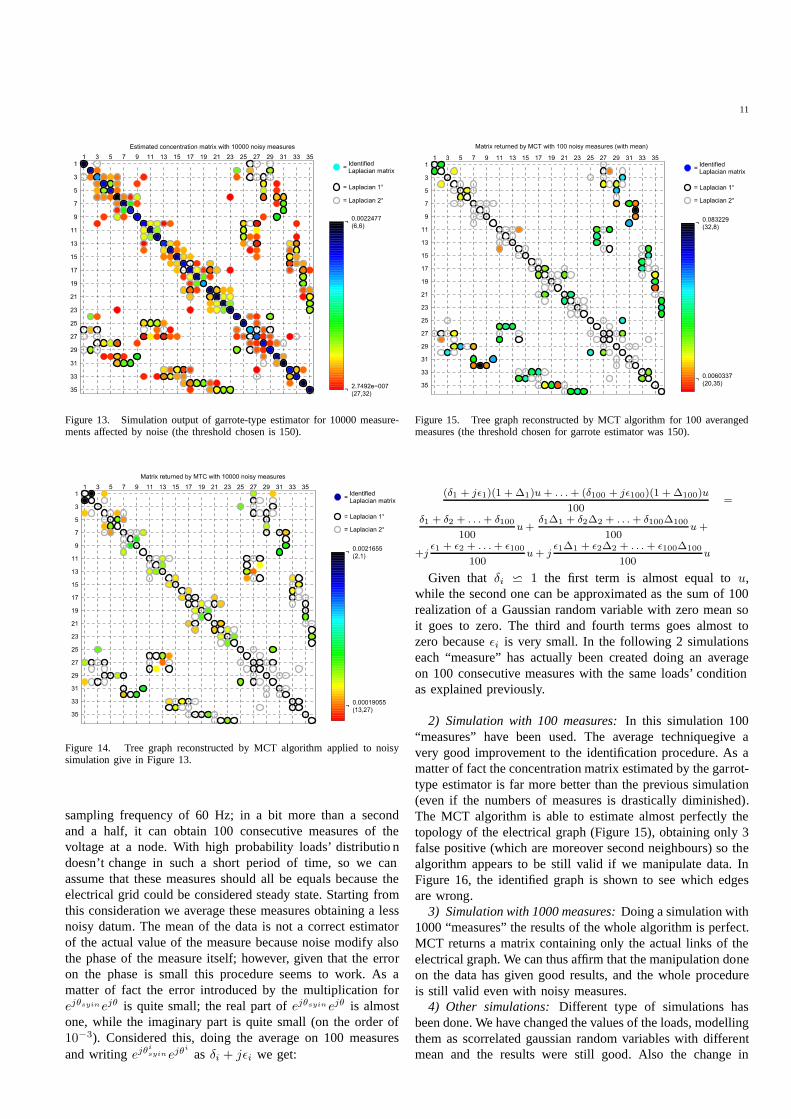
11

Figure 13. Simulation output of garrote-type estimator for 10000 measure-mentsaffected by noise (the threshold chosenis 150).

Figure 14. Tree graph reconstructed by MCT algorithm applied to noisysimulation give in Figure 13.

sampling frequency of 60 Hz; in a bit more than a secondand a half, it can obtain 100 consecutive measures of thevoltage at a node. With high probability loads’ distributiondoesn’t change in such a short period of time, so we canassumethat thesemeasures shouldall be equals becausetheelectrical grid could be considered steadystate.Startingfromthis consideration we averagethesemeasuresobtaining a lessnoisy datum. The meanof the datais not a correct estimatorof the actual valueof the measure becausenoisemodify alsothe phaseof the measure itself; however, given that the erroron the phaseis small this procedure seemsto work. As amatter of fact the error introducedby the multiplication forejθsyinejθ is quite small; the real part of ejθsyinejθ is almostone,while the imaginary part is quite small (on the order of10−3). Considered this, doing the averageon 100 measuresandwriting ejθ

isyinejθ

i

asδi + jǫi we get:

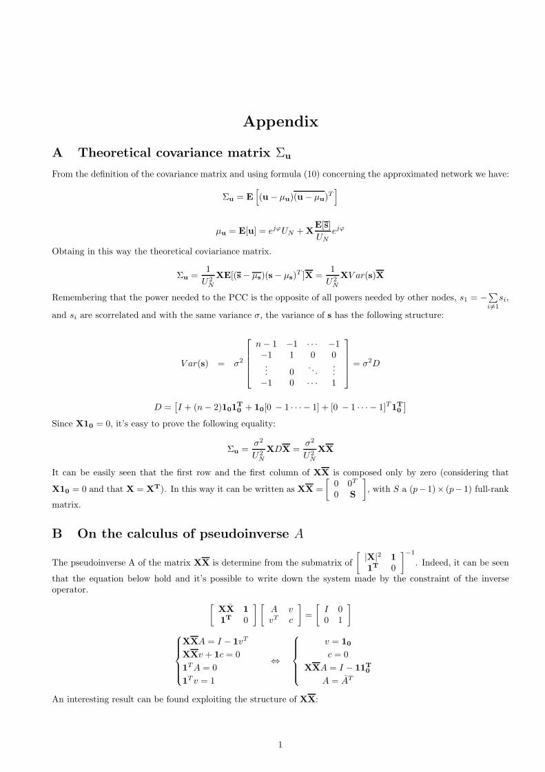
Figure 15. Treegraph reconstructed by MCT algorithm for 100 averangedmeasures (the thresholdchosenfor garrote estimator was150).

(δ1 + jǫ1)(1 + ∆1)u+ . . .+ (δ100 + jǫ100)(1 + ∆100)u

100=

δ1 + δ2 + . . .+ δ100

100u+

δ1∆1 + δ2∆2 + . . .+ δ100∆100

100u+

+jǫ1 + ǫ2 + . . .+ ǫ100

100u+ j

ǫ1∆1 + ǫ2∆2 + . . . + ǫ100∆100

100u

Given that δi ⋍ 1 the first term is almost equal to u,while the second onecanbe approximatedasthe sumof 100realization of a Gaussianrandom variable with zero meansoit goes to zero. The third and fourth terms goesalmost tozerobecause ǫi is very small. In the following 2 simulationseach“measure” has actually beencreated doing an averageon 100 consecutive measureswith the sameloads’conditionasexplainedpreviously.

2) Simulation with 100 measures: In this simulation 100“measures” have been used. The average techniquegive avery good improvement to the identification procedure. As amatterof fact theconcentration matrix estimated by thegarrot-type estimator is far more betterthanthe previous simulation(even if the numbers of measures is drastically diminished).The MCT algorithm is able to estimatealmostperfectly thetopology of the electrical graph (Figure 15), obtaining only 3falsepositive (which aremoreover second neighbours) so thealgorithm appears to be still valid if we manipulate data.InFigure 16, the identified graph is shown to seewhich edgesarewrong.

3) Simulation with 1000measures: Doingasimulation with1000“measures”the resultsof thewholealgorithm is perfect.MCT returns a matrix containing only the actual links of theelectrical graph.We canthusaffirm thatthemanipulationdoneon the datahasgiven good results,and the whole procedureis still valid even with noisy measures.

4) Other simulations: Different type of simulations hasbeendone. Wehavechangedthevaluesof theloads,modellingthem as scorrelatedgaussianrandom variables with differentmean and the results were still good. Also the change in

12

Figure 16. Topology identification corresponding tree graph obtain by MCTalgorithm of Figure 15.

valueof the impedencesof the line hasnot really affected theidentification. Concerning noises,it hasbeenobservedthat theaverageexpedient is not good if the phaseerror introducedby noise is quite higher than the one considered in theprevioussimulations,ascanbeexpected.So the identificationprocedure needs the misures to be not too noisy, and thisimplies that PMUs must introduce small errors (at least onthe phase).

VI . CONCLUSIONS AND FUTURE DEVELOPMENTS

This work shows the possibility to identify the topologyof an electric graph starting from measures taken by PMUsdevices arrangedin different places of the power grid. Thisresult hasbeenreached using a two-step-algorithm: first theconcentration matrix hasbeenestemated usinga garrote-typeestimator, and then the samematrix has beenelaborated toget the most likely treewich describes the electrical network(using MCT). The obtained results are satisfactory in theideal caseof noiselessmeasures, while the introduction oferrors in measures make the procedure unreliable. Howeverwith somereasonabledata-processingtheresultsarestill quitesatisfactory. Neverthlessdata-processingis possibleonly if thephaseerror is adequatelysmall.In practical casetheprocedurefound works only if PMUs give accuratemeasures.

Future developments can involve the distribution of thealgorithms in order to obtaina distributedalgorithm that runson each node. Another important feature to analyze is thepossibility of creating anautomaticprocedure to calculate thethresholdfor thegarrote-typeestimator. In theenda morepre-cisestudyon thevaluesof theconcentration matrix couldgiveimportant information about the network line impedences.

REFERENCES

[1] H. Sedghi and E. Jonckheere, “On the conditional mutual informa-tion in gaussian-markov structured grids,” Dept. of Electrical Engineer-ing,University of Southern California, Los Angeles.

[2] Y. L. Ming Yuan, “Model selection and estimation in the gaussiangraphical model,” 2007.

[3] S. Bolognani and S. Zampieri, “A distributed control strategy for reactivepower compensation in smartmicrogrids,” 2012.

[4] S. M. Francesco Bullo, Jorge Cortes, Distributed Control of RoboticNetworks. Princeton University Press,2009.

[5] S. L. Lauritzen, Graphical Models. Aalborg University: Clarendon Press- Oxford, 1996.

[6] L. C. Lau, “Bi partite roots of graphs,” 2004.[7] M. Fischietti, Lezioni di ricerca operativa. Edizioni libreria progetto

Padova, second ed.[8] W. H. Kersting, “Radial distribution testfeeders,” IEEE Power Engineer-

ing Society Winter Meeting.[9] A. Ben-Israel and T. N. Grevil le, Generalized Inverses: Theory and

Applications. RutgersCenter for OperationsResearch, RutgersUniversity,640 Bartholomew Rd, Piscataway, 2001.

Appendix

A Theoretical covariance matrix Σu

From the definition of the covariance matrix and using formula (10) concerning the approximated network we have:

Σu = E

[

(u− µu)(u− µu)T]

µu = E[u] = ejϕUN +XE[s]

UN

ejϕ

Obtaing in this way the theoretical coviariance matrix.

Σu =1

U2N

XE[(s− µs)(s − µs)T ]X =

1

U2N

XV ar(s)X

Remembering that the power needed to the PCC is the opposite of all powers needed by other nodes, s1 = −∑

i6=1

si,

and si are scorrelated and with the same variance σ, the variance of s has the following structure:

V ar(s) = σ2

n − 1 −1 · · · −1−1 1 0 0... 0

. . ....

−1 0 · · · 1

= σ2D

D =[

I + (n− 2)101T

0+ 10[0 − 1 · · · − 1] + [0 − 1 · · · − 1]T1T

0

]

Since X10 = 0, it’s easy to prove the following equality:

Σu =σ2

U2N

XDX =σ2

U2N

XX

It can be easily seen that the first row and the first column of XX is composed only by zero (considering that

X10 = 0 and that X = XT). In this way it can be written as XX =

[

0 0T

0 S

]

, with S a (p− 1)× (p− 1) full-rank

matrix.

B On the calculus of pseudoinverse A

The pseudoinverse A of the matrix XX is determine from the submatrix of

[

|X|2 1

1T 0

]−1

. Indeed, it can be seen

that the equation below hold and it’s possible to write down the system made by the constraint of the inverseoperator.

[

XX 1

1T 0

] [

A vvT c

]

=

[

I 00 1

]

XXA = I − 1vT

XXv + 1c = 0

1TA = 0

1T v = 1

⇔

v = 10

c = 0

XXA = I − 11T

0

A = AT

An interesting result can be found exploiting the structure of XX:

1

[

XX 1

1T 0

]

=

0 0T 1

0 S 1

1 1T 0

Changing the last and second rows and columns, it becomes

0 1 0T

1 0 1T

0 1 S

The inverse of this matrix leads to

∆ 1 α1 · · · αp−1

1 0 0 · · · 0α1 0...

... S−1

αp−1 0

, with αj = −

p−1∑

i=1

S−1(i, j) and ∆ =

p−1∑

i,j=1

S−1(i, j).

Finally, changing back the second and last rows and columns, the inverse of the given matrix is

∆ α1 · · · αp−1 1α1 0... S

−1...

αp−1

...1 0 · · · · · · 0

⇒ A =

∆ α1 · · · αp−1

α1

... S−1

αp−1

The pseudoinverse matrix of XXcan therefore be found deleting the row and column related with the PCC, invertingthe resulting matrix and reconstructing the elements of the PCC with easy calculations.

C Relationship between A and LL

Starting from equation (7), it’s possible to write down:

XL = I − 11T

0⇒ XXLL = XL−X11

T

0L ⇒ XXLL+X11

T

0L = I − 11

T

0(1)

XXA = XXLL+X11T

0L (2)

The given relationship is linear but matrix XX is singular, so pseudoinverses has to be used to solve the problem.The solution of a linear system like CXB = D, where the unknown matrix is X and C and B are singularmatrix, exists if and only if there are two matrices C(1) and B(1) such that CC(1)C = C, BB(1)B = B andCC(1)DB(1)B = D. C(1) and B(1) are a particular type of pseudoinverses (not unique). If the solution exists, thematrix which solves the system is

X = A(1)DB(1) + Y −A(1)AY BB(1)

where Y is an arbitrary matrix of appropriate dimension. For further details see [9]. From the properties of A followthat XXAXX = XX , so A is a possible pseudoinverse of XX that can be used in the solution of (2). Startingfrom (2), the existence of a solution with A as pseudoinverse can be proved in the following way:

XXA(XXLL+X11T

0 L) = XXAXXLL+XXAX11T

0 L

From the property of XX and A it’s easy to see that the first term in the sum equals XXLL. Using (1) and theproperty of A to analyze the second therm:

XXA−XXAXXLL−XXA11T

0=I − 11

T

0−XXLL = X11

T

0L

so

XXAXXLL+XXAX11T

0 L = XXLL+X11T

0 L.

The existence of a solution has thus been proved. The general solution is

2

A = AXXLL+ AX11T

0L+ Y −AXXY

with Y an arbitrary matrix of appropriate dimensions. Among all the possible choices for Y the null matrix isconsidered. Analyzing the first term,

AXXLL = (I − 11T

0)LL = LL

the solution can be written as:

A(I −X11T

0L) = LL (3)

Without any loss of generality, suppose that the node which is linked with the PCC is labelled as 2. In this way thefirst row of L has the following form: [ α −α 0 · · · 0 ], α 6= 0, since the sum of the elements of any row in Lhas to be 0. Moreover, remembering that the first row of X is made by zero entries, the sum of all the elements of

the first row is 0. Calling ai =p∑

j=1

X(i, j), it’s easy to prove that

(I −X11T

0 L) =

1 0 0 · · · 0αa2 1 + αa2 0 · · · 0αa3 −αa3...

... Ip−2

αap −αap

This matrix is invertible if and only if 1 + αa2 6= 0, that is α 6= −1/a2. This condition appears to be almost alwaysmet (at least in the simulation done for this work has always been met), so (3) can be solved using the inverse:

A = LL(I −X11T

0 L)−1

The inverse of the latter matrix has the following form:

(I −X11T

0 L)−1 =

1 0 0 · · · 0− αa2

1+αa2

11+αa2

0 · · · 0αa3+2α2a3a2

1+αa2

αa3

1+αa2

...... Ip−2

αap+2α2apa2

1+αa2

αap

1+αap

Due to the form of the inverse, A turns out to have the same element of LL except for the elements in position(1, 1), (1, 2), (2, 1), (2, 2).

D MaxDet and Nonnegative Garrote Estimator

We want to show the relation between the maxdet problem and the nonnegative Garrote estimator in order to applyYALMIP functions in the optimization of our semi-definite problem. Now, taking into account equation (12) and(13), we can see that

G(x) = C

=

d11c11 · · · d1nc1n...

. . ....

dn1cn1 · · · dnncnn

= d11

c11 · · · 0...

. . ....

0 · · · 0

+ dkh

0 · · · 0... ckh

...0 · · · 0

+ · · ·+ dnn

0 · · · 0...

. . ....

0 · · · cnn

and bTx = tr(CA) =[

c11a11 c12a12 . . . chkahk . . . cnnann]

·[

d11 d12 . . . dhk . . . dnn]T

. So, it

has been proven that C can be written as an affine function of dij , while tr(CΣu) can be written as a linear function

3

of dij , as needed by MaxDet problem formulation. Concerning the constraint∑

i6=j dij ≤ t dij ≥ 0 we can write asimilar relation as made for G(x):

F (x) = F0 + d11F11 + d12F12 + · · ·+ d1nF1n + · · ·+ dnnFnn

=

+t 0 . . . 0

0. . . 0

...... 0

. . ....

0 . . . . . . 0

+ d11

0 0 . . . 0

0 1 0...

... 0. . .

...0 . . . . . . 0

+ d12

−1 0 . . . 0

0. . . 0

...... 0 1

...0 . . . . . . 0

+ · · ·

= + d1n

−1 0 . . . 0

0. . . 0

...... 0 1

...0 . . . . . . 0

+ · · ·+ dnn

0 0 . . . 0

0. . . 0

...... 0

. . ....

0 . . . . . . 1

=

−∑

i6=j dij + t

+d11+d12

+d13. . .

+dnn

where Fij with i 6= j is the (n2+1)× (n2+1) matrix with -1 in position (1,1) and 1 in position (n(i−1)+j+1, n(i−1)+ j +1) , whereas if i = j the matrix Fij is made by the element 1 in position (n(i− 1) + j +1, n(i− 1) + j +1).Moreover, it’s easy to show that the constraint F (x) ≥ 0 gives:

F (x) ≥ 0 ⇐⇒ zTF (x)z ≥ 0 ∀z

zTF (x)z = z21(−d12 − · · · − d1n − · · · − dn,n−1 + t) + z22d11 + · · ·+ z2Ndnn

if zi = 0 for all i 6= 1 and z1 = 1, then

−∑

i6=j

dij + t ≥ 0

If zi = 0 for all i 6= 2 and z2 = 1, then

d11 ≥ 0

and so forth. Thus, the semi definite constraint F (x) ≥ 0 is equivalent to∑

i6=j dij ≤ t dij ≥ 0

E Numerical property of Laplacian element

E.1 Unweighted Laplacian

Theorem 1. First neighbours in an unweighted Laplacian Lu are negative, while second neighbours and the elements

on the diagonal are positive.

Proof. From the property of the Laplacian matrix the following statements are easy to prove:

Lu(i, i) = −∑

k 6=i

Lu(i, k)

Lu(i, j) < 0 ⇐⇒ (i, j) ∈ G

Considering now the element (i, j), i 6= j L2u and supposing that Lu(i, j) < 0, that is nodes i, j are firt neighbour:

4

L2u(i, j) =

n∑

k=1

Lu(i, k)Lu(k, j) =∑

k 6=i,j

Lu(i, k)Lu(k, j) + Lu(i, i)Lu(i, j) + Lu(i, j)Lu(j, j)

=∑

k 6=i,j

Lu(i, k)Lu(k, j)− Lu(i, j)∑

k 6=i

Lu(i, k)− Lu(i, j)∑

k 6=j

Lu(k, j)

Writing the summations explicitly:

L2u(i, j) = Lu(i, 1)Lu(1, j) + Lu(i, 2)Lu(2, j) + . . .+ Lu(i, n)Lu(n, j) +

+ Lu(i, j) [−Lu(i, 1)− Lu(i, 2)− . . .− Lu(i, j)− . . .− Lu(i, n)] +

+ Lu(i, j) [−Lu(j, 1)− Lu(j, 2)− . . .− Lu(i, j)− . . .− Lu(j, n)]

Writing first terms as Lu(i, k)Lu(k, j) =12Lu(i, k)Lu(k, j) +

12Lu(k, 1)Lu(k, j):

L2u(i, j) = Lu(i, 1)

[

1

2Lu(1, j)− Lu(i, j)

]

+ Lu(1, j)

[

1

2Lu(i, 1)− Lu(i, j)

]

+ Lu(i, 2)

[

1

2Lu(2, j)− Lu(i, j)

]

+ Lu(2, j)

[

1

2Lu(2, j)− Lu(i, j)

]

+ . . .+

+ Lu(i, n)

[

1

2Lu(n, j)− Lu(i, j)

]

+ Lu(n, j)

[

1

2Lu(n, j)− Lu(i, j)

]

− 2Lu(i, j)2

Since in Lu all the elements outside the diagonal are either 0 or −1, and L(i, j) = −1, all the terms between bracketsare positive ( 1

2L(k, h) − L(i, j) > 0 ). Finally the coefficient of each term in brackets is negative, so L2

u(i, j) isnegative. Concerning terms representing second neighbours in L2

u, they are positive because they can be writtenas:

L2u(i, j) =

n∑

k=1

Lu(i, k)Lu(k, j) =∑

k 6=i,j

Lu(i, k)Lu(k, j) + Lu(i, i)Lu(i, j) + Lu(i, j)Lu(j, j)

and Lu(i, j) = 0 since i and j are second negihbours; so

L2u(i, j) =

n∑

k=1

Lu(i, k)Lu(k, j) =∑

k 6=i,j

Lu(i, k)Lu(k, j)

which is a summation of positive (or null) terms. The diagonal elements in L2u are positive because they can be

written as norms.

E.2 Weighted Laplacian in Chain network structure

In a chain-structured electric network sign property is easy to verify even in the weighted Laplacian

Figure 1: Infinite chain-structured graph

The weighted Laplacian matrix associated to an electric network as the one in Figure 1 is like

L =

. . . −ǫ 0...

... . ..

−ǫ α+ ǫ −α 0 0 · · ·0 −α α+ β −β 0 · · ·· · · 0 −β β + γ −γ 0· · · 0 0 −γ γ + δ −δ

. .. ...

... 0 −δ. . .

5

with α = aα + jbα, aα > 0, bα < 0 (these considerations are valid for all the non-zero elements in the matrix).Calling F = LL, the demonstration looks at just one element wich represent a first neighbour in F, for example theelement in position (4, 3) :

F (4, 3) = −β(α+ β)− (β + γ)β = −(aβ − jbβ)(aα + jbα + aβ + jbβ)− (aβ − jbβ + aγ − jbγ)(aβ + jbβ)

Considering only the real part of F (4, 3):

−aβaα − 2a2β − bβbα − 2b2β − aγaβ − bγbβ < 0

The real part is then negative (the same proof holds for all the first neighbours in F ). The elements correspondingto second neighbours in F are in the second subidiagonal and in the second upperdiagonal (this is a consequence ofthe form of the Laplacian). To study the sign of the real part of second neighbours the element in position (5,3) isanalyzed:

F (5, 3) = (−γ)(−β) = (aγ − jbγ)(aβ + jbβ)

The real part of F (5, 3) is then:

aγaβ + bγbβ > 0

as stated.

E.3 Laplacian of generic Networks

In a generic electrical network, LL has positive real part elements on the diagonal and for the entries concerningsecond neighbours. Calling F = LL and cosidering that L = LT the diagonal elements are real and positive:

F (i, i) =

p∑

k=1

L(i, k)L(k, i) =

p∑

k=1

L(k, i)L(k, i) > 0.

Considering the entry in F for a second neighbour, for example F (i, j) with L(i, j) = 0:

F (i, j) =

p∑

k=1

L(i, k)L(k, j) =∑

k 6=i,j

L(i, k)L(k, j) + L(i, i)L(i, j) + L(i, j)L(j, j) =∑

k 6=i,j

L(i, k)L(k, j)

Considering the real part of a generic term of the summation, with L(i, k) = a + jb , a ≤ 0, b ≥ 0, L(k, j) =c+ jd , c ≤ 0, d ≥ 0

L(i, k)L(k, j) = ac+ bd ≥ 0

The real part of the summation is therefore positive.

F Signs of the weighted Laplacian

In this Appendix the dimonstration concernig sign in weighted Laplacian matrix is proven. The property is asfollow: considering L the real part of its non zero elements out of the diagonal is positive, and the imaginary partof the same is negative. Considering the impedence of any edge of the electric network, this has real and imaginarypart which are positive (the line is a passive element). Due to this fact its inverse has positive real part and negativeimaginary part. As a matter of fact

ze = ae + jbe, ae, be > 0 ⇒1

ze=

1

ae + jbe=

ae − jbea2e + b2e

.

A generic element of the weighted Laplacian can be computed as

L(i, j) =

p−1∑

k=1

A(k, i)1

zkA(k, j)

6

The incidence matrix A is such that only two elements per row are different from zero, a 1 and a -1. Exploitingthis fact, each term of the summation can be zero or − 1

zkand this proves the statement. This implies also that the

elements on the diagonal has positive real part and negative imaginary one (since the sum of the elements in a rowis 0).

7