Topology in Fractals

M. EUGENIA MONTIEL, ALBERT0 S. AGUADO and ED ZALUSKA

Electronics and Computer Science, University of Southampton, Highfield, Southampton SO17 lBJ, UK

(Accepted 13 November 1995)

Abstract-In this paper we consider the topological aspects of sets defined by fractal geometry. Topology, as a geometry, is extended to the definition of fractal structures by characterising equivalences in different levels of detail. A group of distinct topological fractals are defined by taking the equipotence and multiplicity properties of sets. Additionally, we define fractal metamorphosis as the sequence obtained by performing a continuous deformation of a fractal structure. In principle, this sequence would include elements of the same topological class. However, by extending the space where fractals are embedded, it is possible to perform a metamorphosis between two fractals belonging to different topological classes when defined in a plane. Copyright 0 1996 Elsevier Science Ltd

1. INTRODUCTION

Based on our perceptual experience of shapes, geometry provides a description of the way in which an object occupies a space. This description allows general principles applicable to geometrically equivalent objects to be established. Thus, geometry is used to characterise the world by means of recognising equivalent objects. This concept of geometry was first presented by Felix Klein [l, 21. Klein defined geometry as an abstraction process which forms a partition of mutually disjoint sets called equivalent classes and for which different principles are valid. Hence, the basic concept of geometry is equivalence and it represents a formalisation of the simple observation of analogies in the world. The definition of equivalence depends on how general or particular we want to develop a theory and different definitions have derived different geometries.

If objects are represented by sets then equivalence is characterised by a function or mapping. More formally, we define two sets X and Y as geometrically equivalent if there is a one-to-one mapping m,

m: X+ Y,

which leaves intact the geometrical properties of the sets.

(1)

Each geometry is associated to a group of mappings which are called groups of motions. Isometries (e.g., rotation, translation and reflection) are groups of motions which preserve distance between points and they characterise Euclidean geometry. In Euclidean geometry equivalence is referred to as congruence. When transformations of scale are included, the groups of motions are referred to as similarities. Other geometries such as affine, inversive, differential and topology are defined by more complex mappings based on more general properties [l, 21.

Topology can be considered the most general kind of geometry because its group of motions is defined by all the continuous invertible one-to-one mappings of the plane onto itself [3-51. A continuous invertible mapping in topology is denoted as a homeomorphism and the sets involved are homeomorphic to each other (topologically indistinguishable). In

this geometry a circle and a square, for example, are equivalent because they have the same continuity properties (closed curves without self-intersections).

Studies in topology have been concentrated on distinguishing homeomorphic objects by defining qualitative measures of those properties which remain intact when they are distorted by a homeomorphism. These properties are called topological invariants. Exam- ples of topological invariants include the number of intersections, number of holes, number of connected components in the set, compactness and Euler characteristic. These properties have been studied for two-dimensional curves and three-dimensional surfaces [5, 61. In this paper we use topological invariants to construct different types of fractals.

Fractal geometry was introduced by Mandelbrot [7] as a new geometry. If we follow the Klein definition of geometry we can see that there exists an important difference between fractal geometry and other geometries. While geometries are characterised by mappings which retain equivalences between two sets, fractal geometry represents the generalisation of equivalence to multiple scales within the same object.

By extending the notion of equivalence to multiple scales it is possible to recognise sets which are equivalent according to a particular geometry. The original formulation of fractal geometry was based on mappings defined by similarities. Afterwards, this definition was extended to include mappings of affine geometry [8]. In this paper we propose to consider topology as the geometry which defines equivalence. We distinguish types of fractals by considering different topological properties of the sets under construction (i.e. equipotent property of sets and multiplicities). Additionally, we define fractal metamorphosis as the sequence of sets obtained by performing a continuous deformation between fractals. The aim of this paper is to study the topology in fractal structures and to show how continuous transformations on these sets can be modelled. The importance of performing a deforma- tion of a recursive set is that it provides an extension of fractal descriptions to deformable forms.

This paper is organised as follows. In Section 2 we present a definition of recursive curves by using a functional equation. This definition provides a mathematical description where mappings can be represented by a trajectory in a parametric space. In Section 3 we consider invariant descriptors of fractal structures. These descriptors delineate topological classes. Section 4 contains some examples of homeomorphic mappings between fractals. We provide a deformation between two fractals belonging to different topological classes by extending the definition of mappings from the plane to the space. Finally, Section 5 presents conclusions.

2. COMPOSITION OF FBACTALS BY A FUNCTIONAL EQUATION

The main concern of topology has not been to derive geometric principles for particular classes of objects but to classify them based on whether the forms are equivalent according to homeomorphism. In this work we are interested in studying topological invariants which can be used for constructing fractal sets. In order to address this concept we represent fractals by using regular curves. This representation allows us to formulate topology on fractals as the application of topology of curves to multi-resolution descriptions.

A representation of fractal structures can be achieved by a recursive definition based on a functional equation [9]. In this section we propose a particular form of this definition and we relate it to the topology of curves. There exists a topological relationship between regular curves and fractals. Sierpinski showed in 1916 that it is possible to form an object which contains an image of all the curves in a topological sense. This universal represent- ation corresponds to a fractal set and it is called the Sierpinski carpet. Figure 1 shows the Sierpinski carpet and some examples of topologically equivalent objects (in columns) which

x Fig. 1. Sierpinski carpet and some examples of equivalent topological objects.

it includes. Notice that the carpet does not include any arbitrary curve but it contains a curve which is topologically equivalent. For example, we will never find a perfect circle but a square which is equivalent in a topological sense. For a discussion of the topological aspects of the objects embedded in the carpet the reader is referred to [lo]. The important feature of the carpet, for the present discussion, consists of the fact that a curve X can be seen as a subset of the fractal structure. That is,

X C F. (2) This means that a fractal can be composed of a union of curves,

F=Ux. (3) i

We consider the union in this equation as the linear (additive) combination of curves which describes different levels of detail. Consequently,

F = $ii’, for n --_, 01). (4) i=O

The curve Xi’, is represented through a periodic parametric polar function fi’. This function defines the locus of a curve as the end points of a vector in the complex plane and it corresponds to the Fourier expansion of a closed contour [ll-131.

fi’(0i) = CUikCOS(kWo8i) + biksin(kWoei), k

(5)

where the coefficients a& and bik repreSent two orthonormal vectors,

aik = axik + ja,, bik = bxi, + i&k.

(6)

In equation (5) the parameter W. will be set to unity and the range of values for the parameter ei will be [0, 27r). When the summation in k contains only one value, the points

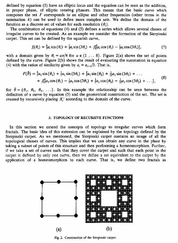
defined by equation (5) have an elliptic locus and the equation can be seen as the addition, in proper phase, of elliptic rotating phasors. This means that the basic curve which composes the set F corresponds to an ellipse and other frequencies (other terms in the summation k) can be used to define more complex sets. We define the domain of the function as a discrete set of values for each resolution (ei).

The combination of equations (4) and (5) defines a series which allows several classes of irregular curves to be created. As an example we consider the formation of the Sierpinski carpet. This set can be defined by the squarish curve,

fi’( Oi) = 4Ui sin (Oi) + $Ui sin (3Oi) + j[!jUi COS ( ei) - $Ui COS (30,)], (7)

with a domain given by Oi = uzr/4 for u E (1 . . . 8). Figure 2(a) shows the set of points defined by the curve. Figure 2(b) shows the result of evaluating the summation in equation (4) with the ratios of similarity given by Ui = Ui_i/3. That is,

F(8) = $2, sin (0,) + $2, sin (38,) + $2, sin (0,) + &a, sin (38,) + . . .

+ j[$21C0S(el) - $~~C0S(38~) + &0S(e,) - $~~CoS(38~) + . ..I. (8)

for rJ = (e,, e,, e,, . . .}. In this example the relationship can be seen between the definition of a curve by equation (5) and the geometrical construction of the set. The set is created by recursively placing Xi’ according to the domain of the curve.

3. TOPOLOGY OF RECURSIVE FUNCTIONS

In this section we extend the concepts of topology to irregular curves which form fractals. The basic idea of this extension can be explained by the topology defined by the Sierpinski carpet. As we mentioned, the Sierpinski carpet contains an image of all the topological classes of curves. This implies that we can obtain any curve in the plane by taking a subset of points of this structure and then performing a homeomorphism. Further, if we take a set of curves such that they cover the carpet and such that each point in the carpet is defined by only one curve, then we define a set equivalent to the carpet by the application of a homeomorphism to each curve. That is, we define two fractals as

Fig. 2. Construction of the Sierpinski carpet.

homeomorphic if we can perform a homeomorphism on the curves which compose each fractal. If we consider the set in equation (3) and we define another set G by,

G=Ux, (9)

for which Xi and yl are homeomorphic then we define F and G as homeomorphic. It is important to notice that although the Sierpinski carpet contains an image of all

curves to within topological equivalence it does not contain all the topological classes of fractals. This means that we cannot distort the points in the carpet by a continuous deformation to obtain any other fractal, and there must exist a group of sets which can be considered as a representative of different topological classes. One member of this group must include the Sierpinski carpet. Here, we define equivalent topological classes based on the equipotent property of sets and on multiplicities.

If we consider the composition of fractals presented in the previous section, then a fractal structure can be characterised by the topology of curves which form different levels of detail. This characterisation corresponds to the inclusion of the concepts of topological equivalence at multiple scales. That is, self-homeomorphic sets are defined by homeo- morphism within the same object. Then, the set F in equation (3) can be said to be self-homeomorphic if the curves fi’(0i) and J(Oj)Vi f j in equation (5) are homeomorphic. As, an example, suppose that we know that two sets F and G are self-homeomorphic and not-homeomorphic to each other, then we can define a not self-homeomorphic set by combining different levels of detail of both sets by,

H(e) = Chi(ei>,

I

if i is odd if i is even. (10)

Figure 3 shows the result of evaluating these curves for the particular definition of the sets given by,

A(ei) = Ufif+, 8i E {$, $7r, 2n}, &+,

gi(ei) = ag,dei, ei E {$r, $r, r, $r, $r, 2n}, ugi = +. (11)

Each level of detail within the sets F and G is topologically equivalent, whilst fi’(e,) and gi(8i) cannot be mapped to each other by a homeomorphism (see below). Consequently, the set iY defined by equation (10) is not self-homeomorphic.

Based on the topological characterisation of the composition of fractals it is possible to form equivalent classes. To avoid unnecessary complications, here we restrict ourselves to the definition of topological classes for self-homeomorphic objects. If F and G are considered as two fractals, then a transformation between both sets can be expressed as,

M: F(8) + G(e). (12)

If M is a continuous one-to-one mapping with an inverse (M-l), then F and G are homeomorphic. In the case when F and G are self-homeomorphic this relationship can be established by the nature of the mapping in one level of detail,

gi(W = Md(fh)). (13)

This definition is illustrated in the commutative diagram of mappings shown in Fig. 4. If

Fig. 3. Example of a not self-homeomorphic set.

fi+16> mi+r be gi+l

fi+2 6 mi+2 g i+2

Fig. 4. Diagram of maps between levels of detail of two sets.

fi’+r(Oi+r) = pi(fi’(8,)) and gi+r(Oi+r) = qi(gi(Oi)) then mi+r corresponds to the composite

mapping,

4+l = qpmpp;l. (14)

Accordingly, )?z~+~ will be a homeomorphism if mi, qi and pi are homeomorphisms. If mi is not a homeomorphism then mi+r will also not be a homeomorphism. Then if we determine the nature of Mi we can define the topological relationship between the sets F and G.

In order to delineate topological classes of fractals we will concentrate on studying when m, cannot be defined as a homeomorphism. The first topological invariance we will

(a) Sierpinski Gasket (ai= 3 ai-1) (b) Quadrilateral Gasket (a? jai-l)

(c) Pentagonal Gasket (ai= & ai-1) (d) Hexagonal Gasket (ai= 3 ai_1)

(e) Heptagonal Gasket (al= & a&I) (0 Octagonal Gasket (ai= ?j$ a,,)

Fig. 5. Examples of the fractal gasket family.

Fig. 6. Examples of a (a) homeomorphic and (b) not-homeomorphic mapping.

defines six points, it is not possible to define a homeomorphism between the points of both sets because the second curve has a multiplicity (intersection). That is, in order to perform a mapping we would have to relate the intersection point to two points on the circle. Thus, multiplicities constitute another topological invariant and we should only consider the classes defined by the gaskets containing more than one coefficient when there is not any multiplicity.

In order to characterise the set with multiplicities we can compute the number of times that a curve defines the same point. This number combined with the cardinality can be used to distinguish topological classes. Figure 7 shows an example of the definition of two fractal sets based on cardinality 6 and one multiplicity. The set in Fig. 7(a) defines the multiplicity twice whilst the set in Fig. 7(b) defines the multiplicity three times. It is clear that if the number of times that the curve defines the multiplicity differs then we cannot pair off the elements of both sets and the fractals are not-homeomorphic. Notice that we choose discrete points at each multiplicity when these occur.

A complete set of multiplicities can be characterised by adding all the values which define a point. That is, for the point defined by 0, the number of multiplicities is,

L, = 2 C(e,, Oi), VeisD

for C(O,, 0,) i

{

~~~~er~ f(ei). (18)

Two curves will be topologically equivalent only if they have the same characteristic values L,. Thus, we can establish that two fractals belong to different topological classes when the number of multiplicities differs and this definition together with cardinality provides quantitative topological invariants for fractal sets.

(a) 09

Fig. 7. Examples of definition of fractals with (a) dual (lemniscate) and (b) tetra (rose of three petals) multiplicity.

4. TOPOLOGIC MAPPINGS ON FRACTALS: FRACTAL METAMORPHOSIS

In this section we shall consider mappings between two recursive structures. These mappings are defined by a curve dependent on time. We define fractal metamorphosis as the sequence obtained by performing a continuous deformation of a fractal structure.

The mapping A4 in equation (12) can be parameterised in order to provide a time-dependent description of a shape. The parameterisation can be formalised by redefining A4 as,

M: F(8) x Z + G(8), (19)

where Z = [0, l] such that M(8, 0) = F(8) and M(8, 1) = G(8). The family of sets obtained from the sequence M(8, t) constitutes a fractal metamorphosis.

Based on the definition of fractals in equation (4) we characterise the mapping in equation (19) by several mappings at different levels of detail. That is, a dynamic transformation is obtained by parameterising Mi in equation (13) as,

mi(Oi, ?>

for mi(ei, 0) = j(ei), mi(ei9 1) = gi(ei)9 (20)

and where the complete transformation M is defined by mi(Bi, t) for all i. The parameterisation in this equation corresponds to a curve which defines how fi’(@) will be deformed until it occupies the space defined by gi( f3i). In general M can be defined to generate a myriad of topologically equivalent objects which could describe a dynamic

behaviour. Here, we will formulate the transformation between fractals by a linear mapping of the form,

mi(ei, t, = (l - r)fi’(ei) + tgi(ei) for t 6 [0, 11. (21)

As an example we can consider a mapping between the octagonal gasket and the Sierpinski carpet. These two sets are homeomorphic and the mapping which makes them equal consists of deforming the circle which defines the gasket into a squarish shape which defines the carpet. This deformation can be performed by combining equation (7) and one resolution of equation (15) as,

mi(8i, t) = (1 - t)u,sin(ei) + t($Z,sin(eJ + &,sin(3ei)) + i[(l - t)u~COS(fl,)

+ &, COS (@) - $zgi COS (3 @))I,

for ex = $ii~f_,, ag, = fu,,_,. (22)

The definition of IZ resolutions can be expressed by (see equation (17)),

M(8, t) = i ERZi(@i, t), for ei = u$r. (23) i=l u=l

The fractal metamorphosis defined for this curve is shown in Fig. 8. In the sequence the trajectory that follows each point corresponds to a discretisation (by the variable t) of a linear mapping which defines both sets as topologically equivalent.

Because a metamorphosis is defined by decomposing a homeomorphism, in principle it can only represent a sequence which produces a transformation between two fractals belonging to the same topological class. Nevertheless, by extending the space where fractals are embedded by one dimension it is possible to change their topological character. Transformations between curves belonging to two different topological classes can be performed if we consider that they are embedded in a three-dimensional space and that a fractal is the resulting projection of the curves into a plane. Therefore, multiplicities can be addressed as different points and mappings between classes can be defined.

The formation of sets by projections of three-dimensional curves is exemplified in Fig. 9 where a lemniscate is formed by twisting a circle in a three-dimensional space. Here, although the projection of the circle and the lemniscate results in two sets belonging to two different topological classes, it is possible to define a three-dimensional one-to-one

Fig. 8. Metamorphosis between the octagonal gasket and the Sierpinski carpet.

Fig. 9. Three-dimensional definition of a circle and a lemniscate.

mapping which makes both sets equivalent. That is, it is possible to align the points of two three-dimensional homeomorphic sets in such a way that a projection on a plane corresponds to two not-homeomorphic two-dimensional sets.

In general, the definition of a three-dimensional mapping which performs a specific two-dimensional metamorphosis between two not-homeomorphic sets, leads to a compli- cated formulation. Because we defined fractals by a parameterised expression, this mapping can be obtained based on the equations which define their projections. That is, the parameterisation of equation (5) distinguishes different points in the plane by different values of the variable 8, thus the points corresponding to multiplicities can be addressed separately in order to be mapped into different points. This concept is illustrated in the next example where the metamorphosis between fractals defined by a circle and a lemniscate resembles a folding in a three-dimensional space which reveals the true nature of the transformation.

In order to obtain a linear time parameterisation between the hexagonal gasket and a fractal with one multiplicity, we formulate the mapping between a circle and a lemniscate

by,

rni(& t) = U&(1 - t) cos (0i) + agif sin (6;) + i[uh(l - t) sin ( ei) + a$ sin (2e,)],

for ah = &_, , ug, = &,i_1. (24)

The definition of this mapping for the complete set corresponds to equation (23) with the limit of the summation on u up to 6 and 8i = urr$. Figure 10 shows different stages of the metamorphosis obtained for eight values of t. Note how, in the last stage, two points in each resolution which form the hexagonal gasket are aligned in space such that the projection on the plane produces one multiplicity which defines the lemniscate.

The idea of projecting a curve in a space into a plane, can be used to obtain deformations of curves. By careful choice of the discretisation, this can provide a metamorphosis between two non-equipotent sets. This metamorphosis between non- equipotent sets can be simply defined by a change in frequency. This is achieved by rewriting equation (23) as,

M(O, t) = i it?Zi(Bi, t), i=l u=l

Fig. 10. Metamorphosis between the hexagonal gasket and a fractal defined by a curve with one multiplicity.

for T1 the period which defines F and T2 the period which defines G. In this equation the limit w corresponds to the number of points which define the fractal and the change of T(t) from T, to T2 produces a change in the frequency which unfolds the multiplicities.

Based on equation (25) we can, for example, obtain a metamorphosis between the Sierpinski gasket and the hexagonal gasket. By considering definition (17) and afi and agi the coefficient of each gasket, respectively,

M(8, t) = i &(I - t)afi + tagi)eiUT(‘). (26) i=l u=l

Figure 11 shows the evaluation of this expression for a linear definition of T given by,

T(t) = (1 - O&T) + &). (27)

Because the limit of the index u is constant then all the sets in the sequence have the same cardinality. This means that each resolution of the Sierpinski gasket contains three multiplicities which are unfolded to generate the six points of the hexagonal gasket.

Fig. 11. Metamorphosis between the Sierpinski gasket and the hexagonal gasket.

Notice that although we have considered transformations in the curve which defines the sets and in the number of multiplicities separately, it is possible to combine them into just one transformation. This is the case for the metamorphosis shown in Fig. 12 which transforms the Sierpinski gasket into the Sierpinski carpet. In this example there exists a change of cardinality from 3 to 8 points and the curve changes from a circle to a square. By combining equations (23) and (25) the metamorphosis is defined by the mapping,

+ iSin(3OJ ] * [( ‘) - icos(3ei)]9 + ]U;(t) 1 + 5 COS(Bi)

with Bi = UT(~)

for T(t) = $rr(r - 1) + $rTt,

Ui(t) = Ui-I(?)(; - :I+)* (28)

In general, by combining changes in the form and in the number of multiplicities it is possible to perform some metamorphoses between recursive sets. The sequence in a metamorphosis characterises dynamics as a deformation of the scaled definitions of a fractal. In the previous examples we restrict ourselves to the same transformation in each scale, nevertheless, this only represents the simplest definition of a transformation and more complex mappings can include different transformations between resolutions.

As the last part of this section we shall consider mappings which define a new level of detail by performing a deformation of the previous resolution of a set,

4i: gi(4) + gi+1(f%+A. (2%

According to the diagram of maps shown in Fig. 4 this mapping can be seen as the resulting deformation between two sets F and G,

qi = ~i+~‘pi”~7’. (30)

That is, qi corresponds to a composite mapping which includes the definition of an original set pi as well as a deformation M. If M is parameterised in time by equation (19) then a

Fig. 12. Metamorphosis between the Sierpinski gasket and the Sierpinski carpet.

metamorphosis obtained by a continuous deformation of a fractal structure can be redefined by the homotopy,

40;, t) = f?Zi+r(pio??l;‘(ei, t), t). (31)

This mapping specifies a deformation in time of the curves which form a recursive structure and it can be completely defined through only two types of transformations which correspond to a change in scale and rotation of the vectors a& and bik which characterise the sinusoid in equation (5). That is,

4i(@9 f) --j aik(t), bik(t)a (32)

By rewriting equation (5) in a phase-magnitude form, the modulus and angle of these vectors can be directly used to specify the evolution in time of a set,

gi(ei, t) = Claik(t)leiPa”‘cos(ei) + Ibik(t)Ie”Pa”““‘2’sin(8i), (33) k

where Pik(t) iS the angle Of a&* The term 9r/2 ensures that the vectors aik and bik are orthogonal. Notice that a change of phase and amplitude not only defines a change of rotation and scale between which define the structure. (33) can be rewritten as,

levels of resolution but it includes deformations in the curves When aik(f) and bik(f) have the same modulus then equation

gi(ei, t) = &&)ld(ei+P~(‘)). k

(34)

We have already mentioned that a change in amplitude modifies the size of the sub-parts which form a structure and when the amplitude in all the levels of detail is reduced, the resulting fractal is formed by dust clusters. In the previous examples we used an amplitude ratio which defines a geometric shape which fits inside the previous resolution. When the ratio is greater than this value, lower resolutions are overlapped producing a textured image. Figure 13 shows a textured set generated by using the definition of the Sierpinski triangle (equation (17)) with an amplitude reduction rate defined by Ui = 3Ui_1/2. In this example different colours were assigned based on the values of ei. Substructures with the same colour were created when 8, = 0 and ej # 0 Vi > i. Other representations of texture could include the approach of Barnsley [15] which assigns values to the points in the space according to the frequency with which they are defined.

The patterns generated by a change in the coefficients which define equation (34) are more visually attractive when they include a change in phase (Pik(f)). The sequence shown in Fig. 13 was obtained by defining Pik(t) in equation (34) as a change proportional to time. This transformation constitutes the simplest deformation obtained by a change of phase and does not involve a change in the shape of the curves which define the structure, nevertheless, it produces a set which follows a chaotic movement where one cannot predict the path of a point in the space.

The metamorphosis shown in Fig. 14 includes both a change in amplitude and phase of a fractal defined by a branching structure. The modelling of the dynamics of these kinds of structures has been previously considered [16]. The set in the figure was created by joining with lines the points in consecutive levels of resolution. Each resolution is obtained by rewriting the description of the spleenwort fern [lo] in terms of equation (34) as,

gi(ei) = ui ,$%+P,),

with pi = ei_r + pi-1 + ycos($+_i(ei_i) + @ii(e Ui = r(Oi)Ui_l,

for k(ei) E (0, R), 6 E {-+I?, 0, &I.

(35)

Fig. 14. Example of a deformation with change of amplitude and phase.

This equation defines a positive or negative rotation of y radians depending on the two possible values of @. In order to generate the branching structure the rotation is defined by preserving the orientation of the previous resolution.

The fern shown in Fig. 14 is composed of three transformations. The rotation is defined by a small value of y (y = 0.1) and the r and C#J values are given by,

ei r(ei) -5/l&r 0.3

#i(,ei)

0 0.8 0 5/1&T 0.3 ?r

The branch drawn when 8i = 0 forms an axis of symmetry and it is bent by the value of y, The other definitions of 8 result in two symmetric limbs which are bent toward the axis of symmetry. By using quadratic polynomials to obtain the values of @ and r shown in the previous table and by extending equation (35) to n resolutions the complete definition of the fern is,

for Ui = constant, ai = Ui_i(ei_i)(0.8 - 1.44ei),

C&-J = 0, ai = 6 + YCOS(&-,(ei-1) + Mei)),

4l = 0, $i(ei) = 1.8ei + 2.0703.

(36)

The change in amplitude which defines the metamorphosis consists of a linear variation which produces an infinitely-small structure at the beginning. That is,

Ui(Bi, t) = Ui_i(8i_r, t)(0.8 - 1.448,)(1 - t). (37)

The phase change is defined by an inverse of a sine function. This increases the rotation frequency of each resolution and because we want the movement to be in one direction for any value of ei it is added to the angle. That is,

G(g) = i,,Ce,, t)8(~i-'(ei-')+~i(B',,+i~in(f). (38) i=l

Notice that the rotation is defined by sin(r’8,) and the inverse provides the angle for the frequency i for the evolution in time (t).

As a last example of a geometric mapping we shall consider the simple metamorphosis of a non-deterministic set. This set is defined by equation (34) with a stochastically increasing ratio between resolutions and a stochastic rotation,

ai = NORMAL(ai_i(t)*2, o,(t)),

pi(t) = Pi-i(t) + NORMAL@(t), op)* (39)

Here NORMAL corresponds to a function which returns a number with a normal probability distribution with mean and variance given by the first and second arguments, respectively. Because the amplitude is increased, the resulting structure has the appearance of dust. The objective of this metamorphosis is to obtain a sequence which reduces the variation of a set of points (i.e., to make them appear more ordered) by performing a circular movement. This is achieved by reducing the values of a(t) and p(t) proportional to time. Figure 15 shows a metamorphosis defined by this mapping. During the sequence the farthest points from the centre rotate faster simulating a tidal force.

5. CONCLUSION

In this paper we have considered recursive structures based on the geometry topology. With this approach to fractal geometry we studied a concept of

defined by topological

_ . equivalence for fractal sets. This concept is relevant for the analysis and synthesis of models which attempt to explain the continuous distortion of forms represented by fractal geometry. In the analysis of shapes it is useful to have descriptors which remain unchanged by continuous distortions. In order to provide these descriptors we have considered two topological invariants characterised by cardinality and multiplicities.

We have created a transition between two fractals by parameterising a continuous mapping in time. Then we have shown that these mappings can be completely specified by a change in amplitude and phase of the coefficients which define a structure. Future work will focus on the extension of the concepts developed in this paper to structures defined in three-dimensional space as well as the study of how geometric mappings can provide rules of articulation to define the relevant geometry for dynamic aspects of a structure.

Acknowledgements-The authors would like to thank Dr D. Chillingworth from the Department of Mathematics for his useful comments and discussion. M. E. Montiel and A. S. Aguado are grateful to the CONACyT (Consejo National de Ciencia y Tecnolgia, Mexico) and to the DGAPA (Direcci6n General de Asuntos de1 Personal Academico) from the UNAM (Universidad National Autbnoma de Mexico) for their financial support.

REFERENCES

1. E. A. Lord and C. B. Wilson, The Mathematical Description of Shape and Form, Series Mathematics and its Applications. Ellis Horwood, Chichester, UK (1986).

2. M. J. Greenberg, Euclidean and Non-Euclidean Geometries: Development and History. W. H. Freeman, New York, USA (1994).

3. B. Mendelson, Introduction to Topology. Black & Son Limited, Glasgow, UK (1963). 4. J. Dugundji, Topofogy. Allyn & Bacon Inc., Boston, USA (1966). 5. M. Nakahara, Geometry, Topology and Physics, Graduate Student Series in Physics. Adam Hilger, IOP

Publishing Ltd., Bristol, England (1990). 6. C. Lee, T. Poston and A. Rosenfeld, Holes and genus of 2D and 3D digital images, CVGIP: Graphical

ModeLF and Image Understanding 55(l), 20-47 (1993). 7. B. B. Mandelbrot, The Fractal Geometry of Nature, W. H. Freeman, San Francisco, USA (1982). 8. B. B. Mandelbrot, Fractal geometry: what is it, and what does it do?, in Fractals in the Natural Sciences: A

Discrcssion, organized and edited by M. Fteishmann, F. J. Tilde&y and R. C. Bail. Princeton University Press, UK (1990).

9. S. Dubuc, Models of irregular curves, in Fractals: Non-integral Dimensions and Applications. John Wiley & Sons, Chichester, UK (1991).

10. H.-O. Peitgen, H. Jurgens and D. Saupe, Chaos and Fractals: New Frontiers of Science. Springer, New York, USA (1992).

11. F. P. Kuhl and C. R. Giardina, Elliptic Fourier features of a closed contour, Computer Graphics and Image Processing 18, 236-258 (1982).

12. P. J. van Otterlo, A Contour-oriented Approach to Shape Analysis. Prentice-Hall International, UK (1991). 13. C. T. Zahn and R. Z. Roskies, Fourier descriptors for plane closed curves, IEEE Transactions on Computers

21(3), 269-281 (1972). 14. H. Jones, Fractals before Mandelbrot: A selective history, in Fractals and Chaos, pp. 15-25, Springer,

New York, USA (1991). 15. M. F. Barnsley, A. Jacquin, F. Malassenet, L. Reuter and A. D. Sloan, Harnessing chaos for image synthesis,

Computer Graphics Proceedings, SIGGRAPH’88 22(4), 131-140 (1988). 16. T. Pijschel and H. Malchow, A simple model for growth of ramified leaf structures, Chaos, Solitons &

Fractafs 4(10), 1883-1888 (1994).