Topology Optimization of Turbine

Manifold in the Rocket Engine

Demonstrator Prometheus

Filip Jensen

Space Engineering, master's level

2018

Luleå University of Technology

Department of Computer Science, Electrical and Space Engineering

Topology Optimization of Turbine Manifold in theRocket Engine Demonstrator Prometheus

Filip Jensen

© Filip Jensen, 2018.

Supervisor: Marcus Johansson, GKN Aerospace Sweden ABExaminer: Peter Jeppsson, Department of Engineering Sciences and Mathematics

Master’s Thesis 2018Department of Computer Science Electrical and Space EngineeringSpace Engineering - Spacecraft and InstrumentationLuleå University of TechnologySE-971 84 LuleåTelephone +46 920 49 10 00

Luleå, Sweden 2018

i

Topology Optimization of Turbine Manifold in theRocket Engine Demonstrator Prometheus

Filip JensenDepartment of Computer Science, Electrical and Space EngineeringLuleå University of Technology

Abstract"The art of structure is where to put the holes"Robert Le Ricolais, 1894-1977

The advantages of Topology Optimization (TO) are realized to a large extent due tothe manufacturing freedom that Additive Manufacturing (AM) offer, compared tomore conventional manufacturing methods. AM has the advantage of manufactur-ing shallow and complex structures previously not possible, and consequently opensup a whole new design spectrum.

This thesis investigates the possibilities of using Topology Optimization as a tool tofind stronger and lighter designs for the inlet turbine manifold in the rocket enginedemonstrator Prometheus. The manifold is optimized by giving it more mass, sub-jecting it to load cases and pushing the topology optimization to make the manifoldmeet the weight requirement without exceeding the yield strength. Result validationindicates that the pressure and thermal loadings are the most prominent.

The current topology optimization tools in ANSYS do not support optimizationdue to thermal features and thus optimization in the presented work has only beenable to consider static structural loads. Nevertheless, it is possible to optimize themanifold due to static structural loads and achieve a manifold which satisfies theweight requirement. However, optimization tools due to thermal loading would bea desirable feature in the future.

Keywords: Additive Manufacturing, Prometheus, Rocket Engine, Topology Opti-mization.

ii

AcknowledgementsI would like to thank Rikard Nedar and the department of Rotors at GKN Aerospacein Trollhättan for giving me this opportunity - especially Marcus Johansson for thesupport and supervising throughout this thesis. Thank you Gunnar Högström forbeing enthusiastic and helping me with various difficulties related to structural anal-yses and meshing. Thank you Håkan Gullmander for the support in creating modelsas well as providing me with models.

I am very glad for my participation in the Prometheus project and would like tothank everyone involved in the project group at GKN. Thank you Peter Jeppssonfor being a helpful and supportive examiner and teacher. Thank you Jonas Karlssonat the IT department of GKN Aerospace for always helping me with technicalities.

Filip Jensen, Trollhättan, June 2018

iv

Acronyms DescriptionAGS Ariane Group SAAM Additive ManufacturingCAA Computer Aided AnalysisCAD Computer Aided DesignCAE Computer Aided EngineeringCAM Computer Aided ManufacturingDOF Degree of FreedomFE Finite ElementGUI Graphical User InterfaceGKN Guest, Keen & NettlefoldsLCH4 Liquid MethaneLOX Liquid OxygenLPB Laser Powder BedMMA Method of Moving AsymptotesRSM Remote Solver ManagerSIMP Solid Isotropic Microstructure with PenalizationSTL StereolithographyTO Topology OptimizationTOM Turbine Outlet Manifold

Symbols Description Unit (metric)Ead Admissable stiffness tensor [Pa]E0ijkl Stiffness tensor of material [Pa]

f Load vector [N]t Boundary traction [-]Γτ Traction part [-]u Displacement [m]v Displacement [m]Ω Reference domain [m3]dΩ Material boundary [m3]Ωmat Occupying part [-]Ke Element stiffness matrix [Pa]K Global stiffness matrix [Pa]l Load linear form [-]ρ Relative/pseudo density [-]ρj Density of an element [kg/m3]ρ0 Density of the material [kg/m3]ε Strain tensor [Pa]

vi

viii

Contents

List of Figures xi

List of Tables xiii

1 Introduction 11.1 Prometheus . . . . . . . . . . . . . . . . . . . . . . . . . . . . . . . . 11.2 Aim . . . . . . . . . . . . . . . . . . . . . . . . . . . . . . . . . . . . 2

2 Background study 32.1 Topology Optimization . . . . . . . . . . . . . . . . . . . . . . . . . . 3

2.1.1 Theory of Topology Optimization . . . . . . . . . . . . . . . . 42.1.1.1 Structural Optimization - Minimum Compliance . . . 42.1.1.2 SIMP: Solid Isotropic Material with Penalization . . 62.1.1.3 Filters and sensitivity . . . . . . . . . . . . . . . . . 7

2.1.2 Topology Optimization Solvers in ANSYS . . . . . . . . . . . 82.1.2.1 Sequential Convex Programming . . . . . . . . . . . 82.1.2.2 Optimality Criteria . . . . . . . . . . . . . . . . . . . 8

2.2 Additive Manufacturing . . . . . . . . . . . . . . . . . . . . . . . . . 82.2.1 Method of printing . . . . . . . . . . . . . . . . . . . . . . . . 10

2.2.1.1 EOS M 400- 3D Printing of Metal Parts on an In-dustrial Scale . . . . . . . . . . . . . . . . . . . . . . 10

3 Software Description 133.1 ANSYS . . . . . . . . . . . . . . . . . . . . . . . . . . . . . . . . . . 13

3.1.1 Workbench 19.0 . . . . . . . . . . . . . . . . . . . . . . . . . . 133.1.1.1 Mechanical . . . . . . . . . . . . . . . . . . . . . . . 133.1.1.2 SpaceClaim Direct Modeler . . . . . . . . . . . . . . 13

3.2 Siemens NX . . . . . . . . . . . . . . . . . . . . . . . . . . . . . . . . 143.3 Altair Engineering . . . . . . . . . . . . . . . . . . . . . . . . . . . . 14

3.3.1 HyperWorks . . . . . . . . . . . . . . . . . . . . . . . . . . . . 143.3.1.1 HyperMesh . . . . . . . . . . . . . . . . . . . . . . . 143.3.1.2 OptiStruct . . . . . . . . . . . . . . . . . . . . . . . 143.3.1.3 HyperView . . . . . . . . . . . . . . . . . . . . . . . 14

4 Methods 154.1 Material . . . . . . . . . . . . . . . . . . . . . . . . . . . . . . . . . . 164.2 Geometry . . . . . . . . . . . . . . . . . . . . . . . . . . . . . . . . . 16

ix

Contents

4.2.1 Analysis and Topology Optimization . . . . . . . . . . . . . . 174.3 Analysis setup . . . . . . . . . . . . . . . . . . . . . . . . . . . . . . . 17

4.3.1 Preparing the Topology Optimization Analysis . . . . . . . . . 184.3.2 Boundary Conditions and Loads . . . . . . . . . . . . . . . . . 194.3.3 Topology Optimization parameters and constraints . . . . . . 20

4.3.3.1 Analysis settings . . . . . . . . . . . . . . . . . . . . 204.3.3.2 Optimization Region . . . . . . . . . . . . . . . . . . 204.3.3.3 Objective . . . . . . . . . . . . . . . . . . . . . . . . 214.3.3.4 Response Constraints . . . . . . . . . . . . . . . . . 214.3.3.5 Manufacturing Constraints . . . . . . . . . . . . . . 21

4.4 Limitations and Difficulties . . . . . . . . . . . . . . . . . . . . . . . . 224.4.1 Finite Element Solution work flow . . . . . . . . . . . . . . . . 234.4.2 Post-processing and design validation . . . . . . . . . . . . . . 24

4.5 2D Study . . . . . . . . . . . . . . . . . . . . . . . . . . . . . . . . . 244.5.1 Load cases . . . . . . . . . . . . . . . . . . . . . . . . . . . . . 254.5.2 Design approach . . . . . . . . . . . . . . . . . . . . . . . . . 254.5.3 Casing . . . . . . . . . . . . . . . . . . . . . . . . . . . . . . . 25

4.6 Capable Diaphragm . . . . . . . . . . . . . . . . . . . . . . . . . . . . 264.6.1 Four Case Study . . . . . . . . . . . . . . . . . . . . . . . . . 27

4.7 3D Study . . . . . . . . . . . . . . . . . . . . . . . . . . . . . . . . . 284.7.1 Design approach . . . . . . . . . . . . . . . . . . . . . . . . . 294.7.2 Loads . . . . . . . . . . . . . . . . . . . . . . . . . . . . . . . 30

5 Results 335.1 2D . . . . . . . . . . . . . . . . . . . . . . . . . . . . . . . . . . . . . 33

5.1.1 Casing Designs . . . . . . . . . . . . . . . . . . . . . . . . . . 335.1.2 Four Case Study - Comparing Diaphragm and Torus . . . . . 37

5.1.2.1 Case 1 - Original Diaphragm and Original Torus . . 375.1.2.2 Case 2 - Original Diaphragm and Optimized Torus . 385.1.2.3 Case 3 - Optimized Diaphragm and Original Torus . 415.1.2.4 Case 4 - Optimized Diaphragm and Optimized Torus 445.1.2.5 Case 4 - Extended Work . . . . . . . . . . . . . . . . 45

5.2 3D . . . . . . . . . . . . . . . . . . . . . . . . . . . . . . . . . . . . . 465.2.1 Inlet Optimization . . . . . . . . . . . . . . . . . . . . . . . . 475.2.2 Fully Enclosed Manifold . . . . . . . . . . . . . . . . . . . . . 50

6 Conclusion 55

7 Further Work 57

Bibliography 59

A Appendix TOM I

x

List of Figures

1.1 Conceptual illustration of the Prometheus rocket engine - courtesy ofAriane Group Holding, [23] . . . . . . . . . . . . . . . . . . . . . . . . 2

2.1 Example of Michell tension-compression 2D truss case. . . . . . . . . 32.2 Three different structural optimization types. a) Size; b) Shape; c)

Topology. (figure 1 in [1], courtesy of M.P Bendsoe & Ole Sigmund) . 42.3 Checkerboard problem for cantilever beam. a) Initial design, b) so-

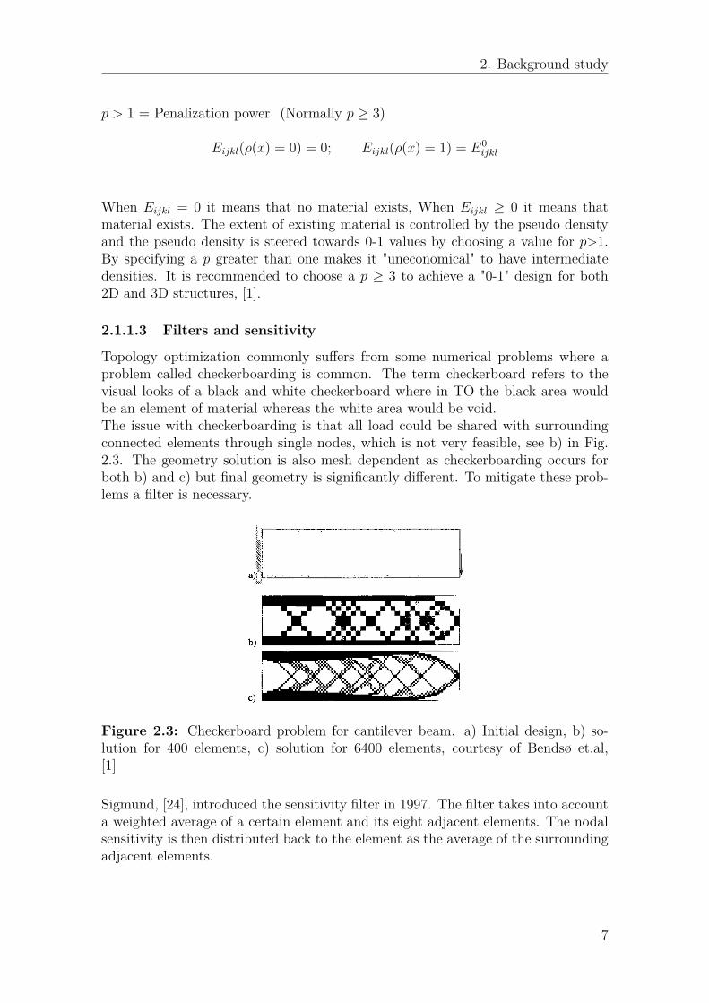
lution for 400 elements, c) solution for 6400 elements, courtesy ofBendsø et.al, [1] . . . . . . . . . . . . . . . . . . . . . . . . . . . . . . 7

2.4 Fully supported element in 2D.Courtesy of Matthijs Langelaar, [15] . 92.5 Laser Powder Bed manufacturing illustration, (from [8] courtesy of

C. Dordlofva . . . . . . . . . . . . . . . . . . . . . . . . . . . . . . . . 102.6 EOS M 400 DMLS . . . . . . . . . . . . . . . . . . . . . . . . . . . . 11

4.1 Turbine manifold geometries in 2D and 3D . . . . . . . . . . . . . . . 174.2 ANSYS Workbench typical setup . . . . . . . . . . . . . . . . . . . . 174.3 Preprocessing example in SpaceClaim of geometry for a certain 2D case 184.4 Manifold in 2D and 3D with relevant loads . . . . . . . . . . . . . . . 194.5 The general work flow scheme of Topology Optimization, courtesy of

Shun Wang [7] . . . . . . . . . . . . . . . . . . . . . . . . . . . . . . . 234.6 Example of manifold with added geometry for Topology Optimization 264.7 Example of manifold with larger diaphragm and no casing . . . . . . 274.8 Nominal manifold geometry . . . . . . . . . . . . . . . . . . . . . . . 284.9 Added design space around inlet interface . . . . . . . . . . . . . . . 294.10 Fully enclosed manifold . . . . . . . . . . . . . . . . . . . . . . . . . . 304.11 Manifold with loads applied and added inlet geometry . . . . . . . . . 314.12 Fully enclosed manifold with loads applied . . . . . . . . . . . . . . . 31

5.1 Design region for TO of casing and diaphragm . . . . . . . . . . . . . 345.2 Equivalent von-Mises Stress contour plot for the different loadcases . 355.3 Difference in TO for the four loadcases . . . . . . . . . . . . . . . . . 365.4 Stress, Deformation and Thermal plots of the original geometry . . . 385.5 Stress, Deformation and Thermal plots of the original geometry with

an extra 66 to 125 % thicker Torus . . . . . . . . . . . . . . . . . . . 395.6 TO for the offset Torus . . . . . . . . . . . . . . . . . . . . . . . . . . 405.7 Design validation of the TO Torus . . . . . . . . . . . . . . . . . . . . 40

xi

List of Figures

5.8 Zoomed in on equivalent von mises stress, local maxima observed inred . . . . . . . . . . . . . . . . . . . . . . . . . . . . . . . . . . . . . 41

5.9 TO for the Diaphragm . . . . . . . . . . . . . . . . . . . . . . . . . . 425.10 Design validation of the TO Diaphragm . . . . . . . . . . . . . . . . . 425.11 Design validation of the smoothed TO Diaphragm . . . . . . . . . . . 435.12 Design validation of the TO Diaphragm and TO Torus together . . . 445.13 Design validation of further smoothed TO Diaphragm and TO Torus

together . . . . . . . . . . . . . . . . . . . . . . . . . . . . . . . . . . 445.14 TO for the 4 mm offset Torus with an increased right most void . . . 455.15 Nominal geometry contour plot of stress and deformation . . . . . . . 465.16 Topology optimization of only the added inlet geometry . . . . . . . . 475.17 TO for inlet, diaphragm and torus for ρ = 0.59 . . . . . . . . . . . . . 485.18 TO for inlet, diaphragm and torus for ρ = 0.5 . . . . . . . . . . . . . 495.19 TO for fully enclosed manifold ρ = 0.5 . . . . . . . . . . . . . . . . . 505.20 TO for fully enclosed manifold with program controlled member size,

ρ = 0.5 . . . . . . . . . . . . . . . . . . . . . . . . . . . . . . . . . . . 515.21 TO for fully enclosed manifold with extrusion constraint, ρ = 0.5 . . . 52

A.1 The optimized LOX TOM in ANSYS Workbench . . . . . . . . . . . I

xii

List of Tables

4.1 Material data Inconel 718 . . . . . . . . . . . . . . . . . . . . . . . . 164.2 Loads and boundary conditions for the manifold . . . . . . . . . . . . 194.3 Response constraints supported by ANSYS TO solvers . . . . . . . . 214.4 Manufacturing constraints supported by ANSYS TO solvers . . . . . 224.5 Four cases, Diaphragm and Torus study . . . . . . . . . . . . . . . . 28

5.1 Parameters for TO with different loadcases . . . . . . . . . . . . . . . 355.2 Parameters for TO of Torus . . . . . . . . . . . . . . . . . . . . . . . 395.3 Design validation of TO Torus compared to nominal geometry . . . . 415.4 Design validation of TO diaphragm compared to nominal geometry . 425.5 Design validation of smoothed TO diaphragm compared to nominal

geometry . . . . . . . . . . . . . . . . . . . . . . . . . . . . . . . . . . 435.6 Design validation of TO diaphragm and TO Torus compared to nom-

inal geometry . . . . . . . . . . . . . . . . . . . . . . . . . . . . . . . 445.7 Design validation of smoothed TO diaphragm and TO Torus com-

pared to nominal geometry . . . . . . . . . . . . . . . . . . . . . . . . 455.8 Design validation of further smoothed TO diaphragm and TO Torus

compared to nominal geometry . . . . . . . . . . . . . . . . . . . . . 455.9 Inlet optimization parameters for Fig. 5.16, 16 % heavier than nominal. 475.10 Inlet, torus and diaphragm optimization parameters for the case in

Fig. 5.17. 5.67 % heavier than nominal . . . . . . . . . . . . . . . . . 485.11 Inlet, torus and diaphragm optimization parameters for the case in

Fig. 5.18, 9 % lighter than nominal . . . . . . . . . . . . . . . . . . . 495.12 Fully enclosed manifold, optimization parameters for the case in Fig.

5.19, 7.5 % lighter than nominal . . . . . . . . . . . . . . . . . . . . . 505.13 Fully enclosed manifold, optimization parameters for the case in Fig.

5.20, 29 % lighter than nominal . . . . . . . . . . . . . . . . . . . . . 515.14 Fully enclosed manifold, optimization parameters and extrusion for

the case in Fig. 5.21, 29.6 % lighter than nominal . . . . . . . . . . . 52

xiii

List of Tables

xiv

1Introduction

The well established actors in the space industry has seen an increased competitionsince the beginning of the 21st century as several new companies have been estab-lished. Most commonly known is SpaceX and Blue Origin, pushing for efficiency andcutting down on costs for launches with their reusable rockets. This new approachof re-using rockets is pushing the space industry towards a more lean and cost ef-fective approach. Europe’s response is a re-usable engine proposed to be launchedabout 2030, which engine demonstrator is now in development called Prometheus,see Fig.1.1.

The global interest in space related activities is pushing the industry forward rapidly.To lower launch costs as much as possible, it is a necessity to have an as lightweightand high performing launcher as possible. For every kilogram less weight in thelauncher system there exist a possibility for more payload or propellant. If manu-facturing costs can be cut down for the launcher, then launching payload into spacedoes not have to be as expensive either. Further, if the launcher can be re-used evenlower costs can be reached.

The European launchers are threatened due to the prediction that they will be amore expensive choice on the market compared to its competitors, if actions are nottaken. The rocket engine demonstrator Prometheus is a response to this competitionto keep the European launchers as an attractive and competitive option on themarket.

1.1 PrometheusThe development of the next generation European rocket engine demonstrator iscalled Prometheus and is scheduled to be ground tested in 2020, [9]. The goal ofPrometheus is to lower costs to a tenth of the current main stage engine for Vul-cain 2.1 on Ariane 6. To meet this aggressive approach, additive manufacturing isa promising manufacturing technology to be used, mainly for complex geometries,due to a foreseen significant reduction in production cost and lead time but alsodesign freedom, [8], [17]. The Prometheus project is since the 14th of December2017 a project run by Ariane Group and the European Space Agency [9] with GKNAerospace in Trollhättan delivering the turbine for the turbo pump.

The function of the turbo pump is to generate high pressure propellant to the

1

1. Introduction

combustion chamber. Prometheus is proposed to be a liquid, bi-propellant enginewith the fuel and oxidizer being liquid methane (LCH4) and liquid oxygen (LOX).The turbo pump consists of one pump for the LCH4 and one for the LOXmounted onthe same shaft, located at the bottom end (exhaust direction in Fig.1.1) connectedto the turbine. The turbine consists of a rotor and a manifold connected to thegas generator, further upstream in the engine. When the engine starts, combustedpropellant exit the gas generator and enters the manifold which guides the highpressure gas down a 360 set of stators to optimize the flow for the rotor. As therotor spins, it drives the shaft which drives the propellant pumps.

Figure 1.1: Conceptual illustration of the Prometheus rocket engine - courtesy ofAriane Group Holding, [23]

Additive manufacturing is the manufacturing method of choice within the Prometheusproject, thus, the idea of topology optimization was born as weight reduction wasdesired. GKN Aerospace is investigating the potential of topology optimization intheir products as a way of reducing costs and weight. In the project Prometheusthere is a great need of reducing the mass of the turbine as the total weight exceedsthe requirement specification.

1.2 AimThis thesis is investigating the possibilities of using topology optimization in prac-tical applications.The component to be optimized will be subjected to real life loadcases from a predicted launch scenario and optimized accordingly.

The main goal is to find possible designs with given loads and boundary conditionsthat has a reduced weight compared to the nominal. In addition, thoughts willbe given to manufacturability as an important step while designing for additivemanufacturing.

2

2Background study

The first traces of structural optimization can be found as far back as in 1904,Michell truss. Mainly focusing on optimal layouts of truss structures in 2D, beingmembers with only tension-compression loads acting on them,[2]. The outcome fromthis research is the possibility to reduce weight of structures by using trusses. But itwas not until 1988 Bendsøe & Kikuchi [3] and general formulation of Topology Opti-mization in 1991 by Rozvany et.al [4] that it really took off to become the structuraloptimization seen today. The work revolutionized the field of research and becamethe ground segment for future research in this area.

Figure 2.1: Example of Michell tension-compression 2D truss case.

One of the best modern example of Topology Optimization is the design and develop-ment of the Airbus A380 aircraft wing, where size, shape and topology optimizationwas used. The result were weight saving of over 500 kg in structural weight [20], [21].As a response to less structural weight, the amount of fuel and thus CO2 emissionscan be significantly lowered. Five percent weight reduction of a commercial aircraftwould lead to a cost saving of 1.5 million EUR for its whole operational life, peraircraft [22].

Even though topology optimization has been around since the 1980’s, it is not untilrecently that the industry started to realize its full potential in combination withadditive manufacturing due to its potential of making complex geometry.

2.1 Topology OptimizationTopology Optimization is a mathematical way of finding an optimal structural designfor a given set of loads and boundary conditions. The outcome are often complexgeometries which are hard to predict for a design engineer; non-intuitive results are

3

2. Background study

common. It is possible to optimize an already existing model to find a more optimalversion of it, but most commonly extra material is given to the model acting as adesign space. This design space then has the possibility to lead to new complexgeometry potentially better than the initial.

There exists other optimization methods which are common to be used in con-junction with topology optimization, these are called size and shape optimization.Topology optimization is different to size and shape optimization as the optimizedcomponent can be of any shape within the design space, without taking the pre-configured design into account. An illustrative figure showing the results from topol-ogy optimization is visualized in Fig. 2.2 where the optimized structure can be seenon the right hand side. The figure shows the philosophy of size, shape and topologyoptimization. In this thesis only topology optimization, c) in Fig. 2.2, is used. Ina) and b) the two methods follows a pre-configured design whereas topology opti-mization in c) is taking a shape freely in the design space.

Figure 2.2: Three different structural optimization types. a) Size; b) Shape; c)Topology. (figure 1 in [1], courtesy of M.P Bendsoe & Ole Sigmund)

2.1.1 Theory of Topology OptimizationTopology Optimization is integrated in some of the world’s leading FEM softwaretoday, such as ANSYS Mechanical and Optistruct by Altair. In this section sometheory is explained that is fundamental for many topology optimization solvers, suchas the theory behind minimum compliance and the SIMP method.

2.1.1.1 Structural Optimization - Minimum Compliance

Structural optimization is in short how to make a structure sustain loads in thebest possible way for a limited amount of material. The most common objective,to minimize compliance, is described in [1] as a natural starting point in structuraloptimization, to find the maximum global stiffness, i.e minimum compliance.

From M.P. Bendsø & O. Sigmund [3], consider a body Ωmat occupying a part ofthe larger reference frame Ω in either R2 or R3. Ω is more modernly called the

4

2. Background study

design space or sometimes ground structure and is chosen such that boundary con-ditions and loads can be defined. The goal is to minimize compliance (maximizestiffness), i.e finding the optimal stiffness tensor Eijkl(x) which is a variable overthe domain. Eq. 2.1 describes the internal virtual work of an elastic body with anequilibrium at u and displacement v.

a(u, v) =∫

ΩEijkl(x)εij(v)εkl(u) dΩ (2.1)

with linearized strainsεij(u) = 1

2(∂ui∂xj

+ ∂uj∂xi

) (2.2)

and the load linear form

l(u) =∫

Ωfu dΩ +

∫Γτtu ds (2.3)

Where t is boundary tractions on the traction part Γτ ⊂ Γ ≡ ∂Ω of the boundary,f are the body forces.

The minimum compliance is further derived as following

minu∈U,E

l(u) (2.4)

s.t. aE(u, v) = l(v), for all v ∈ U, E ∈ Ead (2.5)Where U is the space of kinematically admissible displacement fields and the equi-librium equation is written in its weak, variational form. Index E is to indicate thatthe bilinear form aE depends on the design variables. In Eq.2.5 Ead denotes the ad-missible stiffness tensors for the design problem. Ead is for Topology Optimizationall the stiffness tensors that attain isotropic material properties in the set of Ωmat

and zero properties elsewhere. Meaning,∫

Ωmat 1 dΩ ≤ V .The previous method has to be discretized in order to allow for FE (Finite Element)Analysis. Two fields are of interest in Eq. 2.5, displacement u and the stiffness E.By using same FE-mesh for both fields and discretize E as constant in each element,Eq. 2.5 can be changed into the discrete form as following

minu,Ee

fTu s.t. K(Ee)u = f ; where Ee ∈ Ead (2.6)

Where u being displacement vector and f the load vector. Stiffness matrix K de-pends on stiffness Ee in element e where e = 1, ...,N, and K can be expressed as

K =N∑e=1

Ke(Ee) (2.7)

where Ke is the element stiffness matrix.

In topology optimization the goal is to determine where to have (isotropic) materialand where to have void (no material). By discrete means this implies the followingexpressions of the stiffness tensor

5

2. Background study

Eijkl = 1ΩmatE0ijkl, 1Ωmat =

1 if x ∈ Ωmat

0 if x ∈ ΩΩmat

(2.8)

∫Ω

1ΩmatdΩ = V ol(Ωmat) ≤ V (2.9)

This definition Eq. 2.8 means that we have a discrete design (0−1) problem. Wherethe tensor E0

ijkl is the stiffness tensor for the given isotropic material. Eq. 2.9 ex-presses a limit V , which is the amount of material at our disposal, i.e the minimumcompliance design for a limited volume.

The design problem is then for the fixed domain formulated as a sizing problem thatalters the stiffness matrix in such a way that it depends continuously on a functionthat interprets an artificial density (pseudo density) of material. Varying the densitywill therefore influence the stiffness tensor of each element Ee.

It can be expressed asEijkl(ρ = 0) = 0

Eijkl(ρ = 1) = 1→ E0ijkl

To steer the optimization into regions with material and no material (0-1 densityproblem) for a continuous function, penalization is introduced to make intermediatevalues unfavorable. The most widely used model to penalize intermediate pseudodensity values is the SIMP-model described in the next section.

2.1.1.2 SIMP: Solid Isotropic Material with Penalization

SIMP works by giving each element (formed by meshing in e.g. ANSYS) an artificial(pseudo) density ρ(x), from which it can take a value in the set 0 ≤ ρ(x) ≤ 1 andalter the stiffness properties of a material, [1], [6]. The density ρ(x) can be seen asa fraction of the real material density as

ρ(xj) = ρjρ0

Where ρj = Density of the jth element, ρ0 = Density of the base material, ρ(xj) =Pseudo-density of the jth element.The stiffness of a given element is then determined by the pseudo density for thatvery element

Eijkl(x) = ρ(x)pE0ijkl, p > 1 (2.10)

∫Ωρ(x)dΩ ≤ V ; 0 ≤ ρ(x) ≤ 1, x ∈ Ω (2.11)

WhereE0ijkl = Stiffness of the base material

6

2. Background study

p > 1 = Penalization power. (Normally p ≥ 3)

Eijkl(ρ(x) = 0) = 0; Eijkl(ρ(x) = 1) = E0ijkl

When Eijkl = 0 it means that no material exists, When Eijkl ≥ 0 it means thatmaterial exists. The extent of existing material is controlled by the pseudo densityand the pseudo density is steered towards 0-1 values by choosing a value for p>1.By specifying a p greater than one makes it "uneconomical" to have intermediatedensities. It is recommended to choose a p ≥ 3 to achieve a "0-1" design for both2D and 3D structures, [1].

2.1.1.3 Filters and sensitivity

Topology optimization commonly suffers from some numerical problems where aproblem called checkerboarding is common. The term checkerboard refers to thevisual looks of a black and white checkerboard where in TO the black area wouldbe an element of material whereas the white area would be void.The issue with checkerboarding is that all load could be shared with surroundingconnected elements through single nodes, which is not very feasible, see b) in Fig.2.3. The geometry solution is also mesh dependent as checkerboarding occurs forboth b) and c) but final geometry is significantly different. To mitigate these prob-lems a filter is necessary.

Figure 2.3: Checkerboard problem for cantilever beam. a) Initial design, b) so-lution for 400 elements, c) solution for 6400 elements, courtesy of Bendsø et.al,[1]

Sigmund, [24], introduced the sensitivity filter in 1997. The filter takes into accounta weighted average of a certain element and its eight adjacent elements. The nodalsensitivity is then distributed back to the element as the average of the surroundingadjacent elements.

7

2. Background study

2.1.2 Topology Optimization Solvers in ANSYSANSYS topology optimization has two different solvers which are both based on theSIMP method, the Sequential Convex Programming (SCP) and Optimiality Criteria(OC). A problem in Topology Optimization is to optimize for many variables andseveral number of constraints. Thus, it is common in optimization, and is the methodused in ANSYS, to also make use of the Method of Moving Asymptotes (MMA),(K.Svanberg [12], [13], [14]). The two methods are briefy described below.

2.1.2.1 Sequential Convex Programming

The SCP method is an extension of the Method of Moving Asymptotes. In short,MMA is a nonlinear programming algorithm that requires that approximates a so-lution for a TO problem. It approximates a solution by solving separable, convexsubproblems. SCP requires the derivatives of all functions in the TO problem. Itextends MMA in such a way that it rejects steps that do not contribute with anoptimized design, in that way ensuring that the solution converge.

2.1.2.2 Optimality Criteria

This method can only be used for simpler topology optimization problems, with asimple compliance objective using volume or mass constraint, [1]. It is an iterativesolver, [10]. The solver is limited, working only for compliance problems. Onlymass and volume constraints are supported as well as the minimum member sizeconstraint.

2.2 Additive ManufacturingMore commonly known as 3D printing or Rapid Prototyping, Additive Manufactur-ing (AM) is a term frequently used in the industry. Often, AM refers to printing inmetal whilst 3D printing is known to the public as a way of printing structures usingpolymers. The basic principle of AM is that a CAD geometry is generated and thenbuilt by adding layers on top of each other, hence the term "additive". Conventionalmanufacturing is quite the opposite, where a component is often manufactured bysubtracting material. This is also described in the ISO AM terminology standard[5].

"Process of joining materials to make parts from 3D model data, usuallylayer upon layer, as opposed to subtractive manufacturing and formativemanufacturing methodologies"

The speed and quality that AM actually can achieve in the lower volume segmentis making it more and more attractive in the industry to manufacture a productand keeping the number of components down. Instead of making several differentcomponents by traditional manufacturing methods and then assembling them, AMcould make these parts into one piece, which is another benefit when keeping costsdown as assembling time is costly.

8

2. Background study

There are certain limitations in what kind of structures are possible in different print-ing philosophies. For example, Powder Bed Fusion (PBF), or Laser Powder Bed(LPB) suffers from issues with overhang constraints, surfaces facing down shouldhave a minimum of 45 angle with the building platform. If the angle is smaller,it will be requiring support structure which in turn needs to be removed in post-processing. Another limitation is trapped powder inside closed volumes from theprinting process that afterwards needs to be removed somehow and thus requiringextra post-processing.

For a 2D element at position (i,j), index i being the printing direction see Fig. 2.4,to be printable it needs sufficient support underneath. The element is consideredto be fully supported if it has three elements below, in a 2D case, making an angleof 45 see Fig.2.4. For a 3D case at least five elements are required, but preferably9 underlying elements. From practice and experience at GKN Aerospace, the over-hang angle can typically be lowered to 30 − 35 angle from the building platformfor manufacturable components when printing in 3D.

If these angles are not taken into consideration when manufacturing there might bebreak-ups and failed geometry or a lot of support structures to cope with the angles.

Figure 2.4: Fully supported element in 2D.Courtesy of Matthijs Langelaar, [15]

Support structure is material that is printed during the process to allow for certaingeometries, such as angles lower than the overhang angle, if the geometry is notself-supporting. If the support structure is excluded where needed, it might resultin rough surfaces or break-ups in the geometry. However, the support structure hasto be removed later on as it serves little to no purpose when the printing procedure isdone. Thus post-processing is needed of the component to remove these structures.Depending on the availability for tools to reach these areas, the support structuremight be near to impossible to remove, if so, the design should be considered to bere-done in order to mitigate this post-processing issue.

Even if there has been no support structure in the building process of component itmight still require post-processing. Minimizing surface roughness is important whenit comes to aerodynamic surfaces in order to increase the performance of the flow.Two methods that are common for this purpose is bead blast and chemical etching.

9

2. Background study

Bead blast, sometimes called sandblasting, is a process where a surface of a com-ponent is subjected to a high pressure stream of abrasive material to smooth outthe roughness of the surface. Chemical etching is a process that can be used forthe same purpose, to smooth out rough surfaces. The component is sunk down abath of etching chemicals to remove material. These post-processing methods arenot further explained in this thesis.

2.2.1 Method of printingAM comes in many different ways of manufacturing. Although maybe the mostcommon way of printing components (which requires a high level of detail andquality) is the previously mentioned LPB method. The process works such thata roller, or equivalent, spreads a layer of powder on top of a build platform. Thepowder is then melt by a laser or electron beam in a configuration that makes up thebottom layer of the desired component to be built. Then the platform is lowered,allowing new powder to be delivered by the powder delivery system (roller) so thatthe next layer of the geometry can be built. This process keeps on going for a certainamount of time, until the complete 3D geometry has been built, see Fig.(2.5).

Figure 2.5: Laser Powder Bed manufacturing illustration, (from [8] courtesy of C.Dordlofva

2.2.1.1 EOS M 400- 3D Printing of Metal Parts on an Industrial Scale

EOS M 400 is the machine that will most likely be printing the Prometheus turbine.The printing process this machine makes use of is called DMLS (Direct Metal LaserSintering) and is also known as Powder Bed Fusion, Direct Laser Deposition or evenmost commonly, Selective Laser Melting (SLM).

The printing domain measure 400 x 400 x 400 millimeter with a single Yb-fibre laserwith 1 kW of power, [18], [19]. The machine has recoating capabilities from bothsides, resulting in faster production as the recoater rake, as shown in Fig.2.5, do not

10

2. Background study

have to move the double distance for delivering of powder for each layer of printing.EOS M 400 has a wide material capability from light material such as aluminum tosuperalloys and titanium.

Figure 2.6: EOS M 400 DMLS

11

2. Background study

12

3Software Description

This thesis was carried out by using various CAE and CAD software. The softwareused are, in short, described here.

3.1 ANSYSANSYS develops engineering simulation softwares and are well known for their me-chanical and fluid simulation capabilities. In this thesis, only software related tomechanical simulation has been used.

3.1.1 Workbench 19.0ANSYS Workbench is a FEA software developed by ANSYS. It’s a software environ-ment to carry out various analyses such as structural, thermal and electromagnetic.The software has an intuitive GUI and forgiving learning threshold. ANSYS Work-bench is often used in conjunction with a CAD software such as SpaceClaim orexternal software such as Siemens NX, [27].

3.1.1.1 Mechanical

Mechanical is a software module in ANSYS Workbench to set up and run struc-tural analyses. It was first in the beginning of 2018 with version 18.0 that ANSYSintroduced topology optimization as a feature, integrating its own solver and pre-and post-processing tools. Mechanical is the software of choice when it comes toTO, structural analysis and meshing in this thesis where the latest version 19.0 wasmainly used, [26].

3.1.1.2 SpaceClaim Direct Modeler

SpaceClaim is a CAD software now integrated in ANSYS Workbench. It’s mainpurpose in relation with TO is to read STL files exported from Mechanical and topost-process the geometry before design validation. The geometry is then convertedinto a solid for ANSYS Mechanical to analyze again as a validation process, [25].

13

3. Software Description

3.2 Siemens NXSiemens NX is a CAD/CAM/CAE software which in this thesis only has been usedas a CAD software. When given a CAD geometry it is often containing crucialfeatures for being a succesful product, but these features might be unnecessary fora TO study. NX allows you to simplify the model as well as assigning it a designspace needed for the TO which has been a crucial part for this thesis.

3.3 Altair EngineeringAltair Engineering is a software developer and are well known for their HyperWorkssuite of CAE products. The company is divided into three business divisions whereHyperWorks CAE software being one of them. The software from Altair have notbeen the first choice in this project but was mainly used for the background study.

3.3.1 HyperWorksHyperWorks is a product of Altair, consisting of a number of software. In this thesissoftware related to structural simulation has been used.

3.3.1.1 HyperMesh

HyperMesh is an Altair software, as part of the HyperWorks package. It is usedto pre- and post-process CAD geometry for Topology Optimization. HyperMeshhas mainly been used in this thesis to get a broader understanding and hands onexperience for TO software, [28].

3.3.1.2 OptiStruct

Optistruct is a finite element solver within the HyperWorks package. It has beendeveloped since the 90’s mainly for optimization, TO being one of the optimizationpossibilities. It can be used for linear and non-linear structural design problems.The input for this solver is a .fem file which is executed and produces necessaryoutput files such as visualization files for HyperView, [28].

3.3.1.3 HyperView

Hyperview is the visualization tool from HyperWorks where optimization files canbe studied in 3D graphics. Here the optimized geometry can be visualized for eachiteration done by Optistruct. Contour, ISO plots and element densities above adefined threshold can be visualized easily to determine what geometry to be furtherpost-processed.

14

4Methods

GKN has been given the responsibility to design the turbine for the engine demon-strator Prometheus. The design has to work under certain requirements, it shallbare the loads and not become too heavy or take up too much space nor interferewith other geometry.

A lot of the heavy work can be done in 2D as the model can be approximated to beaxisymmetric to some extent. This is however not completely true as the section cutof the torus is decreasing along the 360. However, working in 2D is preferable dueto shorter simulation times, easier modifications, easier post-processing and variousother aspects. It was decided to do as much topology optimization as possible in 2Dto cope with the time frame of the thesis work and to work with the largest part ofthe 2D manifold as it is experiencing the toughest conditions. These results shouldlater be compared to equivalent geometry in 3D, if time allowed.

The method of TO considers an initial design with a large design space. Material isthen subtracted (or added) after each iteration until the objective of the analysis ismet and a material layout is presented. One way of doing this (optimizing a compo-nent) with TO is to enclose the component with a greater volume. By applying theset of constraints, loads and objective the TO can find an optimal and often moreabstract design. The outcome of the optimization can be controlled by the settingsand constraints which the user give as an input. It is, however, also possible to doa topology optmization on an already existing geometry without giving it any extravolume or mass.

By studying Altair HyperWorks topology optimization examples, reverse engineer-ing,redo and compare the examples in ANSYS a lot of practical and theoreticalknowledge was gathered in the beginning of this thesis. Topology optimizationcourses in both ANSYS and Altair Optistruct as well as online seminars has beenof great help learning topology optimization and surrounding topics.

Previous work at GKN in topology optimization for a VINCI LOX TOM (TurbineOutlet Manifold) was studied (3D geometry) and redone to get a feeling of variousparameters when optimizing in ANSYS Mechanical. This is further explained inappendix A.

15

4. Methods

4.1 MaterialThe deliverables from GKN Aerospace are to be additively manufactured by theSLM (Selective Laser Melting) method, produced by a company specializing in hightemperature alloys. The material of choice has to be very strong over a broad tem-perature spectra as the environment for a rocket engine is rather extreme. In spaceand aerospace business the superalloy Inconel 718 is widely used due to these prop-erties [16]. It is also the material of choice for the rotor and manifold of the turbine.

The material data used is an approximation of the non-linear material data forInconel 718 used in ANSYS Workbench AM library, see Tab.4.1. It is an approxi-mation due to topology optimization only working for linear material properties inANSYS 19.0.

Table 4.1: Material data Inconel 718

Property Value UnitDensity 8200 kgm−3

Coefficient of Thermal Expansion 1,2 E-5 K−1

Young’s Modulus 2E+11 PaPoisson’s Ratio 0,3Bulk Modulus 1,6667 E+11 PaShear Modulus 7,6923 E+10 PaIsotropic Thermal Conductivity 15 Wm−1K−1

One important aspect to consider is that material data for any material to be manu-factured by AM has an uncertainty in material properties, expected being somewherebetween casting and forging. Thus, test coupons should be printed for every man-ufactured part, in different directions (with respect to the powder delivery system)so that material properties can be achieved and controlled for each batch.

It is assumed that the yield strength of the material is about 1000 MPa.

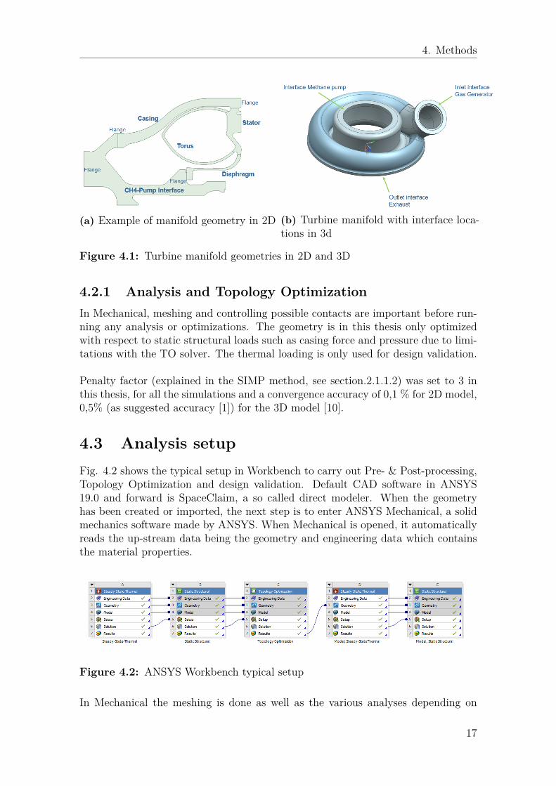
4.2 GeometryThe different parts shown in Fig.4.1 are shortly explained here to bring an under-standing for the manifold. The manifold consists of a torus which is containing thecombusted LCH4 and LOX, pushing the hot gas in 360 down to the stator andfurther down the rotor. A diaphragm which is keeping the leakage flow of methane,on the bottom side of the CH4-Pump Interface, not to flow up-stream in the engine.The geometry in Fig.4.1a also consists of a casing, which purpose is to bring stiffnessto the manifold. The casing is not present in the Fig.4.1b, instead the diaphragmhas been increased in thickness. The manifold has several interfaces, the flanges, ascan be seen in Fig.4.1a and Fig.4.1b.

16

4. Methods

(a) Example of manifold geometry in 2D (b) Turbine manifold with interface loca-tions in 3d

Figure 4.1: Turbine manifold geometries in 2D and 3D

4.2.1 Analysis and Topology OptimizationIn Mechanical, meshing and controlling possible contacts are important before run-ning any analysis or optimizations. The geometry is in this thesis only optimizedwith respect to static structural loads such as casing force and pressure due to limi-tations with the TO solver. The thermal loading is only used for design validation.

Penalty factor (explained in the SIMP method, see section.2.1.1.2) was set to 3 inthis thesis, for all the simulations and a convergence accuracy of 0,1 % for 2D model,0,5% (as suggested accuracy [1]) for the 3D model [10].

4.3 Analysis setupFig. 4.2 shows the typical setup in Workbench to carry out Pre- & Post-processing,Topology Optimization and design validation. Default CAD software in ANSYS19.0 and forward is SpaceClaim, a so called direct modeler. When the geometryhas been created or imported, the next step is to enter ANSYS Mechanical, a solidmechanics software made by ANSYS. When Mechanical is opened, it automaticallyreads the up-stream data being the geometry and engineering data which containsthe material properties.

Figure 4.2: ANSYS Workbench typical setup

In Mechanical the meshing is done as well as the various analyses depending on

17

4. Methods

what analysis systems are linked together in workbench. In Fig. 4.2 three analysissystems are linked together, the first three are Steady-sate thermal, static structuraland topology optimization. The later two are coupled only to read the results fromthe topology optimization in order to perform a design validation. When meshingis done in Mechanical and the loadcases are applied and evaluated, the topologyoptimization can be initiated.

In the TO analysis system the objective, response constraints and manufacturingconstraints are defined as well as what solver to be used, what region to be opti-mized and what region to be excluded. For example, aerodynamic surfaces are notan option to optimize. So they are kept untouched by choosing them as exclusionregion.

The file format of a finished TO-geometry for post-processing is STL (Stereolithog-raphy) and contains faceted data. The faceted geometry has to be post-processed inorder to smooth out sharp edges and possibly correct bad geometry before carryingout the design validation.

4.3.1 Preparing the Topology Optimization AnalysisWhen preparing geometry for Topology Optimization it’s usually necessary to addsome wrapping (or packing) geometry depending on what areas one wants to opti-mize. In Fig.4.3 the geometry is given a packing volume in order to find an alter-native solution to the diaphragm and casing. The geometry is thus given a largewrapping volume so that new load paths can be created when subjected to a loadcase.

Preprocessing can be done in any CAD software. In this thesis ANSYS SpaceClaimand Siemens NX has been used.

(a) Original geometry (b) Original geometry with packing vol-ume

Figure 4.3: Preprocessing example in SpaceClaim of geometry for a certain 2Dcase

18

4. Methods

4.3.2 Boundary Conditions and LoadsThere exists in total five loads and two thermal boundary conditions, relevant forthe manifold optimization, which are listed in Tab. 4.2 and visualized in Fig. 4.4.For the 2D case, only the exhaust force, pressure and thermal boundary has beenconsidered whereas for the 3D model all loads are applied.

The manifold is constrained at the far left edge in the 2D-model, see Fig. 4.4a. Inthe 3D model it is constrained at the diaphragm interface, where it has been coloredblue, see Fig. 4.4b.

Table 4.2: Loads and boundary conditions for the manifold

Load type UnitInlet Force [N]Exhaust Force [N]Inlet Moment [Nm]Exhaust Moment [Nm]Pressure [Pa]Thermal boundary low (Tlow) [K]Thermal boundary high (Thigh) [K]

(a) Relevant loads for the 2D geometry (b) 3D geometry with all loads

Figure 4.4: Manifold in 2D and 3D with relevant loads

The inlet force and moment are loads due to the interface coupling between turbinemanifold and the gas-generator further up-stream in the engine. The exhaust forceand moment are similarly to the inlet, interface loads but here coupled to the heatexchanger. The magnitude of these loads are outputs from a more complete engineanalysis where the whole engine has been assembled.

The gas generator delivers combusted propellant to the manifold of extreme magni-tude in pressure. The hot gas is affecting the torus such that it wants to expand inall directions. The deformation of the torus has to be minimal as physical contactbetween e.g. casing and the torus could potentially cause devastating outcome in areal rocket launch.

19

4. Methods

Thermal gradients occur in the manifold as a result of the torus becoming very hotand the LCH4-pump-interface being very cold. These gradients can induce stressesby a factor 100 higher than the exhaust force, or a factor 3 higher stresses than forthe pressure load, meaning that this load is making a bigger impact on the designthan the others.

4.3.3 Topology Optimization parameters and constraintsIn this section all parts of the topology optimization system are explained. Analysissettings, design region, objective, response and manufacturing constraints to be ableto understand the results.

4.3.3.1 Analysis settings

In the analysis settings of the topology optimization system it is possible to definesome input settings for the solver. Maximum number of iterations is an option thatis set to 500 by default but can be changed to another desired number. The solverwill iterate until it converges or until it has been iterating the maximum amount oftimes and is interrupted.

For numerical reasons, the density of an element cannot be exactly zero. The min-imum normalized density has to be specified and it can be of any value between 0and 1.By default it is set to 0.001 and is kept like that throughout this thesis.

The convergence accuracy has to be specified to be equal to 2% or less, default isse to 0.1 %. If the objective, explained in section 4.3.3.3, is to minimize mass orvolume (in combination with a Von-Mises stress constraint) it is recommended toset the value to 0.05 % or lower.

Explained in the SIMP method, see section 2.1.1.2, the penalty factor has to bespecified in order to steer the solution to a 0-1 optimized geometry. The penaltyfactor is recommended by Bendsø et.al [1] and ANSYS in [26], to be set to 3. Thisis to prevent the structural stiffness matrix to not scale linearly with the pseudodensity. In this thesis the penalty factor has been equal to 3.Lastly in the Analysis settings the solver, further explained in section 2.1.2, has tobe chosen. In this thesis the solver Sequential Convex Programming has been used.

4.3.3.2 Optimization Region

The region to be optimized is controlled by defining the design and exclusion re-gions. The design region is allowed to be optimized whilst the exclusion region is afixed geometry and cannot be optimized by the solver.

In this thesis, the inside of the torus is always kept as an exclusion region as itis important to not change any aerodynamic surfaces for the performance of theturbine. All boundary conditions automatically becomes exclusion regions, but theremight exist additional geometry that cannot be optimized.

20

4. Methods

4.3.3.3 Objective

The purpose of the topology optimization is its objective. The objective is oftena minimization problem where in ANSYS there exists three different objectives forstatic structural linear optimization. The most common is to minimize compliance,which is a synonym for maximizing the stiffness, this is further explained in section2.1.1.1. Minimizing volume or mass are the other two objective options.

If the geometry is optimized with a linked modal system, then the objective is bydefault to maximize the frequency or minimize for mass or volume.

It is possible to do a topology optimization with several objectives, if a modal systemand a static structural system are linked together, then the topology optimizationsystem reads and iterate over both systems. As there are two linked systems, twoobjectives can be defined, for example maximizing frequency and minimizing com-pliance. It is possible to link more than two systems together.

4.3.3.4 Response Constraints

The desired response during an optimization can be controlled by its response con-straints. For mass and volume there exist an option to specify the amount, inpercent, to retain of the design region. In the stress constraints the possibility todefine the maximum allowed stress either locally or globally is set. In this thesis thestress constraints are used to not allow the optimized geometry to exceed the yieldpoint with some margin.

Table 4.3: Response constraints supported by ANSYS TO solvers

Constraint type EnvironmentMass Modal & Static StructuralVolume Modal & Static StructuralGlobal von-Mises Stress Static StructuralLocal von-Mises Stress Static StructuralNatural Frequency ModalDisplacement Static StructuralReaction Force Static Structural

The mass or volume to retain has been altered in this thesis between 50 and ∼ 5%and the Global von-Mises stress constraint to less than the yield point with somemargin.

4.3.3.5 Manufacturing Constraints

If a component is not to be manufactured through additive manufacturing thenthere might be constraints on what geometry actually is possible to manufacture.ANSYS has a set of manufacturing constraints which, if defined, the solver has totake into account when optimizing the geometry.

21

4. Methods

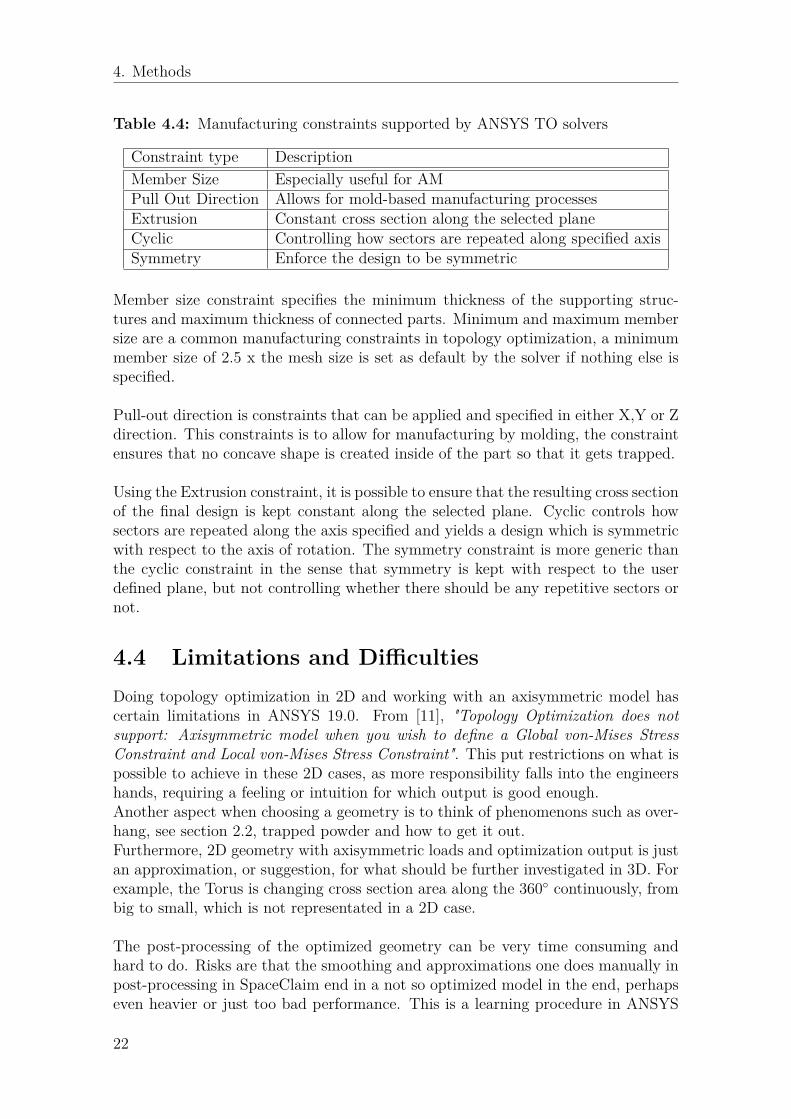
Table 4.4: Manufacturing constraints supported by ANSYS TO solvers

Constraint type DescriptionMember Size Especially useful for AMPull Out Direction Allows for mold-based manufacturing processesExtrusion Constant cross section along the selected planeCyclic Controlling how sectors are repeated along specified axisSymmetry Enforce the design to be symmetric

Member size constraint specifies the minimum thickness of the supporting struc-tures and maximum thickness of connected parts. Minimum and maximum membersize are a common manufacturing constraints in topology optimization, a minimummember size of 2.5 x the mesh size is set as default by the solver if nothing else isspecified.

Pull-out direction is constraints that can be applied and specified in either X,Y or Zdirection. This constraints is to allow for manufacturing by molding, the constraintensures that no concave shape is created inside of the part so that it gets trapped.

Using the Extrusion constraint, it is possible to ensure that the resulting cross sectionof the final design is kept constant along the selected plane. Cyclic controls howsectors are repeated along the axis specified and yields a design which is symmetricwith respect to the axis of rotation. The symmetry constraint is more generic thanthe cyclic constraint in the sense that symmetry is kept with respect to the userdefined plane, but not controlling whether there should be any repetitive sectors ornot.

4.4 Limitations and DifficultiesDoing topology optimization in 2D and working with an axisymmetric model hascertain limitations in ANSYS 19.0. From [11], "Topology Optimization does notsupport: Axisymmetric model when you wish to define a Global von-Mises StressConstraint and Local von-Mises Stress Constraint". This put restrictions on what ispossible to achieve in these 2D cases, as more responsibility falls into the engineershands, requiring a feeling or intuition for which output is good enough.Another aspect when choosing a geometry is to think of phenomenons such as over-hang, see section 2.2, trapped powder and how to get it out.Furthermore, 2D geometry with axisymmetric loads and optimization output is justan approximation, or suggestion, for what should be further investigated in 3D. Forexample, the Torus is changing cross section area along the 360 continuously, frombig to small, which is not representated in a 2D case.

The post-processing of the optimized geometry can be very time consuming andhard to do. Risks are that the smoothing and approximations one does manually inpost-processing in SpaceClaim end in a not so optimized model in the end, perhapseven heavier or just too bad performance. This is a learning procedure in ANSYS

22

4. Methods

that the engineer has to get feeling for. Further, exporting the "correct" geometrywith respect to the chosen density threshold can also be quite tricky, where a rule ofthumb is to at least choose an element density where the geometry starts to connectwith eachother.

Another limitation is that the stator is not quite representative in these analyses.As the stator is not solid through the 360, but perhaps just 30% mass in a 3D case.The material data can be seen as a limitation as well, being only an approximatelinear case.

4.4.1 Finite Element Solution work flowWhen initiating the analysis, the first step is to set up the geometry and apply theFE-mesh. Then, boundary conditions, loads, objective and response constraints areapplied. The solver usually starts by giving all elements in the mesh a uniformdistribution of densities (e.g ρ = 0.6) and then starts the optimization loop. Thefirst step in this iterative process is solving the equilibrium equations as in Eq.(2.6)using FE discretization and linear solver, followed by sensitivity analysis calculat-ing derivatives of the objective function, taking into account the design variables.Filtering techniques are applied before updating the densities

Figure 4.5: The general work flow scheme of Topology Optimization, courtesy ofShun Wang [7]

23

4. Methods

This procedure will iterate a number of times until the solution has converged andthe final topology can be studied and post-processed.

4.4.2 Post-processing and design validationThe TO geometry can be exported from Mechanical as an .STL file, being a facetedgeometry and not a solid. The surfaces and features are rough (depending on meshsize) and need to be smoothed before sent to an AM printer or before doing furtheranalysis. SpaceClaim is a great software for cleaning up the geometry and creatingsmooth surfaces and solids from the faceted data, it has been used in the interme-diate step in this thesis to prepare the model for validation. SpaceClaim consistsof several well suited tools for working with facets, such as Auto Fix, Shrinkwrap,smoothing tools and more. These has been used to a great extent but will not befurther explained in this thesis.

Workbench has an option called "transfer to design validation system" which is veryneat for post-processing possibilities. Faceted data as well as the original geometryis exported to a new linked system being a copy of the original. The original ge-ometry together with the TO faceted geometry makes it easier to post-process asfeatures from the original geometry can easily be applied on the TO geometry.

It was realized during the thesis work that repairing faceted 3D geometry (especiallywhen the original geometry has been created from splines etc.) is very hard and timeconsuming to work with. Thus, no more post-processing than absolute necessarywas done for 3D geometry in order to save time. For 2D geometry it is much easieras very often a sketch plane can be created and curves extracted from the faceteddata and then smoothing the curves is quite easy.

When the post-processing in SpaceClaim is done, it is possible to open up theMechanical environment in the copy of the analysis system that was generated whentransferring to design validation. Here all settings for mesh, loads etc. are copiedfrom the original system so that an easy validation of the structure created can bedone and compared with the initial one.

4.5 2D StudyWorking in 2D has several advantages such as quick simulations, easier post-processingand interpretation compared to a 3D case. But it also has several limitations as thesoftware is not as developed for 2D cases as for 3D. As mentioned before, makingconstraints on stress is not optional for an axisymmetric model in 2D. In ANSYSWorkbench 19.0 there is also a limitation that the "transfer to design validation" isnot working for axisymmetric models, ANSYS later confirmed that this most likelyis a bug.

24

4. Methods

4.5.1 Load casesFor the 2D study the idea is to apply relevant loads to see whether the topologyoptimization can find new designs for the casing and diaphragm. This can be donevery quickly compared to a 3D case and thus the behaviour of the geometry andloads can be investigated so that no meaningless and time-consuming simulationsare done later in 3D.

As the solver is iterating FE-analyses every time the design is updated in the loop,it directly sees where material should be added or removed. The relevant loadsare exhaust force, torus pressure, thermal loading and are previously explained inFig.4.4a.

4.5.2 Design approachThere are several ways of designing the manifold to meet the requirements providedby the customer. Depending on what design space you give the model, the outcomewill be different.

One approach is to have a casing to bare the axial loads together with the samesetup as explained in section 4.3.2, and visualized in Fig. 4.1a. The geometry isthus given a design space as in Fig. 4.6 so that the solver has the possibility tocreate an optimized casing.

Another approach is to skip the casing and have a bigger, stiffer diaphragm as weightreduction could be achieved as well as possible mitigation of modal issues with theouter casing, see Fig. 4.7. If no casing is of interest during the optimization, thenneither is a design space of interest in that area.

4.5.3 CasingThe first approach of this thesis was to optimize the casing and diaphragm by fillingup all empty space between the parts, see Fig. 4.6, and let the program, withconstraints and loads, find the optimal geometry.

25

4. Methods

Figure 4.6: Example of manifold with added geometry for Topology Optimization

Here in Fig. 4.6 the design space is not touching the Torus because of thermalisolation reasons.The TO analysis system is then linked with the static structural system and possiblySteady-state thermal system to see the loads and for which the final geometry shouldwork for.

4.6 Capable DiaphragmAs costs is the major driving factor of this project there is an interest to skip theouter casing and have a more capable diaphragm to bare all the loads.

26

4. Methods

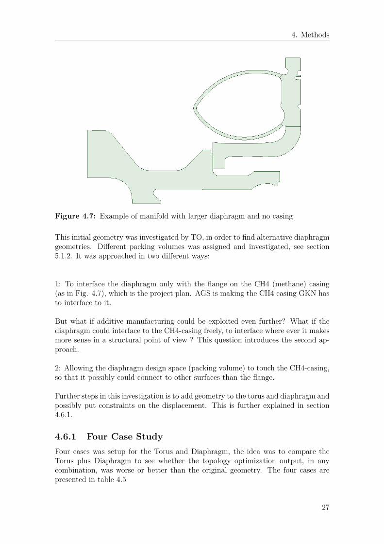
Figure 4.7: Example of manifold with larger diaphragm and no casing

This initial geometry was investigated by TO, in order to find alternative diaphragmgeometries. Different packing volumes was assigned and investigated, see section5.1.2. It was approached in two different ways:

1: To interface the diaphragm only with the flange on the CH4 (methane) casing(as in Fig. 4.7), which is the project plan. AGS is making the CH4 casing GKN hasto interface to it.

But what if additive manufacturing could be exploited even further? What if thediaphragm could interface to the CH4-casing freely, to interface where ever it makesmore sense in a structural point of view ? This question introduces the second ap-proach.

2: Allowing the diaphragm design space (packing volume) to touch the CH4-casing,so that it possibly could connect to other surfaces than the flange.

Further steps in this investigation is to add geometry to the torus and diaphragm andpossibly put constraints on the displacement. This is further explained in section4.6.1.

4.6.1 Four Case StudyFour cases was setup for the Torus and Diaphragm, the idea was to compare theTorus plus Diaphragm to see whether the topology optimization output, in anycombination, was worse or better than the original geometry. The four cases arepresented in table 4.5

27

4. Methods

Table 4.5: Four cases, Diaphragm and Torus study

Case Diaphragm TorusCase 1 Original OriginalCase 2 Original OptimizedCase 3 Optimized OriginalCase 4 Optimized Optimized

These four cases where then validated and compared with each other, case 1 is actingas a reference.

4.7 3D StudyFrom previous work done at GKN it was well known that the current configurationof design and loads made the material, Inconel 718, exceed the yield point at severallocations. Some of these loads are not representative in a 2D case and thus need tobe modeled and analyzed in 3D.

The area of most interest is the gas generator interface causing high stresses on theinlet geometry, seen on the right hand side in Fig. 4.8a.

(a) Top view (b) Bottom view

Figure 4.8: Nominal manifold geometry

Sometimes it can be hard to visualize the optimized structure in Mechanical assection cuts do not work for TO output, thus one has to make use of a "user definedresult" in Mechanical called TOPO or ETOPO. When this result is added, all initialgeometry is visualized and color coded depending on what density they got in theend of the simulation. Blue color means that the density is minimum (0.001) andred means it is maximum density. Intermediate densities are the colors in between.Looking at a cross section of the geometry is then possible. Densities shown herewhich are lower than the chosen density threshold will not be present when exportingthe geometry.

28

4. Methods

4.7.1 Design approachModifying the current design by adding a design space around the inlet interfacewas known to be necessary as from previous analyses done on site showed stressesover the yield point especially in this area. That resulted in a manifold with addeddesign space, as shown in Fig. 4.9. To cut down on simulation time the nozzles(turbine stator) was replaced with a solid disk of material to contribute with stiff-ness, but keeping the amount of mesh elements down. The same reason goes for theflanges, which got their bolt holes removed. As can be seen especially from the Fig.4.9b,material around the gas generator interface has also been added with cut-outsfor external geometry interference reasons.

Another approach was to fully enclose the manifold so that geometry between di-aphragm and the torus could be created in the optimization procedure. This wasdone for a model with the stators still in place, see Fig. 4.10.

(a) Top view (b) Bottom view

Figure 4.9: Added design space around inlet interface

29

4. Methods

(a) Front view (b) Side view

(c) Bottom view (d) Design region

Figure 4.10: Fully enclosed manifold

4.7.2 LoadsThe loads are the same as for the 2D analysis, plus external force and moment onthe inlet interface (Gas generator) and exhaust. These loads are defined by ArianeGroup, derived from a complete engine analysis and are a consequence of functionalloads, quasi-static loads and dynamic loads experienced in flight. The loads are Ef-fort [N], which is a vector force F = [X, Y, Z] and a Moment [N.m], M = [X, Y, Z].The vector force is applied as a "spider load", or as called in ANSYS Mechanical, a"Remote Force". The interface between the turbine manifold and pump is clamped(Fixed support) for all load cases.

The loads for the case with added geometry around the inlet are the same as for thefully enclosed manifold.

30

4. Methods

Figure 4.11: Manifold with loads applied and added inlet geometry

Figure 4.12: Fully enclosed manifold with loads applied

31

4. Methods

32

5Results

Due to confidential data the exact dimensions and values achieved in simulationscannot be presented here. Instead, normalizing the values and comparing them toeach other is done to understand the outcome.

5.1 2DIt was realized that thermal loading was not an option to include for the TO itself,as the "Steady State Thermal Analysis" is not a supported analysis system for theTO-loop. Initially, it was thought to be possible to import the induced stresses fromthermal analysis into the static structural as nodal loads. However, these loads arenot iterated and updated as the solver progresses but are simply kept constant.When optimizing for thermal loads the outcome were often free-floating geometryas in Fig.5.3e, thus being unfeasible results from a structural point of view.

5.1.1 Casing DesignsThe design space was setup as in Fig. 5.1, to find an optimal casing geometry aswell as an optimal diaphragm for different load cases described in Ch. 4.

The different load cases where applied and TO settings kept identical for all casesto understand the main differences in TO for different loads. The topology opti-mization results can be seen in Fig.5.3. On the right hand side of these figuresthe density for all elements are plotted in a contour plot, where red colour meansthat the material has a pseudo density of ρ = 1 and blue ρ = 0.001. On the lefthand side only densities of ρ ≥ 0.5 is shown as it is a user set parameter, see Tab. 5.1.

For figures showing the design region of the model, the blue and red color is simplyto distinguish between design and exclusion region, see Fig.5.1.

33

5. Results

Figure 5.1: Design region for TO of casing and diaphragm

In Fig. 5.2 the stresses for the different load cases have been visualized through-out the entire structure including the design space. An indication of where masswill later achieve higher pseudo densities performing the topology optimization. InFig.5.2a), Exhaust load, most of the stress can be seen at the top part of the ge-ometry, indicating material is needed there. For Fig.5.2b most of the stress is forthe torus, for the thermal load in Fig.5.2c) most of the stress occurs at the interfacebetween diaphragm and the stator. Lastly, for load case 4, the pressure load isclearly dominant over the exhaust load as almost all stress is seen around the torus,Fig. 5.2d.

The TO is then initialized with the objective to minimize compliance and the re-sponse constraint to retain 20% mass as we want the outcome to be in the same rangeas for the nominal geometry, see Fig.4.3a. The result is then shown for elementswith a ρ ≥ 0.5.

34

5. Results

(a) Load Case 1 - Exhaust load (b) Load Case 2 - Pressure load

(c) Load Case 3 - Thermal load (d) Load Case 4 - Exhaust load & pressureload

Figure 5.2: Equivalent von-Mises Stress contour plot for the different loadcases

Table 5.1: Parameters for TO with different loadcases

Type MaxRetained Mass 20 %Density (ρ) 0.5

35

5. Results

(a) Load Case 1, TO result (b) Load Case 1, ETOPO, countour plotof the TO geometry

(c) Load Case 2, TO result (d) Load Case 2,ETOPO, countour plotof the TO geometry

(e) Load Case 3, TO result (f) Load Case 3, ETOPO, countour plotof the TO geometry

(g) Load Case, 4 TO result(h) Load Case 4, ETOPO, countour plotof the TO geometry

Figure 5.3: Difference in TO for the four loadcases

The outcome shows that the exhaust load (load 1) is finding load paths (and thus

36

5. Results

a structure) in what could become a casing, whilst the pressure load (load 2) isfinding load paths through the diaphragm more optimal. In Fig. 5.3a more impor-tance seems to be for the casing structure than for the diaphragm. In Fig. 5.3c forthe pressure load, more importance is for the diaphragm, leaving the outer casingstructure to a minimum. Load 3 (thermal loading) in Fig. 5.3e the geometry isbreaking up as explained earlier, the result is not feasible from a structural point ofview. Lastly in Fig. 5.3g where both casing load and pressure load is present thereis a clear dominance in the importance of a bigger diaphragm than an outer casing.

The results are feasible due to the magnitude of the loads. However, the pressureinside of the torus is of greater magnitude than for the exhaust load which can beseen in Fig. 5.2d.

From these results the most important outcome is that the diaphragm seem to be ofmost importance for the structural integrity. The diaphragm is further investigatedin section 5.1.2.

5.1.2 Four Case Study - Comparing Diaphragm and TorusThe idea of the diaphragm and torus study originates in that a casing for the man-ifold is heavy and expensive. This gave birth to the idea to make the diaphragmbigger, thus stiffer, to bare the loads alone. The manifold was therefore studied andcompared with various cases.

Design validation must always follow the optimization analysis to conclude whetherthe result seams feasible or not. Feasible in a sense how original geometry stressesand deformations have changed in comparison to the new optimized geometry. Theoriginal geometry looks like in Fig. 4.7, where the diaphragm is significantly largerthan in Fig. 4.1a. The comparison is as in Tab. 4.5 and presented in followingsections.

In these different test cases Load 1 represents the exhaust load, load 2 the toruspressure and Load 3 the thermal loading.

5.1.2.1 Case 1 - Original Diaphragm and Original Torus

The geometry in Fig. 4.1a will act as the nominal geometry. Therefore, only astructural analysis is needed which main purpose is to act as a comparison referencefor the following cases. The loads are applied and results in the following pictures,see Fig. 4.3a.

Hereinafter, in the comparative study, the maximum stress and deformation will becompared relatively to this case, being the nominal for the Four Case Study.

37

5. Results

(a) Equivalent Von-Mises Stress (b) Total Deformation

(c) Steady-state Thermal

Figure 5.4: Stress, Deformation and Thermal plots of the original geometry

5.1.2.2 Case 2 - Original Diaphragm and Optimized Torus

The torus is increased in thickness by making an offset on the outer radius. Dueto the non-homogeneous shape, there where difficulties in increasing the thicknessby the exact amount everywhere. Thus the offset varies between 66 % and 125% inincreased thickness. The model is then analyzed for the casing load and pressureload.

38

5. Results

(a) Equivalent Von-Mises Stress (b) Total Deformation

(c) Steady-state Thermal

Figure 5.5: Stress, Deformation and Thermal plots of the original geometry withan extra 66 to 125 % thicker Torus

The outcome is max stress of 54.79 % of the original geometry, case 1, and 10.35% of the original deformation.The mass is however 112.19 % of the nominal, due tothe thicker Torus. The TO analysis system is then run and set with the parameterspresented in Tab. 5.2.

Table 5.2: Parameters for TO of Torus

Objective Minimize Compliance Retained ThresholdResponse Constraint Mass 50% , 40% , 30%Manufacturing Constraint None N/A

39

5. Results

(a) Design (blue) and exclusion region(red)

(b) Mass Retained 50 %, ρ =0,35

(c) Mass Retained 40 %, ρ =0,35 (d) Mass Retained 30 %, ρ =0,30

Figure 5.6: TO for the offset Torus

The most suitable optimized geometry to be post-processed and validated was de-cided to be Fig. 5.6c. Due to the geometry still being connected in a frameworkstructure and not breaking up. After post-processing, the TO geometry was trans-ferred to design validation with the following output.

(a) Equivalent Von-Mises stress (b) Total deformation

Figure 5.7: Design validation of the TO Torus

40

5. Results

Figure 5.8: Zoomed in on equivalent von mises stress, local maxima observed inred

Far left of torus and near the stator (right hand side) local maxima can be observed.

Table 5.3: Design validation of TO Torus compared to nominal geometry

Type MaxEquivalent Von-Mises Stress 102.82 %Total Deformation 90.14 %Retained mass 102.53%

The maximum stress increased by almost 3 % compared to the nominal geometrybut the total deformation is almost 10 % less. The final weight of the component ishowever 2.5 % heavier than the nominal weight. Several local maximum stresses canbe seen. To manufacture this Torus would also impose difficulties with extractingthe trapped powder in the cavities.

5.1.2.3 Case 3 - Optimized Diaphragm and Original Torus

The diaphragm is optimized by setting up the design space as in the followingpicture. Where only the blue colored geometry were allowed to be optimized.

41

5. Results

(a) Design (blue) and exclusion region(red)

(b) Mass Retained 14 %, ρ = 0.4

Figure 5.9: TO for the Diaphragm

The geometry was post-processed in SpaceClaim and then forwarded to design val-idation.

(a) Equivalent Von-Mises stress (b) Total deformation

Figure 5.10: Design validation of the TO Diaphragm

The results are presented in Tab. 5.4.

Table 5.4: Design validation of TO diaphragm compared to nominal geometry

Type MaxEquivalent Von-Mises Stress 163,67 %Total Deformation 125.85 %Retained mass 95.20 %

The weight of the optimized geometry is 4.80 % less but quite significant higherstresses, found to be from local maximum.By smoothing out the edges for the diaphragm voids, lower deviations from thenominal values was achieved for both the stress and deformation, but a slight increasein mass. See Fig. 5.11 and Tab. 5.5.

42

5. Results

(a) Equivalent Von-Mises stress (b) Total deformation

Figure 5.11: Design validation of the smoothed TO Diaphragm

Table 5.5: Design validation of smoothed TO diaphragm compared to nominalgeometry

Type MaxEquivalent Von-Mises Stress 113.28 %Total Deformation 122.55 %Retained mass 95.86 %

This is an example of the importance for design validation and post-processing, theoptimized geometry indicates where mass could be removed and in post-processingthe result is interpreted and modified. The design validation is then further indicat-ing whether more post-processing is needed or not. In this case, further smoothingout the cavities resulted in lowering stresses by 50 %.

43

5. Results

5.1.2.4 Case 4 - Optimized Diaphragm and Optimized Torus

The diaphragm from case 3 together with torus from case 2 are set together intoone geometry and evaluated.

(a) Equivalent Von-Mises stress (b) Total deformation

Figure 5.12: Design validation of the TO Diaphragm and TO Torus together

Table 5.6: Design validation of TO diaphragm and TO Torus compared to nominalgeometry

Type MaxEquivalent Von-Mises Stress 194.57 %Total Deformation 115.93 %

As maximum stresses occure at sharp edges and corners the diaphragm and Toruswas smoothed even more.

(a) Equivalent Von-Mises stress (b) Total deformation

Figure 5.13: Design validation of further smoothed TO Diaphragm and TO Torustogether

The smoothing resulted in lower max stress and deformation as can be seen in table5.7.

44

5. Results

Table 5.7: Design validation of smoothed TO diaphragm and TO Torus comparedto nominal geometry

Type MaxEquivalent Von-Mises Stress 104.61%Total Deformation 113,66%Retained mass 99.37%

5.1.2.5 Case 4 - Extended Work

Less offset Torus, now only about 4mm in average thickness. Diaphragm second"void" increased in order to reduce mass, compare Fig. 5.14a and Fig. 5.14b.

(a) Design (blue) and exclusion region (red)(b) Mass Retained 50 %, ρ =0,35 OnTorus, then increased right most void atdiaphragm

(c) Equivalent Von-Mises stress (d) Total deformation

Figure 5.14: TO for the 4 mm offset Torus with an increased right most void

Table 5.8: Design validation of further smoothed TO diaphragm and TO Toruscompared to nominal geometry

Type MaxEquivalent Von-Mises Stress 111.03%Total Deformation 119.96%Retained mass 94.17%

45

5. Results

Almost 6 % Lower mass than nominal, but a bit higher stress and deformation isthe outcome from this analysis.

Topology optimization in 2D has from these studies been found to be hard due to thelack of using stress constraints which is not supported for 2D axisymmetric models.

5.2 3DThe nominal geometry is put under the load cases to get an intuition of where ma-terial is needed. The result in Fig. 5.15, are stresses (red and yellow) 150% to 200%over the acceptable level.

When doing topology optimization in 3D it is possible create response constraints onthe global Von-Mises stress, this was done for all TO cases to not be over the yieldpoint, with some margin. Thus 800 MPa was chosen as an appropriate maximumglobal von-Mises stress constraint. The stress plot in Fig. 5.15 indicates that extrastiffness around the inlet is necessary.

(a) Front view. Total Von-Mises Stress (b) Side view. Total Von-Mises Stress

(c) Side view. Total Deformation

Figure 5.15: Nominal geometry contour plot of stress and deformation

46

5. Results

5.2.1 Inlet OptimizationIn Fig. 5.16, TO with objective to minimize compliance, manufacturing constraintsminimum member size of 15 mm, maximum member size of 25mm, ρ = 0.59 ispresented. Here, only the material added around the inlet has been optimized, itbecame 16 % heavier than the nominal geometry. As expected from Fig. 5.15,material is kept especially around the areas with high stress and deformation.

(a) Front view (b) Zoomed side view

(c) Zoomed side top view (d) Design region

Figure 5.16: Topology optimization of only the added inlet geometry

Table 5.9: Inlet optimization parameters for Fig. 5.16, 16 % heavier than nominal.

Type MaxObjective Minimize ComplianceResponse constraint 20% massMinimum & Maximum membersize 15 [mm] & 25 [mm]Maximum global Von-Mises stress 1000 MPaPseudo Density, ρ 0.59

In the case of Fig. 5.17, the program was allowed to work with more geometrythan only for the inlet to see whether the rest of the manifold was over-designed.

47

5. Results

As a result the program did not change the torus at all, subtracting some fromthe diaphragm and a lot of material is kept on the top of the inlet where extramaterial was assigned. In Fig. 5.17c a cross section of the ETOPO result is made tovisualize the framework structure created around in the inlet of the manifold. Thefinal weight is 5.67 % heavier than the nominal geometry.

(a) Top view (b) Side view, zoomed

(c) ETOPO cross section of inlet (d) Design region

Figure 5.17: TO for inlet, diaphragm and torus for ρ = 0.59

Table 5.10: Inlet, torus and diaphragm optimization parameters for the case inFig. 5.17. 5.67 % heavier than nominal

Type MaxObjective Minimize ComplianceResponse constraint 30% massMinimum & Maximum membersize 15 [mm] & 25 [mm]Maximum global Von-Mises stress 800 MPaPseudo Density, ρ 0.59

The program was pushed further by pushing the Response constraint down to 10 %to meet weight requirements. The results is a manifold of 91.03 % of the nominalone, meaning the total weight is reduced by about 9 % and structural integrity iskept. A lot of material is subtracted from the added geometry on the inlet, as wellas geometry on the diaphragm. Making the diaphragm thinner.

48

5. Results

(a) Top view (b) Top view, zoomed

(c) Side view, zoomed (d) Bottom view

(e) ETOPO, to illustrate diaphragm re-duction

(f) ETOPO of inlet geometry

Figure 5.18: TO for inlet, diaphragm and torus for ρ = 0.5

Table 5.11: Inlet, torus and diaphragm optimization parameters for the case inFig. 5.18, 9 % lighter than nominal

Type MaxObjective Minimize ComplianceResponse constraint 10% massMinimum & Maximum membersize 15 [mm] & 25 [mm]Maximum global Von-Mises stress 800 MPaPseudo Density, ρ 0.5

49

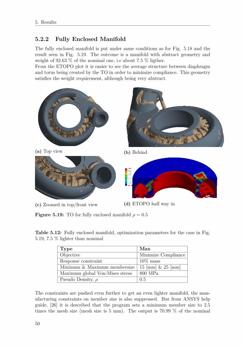
5. Results

5.2.2 Fully Enclosed ManifoldThe fully enclosed manifold is put under same conditions as for Fig. 5.18 and theresult seen in Fig. 5.19. The outcome is a manifold with abstract geometry andweight of 92.63 % of the nominal one, i.e about 7.5 % ligther.From the ETOPO plot it is easier to see the average structure between diaphragmand torus being created by the TO in order to minimize compliance. This geometrysatisfies the weight requirement, although being very abstract.

(a) Top view (b) Behind

(c) Zoomed in top/front view (d) ETOPO half way in

Figure 5.19: TO for fully enclosed manifold ρ = 0.5

Table 5.12: Fully enclosed manifold, optimization parameters for the case in Fig.5.19, 7.5 % lighter than nominal

Type MaxObjective Minimize ComplianceResponse constraint 10% massMinimum & Maximum membersize 15 [mm] & 25 [mm]Maximum global Von-Mises stress 800 MPaPseudo Density, ρ 0.5

The constraints are pushed even further to get an even lighter manifold, the man-ufacturing constraints on member size is also suppressed. But from ANSYS helpguide, [26] it is described that the program sets a minimum member size to 2.5times the mesh size (mesh size is 5 mm). The output is 70.99 % of the nominal

50

5. Results

geometry, meaning there is a weight reduction of about 29 %.The structure createdbetween torus and diaphragm in Fig. 5.20 compared to in Fig. 5.19 is of smallercharacter and greater amount. This is due to the member size constraint not beingused here, allowing the structure to be of any (program controlled) minimum andmaximum size. Further, there is no structure around the inlet geometry as in Fig.5.19c because of the response constraint being lowered to 7%.

(a) Top view(b) Behind

(c) Zoomed in top/front view

(d) ETOPO half way in

Figure 5.20: TO for fully enclosed manifold with program controlled member size,ρ = 0.5

Table 5.13: Fully enclosed manifold, optimization parameters for the case in Fig.5.20, 29 % lighter than nominal

Type MaxObjective Minimize ComplianceResponse constraint 7% massMinimum & Maximum membersize Program controlled & Program controlledMaximum global Von-Mises stress 800 MPaPseudo Density, ρ 0.5

It becomes hard to visualize the structure created between torus and diaphragm fromthe topology optimization when a member size constraint is not applied. The model

51

5. Results

is also hard to post-process due to the number of supporting structure, meaningmore faceted data. The model is thus given a minimum member size of 15 mm andprogram controlled maximum member size. Thus, there is no specified maximumlimit, and larger sectors of structure can be created. To make the topology opti-mization output even more simplified, an extrusion constraint in X-axis is appliedto achieve a constant cross section in the plane.

(a) Top view (b) Behind

(c) Zoomed top/front view (d) ETOPO half way in

Figure 5.21: TO for fully enclosed manifold with extrusion constraint, ρ = 0.5

Table 5.14: Fully enclosed manifold, optimization parameters and extrusion forthe case in Fig. 5.21, 29.6 % lighter than nominal

Type MaxObjective Minimize ComplianceResponse constraint 7% massMinimum & Maximum membersize 15 [mm] & Program controlledMaximum global Von-Mises stress 800 MPaPseudo Density, ρ 0.5Extrusion X-axis

The topology optimized geometry in Fig. 5.21 has less complex support structurethan Fig. 5.20. Meaning, it will not be as difficult to post-process in SpaceClaimwhen preparing for design validation.

The results from these topology optimizations are that it is indeed possible to reducethe weight of the manifold due to structural loads. However, thermal loads are

52

5. Results

foreseen to have a big impact on the structure but are not supported by the solverat the time of this thesis. The structure created between torus and diaphragmwould most likely create big thermal gradients, meaning the structural integrity ofthe manifold could be threatened.

53

5. Results

54

6Conclusion

Optimizing the manifold to meet performance and weight requirements has beenproven to be possible, although quite tricky. The loads are of great magnitude andthat puts limitations on how much weight actually is possible to reduce whilst stillkeeping the structural integrity. What kind of design space is assigned to a model isimportant for the final outcome from the TO; small tweaks can have a big impact,especially for interfacing surfaces.

Models can sometimes have cavities after optimization, meaning there would be en-trapped powder requiring to be removed after printing. Designs like the optimizedtorus, with a lot of cavities, might be unfeasible due to the difficulties in extractingthe powder, see Sec.5.1.2.2 for more details.

Working in 2D is hugely beneficial before working with 3D due to the speed in sim-ulation time. It is although quite hard and tedious to not be able to put the stressconstraints on the axisymmetric model as it requires extra manual iterations. The2D topology optimized geometries indicates that the diaphragm is more importantthan the casing for structural integrity, meaning a robust diaphragm is sufficient, seeSec.5.1.1. It is important to smooth out sharp edges and corners from the faceteddata when post-processing before carrying out a design validation to mitigate localmaxima.

From structural analysis and design validations the pressure and thermal loadingare the most prominent. Since topology optimization in ANSYS currently does notsupport thermal loads the optimized result risk to become unfeasible. This phenom-ena presents itself well in Fig.5.21 where thermal stresses would be indispensable.

Reducing the weight of the manifold seems to be possible, thus achieving the designrequirement with margin whilst still keeping the global stress levels under the yieldlimit, see Sec.5.2.2 where the weight was reduced by 30%. Further, the optimizationindicated that the diaphragm could be reduced by about 50% as well. However,design validation is always necessary to confirm whether the results are feasible ornot.

55

6. Conclusion

56

7Further Work

Post-processing of the 3D geometry should be done to validate the optimizationoutput. Design validation was done for the 2D study but not for the 3D. However,it should be done to validate the optimized model, especially for the thermal load.

Topology optimization also supports modal analysis which should be included infuture optimization work to find a robust model. To integrate the manifold withadjacent parts such as gas generator, heat exchanger and fuel pump could be doneto achieve more realistic results.

A grid convergence study for the various TO results has not been investigated. Thisis something that should be done as it could lead to a more accurate results. Themember size constraint should be further investigated as well.

Simplifications on the fully enclosed manifold, such as substituting the stators witha solid disk, as done in the inlet optimization study, should be done to cut downon simulation time for the fully enclosed model. To mitigate the thermal gradientsthat would build up between diaphragm and torus in the fully enclosed manifold,the design space created could be offset from the torus slightly so that no connectinggeometry, between torus and diaphragm can be created as in Sec.5.2.2.

57

7. Further Work

58

Bibliography

[1] M.P Bendsøe, O. Sigmund. Topology Optimization. Theory, Methods and Ap-plications, 2nd ed. Lyngby, Denmark.

[2] Shiro Yoshida, Michell Truss: Shape Optimization vs Analytical Solution.SHONAN, R& D, Inc. #402 Shonan Homes, 3-19-17 Katase-Kaigan, Fujisawa,251-0035 Japan

[3] M.P Bendsøe, N Kikuchi. Generating Optimal Topologies in Structural DesignUsing A Homogenization Method. (North-Holland 1988).

[4] M.Zhou, G.I.N Rozvany. The COC algortihm, part II: Topological, geometricaland generalized shape optimization.1991.

[5] ISO/ASTM 52900:2015 (ASTM F2792) Additive manufacturing – General prin-ciples – Terminology

[6] Dheeraj Gunwant & Anadi Misra Topology Optimization of Continuum Struc-tures using Optimality Criterion Approach in ANSYS. G. B. Pant Universityof Agriculture and Technology, Pantnagar, India

[7] Shun Wang. Krylov Subspace MEthods for Topology Optimization on AdaptiveMeshes. B.Eng, Tsinhua University, 2002.

[8] Christo Dordlofva. Qualification of Metal Additive Manufacturing in Space In-dustry. Challenges for Product Development. Luleå University of Technology,2018

[9] Prometheus Rocket engine, https://www.esa.int/Our_Activities/Space_Transportation/Prometheus_to_power_future_launchers

[10] Sequential Convex Programming, ANSYS HELP Guide, 2018 https://ansyshelp.ansys.com/account/secured?returnurl=/Views/Secured/corp/v190/wb_sim/ds_topo_solvers.html

[11] ANSYS Topology Optimization Limitations, ANSYS HELP Guide, 2018.https://ansyshelp.ansys.com/account/secured?returnurl=/Views/Secured/corp/v190/wb_sim/ds_topo_opt_limitations.html

[12] Svanberg, K., The Method of Moving Asymptotes, a new method for struc-tural optimization, International Journal for Numerical Methods in Engineer-ing, 24:359-373, 1987.

[13] Svanberg, K.,A class of globally convergent optimization methods based onconservative convex separable approximations, SIAM Journal of Optimization,2002, 12, 555-573

[14] Svanberg, K.,MMA and GCMMA – two methods for nonlinear optimiza-tion,Optimization and Systems Theory, KTH, Stockholm, Sweden.

59

Bibliography

[15] Langelaar Matthijs,An additive manufacturing filter for topology optimiza-tion of print-ready designs,Structural and Multidisciplinary Optimization,55(3):871883.

[16] Inconel718, http://www.hightempmetals.com/techdata/hitempInconel718data.php

[17] S.Brodin, L.Forsberg, U.Palmnäs, Turbine design for Ariane 6 Vulcain Turbop-umps upgrades, GKN Aerospace Trollhättan.

[18] EOS M 400, https://www.eos.info/systems_solutions/metal/systems_equipment/eos_m_400

[19] EOS M 400 , Datasheet, https://cdn0.scrvt.com/eos/9f24ce9ec18a70d9/4273833e1840/EOS_System_Data_Sheet_EOS_M_400_EN_V3_web.pdf

[20] L. Krog, A. Tucker, G. Rollema, 2002. Application of topology, sizing and shapeoptimization methods to optimal design of aircraft components.

[21] Airbus a380 Altair Engineering http://web2.altairhyperworks.com/taking-500kg-from-the-airbus-a380

[22] Kaufmann M. Cost/ Weight Optimization of Aircraft Structures, KTH Schoolof Engineering Sciences, Stockholm, 2008.

[23] Conceptual design Prometheus, https://www.esa.int/spaceinimages/Images/2017/12/Prometheus_powering_future_launchers

[24] Sigmund, O. (1997). On the design of compliant mechanisms using topologyoptimization. Mechanics of Structures and Machines, 25(4):493.524.

[25] ANSYS WorkBench User’s Guide https://ansyshelp.ansys.com/account/secured?returnurl=/Views/Secured/corp/v190/wb2_help/wb2_help.html

[26] ANSYS Mechanical User’s Guide https://ansyshelp.ansys.com/account/secured?returnurl=/Views/Secured/corp/v190/wb_sim/ds_Home.html

[27] About NX Software, Siemens PLM Software, https://docs.plm.automation.siemens.com/tdoc/nx/10/nx_api/#uid:index

[28] HyperWorks Online Help, Altair, http://www.altairhyperworks.com

60

AAppendix TOM

Previous topology optimization work at GKN Aerospace in Trollhättan was donefor a Turbine Outlet Manifold (TOM) for the LOX turbine in the VINCI rocketengine. The work was carried out as an exercise for future work in the field and wasclosely studied in the beginning of the thesis as a lot could be learned and adaptedfor the Prometheus manifold.The topology optimization was carried out by a thirdparty, hired by GKN, in Altair Optistruct.

(a) Original (b) Added design space

(c) Meshed (d) Optimized

Figure A.1: The optimized LOX TOM in ANSYS Workbench

In Fig.A.1 the redone TOM topology optimization is presented which main purposewas to act as a learning practice in topology optimization and have the previouswork as a frame of reference. It was also redone in ANSYS Workbench to realize

I

A. Appendix TOM

potential differences between the different solvers in ANSYS and Optistruct. Noconcrete differences in the solvers could be determined from this work.

The TOM is optimized for interface forces and internal pressure with a fixed sup-port at the bottom flange seen in green color in Fig.A.1a. The exclusion region forthe optimization are all green marked regions, as well as the internals of the manifold.

During this work the post-processing difficulties were realized to be quite tricky andtime consuming for 3D geometry. Thus no design validation was carried out for theoptimized geometry.

II