TOTAL ENERGY REQUIREMENTS OF THE BAY AREA RAPID TRANSIT SYSTEM Timothy J. Healy and Daniel T. Dick, University of Santa Clara

The paper concerns the energy requirements of the Bay Area Rapid Tran­sit system in five areas: traction energy, station energy, maintenance energy, construction energy, and impact energy. Vehicle traction energy is bounded by a probable lower bound of 3.2 kW-h/car-mile (7.2 MJ/k.m) and a probable upper bound of 5.5 kW-h/car-mile (12.4 MJ/km). When the station and maintenance energies are added, it is expected that the eventual total operating energy cost will lie between 6 and 7 kW-b/car-mile (13.5 and 15.7 MJ/kmL The construction energy is calculated through the use of energy input-output analyses and is approximately equal to the total operation energy over a 50-year projected system life. The impact en­ergy of Bay Area Rapid Transit, that is, the energy associated with other systems built because of the existence of Bay Area Rapid Transit, is dis­cussed. There are not as yet sufficient data available to make an esti­mate of this enei·gy. The important problem of energy dependence on loading is studied, and it is found t,hat there is a nearly inverse (hyperbolic) relation between energy intensity [kW-h/passenger-mile (joule/kilometer)] and the vehicle loading factor.

•THE objective of this study is to determine as completely as possible the total energy requirements of the Bay Area Rapid Tran it (BART) sys em. Energy is directly or indirectly used in a variety of ways in connection with the BART system. Five energy uses are identified: traction, station, maintenance, construction, and impact. These energy uses are defined, and the original projected traction, station, and maintenance energies made prior to construction of BART are given. Actual energy use by BART, as of the summer of 1973, is also given, and the extremely important relation of energy use to the loading factor is developed. In addition, a methodology for obtaining indirect energy costs of construction is discussed, and preliminary estimates of these costs are made. The concept of impact energy is also briefly discussed, and energy costs of BART are compared with those of other systems, such as the automobile and bus.

TERM DEFINITION

This paper identifies five energy use forms that are not uniformly defined in the liter­ature. The purpose of this section is to define the terms used.

Traction Energy

Traction energy is provided to the vehicle through the 1,000-V de third rail. rt includes energy for vehicle propulsion, lighting, heating, air conditioning, and various other minor energy demands within the vehicle.

Station Energy

Station energy is used to operate passenger stations, associated parking lots, and the

40

main administration building. It includes lighting and heating of the administration building. Stations are not heated.

Maintenance Energy

41

Maintenance energy is required to repair and maintain vehicles and other equipment and to provide heat and light for maintenance facilities.

Construction Energy

Construction energy is used to build the BART system, including vehicles, stations, roadbeds, the administration building, and other associated facilities.

hnpact Energy

Impact energy is used in building or operating systems, structures, or devices that are developed because of the existence of BART. By nature, it is energy that is difficult to define and to determine.

PREDICTED ENERGY LEVELS

The BART system is not as yet complete, and some prediction of final energy demand is necessary to obtain an estimate of eventual total energy requirements. Comparative historical data from other systems are included in this section, and all electric power and energy requirements in this section and through most of the paper are in terms of demand at the point of use. Only in the last section will these demands be referenced to the energy required at the input to the power plant.

BART Annual Energy Demand Estimates

It was estimated in 1972 (based on the 1967 power estimate and scaled down from a 450- to 250-car system) that the final system electric energy requirements would be 90 million kW-h (324 million MJ) for traction and 130 million kW-h (468 million MJ) for station and maintenance. In addition, some natural gas, gasoline, and diesel fuels were expected to be used. We will not consider these in detail here since they are rela­tively small. The natural gas energy [65 billion Btu (68.5 x 1012 J)], used for adminis­tration building heating, maintenance heating, and car washing, is equivalent to about 21 million kW-h (76 MJL The liquid fuel energy needs are much smaller than this.

The figures above indicate an initial estimate of 40 percent energy for traction and 60 percent for station and maintenance. As we shall see below, it now appears that, in practice, these percentages may be nearly inverted.

Existing Rapid Transit System Energy Requirements

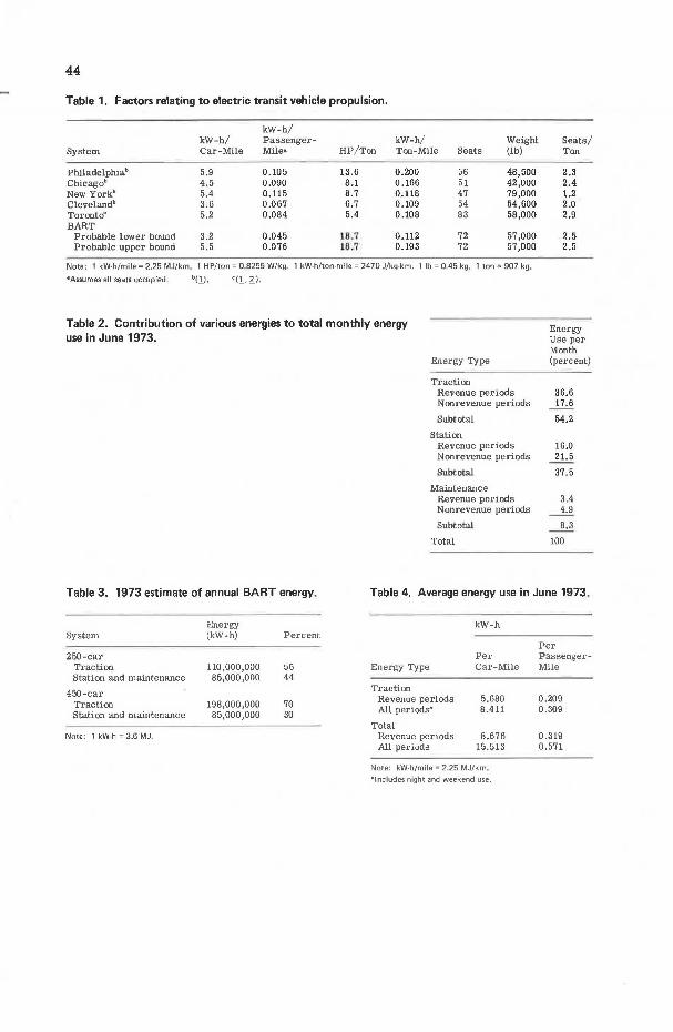
A survey of existing systems indicates an approximate energy demand range into which the BART system might fall. Table 1 gives the energy and power requirements of five such systems. For comparison purposes, the BART traction energy estimate is bracketed by a probable lower bound [3.2 kW-h/car-mile (7.2 MJ/km)J and a probable upper bound [5.5 kW-h/car-mile (12.4 MJ/km)J. These terms and their justification are discussed in detail later.

From Table 1, we can learn a number of things about what to expect from electric public transit systems. Unless radically new and different systems are proposed or

42

developed, we should be able to use the figures from Table 1 to make at least approx­imate estimates of power and energy use.

The energy demand per car-mile (kilometer) should be somewhere near 5 kW-h/car­mile (11.3 MJ/kmJ. A particularly light or streamlined car or one that makes relatively few stops or effectively uses regenerative braking should demand less energy. Opposite characteristics would lead to higher figures.

Table 1 also gives perhaps the most important factor for passenger systems, the energy demand per passenger-mile (kilometer), assuming that each seat is filled and there are no standees. This is an idealized condition. The dependence on percentage of seats occupied will be discussed in detail la ter in the paper. A value of 0.06 to 0.10 kW-h/passenger-mile (0.02 and 0.14 MJ/lon) should be reasonable for approximate planning purposes.

Electric motor power per tons (kilograms) of vehicle is an important factor because of its relation to the ability of the vehicle to accelerate . For example, the BART sys­tem has a maximum acceleration of 3 mph/sec (1.34 111/s/s). This is a high rate, close to the limit of comfort. Hence, BART vehicles require rather high-powered motors. Fast acceleration is necessary if a high average speed is to be maintained and stations are fairly close to each other. [BART has a peak speed of 80 mph (129 km/h) and an average design speed of 45 mph (72 km/h)].

Energy demand also depends on station spacing and aver age speed. Note the fairly strong correlation between traction power and traction energy (Table 1). Trains that make frequent stops and mai1ttain a high average speed must be high-powered and will consume more energy per ton-mile (kilogram-kilometer) than slower trains with less frequent stops. But trains that make frequent stops have a good potential for making effective use of regenerative braking.

From an energy use standpoint, it is desirable to keep the r atio of seat density per ton (kilogram) high. However, other factors, including safety and comfort of ride, tend to favor greater weight. The designer has a compromise to make here. The high ratio of seat density per ton (kilogram) for the BART system reflects, to some extent, the availability of new lighter and stronger vehicle construction materials and new de­sign techniques.

ENERGY USE BY BART

In that the BART system is not completely operational as yet, the data on actual energy being used by BART will certainly differ somewhat from final energy data. This might suggest that we should wait until the system is operating normally to obtain data. There are two reasons for proceeding at this time with only preliminary data. First, there is a need today for information about energy costs of transportation systems. Planning of future systems cannot wait for final, normal-operating data. Second, the process of evaluating the preliminary data with respect to weaknesses sheds light on the way in which energy is used in various ways in the system. This also provides a logical background for our discussion of load factor effects.

At least four factors operate to make the data incomplete as of July 1974: (a} BART is incomplete (not all tracks are in use), (b} more trains will be added, (c} the system is in a check-out period, and (d) the automatic control system is not fully operative.

The data for daily traction, operation, and maintenance energy used by BART during June 1973 were used as the basis for this analysis. we have reduced these raw data (2) in a number of ways to facilitate evaluation. In the following, we distinguish be­tWeen revenue periods, when the system carries passengers (5 a.m. to 8 p.m., Monday through Friday), and nonrevenue periods.

Table 2 gives the way in which the various energies contributed, on a percentage basis, to the total monthly energy use. The first observation from Table 2 is that the -

43

energy split between traction and station and maintenance is nearly 50-50 (early es­timates suggested a 40-60 split). Since station and maintenance energy is almost fixed (independent of traction mileage or passenger number s), an incr ease in car-miles (kilometers) will tend to cause an even greater percentage increase in traction energy. Hence, it is now anticipated that, when BART becomes fully operational, traction en­ergy will exceed that of operation and maintenance and perhaps will have a split greater than 60-40, the inverse of the original estimate. Table 3 gives a recent updated BART es timate of annual energy use based on early data (Figure 1).

If the current (1973) estimate is compared with the 1972 estimate, we find that the traction energy estimate is up by 22 percent and that station and maintenance energy estimates are down by 35 percent.

The estimation error in the case of station and maintenance energy is not difficult to understand. Little is known about these energy requirements. We are not aware of the availability of any station and maintenance statistics analogous to the national trac­tion statistics given in Table 1. The original estimates of station and maintenance en­ergy, made with few data, were conservative. We also observed that station energy is quite dependent in general on geographic and climatic factors, which determine heating, cooling, and lighting needs.

There is a dramatic increase in percentage of energy used for traction when 250 cars ar e compared with 450 cars (Table 3) . The reason is obvious: Fixed cos ts (station lighting, administration, escalators, maintenance facilities) when established change little, but traction ene,rgy goes up proportionately, as cars are added. The net effect is that the total ener gy per car-mile (kilometer ) goes down as car-miles (kilometers) go up. The more the system is used, the less it costs per unit of use.

Another inter esting set of data obtainable from the raw data is the current ener gy required per car-mile (kilometer) and passenger-mile (kilometer>. These data a re given in Table 4. These data are based on operating periods early in the life of the system. As system use increases s ubstantially, the energy cost per car-mile (kilo­meter) will decrease quite s ignificantly. This effect is discussed in some detail at the end of this section.

Why do nonrevenue periods tend to require so much energy? One might expect the system would be turned off during these periods. In fact, the system remains mostly turned on for 93 of 168 hours of the week when the system is not operating. The raw data show that the ratio of revenue period station and maintenance energy to total sta­tion and maintenance energy is nearly equal to the ratio of revenue hours to total hours in the week. Station lighting stays on for security and maintenance reasons. At least, partial parking lot lighting comes on or stays on at night. Other facilities remain ac­tivated for testing, security, and maintenance.

The traction energy demand during nonrevenue periods represents 17. 6 percent of all energy used by BART (Table 2). Nonrevenue period traction energy is used for ve­hicle testing and for lighting and heating or cooling vehicles not in service. Data from BART indicate an almost constant nonrevenue period power load of about 4 MW. Since this load is consistent 24 hours a day on Saturday and Sunday and during week nights, we deduced that little of it can be for testing. At this time, almost all cars are left in an energized mode with third-rail power on. Vehicles are heated and lighted, and some pumps are run continuously. This load per car is near 20 kW.

It is not entirely clear why cars are left hot while they are not in use. At least two factors contribute to this mode of operation. The air conditioner compressor pump­down cycle is 15 min. Apparently it would be necessary to have personnel monitor this process. In addition, during initial testing of vehicles, a number of problems were encountered that made it desirable to keep the vehicles hot. It is not clear at this time whether this mode is a permanent necessity or whether it can be phased out as the system approaches full operational status. It certainly seems reasonable that planners of future systems should ask design engineers whether live storage is actually necessary or desirable.

Traction energy is all the energy supplied to the 1,000-V de third rail. It supplies pure t r action or vehicle propulsion energy and auxiliar y energy for vehicles in oper­ation (heating, cooli.ng, lighting) and for stand-by vehi cles not in oper ation. The

44

Table 1. Factors relating to electric transit vehicle propulsion.

kW-h/ kW-h/ Passenger- kW-h/ Weight

System Car-Mile Mile a HP/Ton Ton-Mile Seats (lb)

Philadelphia' 5.9 0.105 13.6 0.200 56 48,500 Chicago' 4.5 0.090 8.1 0.166 51 42,000 New York' 5.4 0.115 8.7 0.118 47 79,000 Cleveland' 3.6 0.067 6.7 0.109 54 54,600 Torontoc 5.2 0.084 5.4 0.108 83 58,000 BART

Probable lower bound 3.2 0.045 18.~ 0.112 72 57,000 Probable upper bound 5.5 0.076 18.7 0.193 72 57 ,000

Note: 1 kW-h/mile = 2.25 MJ/km. 1 HP/ton= 0.8255 W/kg. 1 kW-h/ton-mile = 2470 J/kg-km. 1 lb= 0.45 kg. 1 ton= 907 kg. 8Assumes all seats occupied. b(.l). <::(L 2_) .

Table 2. Contribution of various energies to total monthly energy use in June 1973.

Energy Type

Traction Revenue periods Nonrevenue periods

Subtotal

Station Revenue periods Nonrevenue periods

Subtotal

Maintenance Revenue periods Nonrevenue periods

Subtotal

Total

Seats/ Ton

2.3 2.4 1.2 2.0 2.9

2.5 2.5

Energy Use per Month (percent)

36.6 17 .6

54.2

16.0 21.5

37.5

3.4 4.9

8.3

100

Table 3. 1973 estimate of annual BART energy. Table 4. Average energy use in June 1973.

Syste111

250-car Traction Station and maintenance

450-car Traction Station and maintenance

Note: 1 kW-h = 3.6 MJ.

Energy (kW-h)

110,000,000 85,000,000

198 ,000 ,000 85,000,000

Percent

56 44

70 30

kW-h

Per Energy Type Car-Mile

Traction Revenue periods 5.680 All periods• 8.411

Total Revenue periods 8.676 All periods 15.513

Note: kW-h/mile = 2.25 MJ/km. a Includes night and weekend use.

Per Passenger-Mile

0.209 0.309

0.319 0.571

45

stand-by vehicles are in live storage and draw about 20 kW in this condition. If auxil­iary ener gy for oper ating vehicles or for vehicles in live storage is discounted, then the 5.680- kW- h/car-mile (12 .78-MJ/km) value given in Table 4 decreases . If regener­ative braking is effective in returning energy to the system, net traction energy will be further reduced.

To quantify these effects, we first performed a calculation that eliminated the energy supplied to vehicles in live storage . This reduced traction energy to about 4. 5 kW-h/ car-mile (10.1 MJ /kmL Since auxiliary power demand fo r operating vehicles is about 20 kW and aver age t rain speed i s 45 mph (72 km/h), we assume an auxiliary energy de­mand of approximately 0. 5 kW-h/ca.r-mile (1.1 MJ/ k.m). Discount ing this demand further reduces tr action energy to about 4.0 kW-h/ car-mile (9 MJ/ km). Therefore, our best estimate is that the pure propulsion energy requirement of a BART vehicle, discounting auxiliary energy and possible regenerative energy return, is 4.0 kW-h/ ca.r­mile (9 MJ /km).

It is anticipated that some fraction of this pure propulsion energy can be recovered by the regenerative braking system. An energy return from regenerative braking of 20 percent is probably a reasonable upper bound. The degree of success of regenera­tive braking will not be clear until the BART system is fully operational.

From the discussion above, it is clear that three energy factors could increase or decrease the stated tr action energy based on the pure propulsion energy demand of 4.0 kW- h/ car-mile (9 MJ/km). These factors a re as follows (1 kW-h/ car - mile = 2.2 5 MJ/km):

Factor

Regenerative braking Auxiliary energy for

operating cars Auxiliary energy for

live storage

Energy Range (kW-h/ car-mile)

0.0 to 0.8

0.5

0.5 to 1.0

Effect

Energy saved Additional

energy used Additional

energy used

Hence, the traction energy can range from a probable lower bound of 3.2 kW-h/ car­mile (7.2 MJ/ km) to a p1·obable upper bound of 5.5 kW-h/ car- mile (12.4 MJ/km). The correct value to use depends on the assumptions the planner wishes to make and on the eventual degree of success of regenerative braking. If the planner or evaluator be­lieves that auxiliary energy for operating cars is a part of traction energy, then 0. 5 kW-h/ car-mile (1.1 MJ/ km) will be added. If the planner believes it is a convenience, analogous to the convenience of a station, then it may be accounted for another way, perhaps as an element of nonpropulsion operating costs. Of course, it must be ac­counted for eventually as some part of the total system energy.

The live storage factor is even more difficult to account for, and it may be possible to eventually eliminate live storage in the system. Or, if live storage is necessary, it may be desirable to account for it other than as an element of traction energy.

All of the above assumptions or accounting choices are necessarily left to the planner. For our analysis of passenger loading effects in the next section, we assume trac­

tion ener gy to be 5 kW-h/car-mile (11.3 MJ /km). For purposes of comparing BART with buses and automobiles, we consider both the probable upper bound and the probable lower bound.

Next we consider the relation of energy use to annual car-miles (kilometers). Table 4 shows the energy required by BART cars in June 1973. As time passes, this energy will decrease for a number of reasons. Fixed operation and maintenance costs will be averaged over more car-miles (kilometers) and the opportunity for regenerative braking will incr ease. The r elative amount of live s torage should also decrease. The result is a r oughly inverse (hyperbolic) rela tion of energy intensity to a1mual car-miles (kilo­meters). Some of the above factor s have been considered in a recent projection of future energy costs made by BART (~.

46

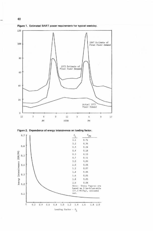
We are now in a po::;itiou to reconsider the power dernaud::; of BART. .r1gure i gives an es timate of _power demand based on the data available at this time. The base power demand of about 16 MW is required for stations and maintenance (8 MW) and for auxil­iary power to an assumed 400 operating and live storage cars. The peaks are estimated from anticipated train use when the system is fully operational. The major change in the 1973 estimate when compared with the 1967 estimate is that station and maintenance energy is somewhat less than had been originally estimated. In addition, the peak power demand is about 0.5 percent of the capacity of the area's power plant, the Pacific Gas and Electric Company.

A brief review of the way in which nonpropulsion energy is used for BART shows that, on the average, a BART car uses about 20 kW of power for nontraction purposes. About 1 kW is used in lighting, 10 kW for air conditioning, 20 kW for heating, and about 25 kW for other miscellaneous purposes such as fans, blowers, pumps, controls, and convenience outlets. Not all of these are on at the same time of course. The av­erage demand is about 20 kW.

EFFECTS OF VEHICLE LOADING ON ENERGY USE

Vehicle loading or the number of passengers on a vehicle affects energy use in two ways: It us ually has a small effect on the weight and, hence, the ener gy use per car­mile (kilometer), and it has a major effect on energy use per pas s enger-mile (kilo­meter). This latter measure is almost inversely proportional to the number of pas­sengers carried.

Effect of Passengers on Vehicle Weight

Before discussing the important problem of energy use per passenger-mile (kilometer), we must briefly consider the effect that passengers have on vehicle weight. The weight of a vehicle is

W = Wo + pWp

where

Wo =weight of the vehicle without passengers, p = number of passengers, fr =loading factor (fraction of seats with passengers), S = number of seats per vehicle, and

WP = average weight of passenger = 150 lb (68 kg).

(1)

(2)

For most motorized vehicles, fLSWP in equation 2 tends to be fairly small. In the case of BART, W0 "" 57,000 lb (25 855 kg) and S = 72. Therefore, equation 2 becomes approximately

w = 57,000 + 10,000 fr (3)

The loading factor can vary from 0 to about 2 (fL > 1 indicates standees). Hence, a BART vehicle with every seat occupied has a total weight of 19 percent greater than its zel'o-passenger weight . [A 4,000-lb (1 814- kg) automobile with 5 seats has almost

47

exactly the same percentage increase in weight, when fully loaded, as the BART vehicle.J

Effect of Loading on Energy Intensity

As we noted previously, passenger loading does not have a great effect on the weight of a vehicle. Hence, one approach to determining the effect of passenger loading on energy intensity in units of energy _per passenger-mile (kilometer) would be to assume the weight to be constant. For the time being, however, we will include the effect of loading on weight. We will assume there is a BART vehicle that requires 5 kW-h/car-mile (11.3 MJ/km) and that fL = 0 (no passengers>. We further assume that traction energy in­creases by a proportionality factor of 0.8 times the weight. (This means that about 20 percent of traction energy is not weight dependent. This includes aerodynamic drag, for example .) Based on the above assumptions, the energy required per car-mile (kilometer) is (CM = car-mile, PM = passenger-mile)

E - 5 x 57,000 + 8,000 fL CM - 57,000

The energy per passenger-mile (kilometer) is

E _ EcM PM -p

EcM = 72fL

= 7; (~ + 0.14)

- 0.07 0 01 - fr + .

(4)

(5)

It is clear from equation 5 that, for typical loading factors near 0.25, the effect of passenger weight (the second term in equation 5) is not very important. It does, how­ever, become quite important for load factors in the range from 1 to 2. Figure 2 shows the loading effect given by equation 5.

Loading Factor Versus Comfort and Convenience

Figure 2 shows the important relationship behveen energy cost per passenger-mile (kilometer) and passenger loading. It is clearly desirable from an energy standpoint to have as high a load factor as possible. However, two other important considerations argue against high load factors. The first is comfort. If fL > 1, some passengers are standing. If fL approaches two, the vehicle becomes crowded and even more uncom­fortable. This decreases the quality of the ride and will probably discourage some passenger use.

The second consideration is convenience. Passengers usually wish to wait as short a time as possible for a train. This means frequent train service and lower load fac­tors. It is not clear, however, that doubling the train frequency will halve the load factor. Doubling the train-frequency will probably result in a more attractive system, and the result will be that the new load factor should fall somewhere between the original

48

Figure 1. Estimated BART power requirements tor typical weekday.

i2a

iaa 1967 Estimate of Final Power lle!Mnd

8a

6a

4a

2a

a 12 3 6

AM

9 12

NOON

3 6

PM

9

Figure 2. Dependence of energy intensiveness on loading factor.

a. 7 l fL EPM

a.1 a. 71 a.2 a.36

a.6 a.3 a.24

~ a.4 a.18

...... o.s a.s a.is

~ a.7 a.11

"' a.9 a.a9 "' Q) a. 4 i.a 0.08 <=I ~ 1.2 0.07 ..... "' ~ 1.4 a.06

~ a. 3 1.6 a.as @ 1.8 a.as '" ~ a. 2 2.a o.a4

Note: These figures are based on 5 kw-h/car-mile (11.3 MJ/kg). unloaded

a.1

a a.2 a.4 0.6 a.8 1.0 1.2 1.4 1.6 1.8 z.a

Loading Factor - £1

12

49

load factor (before doubling the train frequency) and half that original load factor. We can generalize this relation by writing

where

kfLO fL.l =-f-

fL.o =original load factor, fLl =new load factor,

f = factor by which the frequency of trains is increased, and k =factor by which total ridership increases.

(6)

The factor k probably lies roughly between 1 and 2, depending on the increased at­tractiveness of the new system. We are essentially stopped at this point by a lack of knowledge about how k varies with f. Availability of such a relation would allow us to select a train frequency that maximizes fL.l and hence minimizes energy per passe nger­mile (kilometer). This may or may not, of course, be perceived as a desirable de­cision criterion. Eventually the conflicting goals of energy efficiency and comfort and convenience must be studied in more detail.

ENERGY COSTS OF BART CONSTRUCTION

Input-Output Analyses

The amount of energy consumed as a result of a given final demand placed on the economy must be determined. Let X be an n-dimension vector of total outputs of the economy, each element of which represents the value of output of a given sector. In particular, each element x1 is the output of sector i and consists of the sales to all other sectors in which the output of i is used as an intermediate good plus the sale of the output of i, which is used in final consumption. Symbolically,

n x1 = L a1JXJ + Y1 (7)

j=l

where

XJ = output of sector j, a1J =technical coefficient representing the amount of the i th output needed for pro­

duction of one unit of j th output, and Yi =amount of x1 used as final consumption.

If there are n sectors in the economy, then i can take any value from 1 to n and make a total of n equations in the form of equation 7. This set of equations may be repre­sented in matrix form as follows

X=AX+Y (8)

where Xis an n-dimension column vector of gross outputs; A is an n x n matrix of

50

input-output coefficients, the ij th element of which tells how much output of sector i is needed to produce one unit of output j; and Y is an n-dimensional column of final de­mands. A more interesting form of equation 8 to solve for gross output X as a function of final demand Y is

(9)

where I is an n x n identity matrix. This form of equation 9 is interesting because it tells us what gross output throughout the economy is required to sustain a final demand of Y. Using equation 9, we can determine what gross production l::i. Xis necessary to sustain a final demand l::i. Y, which is the construction of, for example, the BART system.

The task of determining tile energy content of the output has been undertaken by the Center for Advanced Computation (3) whose analysis follows. Take row i from A and denote it by ai. If i is an energy sector, for example, coal, then the tYPical element of (ai =au, ai2, ... , ai.), which is aq, represents the value of coal needed to support $1 of production of the j th output. If pi is the price of the i th output (coal), the (1/pi) a1 ='Yi gives the physical quantity of coal needed in production. Therefore, let

Yi = -, -, ... , - = Ya, ')'12, ... , 'Yin (au ai 2 a1•) ( ) Pi pi pi

(10)

Each Y!J gives the physical quantity of coal needed to sustain the output of $1 worth of the j th sector. Since the tYPica.l element of (I - A)-~ which we denote as AiJ, gives the value of production in sector i necessary to sustain fuial demand of $1 of output in sector j, we can proceed to interpret 'Y1(I - A)- 1 =ti. Each element of the row ti,

n tiJ = ~ YiJ AJ1, is the total physical amount of coal (output of energy sector i) needed

j=l by all sectors to sustain $1 of final demand in sector j.

Given that there are m energy sectors, there will also be m vectors of the type Yi or

R <= (11)

r.

where R is an m x n dimension matrix. Thus,

R(I - A)- 1 = T (12)

t.

where Tis an m x n matrix whose tYPical element tiJ gives the physical quantity of en­ergy sector i (coal, gas, oil) needed to sustain $1 of final demand in sector j.

To compute the amount of primary energy sources necessary to sustain Y, write

51

E =TY (13)

where E is an m x 1 dimensional vector of total quantities of energy sources required by the final demand Y. If Y1 represents the final demand placed on the economy by a transit system, then E1 = TY1 is the total quantity of energy sources required through­out the economy to sustain its production. It is easy to convert the quantities of coal and oil to any desired conventional energy unit such as Btu (J), and this is what the el­ements of E tell us.

There are some caveats in using the input-output approach in estimating energy use. The lag with which input-output matrices are published is very long. For example, the 1963 input-output matrix of the U.S. economy was published by the Bureau of Eco­nomic Analysis, U.S. Department of Commerce, in 1969. With this kind of lag time, the structure of the economy, in the sense of how much of what is needed to produce any given item, will have changed during the interim. If the 1963 matrix had been applied to energy problems when it first was published in 1969, there certainly would have been errors in the analysis. This is the problem that cannot be overcome.

As with any empirical work, the input-output matrix is sensitive to the conventions used in data collection. A change in conventions in gathering the data or in assigning or categorizing the output of a given subsector will change the input-output matrix and not cause a corresponding change in real structure of the economy.

The input -output matrix is built in value terms (prices times quantities). This means that some price level is used in its construction. Use of a different price level in calculating the value of final demand at a time other than the time the matrix was constructed will result in an error being introduced into the results. A correction for changing price levels must be included to eliminate this source of error; this is some­thing the user of input-output techniques can do.

Approximate Estimate of Energy Requirements of BART

An approximate estimate of the energy required by the vector of final demands given in Table 5 can be derived as follows. Take the total amount of energy consumed in the United States for a given year and divide that amount by the total final demand, or gross national product, of that year to get the average energy per dollar of final demand. In 1965 this figure was 78,800 Btu (83 million J) per dollar output (4). Then, simply multiply the total dollar final demand generated by BART by this-figure (5). (Because 1963 is close to 1965, the energy structure of the economy will not be too dissimilar at these dates.) From Table 5, the total classified by input-output sector as of the fall of 1972 is approximately $ 808 million. The total BART cost is more like $1.4 billion, but the balance has yet to be classified by input-output sector. For the purposes of this comparison, the smaller figure is used. By multiplying, we find that 63,649,360.4 MBtu (67 x 10L6 J) are required if each dollar used the energy that the average final demand dollar required.

Input-Output Estimate of the Energy Requirements of BART

If we take the T-matrix of equation 12j convert it to energy units instead of quantity of energy sources [i.e ., tons (kilograms of coal, gallons (liters) of oil], and finally sum T over its rows element by element, we get a row T** (3). Each element t'l'* gives the total amount of energy (both direct and indirect) in energy units [Btu (J) ] needed to sustain $1 in final dema nd in sector j. Taking the product of the row T** with the column Y (Table 5), we get

T**Y = 62,684,232.625 MBtu (66 x 1015 J) (14)

52

This estimate is within 1 million MBtu (1055 x 101 2 J) or 1.5 percent of the preliminary estimate us ing only the average ener gy intensity for 19 65.

If we extrapolate these r esults to the tot al anticipated capital cost of about $ 1.4 bil­lion for BART, we obtain a total capital energy cost of about 109 million MBtu (11 5 x 1015 J). The credibility of such an extrapolation is discussed later.

Next, we compare the energy required to build the system with the energy required to operate it. As s tated ear lier , BART currently anticipates arunial energy demand by a 450- car system to approximate the following : (a) 198 million kW-h/year (712 million MJ/ year) fo r traction, and (b) 85 million kW-h/year (306 million MJ/ year) for station and maintenance.

This is electric energy at the point of use. To estimate the thermal energy [in Btu (J)] into the power plant to provide this electric energy, we multiply by 10,000 Btu/ kW-h (2.93 J / J}. This accounts for thermal powe r plant i neffi ciencies and tr ansmission/ distribution losses. F\J.rthermore, to compare initial capital energy costs with operat­ing energy, we assume that the system operates for 50 year s and multip ly by this factor also. The total ener gy demand over the 50-year assumed lifespan is given in Table 6.

Thus, we see that, with the assumptions made her e, traction ener gy is about 40 per­cent of the total energy used by BART. In comparis on Hirs t (5) has found U1at 50 per­cent of the energy used in building and operating automobiles each year is propulsion energy from gasoline.

Evaluation of Input- Output Results

We now evaluate the extraordinary agreement between the construction energy costs obtained by the approximate method and those obtained by the input-output approach. In view of the assumptions made in both methods, the level of agreement is surprising. The obvious question is whether this is mere chance or whether the approximate method is actually highly accurate for this type of system. If the latter is true, then the analysis is simplified considerably. Unfortunately, the scope of this study does not permit the necessary in-depth evaluation required to answer this question.

A related question is whether it is accurate to extrapolate from the $808 million data to an energy figure for $1.4 billion as we did in the previous section. The answer is yes if the $808 million worth of work is representative of the energy intensiveness of the entire project. We do not have the data to answer this question; therefore, the re­sults in the previous section may be slightly erroneous.

BART IMPACT ENERGY

BART impact energy is used in building and operating systems related to BART or that e:xist because BART exists. This includes new office buildings constructed along BART corridors because of the convenience of BART. It also includes, on the negative side, the decrease in energy because of a shift from existing automobiles and buses to BART, and, on the positive side, the generation of new trips by new business and in­dustry generated by BART. rt is sometimes thought that BART will lead to less cars on the bridges or result in a net savings of energy. Probably neither of these as­su mptions is correct. BAR T' s impact on the co1mnu1lity in s timulating gr owth may well add more automobile trips than it replaces and lead to a net increase in energy use. This should not be construed as inferring that BART is thus a failure . 011 the contrary, it might be interpreted as evidence that BART has succeeded in stimulating the economy of the region, including some urban areas that might otherwise have de­teriorated significantly.

Unfortunately, a detailed analysis of impact energy would be quite complex and well beyond the scope of this study. It may be that the Metropolitan Transportation Com­mission's BART impact study will provide sufficient data to carry out a partial energy impact study sometime in the future. Such a study would make use of trip replacement

53

and generation studies and new building costs, within the approach used in the previous section.

COMPARING BART WITH OTHER SYSTEMS

In this section, the energy demands of BART are compared with other systems, spe­cifically buses and automobiles. A decision must be made at the outset about what components of energy cost will be compared. To compare only propulsion (or traction) costs is somewhat limited and perhaps misleading. However, the inclusion of factors such as operation, maintenance, and construction costs makes the analysis more com­plex and speculative. For example, although construction energy for BART can be estimated, how does one estimate energy used to build the freeways, roads, parking lots, garages, and driveways required by buses and automobiles? Two comparisons are made, and a series of assumptions is made in each case. First, propulsion en­ergies only are compared. Then total energies are compared.

For BART traction energy, we use the probable upper and lower bounds introduced earlier in the paper. we assume a load factor of 25 percent or 18 passengers per ve­hicle and an energy conversion heat rate of 10,000 Btu/kW-h (2.93 J/J) (corres1Jonding to a p0wer plant/distribution system efficiency of 34 percent). For buses we assume 5 miles/gal (2 km/liter), a gasoline conversion rate of 136,000 Btu/gal (3.7x 10 7 J/ liter), a 50-seat vehicle, and a load factor of 25 percent or 12.5 passengers/vehicle. For the automobile we assume 12 miles/gal (5 km/liter), 136,000 Btu/gal (3. 7 x 10 7

J/liter, and 1.4 passengers per vehicle. The resulting propulsion energy intensities are given in Table 7 on a passenger-mile (kilometer) basis.

A number of facts should be kept in mind. First, the loading factors are assumed somewhat arbitrarily, although they tend to approximate national averages. Different loading factors could drastically change these comparisons. A fully loaded automobile (car pool) could be about as efficient as BART or a bus that is 25 percent loaded. How­ever, a fully loaded bus or BART with standees could be as much as 10 to 15 times more energy efficient than the average automobile. The great sensitivity of er.ergy comparisons to loading should be kept in mind at all times in transportation energy studies. ·

A second important fact is that, even though we have referred propulsion energy to power plant input energy, it is not obvious that the resulting comparison is completely fair. The energy source for the power plant could, in general, be coal, oil, natural gas, uranium, or hydroelectric power, each with different processing energy require­ments. Gasoline must also be processed in a refinery and is about 85 percent efficient. Hence, comparing fuel energies at the input to the power plant with energy into the auto­mobile has some real limitations.

Finally, we consider the question of comparative total energy use. As stated pre­viously, in the case of BART and automobiles, propulsion energy tends to be about 50 percent of total energy. Although these data are probably fairly accurate for automo­biles, BART must reach completion and experience some months of normal operation before comparative total energy use can be tested for BART. A similar analysis has not been made for buses. If buses have about the same 50-50 energy split and if the data for BART and automobiles are reasonably accurate, then we can obtain an esti­mate of total energy comparison by simply doubling the propulsion energy figures given in Table 7. This is fine for buses and automobiles but is ambiguous in the case of BART since we have two bounds. The traction estimates used previously assume that auxiliary energy is accounted for as traction energy and that regenerative braking is partially successful. On the basis of these assumptions, we assume a traction energy of 4. 7 kW-h/car-mile (10. 7 MJ/km) for purposes of calculating total BART energy.

Again, the reader must be cautioned that these results are based on some major as­sumptions: The extensive use of light, compact automobiles could reduce automobile energy use by more than two times; the allotment of energy costs to roads and garages is quite arbitrary; and the impact energy for BART and for other vehicles has not been considered quantitatively.

54

Tablii 5. c:. , .. I .1.-. ................. 1 .... 1,. ......... 1 ,.... ,.,, +I,,.., 11 C ,..,..,... ... ,..."""' /i"'"'11+."'11+ft11+ I 11101 UOlllUllU tJIU"'""'"' VII ur"' - ........................... , ''"'I" .............. t" ... ..

sector) by energy requirements of BART.

Bureau of Bureau of Economic Economic Analysis Analysis Input-Output Final Demand Input-Output Final Demand Sector (current dollars)• Sector (current dollars)•

400 2,690,000 5303 3,477,000 1102 139,259,000 5308 10,319,000 1103 46,000 5502 30,000 1104 88,983,000 5603 798,000 1105 487,923,000 5604 197,000 1202 3,357,000 5703 84,000 2008 132,000 5805 231,000 3611 2,657,000 5903 9,000 3808 8,551,000 6104 20,304,000 4004 27,475,000 6411 314,000 4102 14,000 6412 179,000 4203 50,000 6600 2,000 4601 5,723,000 6801 23,000 4704 275,000 6802 1,000 4901 76,000 6803 134,000 4903 795,000 7303 5 000 4907 2, 786,000 Total 807,733,000 5201 834,000

•These expenditures occurred over a 20·year period. Expenditures in the same sector that occurred at different times are lumped into the sector total and are not corrected for price in· creases. Thus, the sector totals are not, for example, in 1963 constant dollars.

Table 6. Total BART energy requirements.

Table 7. Comparative propulsion energies.

Btu Propulsion Total Energy Type (x 1012

) Percent Energy (Btu/ Energy (Btu/ passenger- passenger-

Construction 110 44 Vehicle mile) mile) Traction 100 40 Operation and BART

maintenance 40 16 Probable lower bound 1,800 5,200

Total required 250 Probable upper bound 3,600 Bus 2,200 4,400

Note: 1 Btu= 1055 J. Automobile 8,100 16,200

Note: 1 Btu/passenger-mile== 659 J/km.

55

Based on the assumptions made here, we conclude that there are not sufficient data to favor BART over buses or vice versa on an energy basis, but that both BART and buses are more energy efficient than the automobile.

CONCLUSIONS AND IMPLICATIONS

1. BART traction energy will range from 3.2 to 5.5 kW-h/ car-mile (7.2 to 12.4 MJ/ km), depending on how certain auxiliar y energies are accounted for and on the degree of success of the regenerative braking system. The additional energy per car-mile (kilometer) resulting from system operation and maintenance should range from about 1.0 to 1.5 kW-h/ car-mile (2 .3 to 3.4 MJ/km) when the system is fully operational.

2. BART is in a transition or break-in stage at this time. Although final energy levels can be estimated, these should be checked from real data when BART is fully operational.

3. BART traction energy, as with any system, is highly sensitive to load factors . Traction energy per passenger - mile (kilometer) is almost inver sely proportional to the number of passengers.

4. If the BART system is used for 50 years, the energy required for propulsion will be roughly 40 percent of total energy. The other 60 percent is for construction and operation and maintenance.

5. The approximate method used to find construction energy and the complex input­output approach yield almost exactly the same result. This is surprising, considering the assumptions that must be made in both cases. Some attempt should be made to de­termine if this relation is consistent.

6. Although it is believed that impact energy is significant, no attempt is made here to quantify it. The Metropolitan Transportation Commission's BART impact study may greatly facilitate this analysis.

7. A comparison of BART with buses and automobiles suggests that the propulsion energy and total energy demand of both buses and BART are about 2 to 3 times lower than that for automobiles (assuming an average size car and a loading factor of about 25 percent for all vehicles). Such comparisons are highly sensitive to the assumptions made.

On an energy basis, BART is more efficient than automobiles but not necessarily more efficient than buses . A number of steps could be taken in private or public transit to reduce energy use. More detailed data should be obtained on BART and other new systems as they become operational. Construction energy and impact energy are sig­nificant but have not as yet been studied in sufficient detail to provide conclusive results . Comparing energy costs of transportation systems depends on the nature of the systems and the assumptions made about their operation.

ACKNOWLEDGMENT

This paper is based on a study performed in cooperation with Business and Transporta­tion Agency, California Department of Transportation. The contents of this report reflect the views of the authors, who are responsible for the facts and the accuracy of the data presented. The contents do not necessarily reflect the official views or policies of the state of California. This report does not constitute a standard, specifi­cation, or regulation.

REFERENCES

1. A. Lang and R. Soberman. Urban Rail Transit: Its Economics and Technology. M.I. T. Press, Cambridge, Mass., 1964.

56

2. rr. j. Healy. Energy Requ1ren1ents of the Bay Arca Ra.pid Transit (BART) Systen1. California Department of Transportation, Santa Clara, Nov. 28, 1973.

3. R. A. Herendeen. An Energy Input-Output Matrix for the United States 1963: User's Guide. Center for Advanced Computation, Univ. of Illinois, Urbana, Document 69, 1973.

4. T. J. Healy. Energy Costs of an Electric Mass Transit System. Graduate School of Engineering, Univ. of Santa Clara, 1972.

5. E. Hirst. Energy Consumption for Transportation in the U.S. Oak Ridge National Laboratory, Oak Ridge, Tenn., ORNL-NSF-EP-15, March 1972.