Institut de Recerca en Economia Aplicada Regional i Pública Document de Treball 2013/21, 23 pàg. Research Institute of Applied Economics Working Paper 2013/21, 23 pag.

Grup de Recerca Anàlisi Quantitativa Regional Document de Treball 2013/13 23 pàg.

Regional Quantitative Analysis Research Group Working Paper 2013/13, 23 pag.

“Tourism demand forecasting with different neuralnetworks models”

Oscar Claveria, Enric Monte and Salvador Torra

Research Institute of Applied Economics Working Paper 2013/21, pàg. 2 Regional Quantitative Analysis Research Group Working Paper 2013/13, pag. 2

2

WEBSITE: www.ub-irea.com • CONTACT: irea@ub.edu

WEBSITE: www.ub.edu/aqr/ • CONTACT: aqr@ub.edu

Universitat de Barcelona Av. Diagonal, 690 • 08034 Barcelona

The Research Institute of Applied Economics (IREA) in Barcelona was founded in 2005, as a research institute in applied economics. Three consolidated research groups make up the institute: AQR, RISK and GiM, and a large number of members are involved in the Institute. IREA focuses on four priority lines of investigation: (i) the quantitative study of regional and urban economic activity and analysis of regional and local economic policies, (ii) study of public economic activity in markets, particularly in the fields of empirical evaluation of privatization, the regulation and competition in the markets of public services using state of industrial economy, (iii) risk analysis in finance and insurance, and (iv) the development of micro and macro econometrics applied for the analysis of economic activity, particularly for quantitative evaluation of public policies.

IREA Working Papers often represent preliminary work and are circulated to encourage discussion. Citation of such a paper should account for its provisional character. For that reason, IREA Working Papers may not be reproduced or distributed without the written consent of the author. A revised version may be available directly from the author.

Any opinions expressed here are those of the author(s) and not those of IREA. Research published in this series may include views on policy, but the institute itself takes no institutional policy positions.

Research Institute of Applied Economics Working Paper 2013/21, pàg. 3 Regional Quantitative Analysis Research Group Working Paper 2013/13, pag. 3

3

Abstract

This paper aims to compare the performance of different Artificial Neural Networks techniques for tourist demand forecasting. We test the forecasting accuracy of three different types of architectures: a multi-layer perceptron, a radial basis function and an Elman network. We also evaluate the effect of the memory by repeating the experiment assuming different topologies regarding the number of lags introduced. We used tourist arrivals from all the different countries of origin to Catalonia from 2001 to 2012. We find that multi-layer perceptron and radial basis function models outperform Elman networks, being the radial basis function architecture the one providing the best forecasts when no additional lags are incorporated. These results indicate the potential existence of instabilities when using dynamic networks for forecasting purposes. We also find that for higher memories, the forecasting performance obtained for longer horizons improves, suggesting the importance of increasing the dimensionality for long term forecasting.

Keywords: tourism demand; forecasting; artificial neural networks; multi-layer perceptron; radial basis function; Elman networks; Catalonia

JEL classification: L83; C53; C45; R11

Oscar Claveria. AQR Research Group-IREA. Department of Econometrics. University of Barcelona, Av. Diagonal 690, 08034 Barcelona, Spain. E-mail: oclaveria@ub.edu Enric Monte. Department of Signal Theory and Communications, Polytechnic University of Catalunya (UPC). Salvador Torra. AQR Research Group-IREA. Department of Econometrics. University of Barcelona, Av. Diagonal 690, 08034 Barcelona, Spain. E-mail: storra@ub.edu ���� Acknowledgements We wish to thank Núria Caballé at the Observatori de Turisme de Catalunya for providing us with the data used in the study.

2

1. Introduction

There has been a growing interest in tourism demand forecasting over the past

decades. Some of the reasons for this increase are the constant growth of world tourism,

the availability of more advanced forecasting techniques and the requirement for more

accurate forecasts of tourism demand at the destination level. Catalonia (Spain) is one of

the world’s major tourist destinations. More than 15 million foreign visitors came to

Catalonia in 2012, a 3.7% rise with respect to the previous year. Tourism accounts for

12% of GDP and provides employment for 15% of the working population in Catalonia.

Therefore, accurate forecasts of tourism volume at the destination level play a major

role in tourism planning as they enable destinations to predict infrastructure

development needs. The last couple of decades have seen many studies of international

tourism demand forecasting, but due to the insufficient databases available few studies

have been undertaken at a regional level.

Despite the consensus on the need to develop more accurate forecasts and the

recognition of their corresponding benefits, there is no one model that stands out in

terms of forecasting accuracy (Song and Li, 2008; Witt and Witt, 1995). Following

Coshall and Charlesworth (2010), studies of tourism demand forecasting can be divided

into causal econometric models and non-causal time series models. Nevertheless, there

has been an increasing interest in Artificial Neural Networks (ANN) due to

controversial issues related to how to model the seasonal and trend components in time

series and the limitations of linear methods. ANN have been applied in the many fields,

but only recently to tourism demand forecasting (Kon and Turner, 2005; Palmer et al,

2006; Chen, 2011, Teixeira and Fernandes, 2012).

Neural networks can be divided into three types regarding their learning strategies:

supervised learning, non-supervised learning and associative learning. The neuronal

network architecture most widely used in tourism demand forecasting is the multi-layer

perceptron (MLP) method based on supervised learning (Pattie and Snyder, 1996;

Fernando et al, 1999; Uysal and El Roubi, 1999; Law, 1998, 2000, 2001; Law and Au,

1999, Burger et al, 2001; Tsaur et al, 2002; Claveria et al, 2014). MLP neural networks

consist of different layers of neurons (linear combiners followed by a sigmoid non

linearity) with a layered connectivity.

3

An alternative approach is the radial basis function (RBF) architecture. RBF

networks consist of a linear combination of radial basis functions such as kernels

centred at a set of centroids with a given spread. Lin et al (2013) have recently

compared the forecast accuracy of RBF networks to that of MLP and Support Vector

Regression (SVR) networks. In MLP and RBF networks information about the context

is introduced into the input vector by the concatenation of several observation vectors.

In this study the context is composed of past values of the time series.

Whilst MLP neural networks are increasingly used with forecasting purposes, other

more computationally expensive architectures such as the Elman neural network have

been scarcely used in tourism demand forecasting. Elman networks are a special

architecture of the class of recurrent neural networks (RNN). The topology of Elman

networks follows that of a MLP network with feedback from the hidden layer neuron’s

activation. The Elman architecture takes into account the temporal structure of the time

series by means of a feedback of the activations of the hidden layer. Cho (2003) used

the Elman architecture to predict the number of arrivals from different countries to

Hong Kong.

As it can be seen, in spite of the increasing interest in machine learning methods for

time series forecasting, very few studies compare the accuracy of different neural

networks architectures for tourism demand forecasting. Additionally, the scarce

information available at a regional level, results in a very limited number of published

articles which make use of such data. This led us to compare the forecasting

performance of three different artificial neural networks architectures (MLP, RBF and

Elman) to predict inbound international tourism demand to Catalonia.

We used pre-processed official statistical data of arrivals to Catalonia from the

different countries of origin. Several measures of forecast accuracy and the Diebold-

Mariano test for significant differences between each two competing series are

computed for different forecast horizons (1, 3 and 6 months) in order to assess the value

of the different models. We repeated the experiment assuming different topologies

regarding the memory values so as to evaluate the effect of the memory on the

forecasting results. The memory denotes the number of lags used for concatenation

when running the models.

The structure of the paper is as follows. Section 2 briefly describes each type of

networks used in the analysis. The data set is described in Section 3. In Section 4 results

of the forecasting competition are discussed. Concluding remarks are given in Section 5.

4

2. Methodology

The use of Artificial Neural Networks for time series forecasting has aroused great

interest in the past two decades. One of the features for which neural-based forecasting

is increasingly applied is that ANN are universal function approximators capable of

mapping any linear or nonlinear function under certain conditions. As opposed to time

series linear models, and due to their flexibility, ANN models lack a standard systematic

procedure for model building. The specification of the model is based on the knowledge

of the problem at hand. Obtaining a reliable neural model involves selecting a large

number of parameters experimentally and require cross-validation techniques (Bishop,

1995). Zhang et al (1998) reviewed the main ANN modelling issues: the network

architecture (determining the number of input nodes, hidden layers, hidden nodes and

output nodes), the activation function, the training algorithm, the training sample and

the test sample, as well as the performance measures.

ANN models have three learning methods: supervised learning, non-supervised

learning and associative learning. Depending on the way in which the different layers

are linked, networks can also be classified as: feed forward, cascade forward, radial and

recurrent. The neuronal network model most widely used in time series forecasting is

the multi-layer perceptron method, which is based on supervised learning. To a lesser

extent, radial basis function and Elman neural networks are increasingly used for

forecasting purposes.

In this section we present the three neural networks architectures used in the study:

the multi-layer perceptron network, the radial basis function network and the Elman

network.

2.1. Multi-layer perceptron (MLP) neural network

The multi-layer perceptron architecture is the neuronal network model most

frequently used in time series forecasting. The MLP is a supervised neural network that

uses as a building block a simple perceptron model. The topology consists of layers of

parallel perceptrons, with connections between layers that include optimal connections

that either skip a layer or introduce a certain kind of feedback. As described in Cybenko

(1989), a network with one hidden layer can approximate a wide class of functions as

5

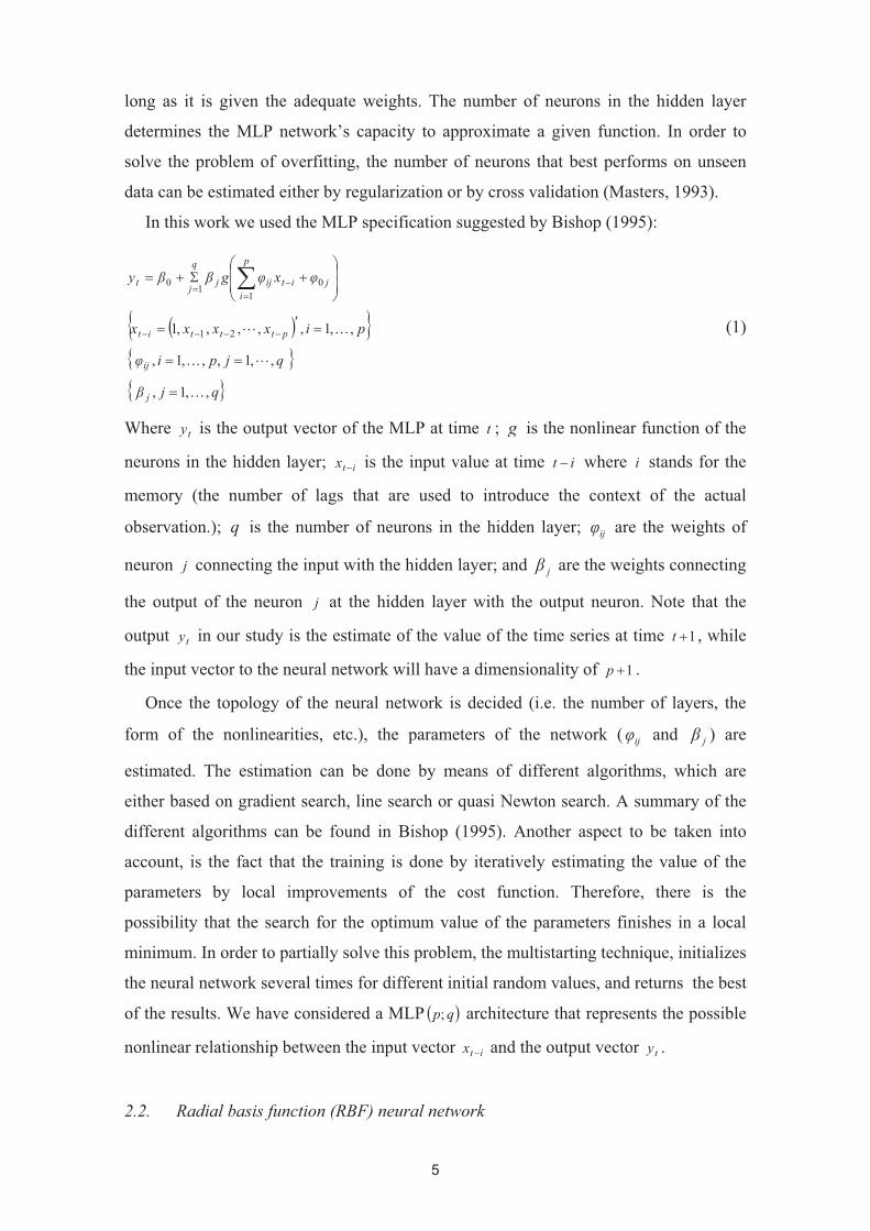
long as it is given the adequate weights. The number of neurons in the hidden layer

determines the MLP network’s capacity to approximate a given function. In order to

solve the problem of overfitting, the number of neurons that best performs on unseen

data can be estimated either by regularization or by cross validation (Masters, 1993).

In this work we used the MLP specification suggested by Bishop (1995):

� �� �� �� �qj�

qjpi�

pixxxx

�x�g��y

j

ij

ptttit

j

p

iitijj

q

jt

,,1,

,,1,,,1,

,,1,,,,,1 21

01

10

�

��

��

�

��

���

��

��

�

����

����

��

� �

(1)

Where ty is the output vector of the MLP at time t ; g is the nonlinear function of the

neurons in the hidden layer; itx � is the input value at time it � where i stands for the

memory (the number of lags that are used to introduce the context of the actual

observation.); q is the number of neurons in the hidden layer; ij� are the weights of

neuron j connecting the input with the hidden layer; and j� are the weights connecting

the output of the neuron j at the hidden layer with the output neuron. Note that the

output ty in our study is the estimate of the value of the time series at time 1�t , while

the input vector to the neural network will have a dimensionality of 1�p .

Once the topology of the neural network is decided (i.e. the number of layers, the

form of the nonlinearities, etc.), the parameters of the network ( ij� and j� ) are

estimated. The estimation can be done by means of different algorithms, which are

either based on gradient search, line search or quasi Newton search. A summary of the

different algorithms can be found in Bishop (1995). Another aspect to be taken into

account, is the fact that the training is done by iteratively estimating the value of the

parameters by local improvements of the cost function. Therefore, there is the

possibility that the search for the optimum value of the parameters finishes in a local

minimum. In order to partially solve this problem, the multistarting technique, initializes

the neural network several times for different initial random values, and returns the best

of the results. We have considered a MLP � �qp; architecture that represents the possible

nonlinear relationship between the input vector itx � and the output vector ty .

2.2. Radial basis function (RBF) neural network

6

The radial basis function neural network was first formulated by Broomhead and

Lowe (1988). RBF networks consist of a linear combination of radial basis functions

such as kernels centred at a set of centroids with a given spread that controls the volume

of the input space represented by a neuron (Bishop, 1995; Haykin, 1999). RBF

networks typically include three layers: an input layer; a hidden layer, which consists of

a set of neurons, each of them computing a symmetric radial function; and an output

layer that consists of a set of neurons, one for each given output, linearly combining the

outputs of the hidden layer. The input can be modelled as a feature vector of real

numbers, and the hidden layer is formed by a set of radial functions centred each at a

centroid j� . The output of the network is a scalar function of the output vector of the

hidden layer. The equations that describe the input/output relationship of the RBF are:

� �

� �� �

� �� �� �qj�

pixxxx

�

�x

xg

xg��y

j

ptttit

j

p

jjit

itj

itjj

q

jt

,,1,

,,1,,,,,1

2exp

21

21

2

10

�

��

�

���

������

������

�

�

��

���

����

��

�

��

�(2)

Where ty is the output vector of the RBF at time t ; j� are the weights connecting the

output of the neuron j at the hidden layer with the output neuron; q is the number of

neurons in the hidden layer; jg is the activation function, which usually has a Gaussian

shape; itx � is the input value at time it � where i stands for the memory (the number of

lags that are used to introduce the context of the actual observation); j� is the centroid

vector for neuron j ; and the spread j� is a scalar that measures the width over the input

space of the Gaussian function and it can be defined as the area of influence of neuron

j in the space of the inputs. Note that the output ty in our study is the estimate of the

value of the time series at time 1�t , while the input vector to the neural network will

have a dimensionality of 1�p .

In order to assure a correct performance, before the training phase the number of

centroids and the spread of each centroids have to be selected. The selection of the

number of hidden nodes must take into account the trade-off between the error in the

7

training set and the generalization capacity, which indicates the performance over

samples not used in the training phase. In the limit case, assigning a centroid to each

input vector and using a spread j� of high value would yield a look up table that would

have a low performance on unseen data. That means that the value of the exponential is

such that the output of the neuron is high for a distance between the observation and the

centroid equal to zero, and the output is zero when the distance is different from zero.

Therefore, the centroids and the spread of each neuron should be selected so that the

performance on unseen data is acceptable.

There are different methods for the estimation of the number of centroids and the

spread of the network. A complete summary can be found in Haykin (1999). In this

study the training was done by adding the centroids iteratively with the spread

parameter j� fixed. Then a regularized linear regression was estimated to compute the

connections between the hidden and the output layer. Finally, the performance of the

network was computed on the validation data set. This process was repeated until the

performance on the validation database ceased to decrease. The spread j� is a

hyperparameter, in the sense that it is selected before determining the topology of the

network, and it is tuned outside the training phase. Although a different value of j�

could be selected for each neuron j , usually a common value is used for all the

neurons.

2.3. Elman neural network

The Elman network, which is a special architecture of the class of recurrent neural

networks, it was first proposed by Elman (1990). The architecture is based on a three-

layer network with the addition of a set of context units that allow feedback on the

internal activation of the network. There are connections from the hidden layer to these

context units fixed with a weight of one. At each time step, the input is propagated in a

standard feed-forward fashion. The fixed back connections result in the context units

always maintaining a copy of the previous values of the hidden units. Thus the network

can maintain a sort of state of the past decisions made by the hidden units, allowing it to

perform such tasks as sequence-prediction that are beyond the power of a standard

multilayer perceptron.

The Elman architecture is a type of recurrent neural network. The output of the

network is then a scalar function of the output vector of the hidden layer:

8

� �� �� �� �� �qjpi�

qj�

qjpi�

pixxxx

z��x�gz

z��y

ij

j

ij

ptttit

tjijj

p

iitijtj

tjj

q

jt

,,1,,,1,

,,1,

,,1,,,1,

,,1,,,,,1 21

1,01

,

,10

��

�

��

��

��

�

��

���

��

��

�

���

���

����

��

�

�

�(3)

Where ty is the output vector of the Elman network at time t ; tjz , is the output of the

hidden layer neuron j at the moment t ; g is the nonlinear function of the neurons in

the hidden layer; itx � is the input value at time it � where i stands for the memory (the

number of lags that are used to introduce the context of the actual observation); ij� are

the weights of neuron j connecting the input with the hidden layer; q is the number of

neurons in the hidden layer; j� are the weights of neuron j that link the hidden layer

with the output; and ij� are the weights that correspond to the output layer and connect

the activation at moment t . Note that the output ty in our study is the estimate of the

value of the time series at time 1�t , while the input vector to the neural network will

have a dimensionality of 1�p .

The parameters of the Elman neural network are estimated by minimizing an error

cost function. In order to minimize total error, gradient descent is used to change each

weight in proportion to its derivative with respect to the error, provided the nonlinear

activation functions are differentiable. A major problem with gradient descent for

standard RNN architectures is that error gradients vanish exponentially quickly with the

size of the time lag between important events. RNN may behave chaotically, due to the

fact that there is a feedback, followed by a set of sigmoid nonlinearities, and as the sign

of the feedback loop is controlled by the learning algorithm, the algorithm may develop

an oscillating behaviour, unrelated to the objective function, and the value of the

weights may diverge. In such cases, dynamical systems theory may be used for analysis.

Most RNN present scaling issues. In particular, RNN cannot be easily trained for large

numbers of neuron units nor for large numbers of inputs units. Successful training has

been mostly in time series with few inputs.

There are different strategies for estimating the parameters of the Elman neural

network. Various methods for doing so were developed by Werbos (1988), Pearlmutter

9

(1989) and Schmidhuber (1989). The standard method is called backpropagation

through time, and is a generalization of back-propagation for feed-forward networks. A

more computationally expensive online variant is called real-time recurrent learning,

which is an instance of automatic differentiation in the forward accumulation mode with

stacked tangent vectors. In this paper, the training of the network was done by

backpropagation through time.

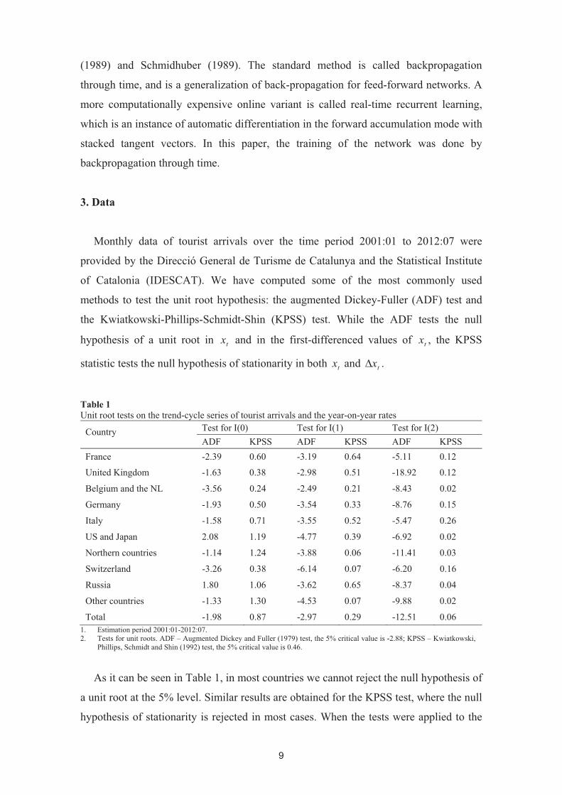
3. Data

Monthly data of tourist arrivals over the time period 2001:01 to 2012:07 were

provided by the Direcció General de Turisme de Catalunya and the Statistical Institute

of Catalonia (IDESCAT). We have computed some of the most commonly used

methods to test the unit root hypothesis: the augmented Dickey-Fuller (ADF) test and

the Kwiatkowski-Phillips-Schmidt-Shin (KPSS) test. While the ADF tests the null

hypothesis of a unit root in tx and in the first-differenced values of tx , the KPSS

statistic tests the null hypothesis of stationarity in both tx and tx� .

Table 1 Unit root tests on the trend-cycle series of tourist arrivals and the year-on-year rates

Country Test for I(0) Test for I(1) Test for I(2) ADF KPSS ADF KPSS ADF KPSS

France -2.39 0.60 -3.19 0.64 -5.11 0.12

United Kingdom -1.63 0.38 -2.98 0.51 -18.92 0.12

Belgium and the NL -3.56 0.24 -2.49 0.21 -8.43 0.02

Germany -1.93 0.50 -3.54 0.33 -8.76 0.15

Italy -1.58 0.71 -3.55 0.52 -5.47 0.26

US and Japan 2.08 1.19 -4.77 0.39 -6.92 0.02

Northern countries -1.14 1.24 -3.88 0.06 -11.41 0.03

Switzerland -3.26 0.38 -6.14 0.07 -6.20 0.16

Russia 1.80 1.06 -3.62 0.65 -8.37 0.04

Other countries -1.33 1.30 -4.53 0.07 -9.88 0.02

Total -1.98 0.87 -2.97 0.29 -12.51 0.06 1. Estimation period 2001:01-2012:07. 2. Tests for unit roots. ADF – Augmented Dickey and Fuller (1979) test, the 5% critical value is -2.88; KPSS – Kwiatkowski,

Phillips, Schmidt and Shin (1992) test, the 5% critical value is 0.46.

As it can be seen in Table 1, in most countries we cannot reject the null hypothesis of

a unit root at the 5% level. Similar results are obtained for the KPSS test, where the null

hypothesis of stationarity is rejected in most cases. When the tests were applied to the

10

first difference of individual time series, the null of non-stationarity is strongly rejected

in most cases. In the case of the KPSS test, we cannot reject the null hypothesis of

stationarity at the 5% level in any country. These results imply that differencing is

required in most cases and prove the importance of deseasonalizing and detrending

tourism demand data before modelling and forecasting.

In order to eliminate both linear trends as well as seasonality we used the year-on-

year rates of the trend-cycle component of the series. These series were obtained using

Seats/Tramo. Table 2 shows a descriptive analysis of year-on-year rates of the trend-

cycle series between January 2002 and July 2012. During this period, Russia and the

Northern countries experienced the highest growth in tourist arrivals. Russia is also the

country that presents the highest dispersion in growth rates, while France shows the

highest levels of Skewness and Kurtosis.

Table 2 Descriptive analysis of the year-on-year rates of the trend-cycle series

Country Tourist arrivals Mean SD Skew. Kurt.

France 5.06 13.69 2.13 8.93

United Kingdom 1.94 15.00 0.70 3.51

Belgium and NL 1.85 8.50 0.76 3.13

Germany 0.45 7.85 0.14 3.13

Italy 5.48 14.58 0.88 3.39

US and Japan 4.77 11.14 -0.08 2.64

Northern countries 8.24 16.97 0.25 2.70

Switzerland -0.21 9.86 0.28 4.93

Russia 16.06 32.12 -0.35 2.69

Other countries 6.90 10.02 -0.15 2.48

Total 3.75 7.04 -0.75 3.04 1. SD – Standard Deviation, Skew. – Skewness, Kurt. – Kurtosis

4. Results

In this section we compared the forecasting performance of three different artificial

neural networks architectures (multi-layer perceptron, radial basis function and Elman

recursive neural networks) to predict arrivals to Catalonia from the different visitor

countries. Following Bishop (1995) and Ripley (1996), we divided the collected data

into three sets: training, validation and test sets. This division is done in order to asses

the performance of the network on unseen data. The assessment is undertaken during

11

the training process by means of the validation set, which is used in order to determine

the epocs and the topology of the network. The initial size of the training set was

determined to cover a five-year span in order to accurately train the networks and to

capture the different behaviour of the time series in relation to the economic cycle. After

each forecast, a retraining was done by increasing the size of the set by one period and

sliding the validation set by another period. This iterative process is repeated until the

test set consisted of the last sample of the time series.

Based on these considerations, the first sixty monthly observations (from January

2001 to January 2006) were selected as the initial training set, the next thirty-six (from

January 2007 to January 2009) as the validation set and the last 20% as the test set. Note

that the sets consist of consecutive subsamples, and the resulting validation and test sets

at the beginning of the experiment correspond to different phases of the economic cycle.

All neural networks were implemented using Matlab™ and its Neural Networks

toolbox.

Due to the large number of possible networks’ configurations, the validation set was

used for determining the following aspects of the neural networks:

a. The topology of the networks.

b. The number of epocs for the training of the MLP neural networks. The iterations

in the gradient search are stopped when the error on the validation set increases.

c. The number of neurons in the hidden layer for the RBF. The sequential increase in

the number of neurons at the hidden layer is stopped when the error on the validation

increases.

d- The value of the spread j� in the radial basis, which is a hyper parameter. Note

that there are interactions between the different parameters in a RBF neural network. If

the value of the spread increases, in order to cover the input space a much higher

number of centroids are needed.

To make the system robust to local minima, we applied the multistartings technique,

which consists on repeating each training phase several times. In our case, the

multistartings factor was three and it was determined by a compromise between the

improvement obtained by training repetition and the computing time needed for the

experiment. By repeating the training three times, usually a good minimum of the

performance error was obtained. The selection criterion for the topology and the

parameters was the performance on the validation set. The Elman networks’ parameters

and topology had to be optimized taking into account that it could yield an unstable

12

solution such as divergent training due to the fact that during the training the weights of

the feedback loop could give rise to an unstable network.

Using as a criterion the performance on the validation set, the results that are

presented correspond to the selection of the best topology, the best spread in the case of

the RBF neural networks, and the best training strategy in the case of the Elman neural

networks. Forecasts for 1,3 and 6 months ahead were computed in a recursive way. That

is, after each training phase, we started with the first test sample, then added the sample

to the validation set, incorporating the first value of the validation set to the training set,

which increases by one period. This procedure was repeated up to the last element of the

test set in a recursive way. This way the forecasting performance is analyzed by using a

training set that increases as new data are tested while leaving a constant validation set.

A potential drawback of this recursive process is that the fraction of data assigned to

the validation set with respect to the training set is not constant. Additionally, there are

no clear criteria for deciding the size of the validation set. In our study we adapted the

incremental distribution of the data between training, validation and test sets so as to

avoid the memory window to be shared between the test set and the validation or

training sets.

In order to summarise this information, two measures of forecast accuracy were

computed to rank the methods according to their values for different forecast horizons

(1, 3 and 6 months): the Root Mean Squared Error (RMSE) and the Mean Absolute

Percentage Error (MAPE). The results of our forecasting competition are shown in

Table 3 and Table 4. We also used the Diebold-Mariano test (Table 5) for significant

differences between each two competing series for each forecast horizons in order to

assess the value of the different models.

We repeated the experiment assuming different topologies regarding the memory

values. These values represent the number of lags introduced when running the models,

denoting the number of previous months used for concatenation. The number of lags

used in the different experiments ranged from one to three months for all the networks

architectures. Therefore, when the memory is zero, the forecast is done using only the

current value of the time series, without any additional temporal context. In Table 3, 4

and 5 we present the results obtained for the two extreme cases: a memory of zero and

memory of three lags.

13

Table 3 MAPE (2010:04-2012:02)

Memory (0) – no additional lags Memory (3) – 3 additional lags ANN models ANN models

France MLP RBF Elman MLP RBF Elman 1 month 0.33 0.34 9.02 0.06* 0.09 7.85 3 months 5.36 1.39 10.96 1.11 1.30 8.39 6 months 5.72 2.22 6.91 2.64 3.24 5.63 United Kingdom 1 month 0.34 0.57 2.55 1.59 1.32 2.00 3 months 4.92 2.81 3.31 1.22 2.22 2.06 6 months 8.72 3.15 2.16 3.52 2.21 12.04 Belgium and the NL 1 month 1.12 0.83 3.77 1.39 1.50 2.74 3 months 1.20 0.79 2.02 1.37 1.58 2.79 6 months 2.99 0.97 2.07 3.99 0.95 2.44 Germany 1 month 5.57 4.95 12.47 6.43 6.37 16.42 3 months 2.01 1.83 5.92 5.72 6.66 13.76 6 months 2.14 3.30 4.74 7.66 8.34 16.04 Italy 1 month 1.32 1.84 17.63 0.77 2.18 20.35 3 months 9.74 10.42 24.83 8.51 5.92 23.81 6 months 11.76 13.45 11.52 22.76 13.56 20.39 US and Japan 1 month 0.90 0.80 1.52 0.49 0.48 2.31 3 months 1.85 1.70 4.16 1.05 1.56 2.67 6 months 1.01 0.94 3.93 1.94 1.68 1.85 Northern countries 1 month 0.42 0.41 2.82 0.38 0.28 1.59 3 months 1.49 1.13 2.19 0.52 1.11 2.05 6 months 1.39 1.17 3.52 0.92 1.02 2.83 Switzerland 1 month 1.33 1.25 2.39 1.63 1.32 1.15 3 months 0.83 0.65 1.47 1.60 1.12 1.74 6 months 0.76 0.50 2.35 0.95 0.57 1.37 Russia 1 month 0.57 0.53 0.74 0.49 0.52 0.69 3 months 0.62 0.54 0.72 0.42 0.46 0.62 6 months 0.65 0.66 0.88 0.61 0.76 1.01 Other countries 1 month 0.41 0.35 1.30 0.54 0.60 1.78 3 months 0.92 0.64 1.91 0.50 0.51 1.81 6 months 1.01 0.68 1.96 0.67 0.61 3.05 Total 1 month 0.64 0.65 3.55 0.60 0.57 2.64 3 months 2.02 0.73 3.14 1.29 0.85 2.85 6 months 3.25 0.77 2.75 1.70 2.20 2.64 1. Italics: best model for each country 2. * Best model

14

Table 4 RMSE (2010:04-2012:02)

Memory (0) – no additional lags Memory (3) – 3 additional lags ANN models ANN models

France MLP RBF Elman MLP RBF Elman 1 month 0.49 0.48 24.38 0.12* 0.31 18.71 3 months 6.93 1.85 20.33 2.15 1.71 18.51 6 months 10.28 3.71 17.14 6.63 5.48 13.41 United Kingdom 1 month 3.35 7.81 20.53 5.02 6.10 13.08 3 months 15.27 8.85 21.03 8.11 9.54 12.07 6 months 23.84 9.58 17.45 12.25 14.17 19.60 Belgium and the NL 1 month 9.63 6.35 19.58 8.73 8.50 17.25 3 months 7.31 3.90 19.69 7.38 8.33 14.04 6 months 15.30 5.07 15.87 20.06 5.46 12.67 Germany 1 month 9.04 8.52 18.33 10.47 9.50 17.99 3 months 6.81 5.13 22.39 8.82 8.70 13.65 6 months 11.00 4.78 11.56 10.02 8.05 17.74 Italy 1 month 1.85 1.93 12.37 1.20 1.93 14.14 3 months 4.78 5.29 16.79 7.08 4.56 15.64 6 months 10.82 10.47 16.43 14.18 10.74 14.90 US and Japan 1 month 6.00 4.96 15.26 5.94 5.84 18.87 3 months 11.15 9.88 24.53 8.86 11.13 20.51 6 months 12.73 15.08 20.31 11.28 10.95 13.28 Northern countries 1 month 5.34 5.27 22.77 3.56 3.80 20.48 3 months 11.71 11.25 20.04 5.15 7.65 16.87 6 months 16.19 15.10 26.69 15.19 12.09 28.67 Switzerland 1 month 12.13 10.86 26.52 14.63 12.03 12.26 3 months 7.90 5.92 16.65 15.71 11.26 19.08 6 months 11.14 5.95 26.31 11.84 7.37 15.29 Russia 1 month 33.38 28.64 38.66 25.91 28.46 36.93 3 months 39.13 32.53 35.19 25.99 28.93 34.12 6 months 39.64 37.38 56.48 37.11 41.42 59.06 Other countries 1 month 3.22 2.90 13.70 2.94 3.06 14.45 3 months 7.61 6.38 15.79 3.54 2.89 16.89 6 months 9.48 8.87 15.88 7.11 6.52 20.22 Total 1 month 3.94 3.90 17.25 4.14 4.23 15.75 3 months 11.40 4.83 17.72 7.28 5.28 15.32 6 months 21.84 4.27 13.86 14.05 13.28 12.89 1. Italics: best model for each country 2. * Best model

15

Table 5 Diebold-Mariano loss-differential test statistic for predictive accuracy (2.028 critical value)

Memory (0) – no additional lags Memory (3) – 3 additional lags MLP vs. RBF

MLP vs. Elman

RBF vs. Elman

MLP vs. RBF

MLP vs. Elman

RBF vs. Elman

France 1 month 0.88 -6.12* -6.08* -2.23* -6.19* -6.14* 3 months 1.38 -4.37* -5.05* 0.33 -10.12* -12.05* 6 months 1.36 -1.95 -3.64* 0.33 -3.11* -3.92* United Kingdom 1 month -1.62 -7.10* -4.68* -1.13 -4.20* -3.17* 3 months 0.46 -1.65 -2.58* -1.42 -1.70 -1.11 6 months 2.01 0.65 -2.40* -1.24 -1.69 -0.88 Belgium and the NL 1 month 2.50* -2.38* -3.26* 0.36 -3.19* -3.28* 3 months 2.27* -2.62* -3.59* -0.09 -2.91* -2.49* 6 months 2.19* -0.47 -2.91* 1.67 0.61 -2.54* Germany 1 month 2.58* -3.51* -3.85* 1.64 -1.99 -2.38* 3 months 1.86 -3.62* -3.92* -0.34 -1.79 -1.84 6 months 0.79 -1.72 -3.11* 0.82 -1.20 -1.75 Italy 1 month -1.33 -5.83* -5.74* -2.89* -9.01* -8.81* 3 months -0.38 -5.10* -4.78* 1.57 -4.41* -6.29* 6 months -0.57 -2.53* -1.77 1.03 -0.25 -1.85 US and Japan 1 month 4.49* -4.98* -5.98* -0.62 -4.77* -4.90* 3 months 0.64 -4.63* -5.46* -2.73* -6.09* -3.56* 6 months 0.14 -0.94 -0.93 -0.54 -0.89 -0.07 Northern countries 1 month 1.11 -5.55* -5.54* -0.12 -4.00* -3.83* 3 months 1.44 -2.90* -3.06* -3.32* -7.12* -4.68* 6 months 0.77 -2.65* -2.81* 0.62 -6.64* -5.81* Switzerland 1 month 1.52 -2.76* -3.02* 2.29* 2.68* 0.50 3 months 1.96 -1.61 -1.96 2.85* 0.01 -2.22* 6 months 1.33 -5.08* -8.10* 1.33 -1.50 -2.65* Russia 1 month 1.40 -1.97 -3.07* -2.01 -3.47* -2.69* 3 months 1.40 0.48 -1.33 -1.65 -1.74 -0.88 6 months 0.91 -3.18* -3.10* -1.62 -4.54* -2.99* Other countries 1 month 0.80 -5.48* -6.34* -0.25 -5.69* -5.64* 3 months 2.94* -3.07* -3.91* 0.72 -6.56* -7.17* 6 months 1.36 -2.01 -2.69* 0.03 -3.75* -4.69* Total 1 month -0.50 -6.55* -6.96* 0.45 -4.01* -4.00* 3 months 1.02 -2.92* -4.23* 0.38 -7.46* -5.79* 6 months 2.21* 0.91 -3.66* -0.45 -0.75 -0.55 1. Diebold-Mariano test statistic with NW estimator. Null hypothesis: the difference between the two competing series is

non-significant. A negative sign of the statistic implies that the second model has bigger forecasting errors. 2. * Significant at the 5% level.

16

When analysing the forecast accuracy for tourist arrivals, MLP and RBF networks

show lower RMSE and MAPE values than Elman networks, specially for shorter

horizons. RBF networks display the lowest RMSE and MAPE values in most countries

when the memory is zero. When the forecasts are obtained incorporating additional lags

of the time series, the forecasting performance of MLP networks improves. The lowest

RMSE and MAPE value is obtained with the MLP network for France (for 1 month

ahead) when using a memory of three lags.

When testing for significant differences between each two competing series (Table

5), we find that MLP and RBF networks significantly outperform Elman networks in all

countries and for all forecasting horizons. A possible explanation for this result is the

length of the time series used in the analysis. The fact that the number of training epocs

had to be low in order to maintain the stability of the network suggests that this network

architecture requires longer time series. For long training phases, the gradient

sometimes diverged. The worse forecasting performance of the Elman neural networks

compared to that of MLP and RBF architectures for topologies with no memory

indicates that the feedback topology of the Elman network could not capture the

specificities of the time series.

When comparing the forecasting performance between MLP and RBF networks, we

find that the RBF architecture produces the best forecasts when the memory of the

network is set to zero, while the MLP architecture improves its forecasting performance

when a larger number of lags is incorporated in the networks. This result can be

explained because in this case the RBF operates as a look up table, while the MLP tries

to find a functional relationship lacking a context that might give a hint of the slope of

the time series. As the number of lags increases, MLP networks obtain significantly

better forecasts fore some countries (France, Italy, Northern countries and US and

Japan). This result can be explained by the fact that as the hidden neurons linearly

combine the input before applying the nonlinearity, and thus additional lags can be used

in a better way to estimate the different slopes and the future evolution of the series.

This evidence indicates that the number of previous months used for concatenation

conditions the forecasting performance of the different networks.

The differences between countries can be partly explained by different patterns of

consumer behaviour, but they are also related to the variability due to the size of the

sample, being France the most important visitor market. When comparing the results for

17

different prediction horizons, as it could be expected the forecasting performance

improves for shorter forecasting horizons. Nevertheless, we find that there is an

interaction between the memory and the forecasting horizon. As it can be seen in Table

3 and Table 4, as the number of lags used in the networks increases, the forecasting

performance obtained for longer horizons (3 and 6 months) improves.

5. Conclusions and discussion

The objective of the paper was to compare the forecasting performance of different

artificial neural networks models, extending to tourist demand forecasting the results of

previous research on economics. With this aim, we have carried out a forecasting

comparison between three architectures of artificial neural networks: the multi-layer

perceptron neural network, the radial basis function neural network and the Elman

recursive neural network. Using these three different sets of models we obtained

forecasts for the number of tourists from all visitor markets to Catalonia. When

comparing the forecasting accuracy of the different techniques, we find that multi-layer

perceptron and radial basis function neural networks outperform Elman neural

networks. These result suggest that issues related with the divergence of the Elman

neural network may arise when using dynamic networks with forecasting purposes.

The comparison of the forecasting performance between multi-layer perceptron and

radial basis function neural networks permit to conclude that the RBF networks

significantly outperform the MLP networks when no additional lags are introduced in

the networks. On the contrary, when the input has a context of the past, MLP networks

show a better forecasting performance. We also find that as the amount of previous

months used for concatenation increases, the forecasts obtained for longer horizons

improve, suggesting the importance of increasing the dimensionality of the input to

networks for long term forecasting. An input that takes into account a longer context,

might capture not only the trend of the current value, but also possible cycles that

influence the forecast. These results show that the number of lags introduced in the

networks plays a fundamental role on the forecasting performance of the different

architectures.

Summarising, the forecasting competition reveals the suitability of applying multi-

layer perceptron and radial basis function neural networks models to tourism demand

forecasting. A question to be considered in further research is whether the

18

implementation of multi-output architectures, taking into account the connections

between the number of tourist arrivals from each visitor country, may improve the

forecasting performance of practical neural network-based tourism demand forecasting.

References

Bishop, C. M. (1995), Neural networks for pattern recognition, Oxford University Press, Oxford.

Box, G., and Cox, D. (1964), ‘An analysis of transformation’, Journal of the Royal Statistical Society, Series B, 211-264.

Box, G. E. P., and Jenkins, G. M. (1970), Time series analysis: Forecasting and control, Holden Day, San Francisco.

Broomhead, D. S., and Lowe, D. (1988), ‘Multi-variable functional interpolation and adaptive networks’, Complex Syst., 2, 321-355.

Burger, C., Dohnal, M., Kathrada, M., and Law, R. (2001), ‘A practitioners guide to time-series methods for tourism demand forecasting: A case study for Durban, South Africa’, Tourism Management, 22, 403-409.

Chen, K. (2011), ‘Combining linear and nonlinear model in forecasting tourism demand’, Expert Systems with Applications, 38, 10368-10376.

Cho, V. (2003), ‘A comparison of three different approaches to tourist arrival forecasting’, Tourism Management, 24, 323-330.

Claveria, O., and Datzira, J (2010). Forecasting tourism demand using consumer expectations. Tourism Review, 65, 18-36.

Claveria, O., and Torra, S. (2014), ‘Forecasting tourism demand to Catalonia: Neural networks vs. time series models’, Economic Modelling, 36, 220-228.

Coshall, J. T., and Charlesworth, R. (2010), ‘A management orientated approach to combination forecasting of tourism demand’, Tourism Management, 32, 759-769.

Cybenko, G. (1989). Approximation by superpositions of a sigmoidal function. Mathematics of Control, Signals and Systems, 2, 303-314.

Elman, J. L. (1990). Finding structure in time. Cognitive Science, 14, 179-211.

Fernando, H., Turner, L. W., and Reznik, L. (1999). Neural networks to forecast tourist arrivals to Japan from the USA. Paper presented at Third International Data Analysis Symposium, Aachen, 17 September.

Haykin, S. (1999), Neural networks. A comprehensive foundation, Prentice Hall, New Jersey.

Kon, S. C., and Turner, W. L. (2005), ‘Neural network forecasting of tourism demand’, Tourism Economics, 11, 301-328.

Kuan C., and White, H. (1994), ‘Artificial neural networks: an econometric perspective’, Econometric Reviews, 13, 1-91

19

Law, R. (1998), ‘Room occupancy rate forecasting: A neural network approach’, International Journal of Contemporary Hospitality Management, 10, 234-239.

Law, R. (2000), ‘Back-propagation learning in improving the accuracy of neural network-based tourism demand forecasting’, Tourism Management, 21, 331-340.

Law, R. (2001), ‘The impact of the Asian financial crisis on Japanese demand for travel to Hong Kong: a study of various forecasting techniques’, Journal of Travel & Tourism Marketing, 10, 47-66.

Law, R., and Au, N. (1999), ‘A neural network model to forecast Japanese demand for travel to Hong Kong’, Tourism Management, 20, 89-97.

Li, G., Wong, K. F., Song, H., and Witt, S. F. (2006), ‘Tourism demand forecasting: A time varying parameter error correction model’, Journal of Travel Research, 45, 175-185.

Li, G., Song, H., and Witt, S. F. (2005), ‘Recent developments in econometric modelling and forecasting’, Journal of Travel Research, 44, 83-99.

Lin, C. J., Chen, H. F., and Lee, T. S. (2011), ‘Forecasting tourism demand using time series, artificial neural networks and multivariate adaptive regression splines: Evidence from Taiwan’, International Journal of Business Administration, 2, 14-24.

Masters, T. (1993), Practical neural networks recipes in C++, Academic Press, London.

Palmer, A., Montaño, J. J., and Sesé, A. (2006), ‘Designing an artificial neural network for forecasting tourism time-series’, Tourism Management, 27, 781-790.

Pattie, D. C., and Snyder, J. (1996), ‘Using a neural network to forecast visitor behavior’, Annals of Tourism Research, 23, 151-164.

Pearlmutter, B. A. (1989), ‘Learning state space trajectories in recurrent neural networks’, Neural Computation, 1, 263–269.

Ripley, B. D. (1996), Pattern recognition and neural networks, Cambridge University Press, Cambridge.

Schmidhuber, J. (1989), ‘A local learning algorithm for dynamic feedforward and recurrent networks’, Connection Science, 1, 403–412.

Song, H., and Li, G. (2008), ‘Tourism demand modelling and forecasting – a review of recent research’, Tourism Management, 29, 203-220.

Song, H., and Witt, S. F. (2000), Tourism demand modelling and forecasting: Modern econometric approaches, Pergamon, Oxford.

Teixeira, J. P., and Fernandes, P. O. (2012), ‘Tourism Time Series Forecast – Different ANN Architectures with Time Index Input’, Procedia Technology, 5, 445-454.

Tsaur, S. H., Chiu, Y. C., and Huang, C. H. (2002), ‘Determinants of guest loyalty to international tourist hotels: a neural network approach’, Tourism Management, 23, 397-405.

Uysal, M., and El Roubi, M. S. (1999), ‘Artificial neural Networks versus multiple regression in tourism demand analysis’, Journal of Travel Research, 38, 111-118.

20

Werbos, P. J. (1988), ‘Generalization of backpropagation with application to a recurrent gas market model’, Neural Networks, 1, 339-356.

Witt, S.F., and Witt, C.A. (1995), ‘Forecasting tourism demand: A review of empirical research’, International Journal of Forecasting, 11, 447-75.

Wong, K. F., Song, H., and Chon, K. S. (2006), ‘Bayesian models for tourism demand forecasting’, Tourism Management, 27, 773-780.

Zhang, G., Putuwo, B. E., and Hu, M. Y. (1998), ‘Forecasting with artificial neural networks: the state of the art’, International Journal of Forecasting, 14, 35-62.

�

����������� ���������� �������� ��� ���� ������������� ������������ ����!���� ��� "�����#� ���������$���� ���� �������������%&���'���

32