toward a theory of risk information processing - drum

ABSTRACT

Title of Dissertation: TOWARD A THEORY OF RISK INFORMATION

PROCESSING: THE MEDIATING EFFECTS OF

REACTION TIME, CLARITY, AFFECT, AND

VIVIDNESS

Christine Skubisz, Doctor of Philosophy, 2011

Dissertation Directed By: Professor Monique M. Turner

Department of Communication

This project examined variables that mediate the relationship between the

exogenous variables numerical presentation and numeracy and the endogenous variables

risk perception and risk related decisions. Previous research suggested that numerical

format and numeracy influence outcomes. The question that remained unanswered was

why? The goal of this project was to peer into the proverbial black box to critically

examine information processing at work.

To examine possible mediating variables, two theoretical models that have

emerged in the risk perception literature were tested. The first is an evolutionary theory

proposing that over time, individuals have developed an augmented ability to process

frequency information. Thus, frequency information should be clearer and people should

be faster at forming risk perceptions with information in this format. According to this

model, processing speed and evidence clarity mediate the relationship between evidence

format and risk perception. A second framework, the affective processing theory, argues

that frequency information is more vivid and people derive more affect from information

in this format. Therefore, according to this model, affect and vividness mediate the

relationship between presentation format and risk perception. In addition to these two

perspectives, a third theory was proposed and tested. The integrated theory of risk

information processing predicted that reaction time, clarity, affect, and vividness would

all influence risk perception.

Two experiments were conducted to test the predictions of these three theories.

Overall, some support for an integrated model was found. Results indicated that the

mediating variables reaction time, clarity, affect, and vividness had direct effects on risk

perception. In addition, risk perception had a strong influence on risk related decisions.

In Study 2, objective numeracy had a direct effect on reaction time, such that people with

high numeracy spent more time forming risk evaluations. Furthermore, people with a

preference for numerical information evaluated numerical evidence as clearer and more

vivid than people who preferred to receive evidence in nonnumerical formats. Both

theoretical and applied implications of these results are discussed and recommendations

for future research are provided.

TOWARD A THEORY OF RISK INFORMATION PROCESSING: THE MEDIATING

EFFECTS OF REACTION TIME, CLARITY, AFFECT, AND VIVIDNESS

By

Christine Skubisz

Dissertation submitted to the Faculty of the Graduate School of the

University of Maryland, College Park, in partial fulfillment

of the requirements for the degree of

Doctor of Philosophy

2011

Advisory Committee:

Professor Monique M. Turner, Chair

Professor Robert Feldman

Professor Brooke Fisher Liu

Professor Dale Hample

Professor Xiaoli Nan

©Copyright by

Christine Skubisz

2011

ii

For my nearest and dearest, who did without me for far too long because of this project,

but never stopped believing in it, or me

iii

Table of Contents

Table of Contents ............................................................................................................... iii

List of Tables .......................................................................................................................v

List of Figures ................................................................................................................... vii

Chapter I: Introduction ........................................................................................................1

Chapter II: Communicating Risk Information ....................................................................8

Format of Quantitative Evidence .............................................................................13

Influence of Numerical Format ................................................................................14

The Moderating Effect of Numeracy .......................................................................18

Conclusion ...............................................................................................................21

Chapter III: Theoretical Explanations ...............................................................................23

An Evolutionary Theory ..........................................................................................23

An Affective Processing Theory ..............................................................................27

An Integrated Theory of Risk Information Processing ............................................32

Hypotheses ...............................................................................................................34

Chapter IV: Pilot Study .....................................................................................................41

Method .....................................................................................................................41

Results ......................................................................................................................43

Chapter V: Study 1.............................................................................................................45

Method .....................................................................................................................45

Data Analysis ..........................................................................................................54

Results ......................................................................................................................58

Replication of Brase .................................................................................................58

Evolutionary Model .................................................................................................61

Affective Model .......................................................................................................66

Integrated Model ......................................................................................................74

Summary of Study 1 ...............................................................................................79

Chapter VI: Study 2 ...........................................................................................................81

Method .....................................................................................................................81

Results ......................................................................................................................87

Replication of Slovic et al. .......................................................................................87

Evolutionary Model .................................................................................................88

Affective Model .......................................................................................................93

Integrated Model ....................................................................................................101

Summary of Study 2 .............................................................................................107

Chapter VII: Discussion ..................................................................................................109

Summary of the Results .........................................................................................109

Limitations .............................................................................................................111

Implications and Future Research Directions ........................................................115

Conclusion .............................................................................................................118

Endnotes ...........................................................................................................................120

Appendices .......................................................................................................................121

Appendix A: Pilot Study Survey Instrument .........................................................121

Appendix B: Study 1 Experiment Protocol ...........................................................123

Appendix C: Study 2 Experiment Protocol ...........................................................133

iv

Appendix D: Covariance Matrix for the Evolutionary Model (Study 1) ..............143

Appendix E: Covariance Matrix for the Affective Model (Study 1) ....................144

Appendix F: Covariance Matrix for the Integrated Model (Study 1) ...................146

Appendix G: Covariance Matrix for the Evolutionary Model (Study 2) ..............148

Appendix H: Covariance Matrix for the Affective Model (Study 2) ....................150

Appendix I: Covariance Matrix for the Integrated Model (Study 2) ...................154

References ..............................................................................................................159

v

List of Tables

Table 1. Means and Standard Deviations for Evidence Clarity by

Numerical Format. 59

Table 2. Means and Standard Deviations for Monetary Pull by Numerical

Format and Condition. 60

Table 3. Clarity and Risk Perception Variables with Indicator Loadings

for the Evolutionary Measurement Model with the Study 1

Data. 62

Table 4. Standardized Parameter Estimates for the Evolutionary Model

with the Study 1 Data. 63

Table 5. Means and Standard Deviations for Reaction Time by Numerical

Format. 64

Table 6. Affect, Vividness, and Risk Perception Variables with Indicator

Loadings for the Affective Processing Measurement Model


Table 7. Standardized Parameter Estimates for the Affective Processing

Model with the Study 1 Data. 68

Table 8. Clarity, Affect, Vividness, and Risk Perception Variables with

Indicator Loadings for the Integrated Measurement Model


Table 9. Standardized Parameter Estimates for the Integrated Model


vi

Table 10. Means and Standard Deviations for Risk Judgments by Numerical

Format. 88

Table 11. Clarity and Risk Perception Variables with Indicator Loadings for

the Evolutionary Model with the Study 2 Data. 89

Table 12. Standardized Parameter Estimates for the Evolutionary Model


Table 13. Means and Standard Deviations for Reaction Time with the

Study 2 Data. 92

Table 14. Affect, Vividness, Risk Perception, and Decision Variables with

Indicator Loadings for the Affective Processing Measurement


Table 15. Standardized Parameter Estimates for the Affective Processing


Table 16. Clarity, Affect, Vividness, Risk Perception, and Decision Variables

with Indicator Loadings for the Integrated Measurement Model


Table 17. Unstandardized Parameter Estimates for the Integrated Model


vii

List of Figures

Figure 1. Conceptual Evolutionary Theory. 26

Figure 2. Conceptual Affective Processing Theory. 31

Figure 3. Conceptual Integrated Theory of Risk Information Processing. 33

Figure 4. Evolutionary Model Hypotheses. 35

Figure 5. Affective Processing Model Hypotheses. 39

Figure 6. Integrated Model Hypotheses. 40

Figure 7. Evolutionary Structural Model with Standardized Path

Coefficients with the Study 1 Data. 66

Figure 8. Numerical Format by Numeracy Interaction. 72

Figure 9. Affective Processing Structural Model with Study 1 Data. 74

Figure 10. Integrated Structural Model with Standardized Path


Figure 11. Evolutionary Structural Model with Standardized Path


Figure 12. Affective Processing Structural Model with Standardized Path


Figure 13. Integrated Structural Model with Standardized Path


Figure 14. Expanded Integrated Theory of Risk Information Processing. 116

1

Chapter I: Introduction

John Paling plainly reminded us, "There is no such thing as a risk free life style"

(Paling, 2010, n.p.). Every day, we are exposed to threats in our environment. People

live in earthquake and flood zones, drink milk from cows that were fed hormones, eat

vegetables treated with pesticides, and drive to and from work each day. Even day-to-

day activities are associated with predictable levels of risk. Risk refers to the probability

that exposure to a hazard will lead to negative consequences (Ropeik, Grey, & Grey,

2002).1 Given the risky circumstances in which humans live, understanding and

managing risk is critical to daily life and human survival.

An overly simplistic solution to helping individuals understand and manage their

risk is providing them with risk information. Fischhoff, in his historical analysis of risk

communication, noted that it was once believed that providing people with the necessary

numbers would foster understanding and informed risk management decisions (Fischhoff,

1995). Unfortunately, even in the face of factual information, individuals experience a

discrepancy between their probabilistic risk, the actual probability of an outcome, and

their perception of their risk. McGregor (2006) referred to risk perception as the lens

through which individuals view risk. Risk perception is conceptualized as beliefs held by

an individual about the chance of occurrence of a risk (perceived susceptibility) and

beliefs about the seriousness of the consequences (perceived severity) (Fischhoff, Slovic,

Lichtenstein, Read, & Combs, 1978; Nelson, 2004).2 Risk perception has gained the

attention of scholars given that perceived risk is a significant predictor of behavior.

Brewer, Weinstein, Cuite, and Herrington (2004), for example, found that people with

higher initial risk perceptions were more likely than people with lower risk perceptions to

get immunizations.

http://www.businessdictionary.com/definition/held.html

http://www.businessdictionary.com/definition/chance.html

http://www.businessdictionary.com/definition/risk.html

2

Risk communication, ―an open, two-way exchange of information and opinion

about risk, leading to better understanding and better decisions‖ (Edwards, Elwyn, &

Mulley, 2002, p. 827), is at least partially aimed at shrinking the gap between individuals‘

probabilistic and perceived risk. In order for risk communication to be effective at

achieving this objective, communicators (and receivers) must be exposed to and

understand the risk information included in the communication. However, the nature of

risk information makes the interpretation of risk challenging.

Numerous challenges to the effective communication of risk information have

been discussed in the risk communication literature (Lipkus, 2007; Skubisz, Reimer, &

Hoffrage, 2009). Specifically, risk information is communicated within a context of

uncertainty and it is difficult for people to understand risk probabilities (Edwards, Elwyn,

& Mulley, 2002; Lloyd, 2001). In addition, the process of science from which risk

information is based, is contradictory, dynamic, and contains interactions of effects.

Moreover, science is self-correcting; over time new evidence emerges that can be

contradictory to previous conclusions. Finally, and most significant for this research, risk

information often includes scientific terminology and numerical information that people

can find difficult to interpret (Black, Nease, & Tosteson, 1995; Cuite, Weinstein,

Emmons, & Colditz, 2008; Lipkus, Samsa, & Rimer, 2001; Rothman & Kiviniemi,

1999). This final challenge will be the focus of this dissertation project.

Risk probability is often communicated with numbers, creating a unique set of

challenges (Skubisz, Reimer, & Hoffrage, 2009). Indeed, science, including medicine

and technology, is inherently numerical. Although people may have difficulties with

numerical data, there are several benefits to describing a risk with numbers. First,

3

numbers can convey the magnitude of risks and benefits more clearly than verbal

expressions can. This is due to the fact that verbal expressions of risk are open to

subjective interpretations, compared to numerical magnitudes. Verbal probability

expressions such as rarely, possible, and likely, can have multiple interpretations for

receivers (Budescu, Weinberg, & Wallsten, 1988; Cohn, Schdlower, Foley, & Copeland,

1995; Edwards, Elwyn, & Mulley, 2002). For example, Gurmankin, Baron, and

Armstrong (2004a) presented participants with risk information in one of three formats:

verbal only, verbal plus a percentage, or verbal plus a fraction. The data showed that

messages that included numerical statements of risks caused less variation in risk

perception than the message that included a verbal expression alone.

Notably, research suggests that people prefer to receive risk information in a

numerical format, as opposed to a verbal format, when they have to interpret a risk (Lion

& Meertens, 2001; Mazur, Hickman, & Mazur, 1999; Shaw & Dear, 1990; Teigen &

Brun, 1999). In studies comparing numerical information to verbal probability

information, numerical information was more trusted (Gurmankin, Baron, & Armstrong,

2004b), participants reported being more satisfied with the information (Berry, Raynor,

Knapp, & Bersellini, 2004), and numerical information increased awareness of residual

risks without raising anxiety (Marteau, Saidi, Goodburn, Lawton, Michie, & Bobrow,

2000). Overall, some researchers have argued that the only way to precisely present

magnitude of risk is to use numbers (Schwartz, Woloshin, & Welch, 1999). Although

other formats of presenting risks are available, numbers have some distinct advantages.

However, all types of numerical information should not be considered equivalent.

Making this point, studies have shown that the format of numerical risk information

4

affects information processing (Gigerenzer & Hoffrage, 1995), comprehension (Brase,

2002), and risk perception (Slovic, Monahan, & MacGregor, 2000; Yamagishi, 1997).

For example, Slovic et al. (2000) provided participants with a psychiatric patient‘s risk of

violence as a frequency or as a probability with a percentage. Participants were then

asked to make a decision to either discharge the patient or keep him in the hospital. Mean

discharge judgments were statistically smaller for the percentage conditions than for the

frequency conditions. In another study, Brase (2002) gave participants quantitative

information in one of four formats and asked them to evaluate the clarity of the

information. Statistically significant differences in clarity were reported; simple

frequencies (―1 out of 3‖) and percents (―33 %‖) were rated clearer than probabilities

(―0.33‖) and natural frequencies (―90 million Americans‖).

Yet, the conclusions from the extant research do not provide a theoretical

rationale underlying the results. Generally, previous research in this area has compared

numerical formats to solve practical problems. The research focus was placed on

determining which format led to particular decisions or outcomes. Thus, the theoretical

question, why frequencies are superior to percentages with regard to raising risk

perceptions, is left unanswered. In the extant literature, the question of why one format

was more effective was generally ignored or talked about in the discussion sections of the

manuscripts as an afterthought. To date there are no empirical tests of the cognitive or

affective mechanisms through which risk information is comprehended, processed, and

used in decision making.

The purpose of this dissertation project is to explore and test the theoretical

rationale underlying when and why distinct forms of quantitative risk information affect

5

risk perception and decisions. Laudan (1977) argued that an essential test of any theory

is whether the theory provides satisfactory solutions to important problems. Although

studies (e.g., Brase, 2002) have compared message features, including numerical format,

previous research has been largely atheoretical. Hence, there is no overriding explanation

articulating why certain numerical formats create more negative risk perceptions (e.g.,

Cuite, Weinstein, Emmons, & Colditz, 2008; Hoffrage, Lindsey, Hertwig, & Gigerenzer,

2000; Natter & Berry, 2005). Currently, these extant theoretical perspectives do not

provide satisfactory solutions. For example, various numerical formats have lead to

inconsistent outcomes and we have yet to understand how a numerical message is

cognitively processed when it is received. Understanding how information is processed

will lead to more effective message design and risk communication. This research

project will explore and test the cognitive mechanisms through which numerical risk

information is understood, processed, and used.

Although no theory has been tested in the literature on numerical format, two

dominant theoretical perspectives have emerged in scholars‘ discussions (or literature

reviews) to explain the findings in the risk literature (Brase, 2002; Brase, 2008;

Gigerenzer & Hoffrage, 1995; Slovic et al., 2000; Slovic, Finucane, Peters, &

MacGregor, 2002b). The first is an evolutionary perspective arguing that some numerical

formats are more accessible in the mind, leading to an increase in perceived risk. A

second explanation for why numerical format affects risk perception is offered by the

affective processing paradigm, represented by Cognitive-Experiential theory (Epstein,

1994; Sloman, 1996) and the affect heuristic (Slovic, Finucane, Peters, & MacGregor,

2002a). This alternative perspective suggests that some numerical formats produce more

6

affect and vividness. Affect and vividness are predicted to influence risk perception and

risk related decisions. Although these theoretical perspectives have been offered as post

hoc explanations for patterns in the data, little work has systematically tested the

predictions of these theories. In addition, it is important to note that these two theoretical

perspectives are not competing models. Therefore, it is possible that a third model,

integrating the predictions of both the evolutionary perspective and the affective

processing paradigm, fits the extant data. Overall, the goal of this dissertation project is

to compare the two alternative perspectives by explicating and testing the predictions of

these theories. Through this process, this project aims to identify the boundary conditions

of the two emerging theoretical paradigms. These two theories are widely cited in the

literature but no studies have adequately tested and compared them. In addition, no

existing research has attempted to integrate the predictions of these two theories. This

project strives to fill this research gap.

Understanding how risk information is processed and used to make judgments

and decisions is of both practical and theoretical importance. In medicine and law the

implications of presentation format can be a matter of life or death. In public health

campaigns, misunderstanding can be the difference between safety and injury. People

rely on risk information to understand hazards and mitigate dangers. Understanding why

and how different types of numerical information affect risk perception and risk related

decisions has implications for both message design and risk communication. Risk

communicators can benefit from understanding the cognitive processing that takes place

when numerical information is received and how the processing of numerical risk

information affects risk perception and risk related decisions.

7

Chapter two will summarize the research comparing evidence types, review the

various types of numerical evidence, and discuss the research comparing these numerical

formats. This literature will then be related to the goals of this dissertation project.

8

Chapter II: Communicating Risk Information

There is a long tradition of research aimed at understanding the role of evidence

contained in a message. Generally, risk messages contain evidence defined as ―data (facts

or opinions) presented as proof for an assertion‖ (Reynolds & Reynolds, 2002, p. 429).

Previous research has established that (a) evidence increases source credibility (O‘Keefe,

1998), (b) people prefer unbiased evidence from a fair and justified source (McCroskey,

1972), and (c) receiver characteristics including initial attitudes toward the topic and

personal involvement can moderate the effects of evidence (Reinard, 1988). Remarkably,

up to 26 percent of the variance in persuasion can be attributed to the use of effective

evidence (Reinard, 1988). Although these findings are informative, there is an

observable lack of research focused on specific message design features. One exception

is the line of research comparing qualitative to quantitative evidence. Studies of this type

have examined whether qualitative or quantitative evidence is more persuasive,

memorable, or vivid. Quantitative evidence is broadly defined as empirically quantifiable

information about objects, persons, concepts, or phenomena; whereas qualitative

evidence includes narratives, personal anecdotes, case histories, personal stories, and

testimonies (Church & Wilbanks, 1986; Kazoleas, 1993). Studies in this line of research

generally compare two or more pieces of qualitative and quantitative evidence and

measure various outcomes.

Yet, the results of these comparisons are largely inconclusive. Some research on

this topic has concluded that quantitative messages are more effective than qualitative

messages (see Allen & Priess, 1997). In general, quantitative messages that included

statistics or numbers produced a larger number of positive and negative thoughts,

9

generated higher ratings of message credibility and effectiveness, and produced a lower

level of anxiety than qualitative messages (Kopfman, Smith, Ah Yun, & Hodges, 1998).

Baesler and Burgoon (1994) compared qualitative (story) evidence to statistical evidence

(presented as a percentage) in support of the claim that juvenile delinquents do not

always become criminals later in life. In this study, the percentage information resulted in

more attitude change in the direction of the position advocated, than the story evidence.

Dickson (1982) gave participants a report about the breakdown rate of a refrigerator

brand in the form of anecdotal evidence (quotations from five home-makers) or statistical

evidence (frequency information). Participants were subsequently asked about the

likelihood of a Brand X refrigerator breaking down. In the anecdotal evidence condition,

the likelihood of the outcome was overestimated and participants reported less attitude

change in the direction of the position advocated, compared to participants the frequency

message condition. In another study, Allen et al. (2000) had participants read one of

fifteen messages on a number of topics, including the validity of the SAT test and the use

of cosmetics. The messages contained either statistical evidence, narrative evidence, or

both forms of evidence. Overall, the messages with statistical evidence only were more

persuasive than the messages that contained narrative evidence alone. Messages that

contained both narrative and statistical evidence were rated most persuasive. Green and

Brinn (2003) presented participants with one of two types of evidence: a statistic or a

narrative about the risk of using tanning beds. The ―statistical‖ message stated, ―The

myth regarding tanning bed use is that the UVA rays they emit are safer than the sun, but

this is not true.‖ Notably, this ―statistical‖ message contained no numerical information.

The narrative message described a young woman who used tanning beds and later

10

developed skin cancer. In this study, the statistical message was more effective in

reducing tanning bed use. Hoeken (2001) provided participants with a fictitious

newspaper article that discussed a mayor‘s proposal to build a cultural center. The article

contained either statistical information (about the profitability of 27 cultural centers

across the country) or anecdotal evidence (information about one center in another town).

Results revealed no differences in vividness between the two messages, but the anecdotal

evidence was perceived as weaker than the statistical evidence. Finally, in their study,

Slater and Rouner (1996) presented the claim that alcohol is a harmful presence in

society. Participants received either anecdotal evidence (personal story) or statistical

evidence (percentage information) in support of this claim. Overall, the percentage

information was rated as more convincing than the personal story.

In contrast, some researchers have found qualitative evidence to be more effective

at persuading than quantitative evidence. In his often cited 1988 piece, Reinard concluded

that all things being equal, anecdotal reports may have more persuasive impact than

statistics. Anecdotes have been shown to have a strong influence on judgments and

decisions. Fagerlin, Wang, and Ubel (2005) had participants read a scenario describing

angina and indicate a preference for bypass surgery or balloon angioplasty. The success

rate for both treatments was presented with statistics, a pictograph, a quiz, or a pictograph

and quiz combination. In addition, participants also read anecdotes from hypothetical

patients. The number of anecdotes describing successful or unsuccessful treatments was

manipulated to be representative or unrepresentative of the success rates provided.

Among people in the statistical message condition, anecdotes from previous patients had

a statistically significant influence on treatment choice; 41 percent of participants chose

11

bypass surgery when the anecdotes were representative of the statistical information. In

contrast, only 20 percent of participants chose the bypass surgery when the anecdotes

were not representative of the statistical information. Koballa (1986) compared anecdotal

evidence (report from a person who participated in a science program) with statistical

evidence (aggregate information from several studies). The evidence was in support of

the claim that the introduction of a new science program would be beneficial. Participants

were given two messages, each about a different science program, with one of the two

types of evidence. Overall, the personal report was rated more persuasive than the

aggregate information (although, there was no statistically significant difference between

the two experimental groups).

Still other research has found no differences in outcomes when qualitative or

quantitative evidence was presented. Kazoleas (1993) compared messages that contained

multiple types of qualitative and quantitative information. The quantitative message gave

probability information (―50% more likely‖); whereas, the qualitative message contained

examples, anecdotes, and analogies. Both messages were equally effective in changing

attitudes and no differences were found in trustworthiness, vividness, or source expertise.

Sherer and Rogers (1984) also failed to find differences in effects due to evidence type.

In this study, participants were presented with the claim that limiting drinking is a way to

avoid negative consequences. Participants were given qualitative evidence (stories about

two problem drinkers) or statistical evidence (aggregate information about 2000 problem

drinkers). Based on the messages received, no differences in intention to limit or abstain

from alcohol use were found. Finally, Cox and Cox (2001) provided female participants

with statistical evidence (―women are 43% more likely to die of breast cancer‖) or

12

anecdotal evidence (a story about a woman who found breast cancer early) about the

benefits of regular mammography screening. Both messages in this study were rated as

equally persuasive.

In attempt to make sense of these findings, two reviews of the evidence literature

have been conducted. The only existing meta-analysis on the topic, conducted by Allen

and Preiss (1997), found that overall a communicator is slightly more effective with

statistical evidence than a qualitative message that uses examples or narratives alone. A

more recent informal review of fourteen experiments, conducted by Hornikx (2005), also

concluded that statistical evidence is more persuasive than anecdotal evidence. Although

the meta-analysis and the review came to the same conclusion; there is a fatal flaw in the

entire body of research calling any meta-analysis results into question. The

aforementioned studies have no consistency in the operational definition of quantitative

(or qualitative) evidence. These studies operationalized quantitative information as a

percentage, a frequency, a probability, aggregate information from a few studies,

aggregate information from thousands of people, combinations of all of these formats,

and/or provided no numbers at all. In all of these studies, including the Allen and Preiss

(1997) meta-analysis, all forms of quantitative evidence were used interchangeably.

Although it does not make a mathematical difference how numerical evidence is

presented, research shows that the numerical format of evidence that is presented does

make a psychological difference for receivers (Hoffrage et al., 2000; Slovic et al., 2000).

That is, perceptions are not necessarily a function of quantitative over qualitative

evidence, but, are a function of how the quantitative (or qualitative) evidence is

presented.

13

Format of Quantitative Evidence

Research outside of the communication discipline has established that all numbers

are not the same, with regard to how people cognitively process and respond to them.

There are many types of quantitative information. The most commonly used

representations of risk information are frequencies and percentages. Among frequencies,

there are two types: natural frequencies and simple frequencies. A natural frequency is

the number of times an event occurs within a sample. Sometimes called naturally

sampled frequencies or absolute frequencies, these numbers result from counting specific

cases (e.g., fatal accidents, infections, bankruptcies) within a specific reference class

(e.g., a group of people, an event). This number is often coupled with restrictions

concerning the time interval during which the counting has been done. For example, the

information, 102 million U.S. Americans out of 307 million U.S. Americans will get the

flu this year, is presented as a natural frequency. A simple frequency is a natural

frequency that has been scaled down to smaller numerical values. Using the same

example, a statistic in a simple frequency format would state: 1 out of 3 U.S. Americans

will get the flu this year. Percentages come in two types: probabilities (e.g., there is a

0.33 probability of getting the flu this year) and percentages (e.g., 33% will get the flu

this year). Risk information can be presented in any one of these four numerical formats.

Some general conclusions can be drawn regarding the ease or difficulty of

understanding and using various numerical formats. Percentage information is difficult to

interpret, because by definition it leaves the reference class open to interpretation

(Gigerenzer & Hoffrage, 1995). This is illustrated in the often cited example given by

Gigerenzer and Hoffrage (1995). The statement ―there is a 30% chance of rain

14

tomorrow‖ can be interpreted in several ways. The reference class is not provided, so the

message receiver can conclude that it will rain tomorrow in 30 percent of the area, that it

will rain 30 percent of the time, or that it will rain on 30 percent of the days like

tomorrow. The reference class can be the area, amount of time, or number of days. In

contrast, a number of studies have linked frequency information to positive outcomes

(Brase, 2002; Cosmides & Tooby, 1996; Gigerenzer & Hoffrage, 1995; Tooby &

Cosmides, 1998; Yamagishi, 1997). Gigerenzer and Hoffrage (1995) argued that people

make more accurate judgments when given frequency formats. The research that has

compared numerical formats will now be discussed further.

Influence of Numerical Format

Several studies have compared one or more numerical formats to identify

differences in outcomes. The basic experimental design of these studies includes

displaying the data in a variety of formats and measuring outcomes including accuracy,

judgments, and decisions. In an experiment conducted by Slovic et al. (2000),

psychologists and psychiatrists were asked to evaluate the likelihood that a mental

patient, Mr. Jones, would commit an act of violence within six months of being

discharged from a psychiatric hospital. In this study, participants were provided with a

patient‘s risk of violence as a frequency (―of every 100 patients similar to Mr. Jones, 10

are estimated to commit an act of violence‖) or as a percentage (―patients similar to Mr.

Jones are estimated to have a 10% chance of committing an act of violence‖).

Participants were then asked to make a decision to either discharge Mr. Jones from the

hospital or keep Mr. Jones in the hospital. Mean judgments to discharge Mr. Jones from

the hospital were statistically significantly smaller for the percentage conditions than for

15

the frequency conditions. Overall, participants who received frequency information

evaluated Mr. Jones as more dangerous than participants who received percentage

information.

In another study, Brase (2002) compared four statistical formats: simple

frequencies (―1 in 3‖), probabilities (―0.33‖), percents (―33 %‖), and natural frequencies

for the U.S. population (―90 million‖). The message topic was also varied; participants

received information in one of four contexts (disease prevalence, education, marketing, or

drug efficacy). Each participant received one format and evaluated the clarity of the

information. Statistically significant differences in clarity were reported; simple

frequencies (M = 3.98) and percents (M = 3.89) were rated clearer than probabilities (M =

3.13) and natural frequencies (M = 3.24).

In a related study, Gigerenzer and Hoffrage (1995) assigned participants to

receive natural frequency or percentage information about the occurrence of fifteen

health and accident risks. Participants were asked to estimate the probability that one

person would experience each specific event. Overall, the natural frequency format

stimulated and facilitated statistical reasoning, operationalized as use of Bayesian

algorithms, compared to the percentage information.

In an attempt to begin identifying the differences between numerical formats,

Skubisz (2010) compared various forms of risk evidence by investigating how people

evaluated evidence. Using scales developed by Hample (2006), participants evaluated

messages using 37 semantic differential scales that made up five latent factors—moral-

effective, clear-strong, prejudiced, artistic, and masculine-feminine. Four types of

quantitative risk evidence (a percentage with words and numbers, a percentage with no

16

numbers, a natural frequency, and a standard percentage), about the risk of driving while

talking on a cell phone, were compared. The four messages were mathematically

equivalent and varied only in their numerical presentation format. This research found

that people do in fact make distinctions between different, yet mathematically equivalent,

pieces of evidence. Statistically significant differences were found between the four types

of evidence and the four factors. For example, the standard percentage was rated as less

prejudiced than the percentage with no numbers and the percentage with words and

numbers. The natural frequency evidence was rated less artistic than the percentage with

no numbers.

Finally, a qualitative study conducted by Schapira, Nattinger, and McHorney

(2001) explored the use of frequency and percentage formats with focus groups. The

frequency formats were described by the focus group participants as providing a human

contextual quality, as simple, and as easy to interpret. The percentage formats were

associated negatively with math and some participants had difficulty interpreting the

information in this format. When given the information, ―your risk is 10%‖, one woman

asked ―10% of what?‖ This illustrates the interpretation problems that can result when a

reference class is not provided.

Summarizing the results discussed above, Brase (2008) proposed a theoretical

ordering of numerical formats based on several dimensions of the numbers. One end of

the continuum is information that is not encountered in naturalistic environments, is

normalized to an artificial reference class (between 0 and 1), is not flexible in usage, and

is not conceptually easy to use. Probabilities (e.g., 0.04) and percentages contain all of

these characteristics. On the other end of the continuum are formats that are encountered

17

in naturalistic environments, are not normalized, contain information about a reference

class, are flexible in usage, and are conceptually easy to use. Naturally sampled

frequencies anchor this end of the continuum. Simplified frequencies that have been

normalized or scaled down to smaller values, but have all of the other positive features

discussed above, also exist on this end of the continuum. Data supporting this continuum

has been found. In a modified version of a lost letter study, Brase (2008) mailed post

cards to 6,000 potential participants that contained one piece of statistical evidence about

cancer. Four versions were created: a natural frequency (―More than 230,000 persons in

the UK die of cancer each year‖), a simplified frequency (―More than 1 out of every 261

persons in the UK die of cancer each year‖), a percent (―More than 0.38% of persons in

the UK die of cancer each year‖), and probability (―A person has a .004 probability of

dying of cancer this year‖). Instructions on the post card asked recipients to return the

cards to an address of a cancer charity. Returning the cards in the mail showed support

for the charity. Overall, natural frequencies were more effective in motivating behavioral

responses than percentages or probabilities. Natural frequency post cards were returned

most often and probability post cards were returned least often (although the difference

was not statistically significant, p = 0.11).

Overall, it is difficult to avoid using numbers when communicating about risk.

Numbers can convey the magnitude of risks and benefits more clearly than words and

people often prefer to receive risk information in a numerical format when they have to

interpret a risk. It has been argued that the only way to precisely present magnitude is to

use numbers. However, the facts that people prefer numbers or that numbers can convey

risk accurately, are meaningless if people cannot use the numbers to form risk

18

perceptions and make risk decisions. The moderating effects of numerical ability will

now be discussed further.

The Moderating Effect of Numeracy

The ability to draw meaning from numbers, called numeracy, may moderate the

effects of message features. Numeracy refers to individuals‘ ability to understand, use,

and attach meaning to numbers (Nelson, Reyna, Fagerlin, Lipkus, & Peters, 2008). It is

―a multidimensional skill that involves assessing when to use numerical skills, deciding

which skills to use, using the skills effectively to solve problems, and then interpreting

the results appropriately‖ (Rothman, Montori, Cherrington, & Pignone, 2008, p. 592).

Individuals possess different levels of proficiency in numeracy depending on their

background and experiences (e.g., Adelsward & Sachs, 1996; Fagerlin et al., 2007;

Grimes & Snively, 1999; Lipkus, Samsa, et al., 2001; Peters, Västfjäll, et al., 2006).

The pervasiveness of low numeracy and the effects of low numeracy on

comprehension, decision making, and behavior have been well documented. According

to the most recent National Assessment of Adult Literacy (2003), 22 percent of U.S.

adults performed below a basic quantitative skill level, 66 percent performed at a basic or

intermediate quantitative skill level, and only 13 percent performed at a proficient

quantitative skill level (Kutner, Greenberg, Lin, Paulsen, & White, 2006). Proficient was

defined as the ability to perform complex and challenging literacy activities. This would

include making health and risk related decisions with numerical information. Although

these findings are startling, numeracy is more complicated than basic quantitative skills.

Numeracy is a distinct construct from general intelligence or level of education. Studies

have shown that highly educated people often understand very little about mathematics

19

and use intuitions about numbers that do not conform to mathematical rules (Paulos,

1988). There is variance in numeracy skills even within educated populations. Lipkus,

Samsa, et al. (2001) measured the quantitative performance of participants with a high

school education or more. Sixteen percent were unable to correctly determine risk

magnitude (i.e., ―what represents a larger risk: 1%, 5%, or 10%‖). Sheridan and Pignone

(2002) investigated the numeracy skills of medical students. Students were given

information about the baseline risk for developing a hypothetical disease, asked to

interpret quantitative data, and complete a three item numeracy measure (determining

how many heads would come up if a coin was flipped 100 times, converting 1% of 1000

to 10, and converting 1 in 1,000 to 0.1%). Seventy-seven percent of the students

answered all three numeracy questions correctly and only 61 percent of the students

interpreted the quantitative data correctly.

Numeracy is related to health outcomes, cognition, and risk perception. Low

numeracy skills predict poorer health outcomes, less accurate perceptions of health risks,

and compromised ability to make medical decisions (Reyna & Brainerd, 2007). Lobb,

Butow, Kenny, and Tattersall (1999) investigated the ability of women to understand

breast cancer risk information. In this research, 53 percent of the women could not

calculate how a therapy would reduce their risk, and 73 percent did not understand the

statistical term ―median‖ when researchers used it to describe how long it typically takes

for cancer to return. In addition, research has found that people with low numeracy

trusted numerical information less and were more likely to reject numerical data,

compared to people with high numeracy (Gurmankin, Baron, & Armstrong, 2004a;

Peters, Hibbard, Slovic, & Dieckmann, 2007). In addition, people with lower numeracy

20

overestimated the benefits of tests or treatment options (Schwartz, Woloshin, Black, &

Welch, 1997) and were more influenced by irrelevant nonnumeric sources of information

(Peters, Västfjäll, et al., 2006).

More recent research has found that less numerate people are more affected by

how numerical information is presented. Peters, Västfjäll, et al. (2006) showed

participants two pictures of bowls with colored and white jelly beans and told them to

imagine that they could select one jelly bean. If they selected a colored jelly bean, they

would win five dollars. The first bowl was larger, contained 100 jelly beans, 9 of which

were colored, and was labeled as having ―9% colored jelly beans‖. This option was the

inferior choice. The second bowl was smaller, contained 10 jelly beans, 1 of which was

colored, and was labeled as having ―10% colored jelly beans‖. Participants were asked

which bowl they preferred to choose from. Valence of feelings and numeracy were

measured. In this study, lower numeracy was associated with inferior choices; less

numerate participants were more likely to choose the bowl with 100 jelly beans than

participants who scored higher on the numeracy scale.

In a related study, Galesic, Gigerenzer, and Staubinger (2009) investigated

whether natural frequencies can improve outcomes for people with lower numeracy

skills. Participants were given information as a natural frequency or a conditional

probability and asked to estimate a positive predictive value for a medical screening

procedure. Overall, the number of accurate estimates was low, but accuracy was higher

when natural frequencies were provided, regardless of age group or numeracy level.

21

Conclusion

Despite a sizeable accumulation of research on the subject, there is an observable

lack of agreement regarding the most effective methods for communicating risk evidence

(Ghosh & Ghosh, 2005; Lipkus, 2007). This may be due to the way evidence types have

been studied and compared. Previous research is informative and sheds light upon the

perceived differences between numerical formats; yet, this research does not provide

information about the cognitive mechanisms that people use when processing numerical

information. Few conclusions can be drawn from this body of work because there is a

lack of consistency in testing formats using the same outcomes, a lack of critical tests

using controlled studies that compare one format to another, and finally, there is a lack of

theoretical progress identifying and testing mechanisms regarding why formats lead to

particular outcomes (Lipkus, 2007). In the aforementioned studies, some researchers have

suggested theoretical explanations without providing evidence ruling out alternative

explanations. Other research in this area is completely atheoretical and simply compares

one format to another, without attempting to provide explanations for the trends in the

data. Without a frame of reference, research results have provided multiple and often

competing conclusions that are difficult to interpret.

An important theoretical question that has not been addressed, is related to why

numerical message features influence risk perception and risk related decisions. Some

numerical formats facilitate statistical inference or ―mean more‖ than others but we do

not have a theoretical perspective to explain why this is the case. The results of the extant

research can be explained by two theoretical frameworks. These theories offer

predictions about why numerical presentation affects outcomes. Although these theories

22

make similar predications, the mechanism through which outcomes are influenced are

quite different. These two theoretical explanations, an evolutionary theory and an

affective processing theory, will now be discussed further.

23

Chapter III: Theoretical Explanations

An Evolutionary Theory

In reaction to the heuristics and biases research (e.g., Kahneman & Tversky,

1982) suggesting that people make systematic and predictable errors in judgments and

decisions, Gigerenzer (1991) began a line of work focused on ecological rationality.

Gigerenzer (1991) argued that people will make rational decisions if the decisions are

framed in a way that coincides with cognitive mechanisms innately in place in the human

mind. This research was the first to devote attention to the role of evolutionary biology

in decision making (Brase, 2008). In general, this perspective argues that the mind

functions best in situations that reflect learning and decision making in the real world.

Noteworthy for this dissertation project, the evolutionary perspective argues that humans

have mental mechanisms for probabilistic reasoning that is specific for the frequency

format.

Referred to as the frequency hypothesis (Gigerenzer & Hoffrage, 1995) or the

evolutionary argument (Amitani, 2008; Gigerenzer & Hoffrage, 1995), this perspective

argues that information represented as frequencies was more adaptive over the course of

evolutionary history, than information represented as percentages. Specifically, humans

have built-in mental algorithms to solve frequency problems, but do not have these

mechanisms for other numerical formats (Cosmides & Tooby, 1996; Gigerenzer, 1998).

This pattern of appreciating frequencies over percentages occurred because frequencies,

counts that are not normalized, were more useful to people in the natural environment

(Brase, 2002; Gigerenzer & Hoffrage, 1995).

24

The theory provides three arguments for why frequency information has been

more adaptive, compared to other numerical formats (Brase, 2002). First, over

evolutionary history, people have learned from direct experience (Gigerenzer &

Hoffrage, 1995; Kleiter, 1994). For example, consider a person who observed, case by

case, members of his village drink from the same stream and counted whether or not each

person got sick. In more recent times, consider a physician who observed, case by case,

whether or not her patients have a new disease and whether the outcome of the diagnostic

test was positive or negative. In both of these examples, information was gathered as

frequencies. Frequency information was privileged because this is how people encounter

information in the world; people ―count things up‖ (Brase, 2002; Gigerenzer & Hoffrage,

1995; Tooby & Cosmides, 1998). Second, Brase (2002) argued that frequency

information was privileged because new frequency information can be easily,

immediately, and usefully incorporated with old frequency information. The human mind

is a database of information and it is easier to update this database with frequency

information than with percentage information (Cosmides & Tooby, 1996). Using a

method of natural sampling, people count occurrences of events as they encounter them,

and store the information as natural frequencies for later use (Brase, 2002). Finally, data

in frequency format retains valuable information that is lost in other formats.

Specifically, sample sizes are retained with frequency information. For example, a

percentage (e.g., 50%) or a likelihood (e.g., 0.50) could be based on a sample of 1 out of

5, 25 out of 50, or 500,000 out of one million. The reference class and the number it

represents are not preserved with all numerical formats.

25

Several studies have attributed the superiority of frequency information to this

evolutionary argument. Research supporting this perspective has shown that people are

more skilled at using numerical information when the information is presented in a

format that is consistent with information processing in the real world. For example,

Hertwig and Gigerenzer (1999) had participants solve the classic Tversky and Kahneman

(1983) ―Linda problem‖ when the information was presented as a frequency. The

traditional Linda problem describes a 31 year old woman named Linda who is single,

outspoken, and very bright. She majored in psychology and as a student she was

concerned with issues of discrimination and social justice. Linda also participated in

anti-nuclear demonstrations. The question asks participants to determine which

alternative is more probable: a.) Linda is a bank teller or b.) Linda is a bank teller and

active in the feminist movement. Consistently, people chose the second option which

violates probabilistic logic. The conjunction of two events, Linda being a bank teller and

Linda being active in the feminist movement cannot be more probable than just one

event, Linda being a bank teller (Tversky & Kahneman, 1983). As a test of the

evolutionary theory, Hertwig and Gigerenzer (1999), changed the instructions of the

Linda problem to read, ―There are a hundred persons who fit the description above. How

many of them are: a) bank tellers and b) bank tellers and active in the feminist

movement?‖ The effect found by Kahneman and Tversky disappeared. Based on these

results, Hertwig and Gigerenzer argued that frequency information improved statistical

reasoning. Yet, this conclusion was made without ruling out any alternative theoretical

explanations.

26

Although the evolutionary theory has not been depicted as a causal model in the

literature, the predictions of the theory can be expressed in this way. Figure 1 illustrates

the evolutionary perspective. Overall, this theory argues that the human mind has

mechanisms in place for processing frequency information. Thus, the format in which

information is presented should affect the processing speed of the information. The

human mind has evolved mechanisms to process frequency information, allowing for

faster processing of information in this format. In addition, numerical evidence should be

clearest and most transparent when presented in the format that can most easily be

processed by the human mind. Numerical information will be clearest when presented in

a frequency format (Brase, 2002). According to the theory, reaction time and clarity are

mediating variables that influence the perception of a risk. Finally, given that risk

perception is the lens through which risks are evaluated, risk perception will influence

risk related decisions.

Figure 1. Conceptual Evolutionary Theory.

An alternative theory, an affective processing model, also argues that numerical

formats have differential influences on risk perception and risk related decisions.

27

However, this theory provides an alternative explanation for these outcomes. The

affective processing paradigm and its predictions will now be described further.

An Affective Processing Theory

The affective processing theory suggests that people operate within two systems,

one cognitive and the other affective (Epstein, 1994; Sloman, 1996). The first system,

System 1 is cognitive and deliberative (Epstein, 1994). It can be defined as a rational

system, guided by formal logic, rules, and evidence. It is important to note that rational

refers to the following of analytical principles, not the reasonableness of the thinking or

behavior (Epstein, 2004). Information processing in System 1 is conscious, based on

reason, and obtained from logical inference. This conscious, reasoned processing, makes

the cognitive system slow compared to its affective counterpart (Peters, Västfjäll, et al.,

2006).

System 2 is the affective or experiential system. Affective processes are

preconscious or unconscious, automatic, rapid, and minimally demanding of cognitive

resources (Epstein, 2003). Zajonc (1980) argued that the first reactions to stimuli are

automatic and affective and these reactions may have the ability to serve as orienting

mechanisms (Slovic, Finucane, Peters, & MacGregor, 2005). The world is complex and

uncertain and reliance on affect and emotion is sometimes quicker, easier, and more

efficient (Slovic, Peters, Finucane, & MacGregor, 2005). System 2 is image based and

operates impressionistically. The affective system evolves and adapts from experience.

This is how humans have adapted to their environments over millions of years of

evolution (Epstein, 2003). Knowledge comes from personal experience (Sloman, 1996;

Epstein, 2003). Within System 2, information is encoded in an abstract way, as images,

28

metaphors, or narratives to which feelings may become attached (Epstein, 2003; Slovic et

al., 2002a). Before probability theory and risk assessment, humans had to rely on

intuition and ―gut feelings‖ (Slovic, Finucane, Peters, & MacGregor, 2005).

Cognitive-Experiential Self Theory (CEST) is based on the assumption that

information is processed within these two separate, but interrelated, systems (Sloman,

1996; Epstein, 1994). The theory argues that the two systems operate in parallel and are

interactive (Epstein, 1994). The amount of processing in each system and the influence

of this processing on risk perception is an individual difference. The guiding

assumptions of CEST are at the root of several other related theories.

The affect heuristic (Slovic, Finucane, Peters, & MacGregor, 2002a), the risk as

feelings hypothesis (Lowenstein, Weber, Hsee, & Welch, 2001), the affect as information

hypothesis (Clore, Schwartz, & Conway, 1994; Schwartz & Clore, 1983), and exemplar

cueing theory (Koehler & Macchi, 2004) are all consistent with the assumptions of

CEST. In general, all of these frameworks suggest that people use affect or feelings to

form judgments and make decisions. Affect is a faint whisper of emotion or a specific

quality of goodness or badness (Slovic, Finucane, Peters, & MacGregor, 2002a; Slovic,

Finucane, Peters, & MacGregor, 2005). The affect heuristic refers to the reliance on

feelings to understand and use risk information. Consistent with the experiential system,

affective responses are automatic and rapid (Slovic, Finucane, Peters, & MacGregor,

2002a; Zajonc, 1980).

Slovic, Finucane, Peters, and MacGregor (2005) explained risk perception in

terms of System 1 and System 2. They argued that risk in our modern world is perceived

and acted upon in two fundamental ways. The first, risk as feelings (System 2), refers to

29

fast, instinctive, and intuitive reactions to risk information. The second, risk as analysis

(System 1), brings logic, reason, and scientific deliberation to the perception of risk. This

affective perspective suggests that perceptions of risk have little to do with

consequentalist aspects, such as outcomes or probabilities.

The affect or feelings that become salient when a message is presented depend

upon the characteristics of the receiver and the message. Individual differences may exist

in regards to how people react to a message. Slovic, Finucane, Peters, and Macgregor

(2005) suggested that individuals may differ in the extent to which System 1 and System

2 processing influences their risk perception and behavior. Supporting this idea,

Reventlow, Hvas, and Tulinius (2001) found that a medical practitioners‘ understanding

of a risk as a statistical probability was influenced more by the cognitive system;

whereas, a patient‘s understanding was more affective. In addition, the affective

processing paradigm makes predictions about numeracy. Research has suggested that

vivid images induce greater perceptions of risk. Thus, information presented in a

frequency format should produce more negative affect and vividness, compared to

information presented in a percentage or single event probability format. People with

higher numeracy should have more mental access to all numerical formats (Peters,

Västfjäll, et al., 2006); although it should be noted this assertion has never been formally

tested. For example, when presented with frequency information, the highly numerate

should be able to calculate a percentage. Thus, presentation format should have less

influence on outcomes for highly numerate people and more influence on outcomes for

less numerate people who do not have access to all formats. Again, these predictions

have not been tested empirically.

30

In addition to individual differences, some formats may produce more vivid

imagery than other formats (Slovic et al., 2000). Qualitative evidence may produce more

affect and vivid imagery than quantitative formats, but there should be variance within

quantitative formats as well. The affective processing paradigm suggests that these

formats influence risk perception and decisions because the numbers are easier to

imagine, produce vivid images of the risk, and stimulate more affect. For example,

Slovic et al. (2000) explained their finding that experts given frequency information were

less likely to discharge a mental patient than experts given percentage information, with

the affect heuristic. Unpublished follow up studies conducted by the authors suggested

that percentage formats, that are conceptually more difficult, lead to benign images of the

patient, unlikely to do any harm. In contrast, the frequency representations created

frightening images of a violent patient (discussed in Lichtenstein & Slovic, 2006). In

their conclusion, Slovic et al. (2000) argued that numerical formats that cause negative

affect, like frequencies, produce higher perceptions of risk. But, these conclusions also

need to be tested empirically.

Overall, people attach more weight to unlikely, risky events when they can easily

imagine the event has occurred or will occur (Koehler & Macchi, 2004). Frequencies

increase perceptions of a risk because this numerical format elicits more vivid images

(Finucane, Peters, & Slovic, 2003; Slovic, Finucane, Peters, & MacGregor, 2004). In

addition to the Slovic et al. (2000) study, other empirical findings have been explained in

terms of the affect heuristic. For example, perception of risk and responses to risk are

strongly linked to the feelings of dread (affect) associated with the risk (Fischhoff,

Slovic, Lichtenstein, Reid, & Coombs, 1978; Slovic, 1987). In addition, Alhakami and

31

Slovic (1994) found that the inverse relationship between perceived risk and perceived

benefit of an activity was linked to the strength of the feelings associated with the

activity. If people liked an activity (positive affect) they judged the risks to be low and

the benefits high. If people disliked an activity (negative affect) they judged the risks

high and the benefits to be low. For example, participants who judged the benefits of

using of pesticides on food crops to be high also judged the risks of pesticides to be low.

Although the affective processing paradigm has not been illustrated as a causal model in

the literature, the predictions can be illustrated in the model shown in Figure 2.

Figure 2. Conceptual Affective Processing Theory.

Overall, few studies have systematically tested the predictions of the affective

processing theory and none have successfully been able to rule out alternative theoretical

explanations. In their review of the affect heuristic, Slovic, Finucane, Peters, and

MacGregor (2002a) write, ―we have developed the affect heuristic to explain findings

32

from studies of judgment and decision making‖ (p. 27). This highlights the fact that the

affect heuristic is a post hoc explanation for patterns in the data. In addition, little

research has examined why affect influences risk perception. Thus, little progress has

been made toward a comprehensive theory describing the relationships between

presentation format, affect, vividness, risk perception, and risk related decisions.

An Integrated Theory of Risk Information Processing

It is of significance to point out that the evolutionary theory and the affective

processing theory do not make competing predictions. In fact, the two explanations have

important variables and causal relationships in common. For example, the evolutionary

perspective argues that the mind is constructed of adaptations that have been useful in the

evolutionary past. Processing information quickly is critical for survival. Concurrently,

System 2 processes that are fast, easy, or automatic should also be well adapted to

function in the environment in which we have evolved. Both theories make predictions

based upon evolutionary arguments. In addition, the affective processing model

explicitly makes arguments about the speed of which affect-based decisions are made.

Similarly, the evolutionary model implies that one might make faster decisions with

frequency information, than with information presented in other numerical formats.

Therefore, a third model that integrates the predications of both theoretical perspectives is

being proposed and tested. This integrated theory of risk information processing,

proposed for this first time in this dissertation project, predicts that frequency information

will lead to faster risk evaluations, will be clearer, will be cause the risk to be more vivid,

and will lead to more negative affect. This model integrates the mediating variables from

33

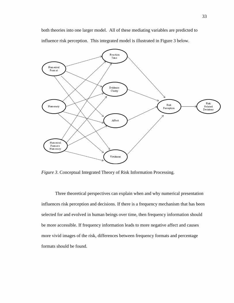
both theories into one larger model. All of these mediating variables are predicted to

influence risk perception. This integrated model is illustrated in Figure 3 below.

Figure 3. Conceptual Integrated Theory of Risk Information Processing.

Three theoretical perspectives can explain when and why numerical presentation

influences risk perception and decisions. If there is a frequency mechanism that has been

selected for and evolved in human beings over time, then frequency information should

be more accessible. If frequency information leads to more negative affect and causes

more vivid images of the risk, differences between frequency formats and percentage

formats should be found.

34

Hypotheses

Predictions of the Evolutionary Model

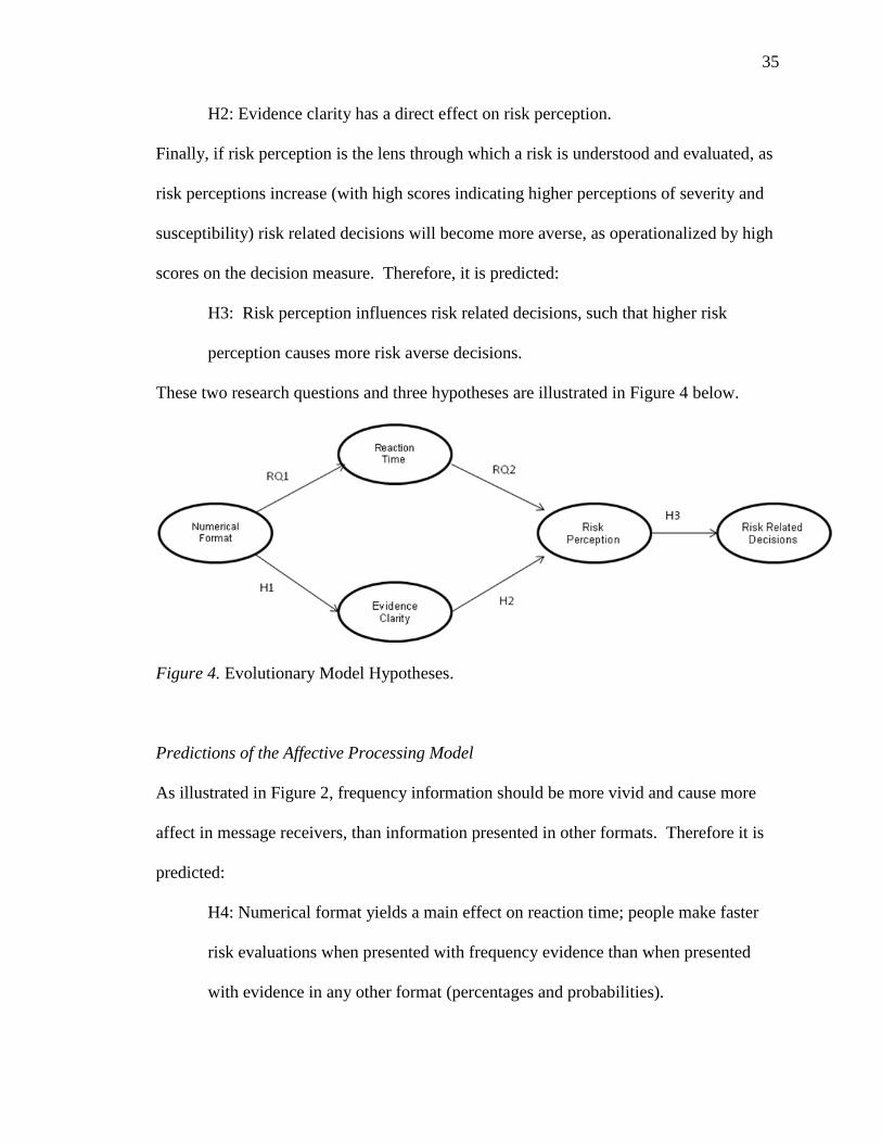
As illustrated in Figure 1, the evolutionary perspective implies that if people have

developed a cognitive mechanism for processing frequency information, frequency

formats should promote faster and easier evaluation of numerical evidence. Frequencies

facilitate reasoning because they reduce the number of required mathematical

computations. The information is natural in the sense that it corresponds to how humans

have experienced statistical information over the course of evolutionary history

(Gigerenzer & Hoffrage, 1995). The speed with which information is processed may have

implications for how a risk is perceived and evaluated. Therefore, research questions one

and two ask:

RQ1: Do people make faster risk evaluations when provided with frequency

evidence, than when provided with evidence in other formats (percentages and

probabilities)?

RQ2: Does the speed of reaction time influence risk perception?

Given the way that the human mind processes numbers, the evolutionary perspective

argues that the frequency format is more transparent than other formats (e.g., Brase,

2002; Cosmides & Tooby, 1996). The clarity of the numerical evidence is predicted to

influence perception about the risk and subsequently, risk related decisions. Specifically,

it is predicted that:

H1: When risk evidence is presented in a frequency format, the evidence will be

rated as clearer than when the evidence is presented in other formats (percentages

or probabilities).

35

H2: Evidence clarity has a direct effect on risk perception.

Finally, if risk perception is the lens through which a risk is understood and evaluated, as

risk perceptions increase (with high scores indicating higher perceptions of severity and

susceptibility) risk related decisions will become more averse, as operationalized by high

scores on the decision measure. Therefore, it is predicted:

H3: Risk perception influences risk related decisions, such that higher risk

perception causes more risk averse decisions.

These two research questions and three hypotheses are illustrated in Figure 4 below.

Figure 4. Evolutionary Model Hypotheses.

Predictions of the Affective Processing Model

As illustrated in Figure 2, frequency information should be more vivid and cause more

affect in message receivers, than information presented in other formats. Therefore it is

predicted:

H4: Numerical format yields a main effect on reaction time; people make faster

risk evaluations when presented with frequency evidence than when presented

with evidence in any other format (percentages and probabilities).

36

H5: Numerical format yields a main effect on affect, such that frequency evidence

leads to more negative affect compared to evidence presented in other formats

(percentages and probabilities).

H6: Numerical format will yield a main effect on vividness, such that frequency

evidence will be more rated as more vivid than evidence presented in other

formats (percentages and probabilities).

Differences based on objective numeracy have been found to influence information

processing. Compared to less numerate people, highly numerate people are more likely to

deliberate and think about numerical evidence. Less numerate people lack a clear

understanding of numbers and are more likely to make fast (System 2) evaluations and

form perceptions quickly (Peters et al., 2006). The affective processing paradigm

predicts that less numerate people will experience stronger negative affect when

presented with numerical information. More numerate people will have more neutral

feelings because they can draw more precise meaning from the numbers. People with low

numeracy are more influenced by irrelevant affective sources. In addition, compared to

less numerate people, highly numerate people are expected to extract more vividness

from numerical information (Peters, Lipkus, & Diefenbach, 2006; Slovic et al., 2000).

Peters et al. (2006) explained that when low numeracy people are presented with numbers

they lack the complexity and richness in understanding that is available to people with

high numeracy. Therefore, it is predicted that:

H7: Numeracy yields a main effect on reaction time; as numeracy increases,

reaction time increases linearly (highly numerate people spend more time

deliberating about a risk).

37

H8: Numeracy yields a main effect on affect, such that people with lower

numeracy have more negative affect from numerical risk information and people

with higher numeracy have more neutral affect from numerical risk information.

H9: Numeracy yields a main effect on vividness, such that people with high

numeracy have more vivid images of a risk when provided with any numerical

information than people with lower numeracy.

If numerical format influences reaction time, and lower numerate people respond

differentially to certain formats, then people with lower numeracy should react faster to

evidence in these formats. In contrast, people with higher numeracy should have no

reaction time differences based on format. These people have cognitive access to any

numerical format, not only the one they have been given. In addition, numerical format

and numeracy will interact to influence the feelings and vividness experienced. Highly

numerate people should have equal cognitive access to all numerical formats (Peters,

Västfjäll, et al., 2006). Thus, presentation format should not influence the amount of

vividness reported or affect experienced for people with higher numeracy. Thus, people

with lower numeracy, though, will only have cognitive access to the format they are

provided (i.e., they will not or cannot transform the numbers). People with lower

numeracy will derive more vividness and experience more affect from frequency

information, compared to other numerical formats.

38

H10: Numerical format and numeracy interact to influence reaction time, such

that lower numerate people make faster (System 2) risk evaluations when

provided with frequency evidence, compared to evidence presented in other

numerical formats (percentages and probabilities); whereas, people with higher

numeracy have no reaction time differences based on evidence format.

H11: Numerical format and numeracy interact to influence affect such that people

with lower numeracy have more negative affect from frequency evidence,

compared to evidence presented in other numerical formats (percentages and

probabilities); whereas, people with higher numeracy will have no affect

differences based on format.

H12: Numerical format and numeracy interact to influence vividness ratings, such

that people with lower numeracy will report more vividness when provided with

frequency evidence, compared to evidence presented in other numerical formats

(percentages and probabilities); whereas, people with higher numeracy will have

no vividness differences based on format.

According to the affective processing paradigm, when a person is presented with

information about a risk, informative signals about the qualities of a risk are felt.

Heuristic evaluations are intuitive, nonanalytical, and require minimal processing speed.

Faster processing of information has implications for risk perception; people should form

different evaluations if they spend time cognitively processing the evidence than if they

make immediate or automatic evaluations. Therefore it is predicted:

H13: Reaction time influences risk perception; a longer response time is

associated with lower risk perception.

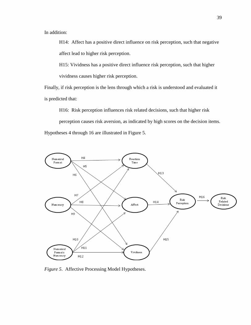
39

In addition:

H14: Affect has a positive direct influence on risk perception, such that negative

affect lead to higher risk perception.

H15: Vividness has a positive direct influence risk perception, such that higher

vividness causes higher risk perception.

Finally, if risk perception is the lens through which a risk is understood and evaluated it

is predicted that:

H16: Risk perception influences risk related decisions, such that higher risk

perception causes risk aversion, as indicated by high scores on the decision items.

Hypotheses 4 through 16 are illustrated in Figure 5.

Figure 5. Affective Processing Model Hypotheses.

40

Predictions of the Integrated Model

The integrated model predicts that reaction time, clarity, affect, and vividness all

influence risk perception or a person‘s beliefs about a risk. In addition to the preceding

predications, the integrated model includes two additional paths that hypothesize:

H17: Numeracy yields a main effect on evidence clarity, such that people with

higher numeracy evaluate numerical evidence as clearer than people with lower

numeracy.

H18: Numerical format and numeracy interact to influence evidence clarity, such

that lower numerate people evaluate evidence as clearer when it is presented in

frequency formats; whereas, people with higher numeracy have no clarity

differences based on format.

Figure 6. Integrated Model Hypotheses

41

Chapter IV: Pilot Study

This chapter describes the project‘s pilot study. The purpose of the pilot study

was to pre-test the messages that were proposed for use in the main experiments. This

study and the subsequent experiments were approved by the University of Maryland‘s

Institutional Review Board.

Pilot Study Method

A pilot study was designed to obtain information about the messages proposed for

use in the main experiments. This dissertation contains two main experiments that test

the predictions put forward by the evolutionary model, the affective processing model,

and the integrated model. The two experiments employ scenarios and measures

previously used by Brase (2002) and Slovic et al. (2000). The Brase and Slovic et al.

studies were chosen because the respective scholars (or team of scholars) are the

dominant adherents to the theories being empirically tested. Due to the fact that these

messages and measures have already been employed in experiments posited to be

consistent with the respective theories, it is logical to use these messages and measures to

explore the variables that mediate the relationship between numerical format and risk

perception, as well as numeracy and risk perception.

For Study 1, the topics of disease prevalence and drug efficacy from Brase (2002)

were pre-tested with a college age population. For Study 2, a modified version of the

Slovic et al. (2000) ―Mr. Jones‖ vignette was pre-tested. In the original ―Mr. Jones‖

study, participants were psychologists and psychiatrists who were presented with risk

evidence about Mr. Jones, a mental patient who committed a violent act. Risk evidence

was provided in one of two formats (a frequency or a percentage) and participants were

asked to make an assessment about the risk of Mr. Jones committing another violent act.

42

Due to the fact that the sample being studied in this dissertation project was significantly

different than Slovic et al. (2000) sample, the topic of the ―Mr. Jones‖ study was

modified to create a scenario that would have high involvement for to a college age

population. Thus, a vignette describing a University of Maryland student was developed.

In the vignette, a student committed a violent act and was expelled from the University.

Participants were presented with evidence about the student in one of four numerical

formats and asked to make decisions either allowing the student to return to the

University of Maryland or let the expulsion stand. The essence of the case remained the

same. In the pilot study, name of the student in the vignette was pre-tested. The original

Slovic et al. study used a male name (James Jones) in the vignette. This study aimed to be

gender neutral and three names (Taylor, Cameron, and Jordan) were pre-tested to find a

name that could refer to either a male or a female student.

In addition, the three topics and messages were evaluated by the pilot study

participants for realism. Open ended questions allowed for feedback on message clarity

and suggestions for improvement. The entire survey instrument for the pilot study is

provided in Appendix A.

Pilot Study Participants

Forty-seven undergraduate students at the University of Maryland participated in

the pilot study (62.00% of the participants were female and 38.00% were male). In the

sample, 57.40% of participants were Caucasian or White, 19.10% were Asian, 10.60%

were African-American or Black, 8.50% were Hispanic or Latino, and 4.30% selected

more than one race or ethnicity. Freshman made up 42.60% of the sample, 23.40% were

43

sophomores, 19.10% were juniors and 14.90% were seniors. The mean age was 19.63

(SD = 1.27, Mdn = 19.00).

Pilot Study Procedure

After completing an informed consent form, participants read and evaluated three

messages, two from each topic in Study 1 and one message from Study 2. After

evaluating each of the three messages all participants completed demographic questions.

Pilot Study Results

Participants were asked to rate the realism of the messages using a scale from 0

(not realistic at all) to 100 (completely realistic). The disease prevalence message had a

mean rating of 75.53 (SD = 22.99) and the drug efficacy message had a mean rating of

50.77 (SD = 37.76). The violent student vignette had a mean realism rating of 72.28 (SD

= 24.20). Responses from the open ended questions indicated that a context was needed

for the messages in the Study 1. Several participants questioned the source of the

information.

Pilot results for the Study 2 vignette showed that participants imagined Jones as a

male most often (98.80% for Taylor, 100% for Jordan, and 91.70% for Cameron). When

asked if each name is typically a man‘s name, woman‘s name, or could be used for both

sexes, 14.40% said that Taylor is typically a man‘s name, 25.50% said that Taylor was

typically a woman‘s name, and 59.60% replied that name could be used for both sexes.

For Jordan, 66.00% reported that the name is typically used for men and 34.00%

indicated that the name can be used for both sexes. No participants reported that the name

can be used for both men and women. For Cameron, 48.90% reported that the name is

44

typically used for men, 12.80% reported that the name is typically used for women, and

38.30% reported that the name is used for both men and women.

Modifications to the Messages

Based on these results, modifications were made to the messages. To the drug

efficacy and disease prevalence messages, the following sentence was added: ―The

following information is a recent New York Times newspaper headline‖. The goal of

this addition was to provide a context for the participants, albeit minimal. This provided

an explanation regarding why the message was brief. The name Taylor Jones was

selected for use in the Study 2 vignette.

45

Chapter V: Study 1

Method

Overview

Study 1 was based on Brase‘s (2002) work that compared and tested four

numerical formats: simple frequencies, natural frequencies, percentages, and

probabilities. Brase found that simple frequencies and percentages were rated clearer than

probabilities and natural frequencies. In the current research, a more comprehensive

measure of clarity was used (Brase used a one item measure) and reaction time, a variable

that emerged as important to the theories from the extant literature was included. In

Brase‘s original study, participants were provided with one of four pieces of numerical

evidence in the context of four unique situations (disease prevalence, drug efficacy,

marketing, and education). Two of the four topics, disease prevalence and drug efficacy,

that are relevant to risk communication, were used in this dissertation project.

Data collection for Study 1 was carried at the University of Maryland between

April 2010 and November 2010. The data from Study 1 was used to test all three of the

proposed models (the evolutionary model, the affective model, and the integrated model).

Design

A 2 (contexts: disease prevalence and drug efficacy) x 4 (numerical format:

simple frequency, natural frequency, probability, and percentage) independent groups

factorial design was implemented. Numeracy was a measured (versus indicated)

independent variable.

46

Participants

Participants were 553 students at the University of Maryland. Females made up

56.00% of the sample and the mean age was 19.78 (SD = 1.89, Mdn = 19.00, minimum =

18, maximum = 40). Most participants were White or Caucasian (60.60%), 13.20% were

Asian or Pacific Islander, 14.80% were Black or African American, 4.70% were Hispanic

or Latino, 0.09% were Middle Eastern, 0.02% were Native American, 4.50% indicted

more than race or ethnicity, and 0.09% of participants did not provide a response to this

open ended question. Of the 553 participants, 30.90% of the participants were freshman,

27.30% were sophomores, 23.50% were juniors, 17.60% were seniors, 0.07% were

graduate students, and 0.05% did not provide a response to this question. Participants

signed up to participate in the study using the Department of Communication‘s online

participant pool. In an effort to make the sample more diverse, students were asked to

bring a friend to the study who was not a communication major. Communication majors

made up 21.70% of the final sample. Students in the participant pool received course

credit in exchange for their participation in this study. Any student who could not receive

course credit had the option of entering a drawing for a $200 gift card.

Procedure

Participants signed up for a time slot online and reported to the Center for Risk

Communication Research lab in groups of 10. After signing in, all participants

completed an informed consent form. When all 10 participants arrived to the lab they

were seated at computer stations. Once participants started the study, they were

randomly assigned to an experimental condition by the DirectRT computer program.

47

Both the researcher and the participants were blind to the experimental condition. This

resulted in each participant receiving one piece of numerical evidence in one risk context.

After reading the experimental scenario, participants completed measures for each

of the dependent variables of interest (see Appendix B). Participants were instructed to

answer questions using either their computer keyboard or a button box that was attached

to their computer. The nine response buttons on the button box corresponded with

answer choices on the computer screen. For all items, reaction time was measured as the

time in milliseconds it took participants to answer each question. Demographic

information including age, year in school, and college major was also collected. The

complete protocol for Study 1 is provided in Appendix B.

Independent Variables

Experimental Scenarios

Participants were given one piece of risk evidence that was provided in one of

four numerical formats: a natural frequency, a simple frequency, a probability, and a

percentage. Each participant read one headline about one of the two topics (284

participants read the disease prevalence headline and 269 participants read the drug

efficacy headline). Participants were equally divided between experimental conditions:

129 participants received the simple frequency headlines, 140 participants received the

natural frequency headlines, 140 participants received the percentage headlines, and 144

participants received the probability headlines. All eight headlines are provided below.

Natural Frequency Headlines

Disease Prevalence: It is estimated that by the year 2020, 2.7 million of all U. S.

Americans will have been exposed to Flu strain X.

48

Drug Efficacy: A new drug is about to be approved by the FDA. It has been

estimated to cause negative side effects in 263 million of all U.S. Americans.

Simple Frequency Headlines

Disease Prevalence It is estimated that by the year 2020, 1 out of 100 U. S.



estimated to cause negative side effects in 99 of every 100 U.S. Americans.

Percentage Headlines

Disease Prevalence: It is estimated that by the year 2020, 1% of all U.S.



estimated to cause negative side effects in 99% of all U.S. Americans.

Probability Headlines

Disease Prevalence: It is estimated that by the year 2020, any given U.S.

American will have a probability of 0.01 of having been exposed to Flu strain X.


estimated to have a probability of 0.99 to cause negative side effects in any given

U.S. American.

Numeracy

Objective numeracy was measured using a 15-item expanded numeracy scale

developed by Schwartz et al. (1997), Lipkus, Samsa, and Reimer (2001), and Peters,

Dieckmann, Västfjäll, Mertz, and Slovic (2009). This measure is similar to a math test;

questions were scored as correct (1) or incorrect (0). This 15-item scale provides a

49

numeracy score with the potential to range from 0 - 15 for each participant. In this

sample, scores ranged from 2 to 15 (M = 11.06, SD = 2.14, Mdn = 12). A high score on

the scale is indicative of high objective numeracy and a low score represents low

objective numeracy. Objective numeracy was included as a continuous variable for most

analyses. When indicated, a median split was used to examine differences between

higher numeracy and lower numeracy (high numeracy = 12 – 15, low numeracy = 2 –

11).

Preference for Numerical Information: Subjective Numeracy

Preference for numerical information was measured using a 13-item subjective

numeracy measure developed by Fagerlin, Zikmund-Fisher, Ubel, Jankovic, Derry, and

Smith (2007). This is a subjective measured that evaluated participants‘ preference for

numerical information. A mean score was created for each participant (M = 6.00, SD =

1.44, Mdn = 6.23, minimum = 1.44, maximum = 9.00). A high score on the scale (9)

indicates a preference for numerical information and a low score (0) indicates a

preference for non numerical information. Cronbach‘s alpha reliability for these 13 items

was .86. Preference for information was correlated with objective numeracy (r = .48, p <

.01)

Numerical Format by Objective Numeracy Interaction Term

A numerical format by objective numeracy interaction term was created for use in

the causal models. Objective numeracy was included in the interaction term because this

variable was proposed to be part of the affective processing model (subjective numeracy

was not proposed as part of this theory). To create the interaction term, the continuous

variable (objective numeracy) was first mean centered. If the variable was not mean

50

centered, the interaction term would be highly correlated with the objective numeracy

variable and problems with multicollinearity could occur when both variables were

included in the causal models. To center the variable, the mean objective numeracy score

was subtracted from each participant‘s individual score. The interaction product term was

created by multiplying the centered variable and the categorical (numerical format)

variable (Cortina, Chen, & Dunlap, 2001).

Dependent Variables

Thought Listing

Using a procedure modified from Benthin, Slovic, Moran, Severson, Mertz, and

Gerrard (1995), participants were asked to list the first five images that came to mind

after reading the headline. For each image that was listed, participants were asked:

Using a scale from 0 - 100, how positive is this image (0 = completely negative, 100 =

completely positive), how clear is this image (0 = completely fuzzy, 100 = completely

clear), and how intense is this image (0 = weak, 100 = strong). The mean rating on the

negative/positive scale was 35.34 (SD = 20.47, minimum = 0, maximum = 100). The

mean rating on the fuzzy/clear scale was 69.25 (SD = 18.59, minimum = 0, maximum =

100) and the mean rating on the weak/strong intensity scale was 59.70 (SD = 17.68,

minimum = 1.00, maximum = 100). The average number of words used for each image

was 2.55 (SD = 1.93, Mdn = 1.80, minimum = 1.00, maximum = 15.80) and the mean

number of words used in the entire image listing task, for all five images, was 12.73 (SD

= 9.67, minimum = 5.00, maximum = 79.00).

51

Evidence Clarity

Perceived clarity of the evidence was measured with nine items. Brase‘s (2002)

one item clarity measure asked ―how clear and easy to understand is the statistical

information presented in the headline‖ (1 = unclear, 9 = clear). The mean score for this

item was 7.23 (SD = 1.93, Mdn = 8.00, minimum = 1, maximum = 9). In addition to this

one item, participants completed Hample‘s (2006) multi-item clarity scale. Participants

rated the evidence in the message with eight semantic differential items (unclear/clear,

confusing/not confusing, hard to understand/easy to understand, vague/precise, not a

noticeable point/a noticeable point, weak/strong, abstract/concrete, not relevant to the

conclusion/relevant to the conclusion). A high score indicates that the evidence in the

message was evaluated as clear to the reader; whereas, a low score is indicative of

unclear evidence. Cronbach‘s alpha reliability for the Hample scale was .86 (M = 4.54,

SD = 1.78, Mdn = 4.5, minimum = 1, maximum = 9).

Vividness

Vividness of the risk was measured with seven items on 0 - 100 scales (fuzzy,

detailed, vivid, intense, lifelike, sharp, and well-defined). A high score on the scale (100)

indicates high perceived vividness and a low score (0) indicates low perceived vividness.

Cronbach‘s alpha reliability for these seven items was .64 (M = 41.80, SD = 18.68, Mdn

= 41.43, minimum = 0, maximum = 100).

Affect

Affect was measured with nine semantic differential items adapted from Roskos-

Ewoldsen, Yu, and Rhodes (2004). In the disease prevalence condition, participants were

asked to respond to the statements: ―Flu strain X is‖ and ―Dedicating resources to dealing

52

with Flu strain X is.‖ Appendix B provides the questions for the drug efficacy conditions.

Response scales included: positive/negative, bad/good, beneficial/harmful, safe/unsafe,

wise/foolish, undesirable/desirable, tense/calm, annoyed/pleased, and

delighted/disgusted. A high score is indicative of positive affect and a low score is

indicative of negative affect about the risk. Cronbach‘s alpha reliability for these nine

items was .76 (M = 4.08, SD = 1.14, Mdn = 4.11, minimum = 1.00, maximum = 7.22).

Risk Perception

Risk perception is a multidimensional construct, typically conceptualized as

perceived susceptibility and perceived severity. Perceived susceptibility is an individual's

assessment of his or her risk and perceived severity is an individual's assessment of the

seriousness of the risk and its potential consequences (Rosenstock, 1966). Using the

items modified from Real (2008) and Rimal and Real (2003), risk perception was

measured with three perceived severity and three perceived susceptibility items. In the

disease prevalence conditions, items included: ―Using a scale from 0 (impossible to

happen) to 100 (certain to happen) how certain are you that you will be exposed to Flu

strain X?‖, ―Using a scale from 0 (impossible to happen) to 100 (certain to happen) what

is the chance that you will be exposed to Flu strain X?‖, and ―Using a scale from 0

(impossible to happen) to 100 (certain to happen) how likely is it that you will be exposed

to Flu strain X?‖. See Appendix B for the drug efficacy items. Perceived severity was

also measured with three items. In the disease prevalence conditions items included:

―Using a scale from 0 (impossible to happen) to 100 (certain to happen) what is the risk

of being exposed to Flu strain X?‖, ―Using a scale from 0 (impossible to happen) to 100

(certain to happen) how dangerous is Flu strain X?‖, and ―Using a scale from 0

53

(impossible to happen) to 100 (certain to happen) how serious is the existence of Flu

strain X?‖. A high score reflects high risk perception. Cronbach‘s alpha reliability for

these six items was .93 (M = 57.33, SD = 30.35, Mdn = 63.33, minimum = 0, maximum =

100).

Risk Related Decisions

Brase‘s (2002) outcome measure was used to assess risk related decision making.

Participants were asked to decide how much money should be allocated to each risk

situation. For the disease prevalence topic, participants were asked ―If you were in charge

of the annual budget for the U.S. Department of Health, how much of every $100 would

you dedicate to dealing with Flu strain X?‖. For the drug efficacy topic participants were

asked ―If you were in charge if the production budget for the manufacturer of this drug,

how much of every $100 would you dedicate to producing this drug?‖. The drug efficacy

item was re-coded so that more money allocated indicted risk aversion for both topics.

The values on this outcome variable ranged from 0 to 100 dollars (M = 43.75, SD =

36.03, Mdn = 40.00). In addition to this measure, participants completed two more

decision items on 1 (low risk) to 9 (high risk) scales (r = .14, p < .01, M = 5.76, SD =

1.64, Mdn = 5.50, minimum = 1.00, maximum = 9.00). These items are provided in

Appendix B.

Reaction Time

Participants completed all items on computers that were equipped with response

time software. Speed of response in milliseconds was measured for all questions in this

study. Mean speed in milliseconds for the six risk perception items described above was

54

used as the reaction time variable (M = 8225.59, SD = 3349.32, Mdn = 7682.60,

minimum = 1063.20, maximum = 30447.40).

Study 1 Data Analysis

This section is divided into two parts. The first part describes the preparation of

the data for Study 1. The second part presents the primary data analysis: the replication

of Brase (2002) and the tests of the hypotheses with the Study 1 data.

Preliminary Analyses

The frequencies of all observed variables were examined to look for errors. After

compiling the data set, 24 participants from Study 1 and 20 participants from Study 2 had

incomplete data files. The responses in these files did not record properly from the

DirectRT computer program. The missing data did not show a systematic pattern (e.g.,

no particular experimental condition and no particular questions) and these participants

were removed from the analysis. All other participants (553 from Study 1 and 395 from

Study 2) had complete data files for all items used in the analyses. The reaction time

items had to be transformed to reduce skewness. Reaction time scores are typically

clustered at one end of the scale. This was the case with this data as well. A logarithmic

transformation was used, reducing the skewness from 2.06 to - 0.08. When mean

reaction time scores are discussed, the un-transformed values are provided for clarity.

Data Analysis Plan

A two stage data analysis procedure was used to test the three causal models

described in this project (see Figures 1, 2, and 3). LISREL 8.80 (Joreskog & Sorbom,

2006) was used in both stages. The model parameters were estimated using maximum

likelihood procedures. In the first stage, the adequacy of the measurement models was

55

assessed using Confirmatory Factor Analysis (CFA). In all of the measurement models,

all latent variables were allowed to correlate freely and a metric assumption was made by

fixing one indicator item from each variable equal to 1. The statistical significance of the

parameter estimates was established by use of the t-statistic (the parameter divided by its

standard error). At the .05 level, the test statistic needs to be greater than |1.96| for the

parameter estimate to be statistically significant. In addition, squared multiple

correlations (R2) were examined for each of the observed measures. Squared multiple

correlations represent the extent to which a measured item explains a latent construct.

These values range from 0 to 1.

Four fit indices were used to evaluate the models: model chi square (χ2), an

incremental fit index (CFI), an absolute fit index (SRMR), and a parsimonious fit index

(RMSEA). The goodness of fit criteria used in this project are based on the

recommendations made by Hu and Bentler (1999). The χ2 goodness of fit statistic was

used as a measure of fit between the sample covariance and fitted covariance matrices. A

high probability associated with the χ2 test indicates a good model fit (Bollen, 1989).

Although the χ2 will be reported as an indicator of model fit, some researchers argue that

this is not appropriate measure of model fit for samples larger than 200 participants

(Kline, 2005). Given that both samples in this project are larger than 200, three additional

indices will be used to assess model fit. The CFI index was used to evaluate the absolute

fit of the model. This is the degree to which the unexplained variance remaining in the

model, after fitting, is substantial (Maruyama, 1998). The CFI index ranges from 0 to 1,

and values greater than or equal to .95 indicates a good model fit (Hu & Bentler, 1999).

The SRMR fit index is a measure of the standardized difference between the observed

56

covariance matrix and the predicted covariance matrix. A SRMR of 0 indicates a perfect

fit. A SRMR less than .08 is indicative of a good model fit (Hu & Bentler, 1999). Finally,

the RMSEA index evaluates the parsimony of the model. Hu and Bentler (1999)

recommend that a model has a good fit if the RMSEA value is less than or equal to .06.

After testing the proposed models, standardized residuals and modification

indices were examined for ways to improve the fit of the models. Residuals represent a

discrepancy between the observed and fitted covariance values and removing measures

with large standardized residuals will improve the fit of the model (Byrne, 1998). Large

residuals represent a misspecification in the model. In LISREL, a modification index is

provided for each parameter. This index provides a measure of how much a model‘s χ2 is

expected to decrease if the parameter is set free (Jöreskog & Sörbom, 1999). In addition,

factor loadings can also be evaluated. Removing measures with small factor loadings

will improve the fit of the model. The goal is to have a good fitting measurment model

before moving on to fitting the structural model to the data. However, it is important to

note that making modifications to a structural model moves the data analysis from a

confirmatory procedure to an exploratory procedure. The goal of this project was to test

the proposed theories. Therefore, modifications were made conservatively. Only

modifications that could be supported by the underlying theoretical frameworks were

made.

After establishing that the measured indicators explained the latent variables well,

the overall fit of the proposed structural models were tested. A Multiple Indicator

Multiple Cause (MIMIC) approach was used to examine the differences between the four

experimental conditions (four numerical formats). In a MIMIC model, dummy coded

57

variables are included in a model to differentiate between experimental groups. The

number of groups in the analysis is equal to the number of experimental groups minus

one. In this study, three coded variables were included in the model to represent three of

the experimental groups (simple frequencies, natural frequencies, and percentages).

These three groups were compared to the fourth group (probabilities). To conduct this

analysis, scores from all observed variables and all four experimental conditions were

combined together in one data set. A covariance matrix of the measured variables was

then computed. The covariance matrix contained the variances and covariances among

the measured indicators of the latent factors (reaction time, clarity, affect, vividness, risk

perception, and risk related decision), the covariances between the dummy coded

variables, and the variances of the dummy coded variables. This matrix contained both

the between-group covariance matrix among the means on the indicator variables in

addition to the within-group covariance matrix of indicator scores deviated about their

means. The covariance matrices for the final structural models are provided in

Appendices D through I.

To examine differences in factor means, the unstandardized parameter estimates

between the dummy coded variables and the latent factors these variables directly

influence were interpreted. If statistically significant paths were found, standardized

effect size statistics were evaluated to assess the strength of the effects (Hancock, 2001).

Two of the three models tested in this project included an interaction term.

Jöreskog and Yang (1996) recommend that one latent product indicator should be

included in a structural model as an interaction term. A format by objective numeracy

interaction product term was used in the affective processing model and the integrated

58

model. This interaction term has no real conceptual meaning; it is purely a tool for

examining a pattern of relationships among variables. The addition of an interaction term

in causal modeling leads to interrelatedness among predictor variables. This can cause a

multitude of problems related to identification and multicollineary. Cortina, Chen, and

Dunlap (2001) recommended mean centering all observed variables to avoid specification

problems. This strategy was used in this project to minimize the problems associated with

the addition of an interaction term in a causal model. In all of the structural models, the

observed variables were mean centered before data analysis.

The next section describes the analysis of the three causal models using the data

from Study 1. The variables and indicators are discussed by using shorted codes (e.g.,

DEC, CLARITY, SEV1). The actual items from the study are provided in the

Appendices B and C with the corresponding codes that are used throughout the following

sections.

Study 1 Results

Replication of Brase

Brase (2002) presented information to participants in one of four numerical

formats: simple frequencies (e.g. 1 in 3), probabilities (e.g. 0.33), percentages (e.g. 33%),

and natural frequencies for the US population (e.g. 90 million). Four risk topics were

used: disease prevalence, education, marketing, and drug efficacy. After reading the

information, participants responded to items that measured clarity (―how clear and easy

to understand was the statistical information‖) and monetary pull of the information.

Clarity was measured on a 5-point scale and monetary pull was measured by asking

participants to allocate an amount of money, out of 100 dollars, to the particular issue

59

discussed in the message. Brase found statistically significant differences in clarity

between the numerical formats. Post hoc analyses indicated that both simple frequencies

and percents were rated clearer than probabilities and natural frequencies.

In this project, participants were also presented with numerical evidence in one of

four numerical formats. After reading the information, participants were asked to respond

to Brase‘s clarity item (―How clear and easy to understand is the statistical information

presented in the headline?‖) and one monetary pull item. The clarity item was measured

on a 9-point scale and monetary pull was measured by asking participants to allocate an

amount of money out 100 dollars to the particular issue discussed in the message.

Statistically significant differences in clarity were also found between the numerical

formats, F (3, 552) = 14.41, p < .01, η2

= 0.07. The mean ratings for each condition are

provided in Table 1. Post hoc least squares difference (LDS) tests show that simple

frequencies, percents, and natural frequencies (M = 7.35, p < .01) were rated statistically

significantly clearer than probabilities, replicating the Brase (2002) findings.

Table 1

Means and Standard Deviations for Evidence Clarity by Numerical Format.

_______________________________________________________________________

Numerical Format Mean (SD)

________________________________________________________________________

Probabilities 6.31 (2.21)a

Simple Frequency 7.49 (1.84)b

Percent 7.69 (1.68)b

Natural Frequencies 7.35 (1.73)b

________________________________________________________________________

Note: a is significantly different than b, p < .01

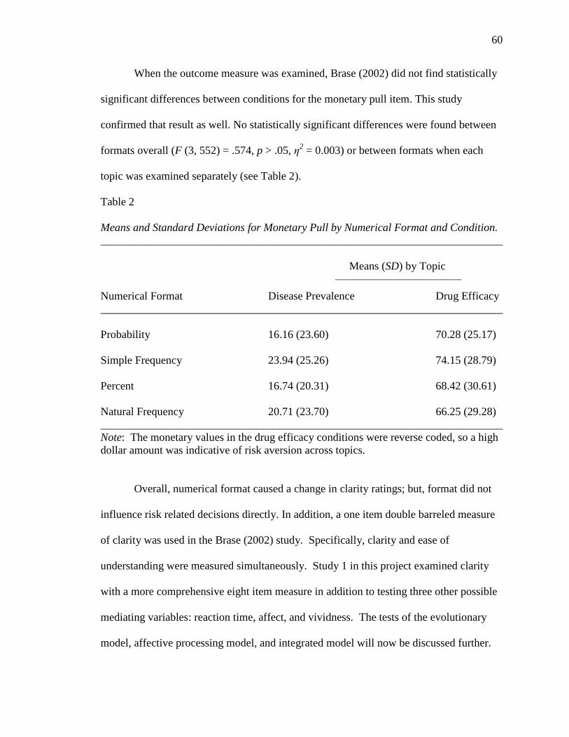
60

When the outcome measure was examined, Brase (2002) did not find statistically

significant differences between conditions for the monetary pull item. This study

confirmed that result as well. No statistically significant differences were found between

formats overall (F (3, 552) = .574, p > .05, η2 = 0.003) or between formats when each

topic was examined separately (see Table 2).

Table 2

Means and Standard Deviations for Monetary Pull by Numerical Format and Condition.

________________________________________________________________________

Means (SD) by Topic __________________________________

Numerical Format Disease Prevalence Drug Efficacy

________________________________________________________________________

Probability 16.16 (23.60) 70.28 (25.17)

Simple Frequency 23.94 (25.26) 74.15 (28.79)

Percent 16.74 (20.31) 68.42 (30.61)

Natural Frequency 20.71 (23.70) 66.25 (29.28)

________________________________________________________________________

Note: The monetary values in the drug efficacy conditions were reverse coded, so a high

dollar amount was indicative of risk aversion across topics.

Overall, numerical format caused a change in clarity ratings; but, format did not

influence risk related decisions directly. In addition, a one item double barreled measure

of clarity was used in the Brase (2002) study. Specifically, clarity and ease of

understanding were measured simultaneously. Study 1 in this project examined clarity

with a more comprehensive eight item measure in addition to testing three other possible

mediating variables: reaction time, affect, and vividness. The tests of the evolutionary

model, affective processing model, and integrated model will now be discussed further.

61

Evolutionary Measurement Model

The evolutionary measurement model included three latent variables (clarity, risk

perception, and risk related decisions). The proposed CFA model would not converge

with the data. To examine problems in the model, separate CFAs were conducted for

each latent variable and the corresponding indicators. The CFAs indicated that two of the

decision items (DEC2 and DEC3) were very highly correlated with the Brase (DEC1)

item. These two items were removed from the model and the Brase monetary pull item

that asked participants to indicate how many dollars out of 100 they would allocate to the

new flu or testing the new drug was retained and this item served as a single indictor of a

risk related decision.

The first estimation of the two factor (clarity and risk perception) measurement

model showed a poor fit to the data, χ2 (75, N = 553) = 1259.16, p < .01; CFI = .87;

SRMR = .12; RMSEA = .17. To examine problems in the model and look for ways to

improve model fit, the standardized residuals and modification indices were examined.

The items CLARITY3, CLARITY5, CLARITY6, CLARITY7, CLARITY8, and SEV3

(see Appendix B for these items) had large standardized residuals and were removed

from the model. The largest modification index was between the items SEV1 and SEV2

and the error between these variables was allowed to covary. These items share a similar

question stem and allowing the measurement errors between these items improved the fit

of the model. A second CFA was conducted with the three indicator clarity factor and

the five indictor risk perception factor. This resulted in a final measurement model that

had a good fit to the data based on the CFI, SRMR, and RMSEA fit indices, χ2 (18, N =

553) = 43.33, p < .01; CFI = .99; SRMR = .02; RMSEA = .05. In the final model, clarity

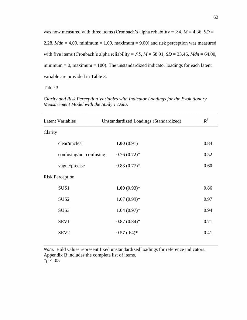
62

was now measured with three items (Cronbach‘s alpha reliability = .84, M = 4.36, SD =

2.28, Mdn = 4.00, minimum = 1.00, maximum = 9.00) and risk perception was measured

with five items (Cronbach‘s alpha reliability = .95, M = 58.91, SD = 33.46, Mdn = 64.00,

minimum = 0, maximum = 100). The unstandardized indicator loadings for each latent

variable are provided in Table 3.

Table 3

Clarity and Risk Perception Variables with Indicator Loadings for the Evolutionary

Measurement Model with the Study 1 Data.

________________________________________________________________________

Latent Variables Unstandardized Loadings (Standardized) R2

____________________________________________________________________________________________________________

Clarity

clear/unclear 1.00 (0.91) 0.84

confusing/not confusing 0.76 (0.72)* 0.52

vague/precise 0.83 (0.77)* 0.60

Risk Perception

SUS1 1.00 (0.93)* 0.86

SUS2 1.07 (0.99)* 0.97

SUS3 1.04 (0.97)* 0.94

SEV1 0.87 (0.84)* 0.71

SEV2 0.57 (.64)* 0.41

________________________________________________________________________

Note. Bold values represent fixed unstandardized loadings for reference indicators.

Appendix B includes the complete list of items.

*p < .05

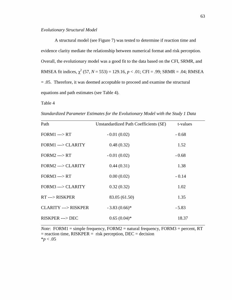
63

Evolutionary Structural Model

A structural model (see Figure 7) was tested to determine if reaction time and

evidence clarity mediate the relationship between numerical format and risk perception.

Overall, the evolutionary model was a good fit to the data based on the CFI, SRMR, and

RMSEA fit indices, χ2 (57, N = 553) = 129.16, p < .01; CFI = .99; SRMR = .04; RMSEA

= .05. Therefore, it was deemed acceptable to proceed and examine the structural

equations and path estimates (see Table 4).

Table 4

Standardized Parameter Estimates for the Evolutionary Model with the Study 1 Data

________________________________________________________________________

Path Unstandardized Path Coefficients (SE) t-values

FORM1 ---> RT - 0.01 (0.02) - 0.68

FORM1 ---> CLARITY 0.48 (0.32) 1.52

FORM2 ---> RT - 0.01 (0.02) - 0.68

FORM2 ---> CLARITY 0.44 (0.31) 1.38

FORM3 ---> RT 0.00 (0.02) - 0.14

FORM3 ---> CLARITY 0.32 (0.32) 1.02

RT ---> RISKPER 83.05 (61.50) 1.35

CLARITY ---> RISKPER - 3.83 (0.66)* - 5.83

RISKPER ---> DEC 0.65 (0.04)* 18.37

________________________________________________________________________

Note: FORM1 = simple frequency, FORM2 = natural frequency, FORM3 = percent, RT

= reaction time, RISKPER = risk perception, DEC = decision

*p < .05

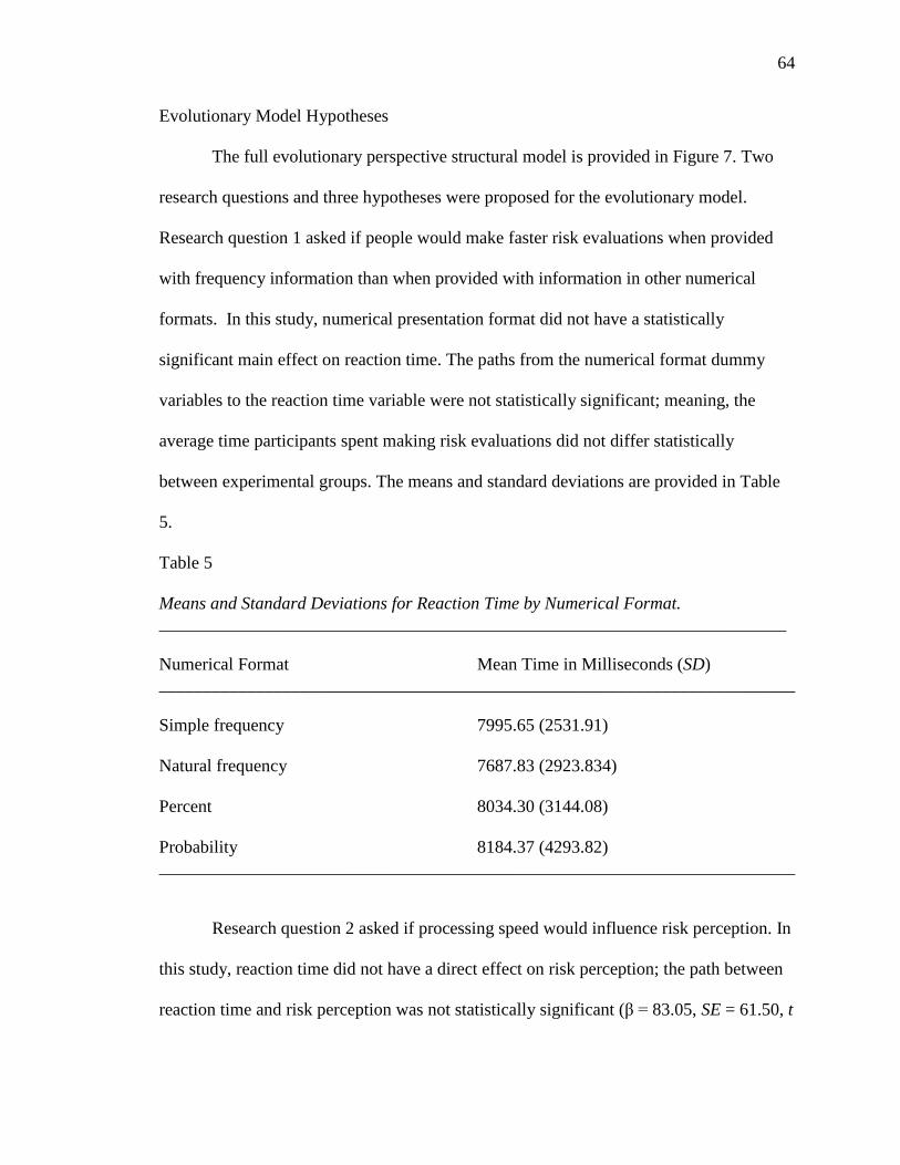
64

Evolutionary Model Hypotheses

The full evolutionary perspective structural model is provided in Figure 7. Two

research questions and three hypotheses were proposed for the evolutionary model.

Research question 1 asked if people would make faster risk evaluations when provided

with frequency information than when provided with information in other numerical

formats. In this study, numerical presentation format did not have a statistically

significant main effect on reaction time. The paths from the numerical format dummy

variables to the reaction time variable were not statistically significant; meaning, the

average time participants spent making risk evaluations did not differ statistically

between experimental groups. The means and standard deviations are provided in Table

5.

Table 5

Means and Standard Deviations for Reaction Time by Numerical Format.

_______________________________________________________________________

Numerical Format Mean Time in Milliseconds (SD)

________________________________________________________________________

Simple frequency 7995.65 (2531.91)

Natural frequency 7687.83 (2923.834)

Percent 8034.30 (3144.08)

Probability 8184.37 (4293.82)

________________________________________________________________________

Research question 2 asked if processing speed would influence risk perception. In

this study, reaction time did not have a direct effect on risk perception; the path between

reaction time and risk perception was not statistically significant (β = 83.05, SE = 61.50, t

65

= 1.35). The three evolutionary model hypotheses were then tested. Hypothesis 1

predicted that when risk evidence was presented in a frequency format the evidence

would be rated clear than when the evidence was presented as percentages or

probabilities. This hypothesis was not supported by these data. Numerical format did not

a have a statistically significant main effect on evidence clarity, as shown by the three

nonsignificant coefficients in Table 4. ANOVA results confirm this finding, F (3, 552) =

1.08, p > .05, η2 = 0.006. For clarity, no statistically significant differences were found

between the four numerical formats.

Hypothesis 2 predicted that clarity has a direct effect on risk perception. The data

support this prediction. Evidence clarity was a statistically significant predictor of risk

perception (β = -3.83, SE = 0.66, t = -5.83). The negative sign of the path coefficient

indicates that, as ratings of evidence clarity increased, participants reported lower risk

perceptions. Finally, Hypothesis 3 predicted that as risk perceptions increase, decisions

will become more risk averse. This hypothesis was also supported. Risk perception

influenced the number of dollars participants chose to allocate to reducing a risk (β =

0.65, SE = 0.04, t = 18.37). The higher risk perception that participants felt, the more

money they were willing to dedicate to reducing the risk in the headline.

66

Figure 7. Evolutionary Structural Model with Standardized Path Coefficients with the

Study 1 Data. In the model the simple frequency, natural frequency, and percentage

variables represent three dummy variables that can be compared to the fourth message

condition, probability.

* p < .05

Affective Processing Measurement Model

The affective processing measurement model included three latent variables

(affect, vividness, and risk perception). Two pairs of vividness indicators had perfect

1.00 correlations (defined/intense and sharp/vivid). As a result, the indicators intense and

vivid were removed from the model before estimation. The first estimation of the

measurement model showed a poor fit to the data, χ2 (167, N = 553) = 2642.74, p < .01;

CFI = .77; SRMR = .16; RMSEA = .16. Standardized residuals were examined and

AFFECT2, AFFECT3, AFFECT5, AFFECT7, AFFECT8, AFFECT9, VIVIDNESS7,

VIVIDNESS8, and SEV3 were removed from the model (these items are provided in

Appendix B). As in the evolutionary model, the measurement error between SEV1 and

SEV2 was allowed to covary. These items share a similar question stem and allowing the

67

measurement errors between these items to covary improved the overall fit of the model.

This resulted in a final measurement model with three latent variables and 10 indicators.

This model had an acceptable fit based on the CFI, SRMR, and RMSEA fit indices and

was retained, χ2 (31, N = 553) = 97.27, p < .01; CFI = .98; SRMR = .05; RMSEA = .06.

In the final model vividness was measured with three indicators (Cronbach‘s alpha

reliability = .60, M = 37.54, SD = 25.21, Mdn = 36.67, minimum = 0, maximum = 100)

and affect was measured with two indictors (r = .47, p < .01, M = 2.66, SD = 1.52, Mdn =

2.50, minimum = 1.00, maximum = 8.50).

Table 6

Affect, Vividness, and Risk Perception Variables with Indicator Loadings for the Affective

Processing Measurement Model with the Study 1 Data

________________________________________________________________________


____________________________________________________________________________________________________________

Affect

negative/positive 0.64 (0.58) 0.34

undesirable/desirable 1.00 (0.81)* 0.65

Vividness

detailed 1.00 (0.89)* 0.79

vivid 0.77 (0.55)* 0.30

fuzzy 0.49 (0.36)* 0.13

Risk Perception

SUS1 0.93 (0.93)* 0.86

SUS2 1.00 (0.99) 0.97

SUS3 0.97 (0.97)* 0.94

SEV1 0.81 (0.84)* 0.70

68

SEV2 0.53 (.64)* 0.41

________________________________________________________________________



*p < .05

Affective Processing Structural Model

The affective processing structural model predicted that reaction time, affect, and

vividness mediate the relationship between the exogenous variables numerical format and

numeracy and the endogenous variables risk perception and risk related decision. Overall,

the data fit this model reasonably well based on the CFI, SRMR, and RMSEA indices, χ2

(105, N = 553) = 276.35, p < .01; CFI = .97; SRMR = .05; RMSEA = .05. Table 7

provides the structural equations and path estimates for the model.

Table 7

Standardized Parameter Estimates for the Affective Processing Model with the Study 1

Data

________________________________________________________________________


________________________________________________________________________

FORM1 ---> RT 0.03 (0.02) 1.55

FORM1 ---> AFFECT 0.07 (0.09) 0.76

FORM1 ---> VIVIDNESS - 0.33 (1.66) - 0.20

FORM2 ---> RT 0.03 (0.02) 1.55

FORM2 ---> AFFECT - 0.09 (0.09) - 0.92

FORM2 ---> VIVIDNESS 0.15 (1.65) 0.09

FORM3 ---> RT - 0.01 (0.02) - 0.48

FORM3 ---> AFFECT 0.14 (0.10) 1.40

FORM3 ---> VIVIDNESS 1.70 (1.69) 1.01

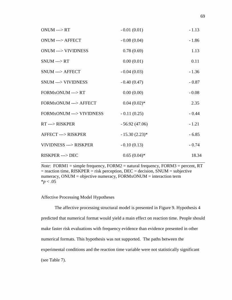
69

ONUM ---> RT - 0.01 (0.01) - 1.13

ONUM ---> AFFECT - 0.08 (0.04) - 1.86

ONUM ---> VIVIDNESS 0.78 (0.69) 1.13

SNUM ---> RT 0.00 (0.01) 0.11

SNUM ---> AFFECT - 0.04 (0.03) - 1.36

SNUM ---> VIVIDNESS - 0.40 (0.47) - 0.87

FORMxONUM ---> RT 0.00 (0.00) - 0.08

FORMxONUM ---> AFFECT 0.04 (0.02)* 2.35

FORMxONUM ---> VIVIDNESS - 0.11 (0.25) - 0.44

RT ---> RISKPER - 56.92 (47.06) - 1.21

AFFECT ---> RISKPER - 15.30 (2.23)* - 6.85

VIVIDNESS ---> RISKPER - 0.10 (0.13) - 0.74

RISKPER ---> DEC 0.65 (0.04)* 18.34

________________________________________________________________________


= reaction time, RISKPER = risk perception, DEC = decision, SNUM = subjective

numeracy, ONUM = objective numeracy, FORMxONUM = interaction term

*p < .05

Affective Processing Model Hypotheses

The affective processing structural model is presented in Figure 9. Hypothesis 4

predicted that numerical format would yield a main effect on reaction time. People should

make faster risk evaluations with frequency evidence than evidence presented in other

numerical formats. This hypothesis was not supported. The paths between the

experimental conditions and the reaction time variable were not statistically significant

(see Table 7).

70

Hypotheses 5 and 6 predicted that numerical format would yield main effects on

both affect and vividness. Overall, numerical format did not influence vividness or affect

in this study. As shown in Table 7, the paths between the numerical format dummy

variables and vividness and the numerical format dummy variables and affect were not

statistically significant. ANOVA results confirm these findings. Overall, there were no

statistically significant differences between numerical formats for affect (F (3, 552) =

1.54, p > .05, η2 = 0.008) or vividness (F (3, 552) = 0.95, p > .05, η

2 = 0.005). The data

from the image listing task support the conclusion that numerical format did not influence

the reported vividness of the risks. In this study, no statistically significant differences

were found between the experimental conditions and positivity of the reported images (F

(3, 536) = .50, p > .05, η2 = 0.003), clarity of the reported images (F (3, 540) = .96, p >

.05, η2 = 0.003), or intensity of the reported images (F (3, 532) = .12, p > .05, η

2 = 0.003).

Hypothesis 7 predicted that numeracy would yield a main effect on reaction time.

This hypothesis was not supported. Neither objective numeracy (β = - 0.01, SE = 0.01, t =

- 1.13) nor preference for numerical information (β = 0.00, SE = 0.01, t = 0.11) had

significant direct effects on the reaction time variable. When high and low objective

numeracy were compared using the numeracy median split variable, the two groups did

not differ statistically (t = -1.23, SE = .01, df = 551, p > .05).

Hypothesis 8 predicted that numeracy would yield a main effect on affect, such

that people with lower numeracy would experience more negative affect from numerical

risk information. This hypothesis was not supported by the causal model. Neither

objective numeracy (β = - 0.08, SE = 0.04, t = -1.86), nor preference for numerical

information (β = - 0.04, SE = 0.03, t = -1.36) had a direct influence on affect in the

71

model. However, when a median split was used to compare higher objective numeracy to

lower objective numeracy, statistically significant differences were found for reported

affects (t = 2.11, SE = .09, df = 551, p < .05). People with higher numeracy (M = 4.18,

SD = 1.10) experienced more positive/neutral affect; whereas, people with lower

objective numeracy reported more negative affect (M = 3.97, SD = 1.18). On the affect

scale, 1.00 is negative affect and 9.00 is positive affect.

Hypothesis 9 predicted that numeracy would have a main effect on vividness,

such that people with higher numeracy would report more vividness from numerical

information than people with lower numeracy. This hypothesis was not supported; neither

objective numeracy (β = 0.78, SE = 0.69, t = 1.13), nor preference for numerical

information (β = - 0.40, SE = 0.47, t = - 0.87) directly influenced vividness. When higher

and lower objective numeracy were compared using a median split, no statistically

significant differences were found for vividness (t = 0.78, SE = 2.14, df = 551, p > .05).

Hypothesis 10 predicted that numerical format and numeracy would interact to influence

reaction time. This prediction was not supported by the data (β = 0.00, SE = 0.00, t =

-0.08). ANOVA results using the median split variable corroborate this result, F (3, 553)

= 1.10, p > .05.

Hypothesis 11 predicted that numerical format and numeracy would interact to

influence affect. Specifically, it was predicted that people with lower numeracy would

report more negative affect from frequency information, compared to information

presented in other numerical formats. The numerical format by numeracy interaction term

did have a direct effect on reported affect (β = 0.04, SE = 0.02, t = 2.35). To determine

the nature of the interaction, a follow up test using ANOVA was conducted employing

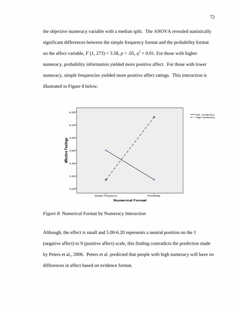
72

the objective numeracy variable with a median split. The ANOVA revealed statistically

significant differences between the simple frequency format and the probability format

on the affect variable, F (1, 273) = 3.58, p < .05, η2 = 0.01. For those with higher

numeracy, probability information yielded more positive affect. For those with lower

numeracy, simple frequencies yielded more positive affect ratings. This interaction is

illustrated in Figure 8 below.

Figure 8. Numerical Format by Numeracy Interaction

Although, the effect is small and 5.00-6.20 represents a neutral position on the 1

(negative affect) to 9 (positive affect) scale, this finding contradicts the prediction made

by Peters et al., 2006. Peters et al. predicted that people with high numeracy will have no

differences in affect based on evidence format.

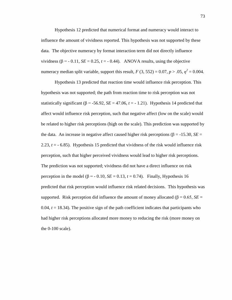
73


influence the amount of vividness reported. This hypothesis was not supported by these

data. The objective numeracy by format interaction term did not directly influence

vividness (β = - 0.11, SE = 0.25, t = - 0.44). ANOVA results, using the objective

numeracy median split variable, support this result, F (3, 552) = 0.07, p > .05, η2 = 0.004.

Hypothesis 13 predicted that reaction time would influence risk perception. This

hypothesis was not supported; the path from reaction time to risk perception was not

statistically significant (β = -56.92, SE = 47.06, t = - 1.21). Hypothesis 14 predicted that

affect would influence risk perception, such that negative affect (low on the scale) would

be related to higher risk perceptions (high on the scale). This prediction was supported by

the data. An increase in negative affect caused higher risk perceptions (β = -15.30, SE =

2.23, t = - 6.85). Hypothesis 15 predicted that vividness of the risk would influence risk

perception, such that higher perceived vividness would lead to higher risk perceptions.

The prediction was not supported; vividness did not have a direct influence on risk

perception in the model (β = - 0.10, SE = 0.13, t = 0.74). Finally, Hypothesis 16

predicted that risk perception would influence risk related decisions. This hypothesis was

supported. Risk perception did influence the amount of money allocated (β = 0.65, SE =

0.04, t = 18.34). The positive sign of the path coefficient indicates that participants who

had higher risk perceptions allocated more money to reducing the risk (more money on

the 0-100 scale).

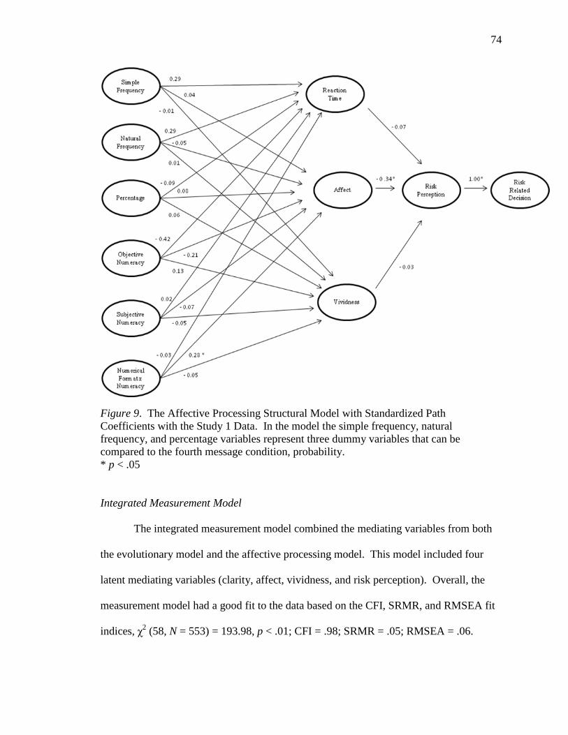
74

Figure 9. The Affective Processing Structural Model with Standardized Path

Coefficients with the Study 1 Data. In the model the simple frequency, natural

frequency, and percentage variables represent three dummy variables that can be

compared to the fourth message condition, probability.

* p < .05

Integrated Measurement Model

The integrated measurement model combined the mediating variables from both

the evolutionary model and the affective processing model. This model included four

latent mediating variables (clarity, affect, vividness, and risk perception). Overall, the

measurement model had a good fit to the data based on the CFI, SRMR, and RMSEA fit

indices, χ2 (58, N = 553) = 193.98, p < .01; CFI = .98; SRMR = .05; RMSEA = .06.

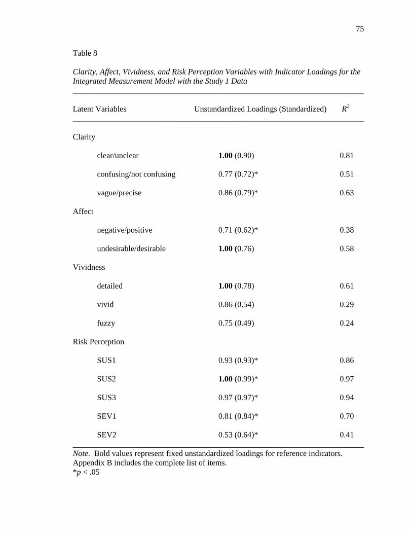
75

Table 8

Clarity, Affect, Vividness, and Risk Perception Variables with Indicator Loadings for the

Integrated Measurement Model with the Study 1 Data

________________________________________________________________________


________________________________________________________________________

Clarity



vague/precise 0.86 (0.79)* 0.63

Affect

negative/positive 0.71 (0.62)* 0.38

undesirable/desirable 1.00 (0.76) 0.58

Vividness

detailed 1.00 (0.78) 0.61

vivid 0.86 (0.54) 0.29

fuzzy 0.75 (0.49) 0.24

Risk Perception

SUS1 0.93 (0.93)* 0.86

SUS2 1.00 (0.99)* 0.97

SUS3 0.97 (0.97)* 0.94

SEV1 0.81 (0.84)* 0.70

SEV2 0.53 (0.64)* 0.41

________________________________________________________________________



*p < .05

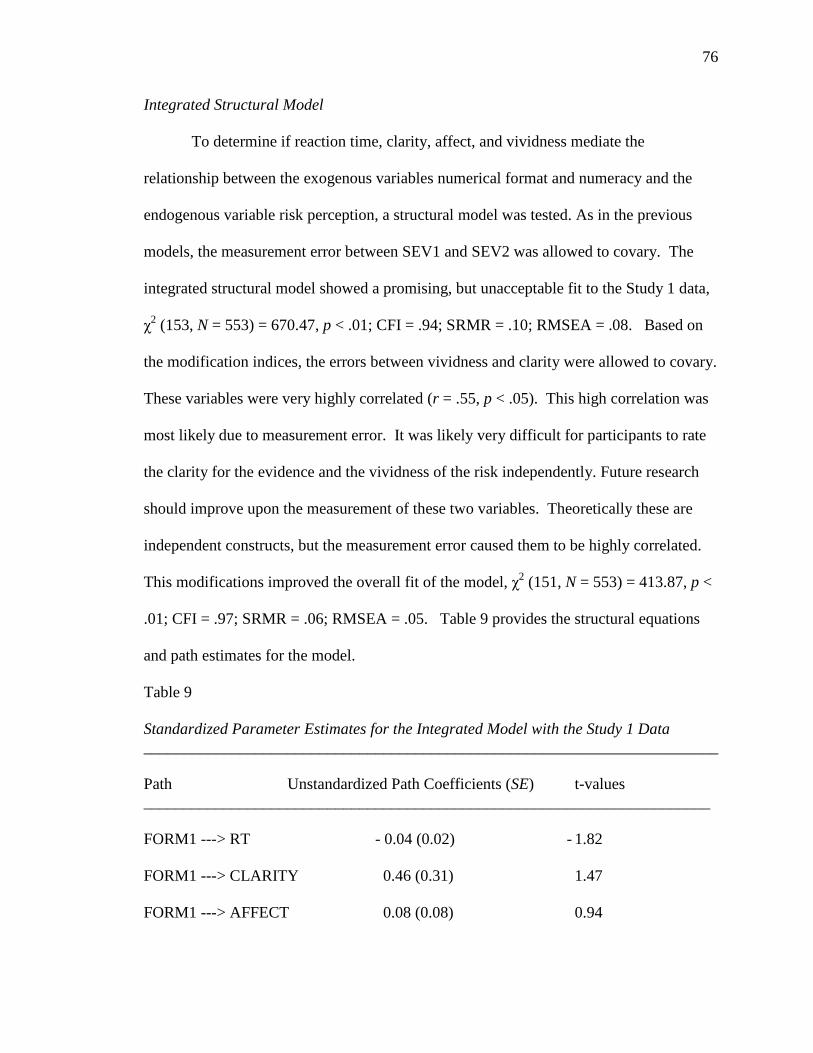
76

Integrated Structural Model

To determine if reaction time, clarity, affect, and vividness mediate the

relationship between the exogenous variables numerical format and numeracy and the

endogenous variable risk perception, a structural model was tested. As in the previous

models, the measurement error between SEV1 and SEV2 was allowed to covary. The

integrated structural model showed a promising, but unacceptable fit to the Study 1 data,

χ2 (153, N = 553) = 670.47, p < .01; CFI = .94; SRMR = .10; RMSEA = .08. Based on

the modification indices, the errors between vividness and clarity were allowed to covary.

These variables were very highly correlated (r = .55, p < .05). This high correlation was

most likely due to measurement error. It was likely very difficult for participants to rate

the clarity for the evidence and the vividness of the risk independently. Future research

should improve upon the measurement of these two variables. Theoretically these are

independent constructs, but the measurement error caused them to be highly correlated.

This modifications improved the overall fit of the model, χ2 (151, N = 553) = 413.87, p <

.01; CFI = .97; SRMR = .06; RMSEA = .05. Table 9 provides the structural equations

and path estimates for the model.

Table 9

Standardized Parameter Estimates for the Integrated Model with the Study 1 Data

________________________________________________________________________


_______________________________________________________________________

FORM1 ---> RT - 0.04 (0.02) - 1.82

FORM1 ---> CLARITY 0.46 (0.31) 1.47

FORM1 ---> AFFECT 0.08 (0.08) 0.94

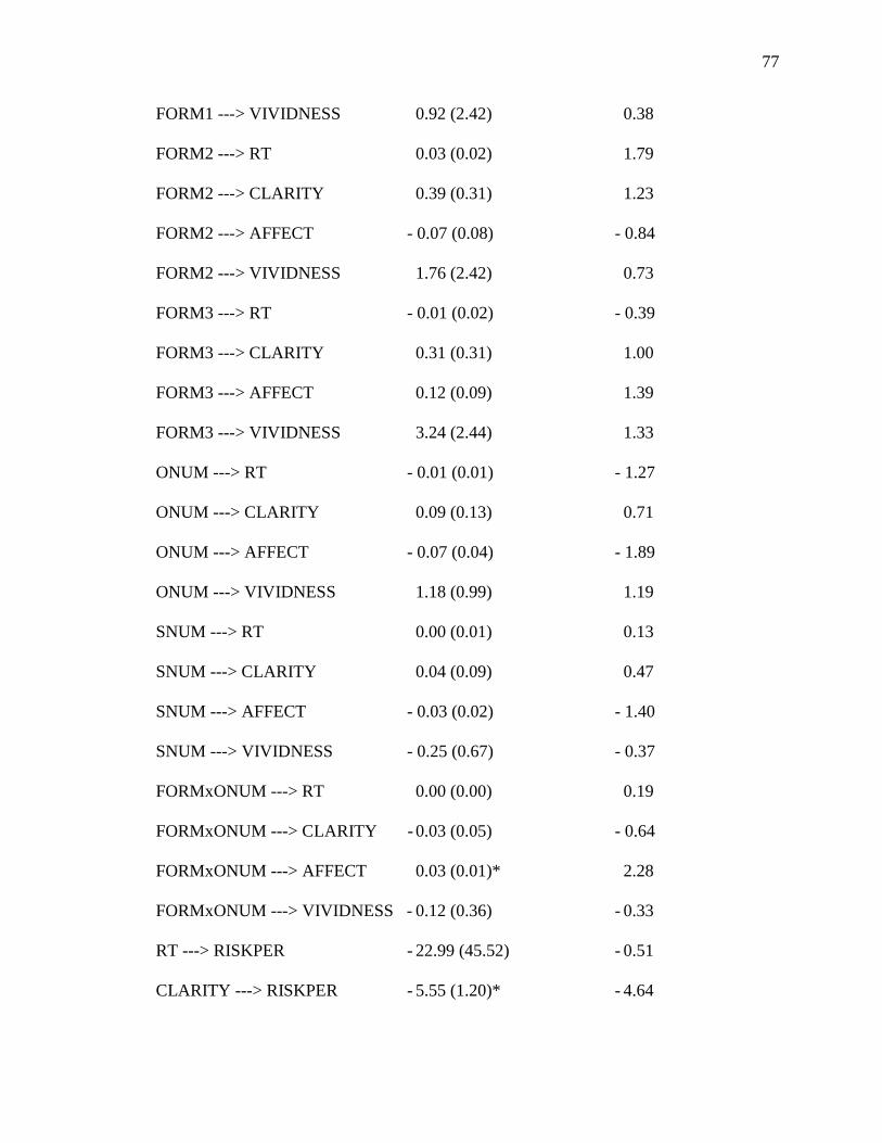
77

FORM1 ---> VIVIDNESS 0.92 (2.42) 0.38

FORM2 ---> RT 0.03 (0.02) 1.79

FORM2 ---> CLARITY 0.39 (0.31) 1.23

FORM2 ---> AFFECT - 0.07 (0.08) - 0.84

FORM2 ---> VIVIDNESS 1.76 (2.42) 0.73

FORM3 ---> RT - 0.01 (0.02) - 0.39

FORM3 ---> CLARITY 0.31 (0.31) 1.00

FORM3 ---> AFFECT 0.12 (0.09) 1.39

FORM3 ---> VIVIDNESS 3.24 (2.44) 1.33

ONUM ---> RT - 0.01 (0.01) - 1.27

ONUM ---> CLARITY 0.09 (0.13) 0.71

ONUM ---> AFFECT - 0.07 (0.04) - 1.89

ONUM ---> VIVIDNESS 1.18 (0.99) 1.19

SNUM ---> RT 0.00 (0.01) 0.13

SNUM ---> CLARITY 0.04 (0.09) 0.47

SNUM ---> AFFECT - 0.03 (0.02) - 1.40

SNUM ---> VIVIDNESS - 0.25 (0.67) - 0.37

FORMxONUM ---> RT 0.00 (0.00) 0.19

FORMxONUM ---> CLARITY - 0.03 (0.05) - 0.64

FORMxONUM ---> AFFECT 0.03 (0.01)* 2.28


RT ---> RISKPER - 22.99 (45.52) - 0.51

CLARITY ---> RISKPER - 5.55 (1.20)* - 4.64

78

AFFECT ---> RISKPER - 13.98 (2.16)* - 6.48

VIVIDNESS ---> RISKPER 0.51 (0.19)* 2.76

RISKPER ---> DEC 0.65 (0.04)* 18.20

_______________________________________________________________________


= reaction time, RISKPER = risk perception, DEC = decision, SNUM = subjective

numeracy, ONUM = objective numeracy, FORMxONUM = interaction term

*p < .05

In addition to the predictions put forth in the previous two models, the integrated

model included two additional paths represented by hypotheses 17 and 18 (the full

integrated structural model with standardized path coefficients is provided in Figure 10).

Hypothesis 17 predicted that numeracy would yield a main effect on clarity, such that

people with higher numeracy would rate the numerical evidence as clearer than people

with lower numeracy. This hypothesis was not supported. Neither objective (β = 0.09,

SE = 0.13, t = 0.71) nor subjective numeracy (β = - 0.03, SE = 0.05, t = - 0.64) had a

statistically significant influence on perceived evidence clarity. Hypothesis 18 predicted

that numerical format and numeracy would interact to influence perceived evidence

clarity, such that low numerate people would rate the evidence as clearer when it was

presented in frequency format. In contrast, people with high numeracy should have no

clarity differences based on format. Hypothesis 18 was not supported. Numeracy and

format did not interact to influence perceived evidence clarity (β = 0.04, SE = 0.09, t =

0.47).

As in the previous models clarity and affect had a direct influence on risk

perception. When vividness was allowed to covary with clarity, the path between

vividness and risk perception became statistically significant. Again, risk perception had

a direct influence on the risk related decision.

79

Figure 10. Integrated Structural Model with Standardized Path Coefficients with the

Study 1 Data. In the model the simple frequency, natural frequency, and percentage



* p < .05

Summary of Study 1

Overall, frequencies, percentages, and probabilities did not differentially

influence reaction time, clarity, affect, or vividness. Numeracy did not have a main effect

on the mediating variables tested in the models. The objective numeracy and format

interaction term did have a direct influence on affect. However, the results did not

support the predictions of the theory. It was predicted that people with high objective

numeracy would have no differences in affect due to format. In this study, people with

80

higher objective numeracy reported more positive affect when given probability

information than when provided simple frequency information. The mediating variables,

clarity, affect, and vividness had direct effects on risk perception. Also, in all three

models, risk perception directly influenced the risk related decision.

The three models from Study 1 were compared using the Expected Cross-

Validation Index (ECVI). This index can be used to compare models that are not nested.

ECVI coefficients can take any value, therefore no potential range of values exists

(Byrne, 1998). This index is computed for each model and the values can then be

compared. The evolutionary model, affective model, and integrated model had ECVI

indices of 0.36, 0.74, and 1.04 respectively. The model with the smallest ECVI has the

greatest potential for replication (Byrne, 1998). It is important to note that ECVI does

not compare the models statistically; this index compares the overall fit of the models. In

addition, this index favors small and parsimonious models; which explains the preference

of the evolutionary model. The Akaike information criterion (AIC) is a second option for

comparing candidate models. The preferred model had the lowest AIC value. The

evolutionary model, affective model, and integrated model had AIC indices of 197.16,

408.35, and 573.87 respectively. Again, based on this index the evolutionary model is

preferred.

81

Chapter VI: Study 2

Method

Overview

Study 2 was replication of Study 1 using the messages adapted from the Slovic et

al. (2000) ―Mr. Jones‖ study. After reading a vignette about a University of Maryland

student, Taylor Jones, participants were asked to make risk perceptions and risk related

decisions regarding Taylor Jones‘ future at the University. Data collection for Study 2

was carried at the University of Maryland between November 2010 and December 2010.

The data from Study 2 was used to test all three proposed causal models (the evolutionary

model, the affective processing model, and the integrated model) and test the predictions

of the corresponding hypotheses.

Participants

Participants were 395 students at the University of Maryland. Females made up

53.00% of the sample and the mean age was 19.90 (SD = 2.06, Mdn = 20.00, minimum =

18, maximum = 46). Most participants were White or Caucasian (62.50%), 15.40% were

Asian or Pacific Islander, 12.40% were Black or African American, 3.80% were Hispanic

or Latino, 1.80% were Middle Eastern, 2.80% indicted more than race or ethnicity, and

1.30% of participants did not provide a response to this open ended question. In the

sample, 22.80% of the participants were freshman, 28.70% were sophomores, 18.0%

were juniors, 29.90% were seniors, and 0.05% were graduate students. Participants

signed up to participate in the study using the Department of Communication‘s online

participant pool. To increase the diversity in the sample, students were asked to bring a

friend to the study who was not a communication major. In the final sample, 30.10% of

82

the students were communication majors. Students in the participant pool received

course credit in exchange for their participation in this study and any student who could

not receive course credit had the option of entering a drawing for a $200 gift card.

Procedure

Participants were randomly assigned to one the four numerical format conditions.

After completing an informed consent form, participants were seated at a computer

station and read a vignette about Taylor Jones, a University of Maryland student who was

expelled from the University and is now applying to be re-admitted. At the end of the

vignette, participants were given piece of risk evidence that varied by condition.

Participants were randomly assigned to an experimental condition by the DirectRT

computer program. Both the researcher and the participants were blind to the

experimental condition. The vignette was identical in all four conditions, except for the

format of the numerical evidence. Participants were told that the risk evidence came from

an expert psychological evaluation of Taylor Jones. After reading the vignette,

participants completed measures of the dependent variables of interest as well as

demographic questions. The complete study protocol is provided in Appendix C.

Independent Variables

Experimental Conditions

The risk evidence in the message was modified from Slovic et al. (2000).3 The

only modifications to the original messages were the change of topic and the change to

the patient‘s name. Risk evidence was provided in one of four numerical formats: a

natural frequency, a simple frequency, a probability, and a percentage. Participants in the

percentage condition read:

83

Taylor Jones, a University of Maryland student, was expelled for committing a

violent act on campus. Jones has been treated at a mental health facility for

violent behavior. Currently, Jones has applied to be re-admitted to the University

of Maryland. A psychologist has done a state-of-the art assessment of Jones.

Among the conclusions reached in the psychologist‘s assessment is the following:

Patients similar to Taylor Jones are estimated to have a 10% probability of

committing another act of violence.

University officials are currently deciding if Jones will be allowed to return to the

University.

In the natural frequency condition, participants read: ―Of every 100 patients similar to

Taylor Jones, 10 are estimated to commit another act of violence‖. In the simple

frequency condition, participants read: ―Of every 10 patients similar to Taylor Jones, 1 is

estimated to commit another act of violence‖. Finally, in the probability condition

participants read: ―Patients similar to Taylor Jones have a 0.10 probability of committing

another act of violence‖.

Numeracy

The same objective numeracy scale described in Study 1 was used in Study 2. In

this sample, scores ranged from 2 to 15 (M = 11.19, SD = 2.26, Mdn = 12). Again,

objective numeracy was included as a continuous variable in most analyses. When

indicated, a median split was used to examined differences between higher and lower

numeracy groups (high numeracy = scores 12 – 15, low numeracy = scores 2 – 11).

Preference for numerical information was also measured using the scale described in

Study 1. In this sample, the mean score was 6.08 (SD = 1.42, Mdn = 6.23, minimum =

1.62, maximum = 9) in this sample. Cronbach‘s alpha reliability for these 13 items was

.86. As in Study 1, subjective numeracy was correlated with objective numeracy (r =

84

.42, p < .01). In the same manner described in Study 1, a numerical format by objective

numeracy interaction term was created for use in the causal models.

Dependent Variables

Evidence Clarity

Hample‘s (2006) eight item scale discussed in Study 1 was used as a measure of

evidence clarity. Cronbach‘s alpha reliability for the Hample scale was .90 (M = 4.43,

SD = 1.70, Mdn = 4.38, minimum = 1.00, maximum = 9.00).

Vividness

Vividness was measured with seven items used in Study 1. Cronbach‘s alpha

reliability for these seven items was .83 (M = 38.46, SD = 19.68, Mdn = 37.14, minimum

= 0, maximum = 100).

Thought Listing

The same thought listing procedure described in Study 1 was used in this study.

The mean rating on the negative/positive scale was 36.34 (SD = 21.47, minimum = 0,

maximum = 100). The mean rating on the fuzzy/clear scale was 66.54 (SD = 18.84,

minimum = 0, maximum = 100) and the mean rating on the weak/strong intensity scale

was 63.19 (SD = 17.83, minimum = 1.00, maximum = 100). The average number of

words used for each image was 5.53 (SD = 4.26). The mean number of words used in the

entire image listing task for all five images was 27.29 (SD = 21.29, minimum = 5.00,

maximum = 118.00).

Affect

Affect was measured with the same nine semantic differential items adapted from

Roskos-Ewoldsen, Yu, and Rhodes (2004). Items included: positive/negative, bad/good,

85

beneficial/harmful, safe/unsafe, wise/foolish, undesirable/desirable, tense/calm,

annoyed/pleased, and delighted/disgusted. Participants were asked to respond to the

statement, ―Having Taylor Jones at the University of Maryland is.‖ A high score reflects

positive affect and a low score reflects negative affect. Cronbach‘s alpha reliability was

.98 (M = 3.29, SD = 1.39, Mdn = 4.11, minimum = 1.00, maximum = 8.56).

Risk Perception

Slovic et al.‘s (2000) one item, ―Would you describe Taylor Jones as being at

high risk, medium risk, or low risk of harming someone?‖ was used to measure risk

perception. As Slovic et al. had done, high risk, medium risk, and low risk were coded as

1, 2, and 3 respectively. Overall, 18.20% of participants rated Jones as low risk, 62.30%

rated Jones as medium risk, and 19.50% rated Jones as high risk.

In addition, perceived susceptibility was measured with three items (how certain

are you that Taylor Jones will commit another act of violence, what is the chance that

Taylor Jones will commit another act of violence, and how likely is Taylor Jones to

commit another act of violence). Participants responded using a scale from 0 (impossible

to happen) to 100 (certain to happen). Perceived severity was also measured with three

items (―What is the risk of Taylor Jones committing another violent act?‖, ―How

dangerous is Taylor Jones?‖, and ―How serious is Taylor Jones‘ violent behavior?‖).

Participants responded on a scale from 0 (no risk) to 100 (high risk). A high score

indicates high perceived risk. Cronbach‘s alpha reliability for the six items was .90 (M =

42.83, SD = 20.38, Mdn = 43.33, minimum = 7.50, maximum = 99.17).

86


After completing two practice items, participants responded to five decision

questions using button boxes attached to their computers. Participants were asked, ―How

much do you agree or disagree with the following statements: Taylor Jones should not be

allowed to re-apply to the University of Maryland; Speaking as a student at the

University of Maryland, I think Taylor Jones should be re-admitted; If it were my

decision, I would re-admit Taylor Jones to the University of Maryland; Once a student is

expelled, he or she should never be re-admitted to the University of Maryland; University

of Maryland administrators should re-admit Taylor Jones‖ (1 = strongly disagree, 9 =

strongly agree). Items were coded so that a high score reflects an opinion that Taylor

Jones should not be allowed to return to the University of Maryland (risk averse).

Cronbach‘s alpha reliability for these five items was .87 (M = 4.72, SD = 1.90, Mdn =

4.60, minimum = 1.00, maximum = 9.00).

Reaction Time

Reaction time was operationalized as the time in milliseconds it took respondents

to answer the six risk perception questions described above. Speed in milliseconds was

measured and recorded for each question. A mean reaction time score was calculated for

each participant and this reaction time variable was included in the causal model (M =

8067.59, SD = 4045.16, Mdn = 7438.20, minimum = 2252.00, maximum = 59949.60).

As in Study 1, reaction time items had to be transformed to reduce skewness. A

logarithmic transformation was used, reducing the skewness from 5.94 to 0.50. When

mean reaction time scores are discussed, the untransformed values are provided for

clarity.

87

Study 2 Results

This section presents the primary data analysis of the Study 2 data. First, a

replication of Slovic et al. (2000) will be described followed by the tests of the

hypotheses with the Study 2 data. The Study 2 data was prepared and analyzed using the

same procedure described in the Study 1 data analysis plan (provided in the previous

chapter).

Replication of Slovic et al.

Before detailing the results with regard to this dissertation‘s specific hypotheses,

analyses were conducted to assess the replicability of Slovic et al.‘s findings. In the

Slovic et al. (2000) ―Mr. Jones‖ study, participants were mailed a written questionnaire

with a vignette describing a psychiatric patient named James Jones. Jones was being

treated at a mental health facility for committing a violent act. Participants were

provided with numerical evidence (as a frequency or a percentage) about the risk of

James Jones committing another violent act. After reading the vignette, participants were

asked to rate James Jones as high risk, medium risk, or low risk.

Participants in Study 2 were asked the Slovic et al. (2000) question about Taylor

Jones, the student in the Study 2 vignette (―Would you describe Taylor Jones as being at

high risk, medium risk, or low risk of harming someone?‖). Following Slovic et al., the

low risk, medium risk, and high risk judgments were coded as 1, 2, 3 respectively and

means were calculated for each condition (see Table 10). In Study 2, the omnibus F test

was statistically significant, F (3, 394) = 2.76, p < .05, η2 = 0.02. A post hoc least

squares difference (LSD) test showed that participants in the probability (.10 probability)

condition were more likely to evaluate Taylor Jones as low risk than participants in the

88

percent (10%) condition (M = 2.07, p < .05) and participants in the natural frequency (10

in 100) condition (M = 2.13, p < .01).

Table 10

Means and Standard Deviations for Risk Judgments by Numerical Format

________________________________________________________________________

Numerical Format Mean (SD)

________________________________________________________________________

Percent (10%) 2.07 (0.61)b

Natural Frequency (10 out of 100) 2.13 (0.62)c

Simple Frequency (1 out of 10) 2.00 (0.60)

Probability (0.10 probability) 1.89 (0.61)a

________________________________________________________________________

Note: a is statistically smaller than b (p < .05) and a is statistically smaller than c (p <

.01)

The Study 2 results replicate the Slovic et al. (2000) findings. The original study

found that risk judgments were lower for the 10% condition than the 10 out of 100

condition. Furthermore, Slovic et al. found no statistical differences between the 10%

condition and the 1 in 10 condition. Overall, evidence presented in a frequency format

led to higher risk perceptions, than evidence presented as a probability or a percentage.

Evolutionary Measurement Model

The evolutionary measurement model included three latent variables (clarity, risk

perception, and risk related decisions). The first estimation of the measurement model

showed a poor fit, χ2 (149, N = 395) = 681.04, p < .01; CFI= .94; SRMR = .06; RMSEA

= .09. The standardized residuals and modification indices were examined to look for

ways to improve the fit of the measurement model. One decision item (DEC4) and one

risk perception item (SEV3) were removed from the model. The largest modification

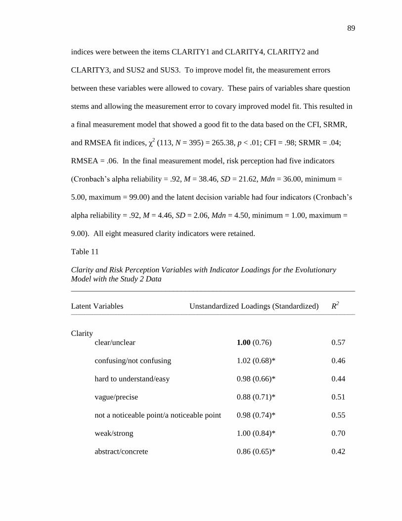
89

indices were between the items CLARITY1 and CLARITY4, CLARITY2 and

CLARITY3, and SUS2 and SUS3. To improve model fit, the measurement errors

between these variables were allowed to covary. These pairs of variables share question

stems and allowing the measurement error to covary improved model fit. This resulted in

a final measurement model that showed a good fit to the data based on the CFI, SRMR,

and RMSEA fit indices, χ2 (113, N = 395) = 265.38, p < .01; CFI = .98; SRMR = .04;

RMSEA = .06. In the final measurement model, risk perception had five indicators

(Cronbach‘s alpha reliability = .92, M = 38.46, SD = 21.62, Mdn = 36.00, minimum =

5.00, maximum = 99.00) and the latent decision variable had four indicators (Cronbach‘s

alpha reliability = .92, M = 4.46, SD = 2.06, Mdn = 4.50, minimum = 1.00, maximum =

9.00). All eight measured clarity indicators were retained.

Table 11

Clarity and Risk Perception Variables with Indicator Loadings for the Evolutionary

Model with the Study 2 Data

________________________________________________________________________


____________________________________________________________________________________________________________

Clarity



hard to understand/easy 0.98 (0.66)* 0.44

vague/precise 0.88 (0.71)* 0.51

not a noticeable point/a noticeable point 0.98 (0.74)* 0.55

weak/strong 1.00 (0.84)* 0.70

abstract/concrete 0.86 (0.65)* 0.42

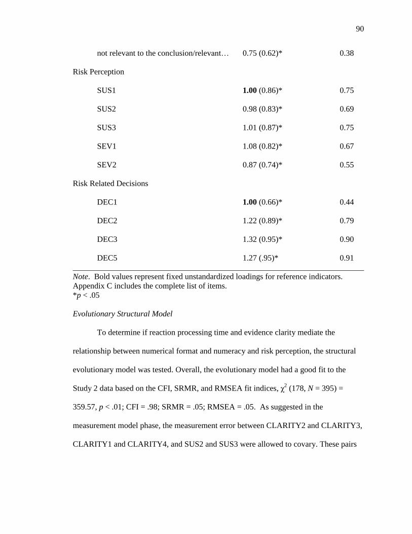
90

not relevant to the conclusion/relevant… 0.75 (0.62)* 0.38

Risk Perception

SUS1 1.00 (0.86)* 0.75

SUS2 0.98 (0.83)* 0.69

SUS3 1.01 (0.87)* 0.75

SEV1 1.08 (0.82)* 0.67

SEV2 0.87 (0.74)* 0.55


DEC1 1.00 (0.66)* 0.44

DEC2 1.22 (0.89)* 0.79

DEC3 1.32 (0.95)* 0.90

DEC5 1.27 (.95)* 0.91

________________________________________________________________________


Appendix C includes the complete list of items.

*p < .05

Evolutionary Structural Model

To determine if reaction processing time and evidence clarity mediate the

relationship between numerical format and numeracy and risk perception, the structural

evolutionary model was tested. Overall, the evolutionary model had a good fit to the

Study 2 data based on the CFI, SRMR, and RMSEA fit indices, χ2 (178, N = 395) =

359.57, p < .01; CFI = .98; SRMR = .05; RMSEA = .05. As suggested in the

measurement model phase, the measurement error between CLARITY2 and CLARITY3,

CLARITY1 and CLARITY4, and SUS2 and SUS3 were allowed to covary. These pairs

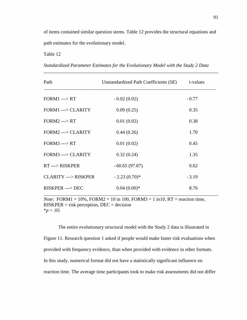
91

of items contained similar question stems. Table 12 provides the structural equations and

path estimates for the evolutionary model.

Table 12

Standardized Parameter Estimates for the Evolutionary Model with the Study 2 Data

________________________________________________________________________


_______________________________________________________________________

FORM1 ---> RT - 0.02 (0.02) - 0.77

FORM1 ---> CLARITY 0.09 (0.25) 0.35

FORM2 ---> RT 0.01 (0.02) 0.38

FORM2 ---> CLARITY 0.44 (0.26) 1.70

FORM3 ---> RT 0.01 (0.02) 0.45

FORM3 ---> CLARITY 0.32 (0.24) 1.35

RT ---> RISKPER - 60.65 (97.87) 0.62

CLARITY ---> RISKPER - 2.23 (0.70)* - 3.19

RISKPER ---> DEC 0.04 (0.00)* 8.76

________________________________________________________________________

Note: FORM1 = 10%, FORM2 = 10 in 100, FORM3 = 1 in10, RT = reaction time,

RISKPER = risk perception, DEC = decision

*p < .05

The entire evolutionary structural model with the Study 2 data is illustrated in

Figure 11. Research question 1 asked if people would make faster risk evaluations when

provided with frequency evidence, than when provided with evidence in other formats.

In this study, numerical format did not have a statistically significant influence on

reaction time. The average time participants took to make risk assessments did not differ

92

statistically between groups, F (3, 394) = 0.39, p > .05, η2 = 0.003. The means and

standard deviations for reaction time are provided in Table 13.

Table 13

Means and Standard Deviations for Reaction Time with the Study 2 Data

________________________________________________________________________

Numerical Format Mean Time in Milliseconds (SD)

________________________________________________________________________

Percent 7821.66 (3497.51)

Natural Frequency 8204.89 (3317.09)

Simple Frequency 8348.08 (5590.33)

Probability 7883.84 (3013.64)

________________________________________________________________________

Research question 2 asked: Will processing speed influence risk perception? The

results show that the path between reaction time and risk perception was not statistically

significant (β = -60.65, SE = 97.87, t = - 0.62). Reaction time did not have a statistically

significant influence on risk perception. Hypothesis 1 predicted that when risk

information was presented in a frequency format the evidence would be rated clearer than

when it was presented as a percentage or probability. Overall, no statistically significant

differences were found between the experimental conditions in regards to evidence

clarity. Table 12 shows that the paths between the experimental condition dummy

variables and the latent evidence clarity variable are not statistically significant.

Hypothesis 2 predicted that clarity would have a direct influence on risk perception. This

prediction was consistent with the data. Evidence clarity did have a direct, negative,

linear effect on risk perception in the model (β = -2.23, SE = 0.70, t = -3.19). Lower

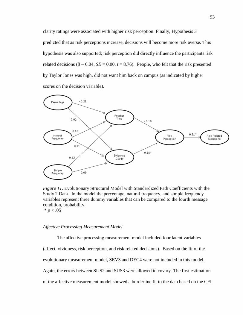
93

clarity ratings were associated with higher risk perception. Finally, Hypothesis 3

predicted that as risk perceptions increase, decisions will become more risk averse. This

hypothesis was also supported; risk perception did directly influence the participants risk

related decisions (β = 0.04, SE = 0.00, t = 8.76). People, who felt that the risk presented

by Taylor Jones was high, did not want him back on campus (as indicated by higher

scores on the decision variable).

Figure 11. Evolutionary Structural Model with Standardized Path Coefficients with the

Study 2 Data. In the model the percentage, natural frequency, and simple frequency



* p < .05

Affective Processing Measurement Model

The affective processing measurement model included four latent variables

(affect, vividness, risk perception, and risk related decisions). Based on the fit of the

evolutionary measurement model, SEV3 and DEC4 were not included in this model.

Again, the errors between SUS2 and SUS3 were allowed to covary. The first estimation

of the affective measurement model showed a borderline fit to the data based on the CFI

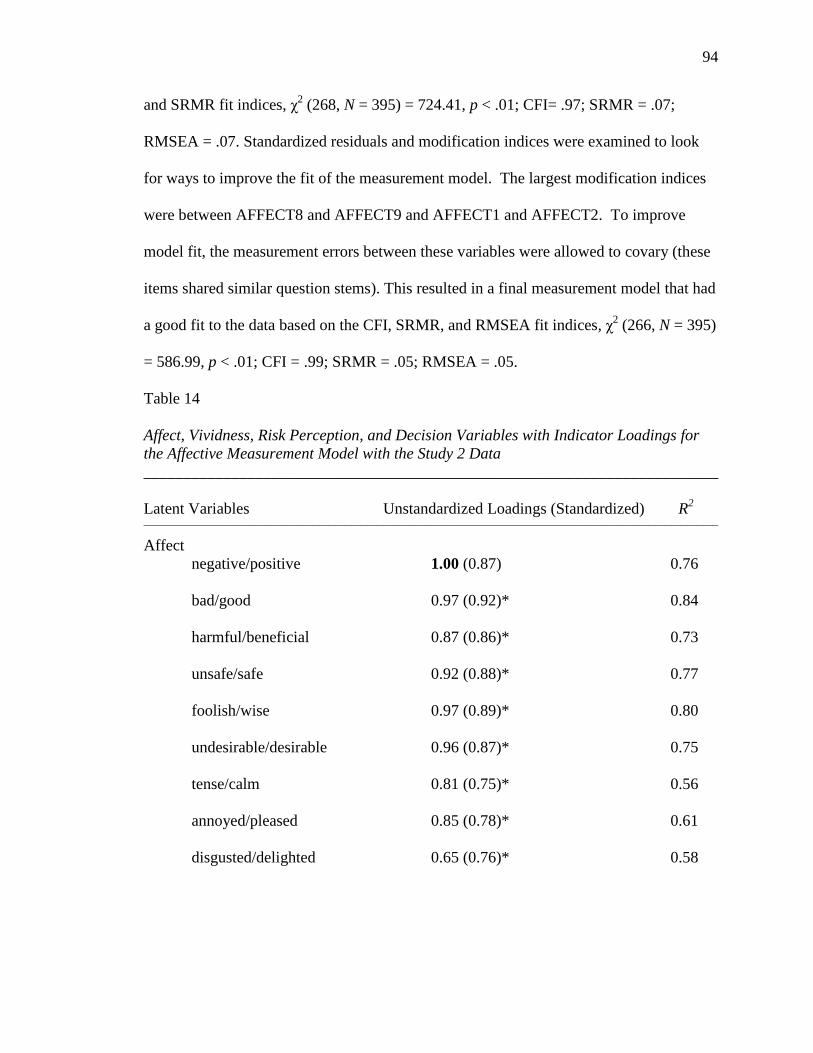
94

and SRMR fit indices, χ2 (268, N = 395) = 724.41, p < .01; CFI= .97; SRMR = .07;

RMSEA = .07. Standardized residuals and modification indices were examined to look

for ways to improve the fit of the measurement model. The largest modification indices

were between AFFECT8 and AFFECT9 and AFFECT1 and AFFECT2. To improve

model fit, the measurement errors between these variables were allowed to covary (these

items shared similar question stems). This resulted in a final measurement model that had

a good fit to the data based on the CFI, SRMR, and RMSEA fit indices, χ2 (266, N = 395)

= 586.99, p < .01; CFI = .99; SRMR = .05; RMSEA = .05.

Table 14

Affect, Vividness, Risk Perception, and Decision Variables with Indicator Loadings for

the Affective Measurement Model with the Study 2 Data

________________________________________________________________________


____________________________________________________________________________________________________________

Affect


bad/good 0.97 (0.92)* 0.84

harmful/beneficial 0.87 (0.86)* 0.73

unsafe/safe 0.92 (0.88)* 0.77

foolish/wise 0.97 (0.89)* 0.80


tense/calm 0.81 (0.75)* 0.56

annoyed/pleased 0.85 (0.78)* 0.61

disgusted/delighted 0.65 (0.76)* 0.58

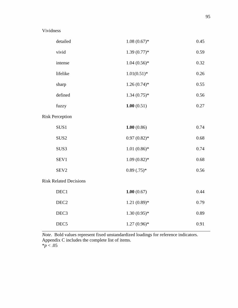
95

Vividness

detailed 1.08 (0.67)* 0.45

vivid 1.39 (0.77)* 0.59

intense 1.04 (0.56)* 0.32

lifelike 1.01(0.51)* 0.26

sharp 1.26 (0.74)* 0.55

defined 1.34 (0.75)* 0.56

fuzzy 1.00 (0.51) 0.27

Risk Perception

SUS1 1.00 (0.86) 0.74

SUS2 0.97 (0.82)* 0.68

SUS3 1.01 (0.86)* 0.74

SEV1 1.09 (0.82)* 0.68

SEV2 0.89 (.75)* 0.56


DEC1 1.00 (0.67) 0.44

DEC2 1.21 (0.89)* 0.79

DEC3 1.30 (0.95)* 0.89

DEC5 1.27 (0.96)* 0.91

________________________________________________________________________



*p < .05

96

Affective Processing Structural Model

To determine if affect and vividness mediate the relationship between the

exogenous variables numerical format and numeracy and the endogenous variables risk

perception and risk related decisions, the affective processing model was tested with the

Study 2 data. Based on the measurement phased, the measurement errors between SUS2

and SUS3, VIVIDNESS5 and VIVIDNESS6, and AFFECT8 and AFFECT9 were

allowed to covary. These pairs of items shared similar question stems. The affective

processing structural model had an acceptable fit to the data using the CFI and RMSEA

fit indices, χ2 (431, N = 395) = 1035.48, p < .01; CFI = .97; SRMR = .12; RMSEA = .06.

Table 15 provides the structural equations and path estimates.

Table 15

Standardized Parameter Estimates for the Affective Processing Model with the Study 2

Data

________________________________________________________________________


_______________________________________________________________________

FORM1 ---> RT - 0.01 (0.02) - 0.68

FORM1 ---> AFFECT - 0.19 (0.23) - 0.84

FORM1 ---> VIVIDNESS - 1.48 (2.40) - 0.62

FORM2 ---> RT 0.02 (0.02) 0.85

FORM2 ---> AFFECT - 0.28 (0.23) - 1.21

FORM2 ---> VIVIDNESS 3.11 (2.47) 1.26

FORM3 ---> RT 0.01 (0.02) 0.59

FORM3 ---> AFFECT - 0.06 (0.21) - 0.26

FORM3 ---> VIVIDNESS 2.32 (2.27) 1.02

97

ONUM ---> RT 0.02 (0.01)* 1.97

ONUM ---> AFFECT - 0.12 (0.10) - 1.19

ONUM ---> VIVIDNESS 0.58 (1.06) 0.55

SNUM ---> RT 0.00 (0.00) 0.34

SNUM ---> AFFECT 0.05 (0.06) 0.88

SNUM ---> VIVIDNESS 1.66 (0.67)* 2.47

FORMxONUM ---> RT 0.00 (0.00) - 0.70

FORMxONUM ---> AFFECT 0.02 (0.03) 0.51


RT ---> RISKPER - 93.13 (38.96)* - 2.39

AFFECT ---> RISKPER - 7.67 (0.66)* - 11.68

VIVIDNESS ---> RISKPER 0.10 (0.06) 1.65

RISKPER ---> DEC 0.04 (0.00)* 9.56

________________________________________________________________________

Note: FORM1 = 10%, FORM2 = 10 in 100, FORM3 = 1 in 10, RT = reaction time,

RISKPER = risk perception, DEC = decision, SNUM = subjective numeracy, ONUM =

objective numeracy, FORMxONUM = interaction term

*p < .05

The complete affective processing structural model is illustrated in Figure 12.

Hypothesis 4 predicted that numerical format would have a main effect on reaction time.

This prediction was not supported with the Study 2 data (Table 15 shows that the paths

between the numerical format dummy variables and reaction time are not statistically

significant). Hypothesis 5 predicted that numerical format would yield a main effect on

affect, such that frequency information would cause more negative affect in receivers

than information presented in other formats (percentages and probabilities). The paths

98

between the numerical format dummy variables and affect were not statistically

significant (see Table 15). Numerical format did not significantly influence affect as

predicted. Hypothesis 6 predicted that numerical format would yield a main effect on

vividness, such that frequency information would produce more vividness than

information presented in other formats (percentages and probabilities). Again, the paths

between the experimental formats and vividness were not statistically significant in the

model. Numerical format did not influence vividness as predicted by the model (see

Table 15). However, the thought listing data provides some support for this hypothesis.

Statistically significant differences between the experimental groups were found for

image intensity ratings, F (3, 383) = 2.80, p < .05, η2 = 0.02. A post hoc least squares

difference (LSD) test showed that the images reported by participants in the natural

frequency condition (10 in 100) were evaluated as more intense (M = 67.96, SD = 16.82)

than images in the percentage (10%) condition (M = 62.64, SD = 16.22, p < .05), the

simple frequency (1 in 10) condition (M = 62.76, SD = 16.65, p < 0.05 ), and the

probability (0.10 probability) condition (M = 60.52, SD = 20.34, p < .01). This is

consistent with the predictions of the affective processing theory. No statistically

significant between group differences existed between the experimental conditions for

positivity of the reported images (F (3, 385) = 0.58, p > .05, η2 = 0.002) or clarity of the

reported images (F (3, 387) = 0.59, p > .05, η2 = 0.002).

Hypothesis 7 predicted that numeracy would have a main effect on reaction time.

This hypothesis was supported by the data (β = 0.02, SE = 0.01, t = 1.97). The positive

path coefficient indicates that higher numeracy is associated with a longer response time.

ANOVA F-test results, using the objective numeracy median split variable, confirmed

99

this finding, F (1, 394) = 5.38, p < .05, η2 = 0.01. People with higher objective numeracy

(M = 8307.02, SD = 3230.22) spent more time making risk evaluations than participants

with lower objective numeracy (M = 7801.26, SD = 4786.89). This is consistent with the

literature. People with higher numeracy are more likely to spend time deliberating about

a risk, weighing the pros and cons. People with lower numeracy lack a clear

understanding of numbers and make faster, less deliberate evaluations. Preference for

numerical information did not have a statistically significant influence on reaction time

(see Table 15). Hypothesis 8 predicted that numeracy would yield a main effect on

affect, such that people with lower numeracy would experience more negative affect

from numerical information than people with higher numeracy. This hypothesis was not

supported for objective numeracy (β = - 0.12, SE = 0.10, t = - 0.26) or preference for

numerical information (β = 0.05, SE = 0.06, t = 0.88).

Hypothesis 9 predicted that numeracy would have a main effect on vividness,

such that people with higher numeracy would reported more vividness from numerical

information, than would people with lower numeracy. The path between objective

numeracy and vividness was not statistically significant; but, this hypothesis was

supported with the causal model for subjective numeracy data. Preference for information

influenced the amount of vividness reported (β = 1.66, SE = 0.67, t = 2.47). People who

prefer numerical information reported more vividness from the risk information in the

vignette.


influence reaction time. This prediction was not supported. The path between the

interaction term and reaction time was not statistically significant (β = 0.00, SE = 0.00, t

100

= - 0.70). Hypothesis 11 predicted that numerical format and numeracy would interact to

influence affect, such that people with lower numeracy will report more negative affect

from frequency information, compared to information presented in other numerical

formats. This hypothesis was also not supported. Numerical format and objective

numeracy did not interact to influence affect (β = 0.02, SE = 0.03, t = 0.51). Hypothesis

12 predicted that numerical format and objective numeracy would interact to influence

the amount of vividness reported, such that people with lower numeracy would report

more vividness from frequency information, compared to information presented in other

numerical formats. This prediction was not supported by the data (β = - 0.44, SE = 0.36, t

= - 1.22).

Hypothesis 13 predicted that reaction time would have a direct effect on risk

perception. This path was statistically significant (β = - 93.13, SE = 38.96, t = - 2.39).

Reaction time had a direct effect on risk perception. Longer (higher) response time was

associated with lower risk perception. People who took their time to evaluate the risk, had

lower risk perceptions than people who made quick, affective, System 2 evaluations.

Hypothesis 14 predicted that affect would influence risk perception, such that negative

affect would lead to higher perceived risk. This prediction was supported with the data (β

= -7.67, SE = 0.66, t = -11.66). As affect decreased (became more negative) risk

perception increased. Hypothesis 15 predicted that vividness would influence risk

perception, such that higher vividness would lead to higher risk perception. This

hypothesis was not supported (β = 0.10, SE = 0.06, t = 1.65). Hypothesis 16 predicted

that risk perception would influence risk related decisions. This hypothesis was supported

101

(β = 0.04, SE = 0.00, t = 9.56). Again, participants who evaluated the threat presented by

Taylor Jones as high did not want him back on campus (risk aversion).

Figure 12. Affective Processing Structural Model with Standardized Path Coefficients

with the Study 2 Data. In the model the percentage, natural frequency, and simple

frequency variables represent three dummy variables that can be compared to the fourth

message condition, probability

* p < .05

Integrated Measurement Model

The integrated measurement model included five latent variables (clarity, affect,

vividness, risk perception, and risk related decisions). Overall, the data had an acceptable

fit to the measurement model based on the CFI, SRMR, and RMSEA fit indices, χ2 (479,

N = 395) = 988.89, p < .01; CFI = .98; SRMR = .05; RMSEA = .05.

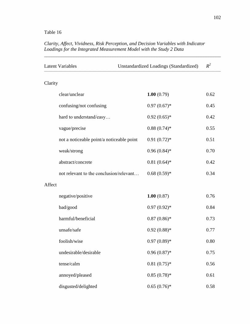
102

Table 16

Clarity, Affect, Vividness, Risk Perception, and Decision Variables with Indicator

Loadings for the Integrated Measurement Model with the Study 2 Data

________________________________________________________________________


____________________________________________________________________________________________________________

Clarity



hard to understand/easy… 0.92 (0.65)* 0.42

vague/precise 0.88 (0.74)* 0.55

not a noticeable point/a noticeable point 0.91 (0.72)* 0.51

weak/strong 0.96 (0.84)* 0.70

abstract/concrete 0.81 (0.64)* 0.42

not relevant to the conclusion/relevant… 0.68 (0.59)* 0.34

Affect


bad/good 0.97 (0.92)* 0.84

harmful/beneficial 0.87 (0.86)* 0.73

unsafe/safe 0.92 (0.88)* 0.77

foolish/wise 0.97 (0.89)* 0.80


tense/calm 0.81 (0.75)* 0.56

annoyed/pleased 0.85 (0.78)* 0.61

disgusted/delighted 0.65 (0.76)* 0.58

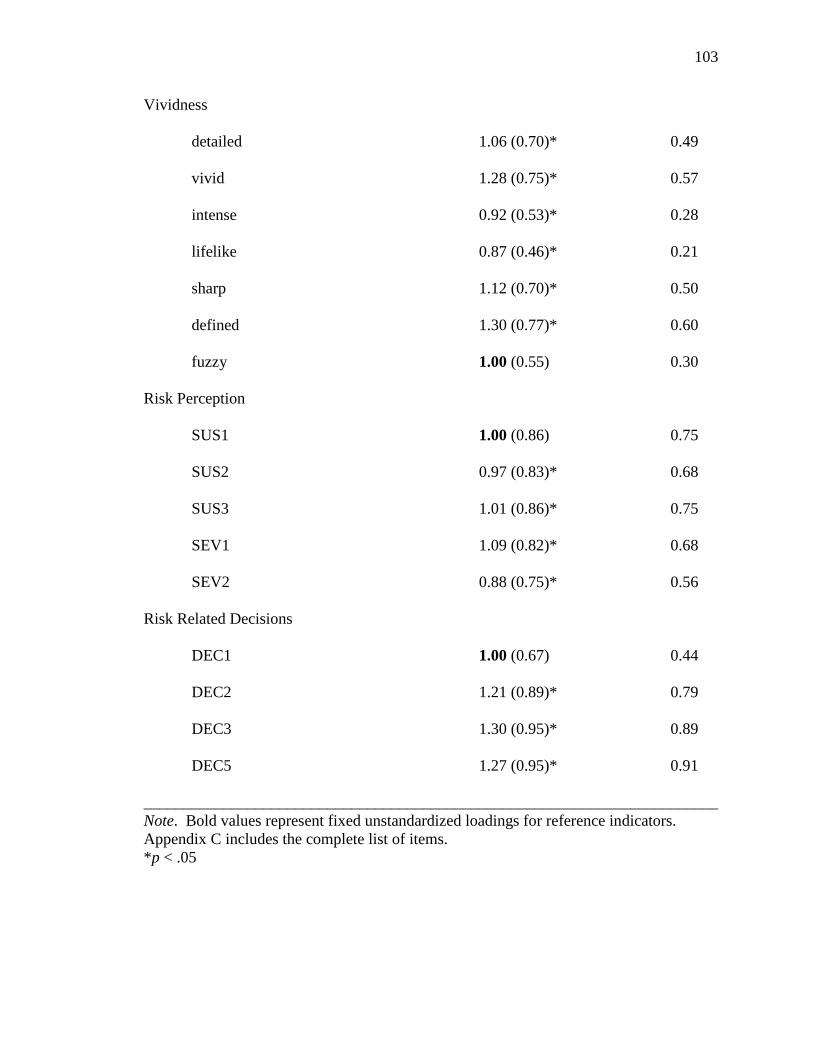
103

Vividness

detailed 1.06 (0.70)* 0.49

vivid 1.28 (0.75)* 0.57

intense 0.92 (0.53)* 0.28

lifelike 0.87 (0.46)* 0.21

sharp 1.12 (0.70)* 0.50

defined 1.30 (0.77)* 0.60

fuzzy 1.00 (0.55) 0.30

Risk Perception

SUS1 1.00 (0.86) 0.75

SUS2 0.97 (0.83)* 0.68

SUS3 1.01 (0.86)* 0.75

SEV1 1.09 (0.82)* 0.68

SEV2 0.88 (0.75)* 0.56


DEC1 1.00 (0.67) 0.44

DEC2 1.21 (0.89)* 0.79

DEC3 1.30 (0.95)* 0.89

DEC5 1.27 (0.95)* 0.91

________________________________________________________________________



*p < .05

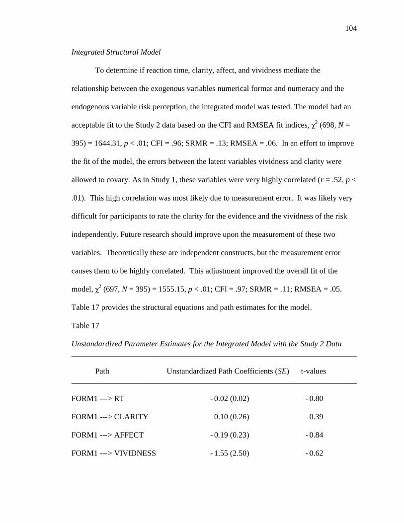
104

Integrated Structural Model

To determine if reaction time, clarity, affect, and vividness mediate the

relationship between the exogenous variables numerical format and numeracy and the

endogenous variable risk perception, the integrated model was tested. The model had an

acceptable fit to the Study 2 data based on the CFI and RMSEA fit indices, χ2 (698, N =

395) = 1644.31, p < .01; CFI = .96; SRMR = .13; RMSEA = .06. In an effort to improve

the fit of the model, the errors between the latent variables vividness and clarity were

allowed to covary. As in Study 1, these variables were very highly correlated (r = .52, p <

.01). This high correlation was most likely due to measurement error. It was likely very

difficult for participants to rate the clarity for the evidence and the vividness of the risk

independently. Future research should improve upon the measurement of these two

variables. Theoretically these are independent constructs, but the measurement error

causes them to be highly correlated. This adjustment improved the overall fit of the

model, χ2 (697, N = 395) = 1555.15, p < .01; CFI = .97; SRMR = .11; RMSEA = .05.

Table 17 provides the structural equations and path estimates for the model.

Table 17

Unstandardized Parameter Estimates for the Integrated Model with the Study 2 Data

________________________________________________________________________


________________________________________________________________________

FORM1 ---> RT - 0.02 (0.02) - 0.80

FORM1 ---> CLARITY 0.10 (0.26) 0.39

FORM1 ---> AFFECT - 0.19 (0.23) - 0.84

FORM1 ---> VIVIDNESS - 1.55 (2.50) - 0.62

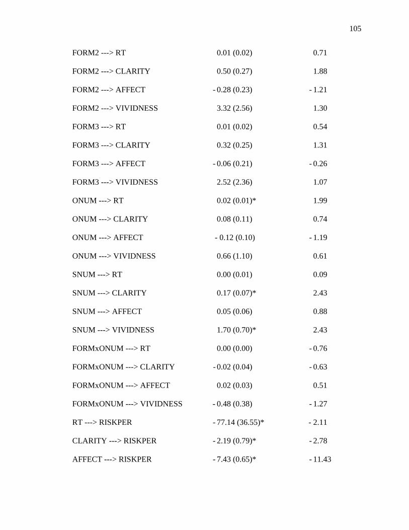
105

FORM2 ---> RT 0.01 (0.02) 0.71

FORM2 ---> CLARITY 0.50 (0.27) 1.88

FORM2 ---> AFFECT - 0.28 (0.23) - 1.21

FORM2 ---> VIVIDNESS 3.32 (2.56) 1.30

FORM3 ---> RT 0.01 (0.02) 0.54

FORM3 ---> CLARITY 0.32 (0.25) 1.31

FORM3 ---> AFFECT - 0.06 (0.21) - 0.26

FORM3 ---> VIVIDNESS 2.52 (2.36) 1.07

ONUM ---> RT 0.02 (0.01)* 1.99

ONUM ---> CLARITY 0.08 (0.11) 0.74

ONUM ---> AFFECT - 0.12 (0.10) - 1.19

ONUM ---> VIVIDNESS 0.66 (1.10) 0.61

SNUM ---> RT 0.00 (0.01) 0.09

SNUM ---> CLARITY 0.17 (0.07)* 2.43

SNUM ---> AFFECT 0.05 (0.06) 0.88

SNUM ---> VIVIDNESS 1.70 (0.70)* 2.43

FORMxONUM ---> RT 0.00 (0.00) - 0.76

FORMxONUM ---> CLARITY - 0.02 (0.04) - 0.63

FORMxONUM ---> AFFECT 0.02 (0.03) 0.51


RT ---> RISKPER - 77.14 (36.55)* - 2.11

CLARITY ---> RISKPER - 2.19 (0.79)* - 2.78

AFFECT ---> RISKPER - 7.43 (0.65)* - 11.43

106

VIVIDNESS ---> RISKPER 0.24 (0.09)* 2.79

RISKPER ---> DEC 0.04 (0.00)* 9.47

________________________________________________________________________

Note: FORM1 = 10%, FORM2 = 10 in 100, FORM3 = 1 in 10, RT = reaction time,

RISKPER = risk perception, DEC = decision, SNUM = subjective numeracy, ONUM =

objective numeracy, FORMxONUM = interaction term

*p < .05

Figure 13 presents the complete integrated structural model with the Study 2 data.

Hypothesis 17 predicted that numeracy would yield a main effect on clarity, such that

people with high numeracy would rate the numerical evidence as clearer than people with

low numeracy. Objective numeracy did not influence clarity ratings. However,

differences in preference for numerical information (subjective numeracy) were found.

The path between subjective numeracy and clarity was statistically significant in the

model (β = 0.17, SE = 0.07, t = 2.43). As preference for numerical information increased,

ratings of evidence clarity also increased.

Hypothesis 18 predicted that numerical format and objective numeracy would

interact to influence perceived evidence clarity, such that low numerate people would rate

evidence as clearer when it is presented in frequency formats; whereas, people with high

objective numeracy will have no clarity differences based on format. This hypothesis was

also not supported; the path from the interaction term to the evidence clarity variable was

not statistically significant (β = - 0.02, SE = 0.04, t = - 0.63).

In the integrated model, reaction time, clarity, affect, and vividness each had a

direct influence on risk perception. In the affective model, vividness was not a

statistically significant predictor of risk perception. In this model, clarity and vividness

were included at the same time and the errors between these variables were permitted to

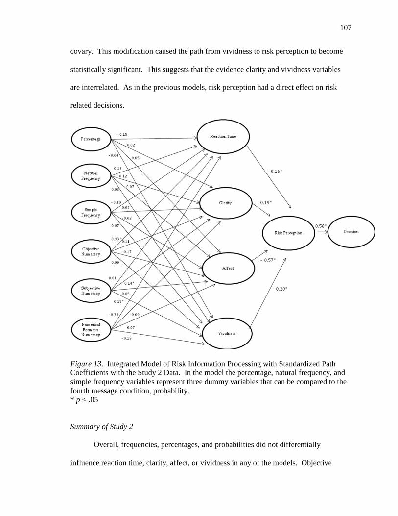
107

covary. This modification caused the path from vividness to risk perception to become

statistically significant. This suggests that the evidence clarity and vividness variables

are interrelated. As in the previous models, risk perception had a direct effect on risk

related decisions.

Figure 13. Integrated Model of Risk Information Processing with Standardized Path

Coefficients with the Study 2 Data. In the model the percentage, natural frequency, and

simple frequency variables represent three dummy variables that can be compared to the

fourth message condition, probability.

* p < .05

Summary of Study 2

Overall, frequencies, percentages, and probabilities did not differentially

influence reaction time, clarity, affect, or vividness in any of the models. Objective

108

numeracy had a main effect on reaction time and preference for numerical information

(subjective numeracy) had a direct influence on reported vividness and evaluations of

evidence clarity. Reaction time did not have any direct effects on risk perception in the

evolutionary model. But, when combined in the affective and integrated models, reaction

time did have a direct effect on risk perception. The mediating variables, reaction time,

clarity, affect, and vividness all directly influenced risk perception in the integrated

model. Also, in all three models, risk perception directly influenced risk related

decisions. As risk perception increased, people became more risk averse.

The three theories tested in Study 2 were compared using the Expected Cross-

Validation Index (ECVI). The evolutionary model, affective model, and integrated model

had ECVI indices of 1.18, 3.12, and 4.57 respectively. The model with the smallest

ECVI, the evolutionary model in this case, has the greatest potential for replication

(Byrne, 1998). The Akaike information criterion (AIC) is a second option for comparing

candidate models. The preferred model had the lowest AIC value. The evolutionary

model, affective model, and integrated model had AIC indices of 465.57, 1229.48, and

1640.00 respectively. Again, the evolutionary model is preferred. Notably, all three

models fit the data; but, the ECVI and AIC indices advocate for the more parsimonious

evolutionary model.

109

Chapter VII: Discussion

This chapter is separated into three parts. First, a summary of the results from

both studies is provided. This is followed by a discussion of the project‘s limitations and

finally the project‘s implications and directions for future research.

Summary of the Results

This dissertation project examined the variables that mediate the relationship

between the exogenous variables numerical presentation of risk information and

numeracy and the endogenous variables risk perception and risk related decisions.

Previous research suggested that numerical format and numeracy influence outcomes.

The question that remained unanswered was why? The goal of this project was peer into

the proverbial black box to critically examine information processing at work.

To examine possible mediating variables, two theoretical models that have

emerged in the risk perception literature were tested. The first was an evolutionary

model arguing that over time, human beings have developed an augmented ability to

process frequency information. Thus, frequency information is clearer and people are

faster at making decisions with information in this format. According to this model,

reaction time and evidence clarity mediate the relationship between numerical format and

risk perception. A second theoretical framework, the affective processing model, argued

that frequency information is more vivid and people can derive more affect from

information in this format. Therefore, according to this model, affect and vividness

mediate the relationship between evidence format and risk perception. In addition to

these two perspectives, a third model was also proposed and tested. The integrated model

of risk information processing predicted that the mediating variables reaction time,

110

clarity, vividness, and affect all influence risk perception. Two experiments were carried

out to test the predictions of these theories. These experiments were based on the work

of two teams of researchers that have been the principal advocates of the first two

theoretical perspectives.

The first goal of these two studies was to replicate the results found by Brase

(2002) and Slovic et al. (2000). Data from the two studies reported here support previous

findings. The data from Study 1 was able to replicate Brase‘s work that found statistically

significant differences between numerical formats on his one item clarity measure. In

addition, the data from Study 2 was used to replicate Slovic et al.‘s finding that numerical

format influenced risk perception. However, these two studies had flaws and limitations.

Brase measured clarity with one double barreled item and Slovic et al. measured risk

perception with one item on a three point scale. The two studies in this project aimed to

extend and elaborate upon previous research. First, this project made an effort to improve

the measurement of the latent variables of interest. Multiple items were used to measure

each latent variable and CFA procedures were used to assess the construct validity of

these measures. In addition, this project tested three theories that make predictions about

risk information processing. Three theoretical models were tested to explore the

mediating variables that influence risk perception.

When the mediating variables reaction time, clarity, affect, and vividness were

examined, Study 1 and Study 2 elicited a similar pattern of results. Numerical format did

not have a main effect on any of the mediating variables of interest in either study. In

both studies clarity, affect, and vividness had direct effects on risk perception. In all six

models, risk perception directly influenced risk related decisions. In Study 2, objective

111

numeracy had a main effect on reaction time, preference for numerical information

(subjective numeracy) had a direct effect on vividness and clarity, and reaction time had a

direct effect on risk perception in the affective and integrated models.

Limitations

Ecological Validity

First, the nature of the experiments and the sample of participants may have

affected the results of this study. This project included two lab experiments with a

sample of college age students. Lab studies allowed for experimental control. But, this

control came at a cost. Lab studies like this one lack mundane realism. When people are

presented with risk information in real world situations they feel differently than when

they are presented with a hypothetical risk in the lab.

Another concern is related to one of the main variables of interest, objective

numeracy. Collecting data with an educated sample of college students limited the

variance in numeracy. Few participants received very low scores on this scale. This is a

global limitation of numeracy research; this variable has been studied largely in educated

populations. To date, there is very little data available regarding how people with low

numeracy respond to and use quantitative risk information. In addition, numeracy can be

studied in conjunction with other individual differences that are related to the

comprehension and processing of numerical information. These individual differences

may include math anxiety or math dyslexia.

Study Design

Some limitations to the study design have been identified. First, future research

should make an effort to design messages that sound like real newspaper headlines, if this

112

medium is provided as the context for the evidence. As written, the Brase messages do

not read like newspaper headlines. This may have influenced the evaluation of the

messages in this study.

In addition, personal involvement may be one cause of the difference in results

between the two main studies. In Study 1, participants were given short messages. These

messages were not particularly involving. In Study 2, participants were given a longer

message, a hypothetical vignette. The vignette was about a student at the participants‘

own University. This topic should be more personally and emotionally relevant to the

participants. Therefore, the differences between the two studies may be caused by the

messages and topics. For example, no interaction effects between format and numeracy

were found for affect in Study 2. It is plausible that the more involving violent student

topic caused more negative affect regardless of the numerical presentation format. In

Study 1, participants did not report strong affect overall. Only two of the eight observed

variables (negative and undesirable) were strong predictors of the latent affect variable.

In contrast, all seven observed variables were strong indicators of affect in Study 2.

In addition to involvement, the comments provided by participants in Study 1

identified another concern. Several participants mentioned that they quickly read the

headline with the evidence, not realizing that they would be asked questions about it later.

The headline did appear again half way through the study, but this did not help

participants answer the questions that immediately followed the original message. To

minimize this concern, at the start of Study 2 participants were instructed that they would

be asked questions about the vignette and once they move forward, the computer program

113

will not allow them to go back. The addition of this reminder could be one cause of the

differences between the two studies.

Finally, one possible explanation for the lack of differences between the

experimental groups, on the mediating variables of interest, may be because it was too

difficult for participants to evaluate the numerical evidence. It is challenging to decide if

a piece of evidence is clear or vivid when it is received in isolation. Future research

could have participants make comparisons, as opposed to evaluating only one message at

a time. Perhaps by asking participants, ―is .10 easier to understand than 10 out of 100‖ or

―is 1 in 10 easier to imagine than 10%‖, researchers can more adequately assess the

differences between numerical formats. Alternatively, definitions of the terms being used

could be provided. This final concern is related to another set of limitations involving the

measurement of the dependent variables.

Measures of the Dependent Variables

As discussed previously, the measurement of the dependent variables may have

affected the results. In general, the observed measures were stronger indicators of the

latent mediating variables in Study 2 than in Study 1. This may have been caused by

participants rushing through the headline, as previously mentioned. Another possible

cause may be the topic of Study 2. The topic may have been more interesting and

involving to the participants causing them to take more time to complete the measures of

the dependent variables. Perhaps a risk that could exist on the participants‘ own campus

was truly more affective, vivid, or clear.

This study improved upon the single item measures employed by Brase (2002)

and Slovic et al. (2000), but measurement of the variables of interest can continually be

114

improved upon. For example, affect was measured with nine items focused on evaluating

positive or negative feelings. Including a more comprehensive measure of affect that

includes discrete emotions could be useful. The Positive Affect Negative Affect

Schedule (PANAS) is one example of a more comprehensive measure (Watson, Clark, &

Tellegen, 1988). This scale measures 11 specific emotions: fear, sadness, guilt, hostility,

shyness, fatigue, surprise, joviality, self-assurance, attentiveness, and serenity.

Finally, the risk perception measures could be expanded in future research. In

these studies risk susceptibility and risk severity were measured with six items. These

items were general in nature and did not measure specific risk factors (e.g., ―how likely is

Taylor Jones to commit another act of violence?‖). More specific items could distinguish

between different aspects of a risk. For example, in Study 2 more specific risk

susceptibility measures could include: how likely is Taylor Jones to commit another act

of violence on campus?; how likely is Taylor Jones to commit another act of violence off

campus?; and how likely are you to be a victim of Taylor Jones?

Exclusion of a Control Group

The inclusion of a control group may have assisted in the interpretation of the

results in this project. If each study included a fifth message condition that contained no

numerical evidence, the effects of numerical evidence in general on the mediating

variables of interest may have been clarified. It could be useful to compare the effects of

numerical evidence to the effects of no evidence. From a data analysis standpoint, this

control group could serve as the comparison group in the MIMIC procedure that was

used in this project.

115

Implications and Future Research Directions

Theoretical Implications

Numerical format did not directly influence any of the mediating variables

suggested by the evolutionary model or the affective processing model. Although one

might conclude that no variables mediate the relationships between numerical format and

risk perception, these data provide some evidence against this stance. When the

mediating variables were removed from the models, neither numerical format nor

numeracy had statistically significant direct effects on risk perception or risk related

decisions. Therefore, a second conclusion may be that there are other mediating variables

that have not been included in the model. Possible mediating variables may include

discrete emotions rather than positive or negative affect. Discrete emotions were not

included in the predictions of the two theories tested in this project; but, the effects of

discrete emotions on risk perception have been well documented. For example, Lerner

and Keltner (2000) found that fear and anger have opposite effects on risk perception.

When experiencing fear, people have pessimistic risk estimates and are more risk averse

in their decision making. In contrast, angry people make more optimistic risk evaluations

and are more risk seeking in their choices.

Future research projects should work toward the development of message design

theory. There continues to be a lack of theory in the field of communication focused on

message design features. This project focused on one message design feature, numerical

format. Beyond numerical format, there is a multitude of other ways to present risk

information. Risk information can be presented without numbers, using verbal labels

such as rarely or often. A risk can be described with qualitative evidence, such as a

116

testimony or a narrative. Risk information can also be presented visually with pictures,

graphs, or icons. These formats need to be systematically tested as well. It is plausible

that formats (e.g., qualitative, quantitative, graphical) may have differential effects on the

mediating variables hypothesized in the theoretical models. The integrated model can be

expanded to include various formats of risk information (see Figure 14).

Figure 14. Expanded Integrated Theory of Risk Information Processing

Previous research had documented the differential effects of presentation format.

For example, Tait, Voepel-Lewis, Zikmund-Fisher, and Fagerlin (2010) randomized

participants to receive information about risks using text, tables, or pictographs. The

authors found that tables and pictographs led to increased comprehension, compared to

standard text. It is possible that visual information has differential effects on reaction

117

time, clarity, affect, and vividness as well. The inclusion of other presentation formats

would make for a wide ranging theory that makes predictions about the effects of

evidence presentation on risk perception.

Finally, in addition to numeracy, other individual differences may influence the

mediating variables of interest. Involvement, personal control, and personal experiences

may serve as a lens through which risk information is evaluated.

Applied Implications

In addition to theory building, the results of this research also have applied

implications. Preference for information (subjective numeracy) was a statistically

significant predictor of perceived evidence clarity and perceived vividness of the risk.

This variable is correlated with objective numeracy in the literature and these variables

were correlated in this project as well. Risk communicators often must provide

numerical information to a patient about a risk. That risk may be side effect of a

medication the patient is being prescribed, a treatment option for a diagnosed disease, the

risks of lifestyle factors, or the results of genetic testing. A subjective numeracy measure

could provide feedback to communicators regarding how to best communicate risk to a

patient. This measure can also serve as a proxy for objective numeracy in situations

where fast feedback is needed or an objective test is not feasible. A short version of the

13-item subjective numeracy scale could be useful in patient-provider interactions. A

CFA of the entire 13-item subjective numeracy scale showed that three items are the

strongest indictors of the latent preference for numerical information variable. By asking

a patient three questions (how good are you at working with fractions?, how good are you

at working with percentages?, and when reading a newspaper, how helpful do you find

118

tables and graphs that are part of a story?) a health care provider can quickly assess a

patient‘s numeracy. Based on this information, messages can quickly and easily be

tailored to a patient‘s needs and personal preferences.

Future work in this area can take an applied direction as well. There is still an

unanswered question involving real direct effects on decision making. This study, like

most of the work that came before, asked people to report about their susceptibility for

and the severity of a hypothetical risk. In addition, participants were asked what they

would do in a risk situation or how much money they would donate. The question that

remains is: can these findings be translated into actual behavior, not only behavioral

intention? This is an enormous unanswered question that could have a tremendous

amount of practical value.

Conclusion

This project was an initial effort to test variables that have been predicted to

mediate the processing of quantitative risk evidence. This project worked toward finding

an answer to the question: why does numerical format and numeracy influence risk

perception? Although numerical format did not influence the predicted mediating

variables differentially, the hypothesized mediating variables did have consistent and

direct effects on risk perception. As predicted in this model, reaction time, clarity, affect,

and vividness had direct effects on risk perception. And, risk perception had a strong

influence on risk related decisions. This last finding was consistent across three risk

topics: disease prevalence, drug efficacy, and campus safety. In addition, this project

provided evidence for the prediction that people with high numeracy will spend more

time evaluating a risk when given numerical information.

119

For the first time, two theories of risk information processing, an evolutionary

theory and an affective processing theory, were depicted as causal models. Testing these

theories in their entirely is the only way to develop and extend these models. Support

was found for all three theories, including the integrated theory of risk information

processing that was proposed in this project for the first time. Overall, the results of this

project support the prediction that the evolutionary theory and the affective processing

theory are not competing perspectives. The integrated theory of risk information

processing can continue to be developed as work in this area moves forward.

120

Endnotes

1. Risk has been defined in other ways. Yates and Stone (1992) defined risk as the

possibility of loss. Oglethorpe and Monroe (1994) defined risk as probability times

outcome.

2. Risk perception has been defined in other ways in the literature. Slovic (1987) defined

risk perceptions as intuitive risk judgments. Oglethorpe and Monroe (1994) suggested

that the perception of risk is comprised of some combination of the probability of a

negative outcome and severity of that outcome. Perceived risk is defined as an

individual's subjective belief that there is some probability that an undesired outcome will

result from a choice. That is, there is some nonzero chance that any given choice may

lead to an undesired result or outcome.

3. In the original Slovic et al. (2000) study, only two formats, frequencies and

percentages, were compared. Four formats (natural frequencies, simple frequencies,

probabilities, and percentages) will be compared in this study.

121

Appendix A

Pilot Study Survey Instrument

Risk Situations Survey

Thank you for participating in this research study. You will complete two sets of

questions. Please do your best to answer every question.

Instructions: You will read three short risk situations. Please read each situation and

answer the questions that follow.

Situation 1

A student, Taylor Jones, was expelled from the University of Maryland last year for

committing a violent act. Jones has been treated for the past several weeks at an acute

civil mental health facility and has been evaluated for discharge. A psychologist has

done a state-of-the art assessment of Jones. Among the conclusions reached in the

psychologist‘s assessment is the following:

Patients similar to Jones are estimated to have a 10% probability of committing an act of

violence to others during the first several months of discharge.

Currently, Jones has applied to be re-admitted to the University of Maryland. This

application is currently being evaluated.

1. Do you think this situation is realistic? (0 = not realistic at all, 9= completely realistic)

2. Please explain why you think this situation is realistic or not realistic.

3. What could be added or removed to make this situation more realistic?

4. Do you think Taylor Jones is: male female

5. Is Taylor typically man‘s name or a woman‘s name? man woman

6. Is this scenario clear as it is written?

7. Is anything confusing or unclear about this scenario? Be specific.

8. If this situation was happening at UMD, how would you feel?

9. How much do you care about Jones attending UMD? (0 = I do not care if Jones

returns to UMD or not, 9 = I care a great deal if Jones returns to UMD).

Situation 2

It is estimated that by the year 2020, 1% of all Americans will have been exposed to a

new flu strain X.

1. Do you think this situation is realistic? (0 = not realistic at all, 9 = completely

realistic)



4. Is this information clear as it is written?

5. Is anything confusing or unclear about this information? Be specific.

6. How does this information make you feel?

122

7. How much do you care about flu strain X? (0 = I do not care at all, 9 = I care a great

deal)

Situation 3

A new drug is about to be approved by the FDA. It has been estimated to cause negative

side effects in 99% of all Americans.

1. Do you think this situation is realistic? (0 = not realistic at all, 9= completely realistic)



4. Is this information clear as it is written?

5. Is anything confusing or unclear about this information? Be specific.

6. How does the pending approval of this new drug make you feel?

7. How much do you care about the approval of this new drug? (0 = I do not care at all, 9

= I care a great deal)

Instructions: In this final set of questions, we would like to get some general information

about you.

1. What is your sex? male female

2. Which of the following best describes your race? Please mark all that apply.

African-American or Black

Hispanic or Latino

Asian-American

Native American

Caucasian or White

Other. Please specify _____________

3. What year are you in at school?

Freshman

Sophomore

Junior

Senior

Graduate Student

Other. Please specify

4. How old are you? ____________ years old

5. Do you have any questions or comments about this survey?

Thank you for completing all questions. We appreciate your participation

in this research study. The information you just read is fictitious and does not refer to

any real UMD students, flu strains, or new drugs.

123

Appendix B

Study 1 Experiment Protocol

Welcome. Thank you for participating in this research study. Press any key to begin.

For this research study, you will read a recent New York Times newspaper headline.

Using the information in the headline, you will be asked to answer several questions. You

will answer some questions by using your computer keyboard. Other questions will ask

you to provide answers by using the button box that is attached to your computer. For

each question, you will be instructed to use the keyboard or the button box. Press any

key to continue.

Instructions: In a minute, a series of questions will appear on your computer screen.

Some questions will ask you to answer by using the computer keyboard. Other questions

will ask you to use the button box that is attached to your computer. Let‘s practice using

both. Press any key to continue.

Press 1 on the button box.

Enter the number 10 using the keyboard.

Please use the button box to answer the following question. How much do you like

chocolate ice cream? (1 = not at all, 9 = very much)

Let‘s begin. Press any key to continue.

The following information is a recent New York Times newspaper headline.

It is estimated that by the year 2020, any given American will have a probability of 0.01

of having been exposed to Flu strain X.

Press any key to continue.

What year was mentioned in the headline you just read? Please type a year using the

keyboard. If no year was mentioned type, ―no year‖.

BRASEclarity. How clear and easy to understand is the statistical information presented

in the headline? (1 = unclear, 9 = clear)

DEC1(disease prevalence). If you were in charge of the annual budget for the U.S.

Department of Health, how much of every $100 in the budget would you dedicate to

dealing with Flu strain X? Using your keyboard please enter a value between 0 and 100.

DEC1(drug efficacy). If you were in charge of the production budget for the

manufacturer of this drug, how much of every $100 would you dedicate to producing this

drug? Using the keyboard, enter a number between 0 and 100.

124

(thought listing items)

Instructions: We have images and ideas about things. Often when people hear about a

particular risk, they develop images in their minds about the meaning of the risk. We are

interested in the meaning of certain risks to people like you. Think for a moment about

the [the flu/the drug] in the headline you just read. We are interested in the first five

images that come to your mind when you think about [the flu/the drug] in the headline.

Think about five images now and write them down on your paper. When you are done

writing, press any key to continue.

Please list your five images.

1. ______________________________________________________________

2. _____________________________________________________________

3. _____________________________________________________________

4. ______________________________________________________________

5. ______________________________________________________________

Now that you have thought about and listed five images that come to mind when you

think about [the flu/the drug] in the headline, we want to be sure that we understand what

these images mean to you. Remember, we are asking you to evaluate your five images,

not the headline. Press any key to continue.

From your list, type your first image.

Using a scale from 0-100, how positive is your first image (0 = completely negative and

100 = completely positive)? Type a number from 0 – 100 using the keyboard.

Using a scale from 0-100, how clear is your first image (0 = completely fuzzy and 100 =

completely clear)? Type a number from 0 – 100 using the keyboard.

Using a scale from 0-100, how intense is your first image (0 = weak and 100 = strong)?

Type a number from 0 – 100 using the keyboard

From your list, type your second image.

Using a scale from 0-100, how positive is your second image (0 = completely negative

and 100 = completely positive)? Type a number from 0 – 100 using the keyboard.

Using a scale from 0-100, how clear is your second image (0 = completely fuzzy and 100

= completely clear)? Type a number from 0 – 100 using the keyboard.

Using a scale from 0-100, how intense is your second image (0 = weak and 100 = strong)


125

From your list, type your third image.

Using a scale from 0-100, how positive is your third image (0 = completely negative and


Using a scale from 0-100, how clear is your third image (0 = completely fuzzy and 100 =


Using a scale from 0-100, how intense is your third image (0 = weak and 100 = strong)?


From your list, type your fourth image.

Using a scale from 0-100, how positive is your fourth image (0 = completely negative


Using a scale from 0-100, how clear is your fourth image (0 = completely fuzzy and 100


Using a scale from 0-100, how intense is your fourth image (0 = weak and 100 = strong)?

Type a number from 0 – 100 using the keyboard.

From your list, type your fifth and final image.

Using a scale from 0-100, how positive is your fifth image (0 = completely negative and


Using a scale from 0-100, how clear is your fifth image (0 = completely fuzzy and 100 =


Using a scale from 0-100, how intense is your fifth image (0 = weak and 100 = strong)?


For this next set of questions, use the button box attached to your computer.

DEC2(disease prevalence). If a vaccination for Flu strain X was available, how likely

would you be to get it? (1= not likely at all, 9 = very likely)

DEC3(disease prevalence). How closely should the U.S. government monitor Flu strain

X? (1= not closely at all, 9 = very closely).

DEC2(drug efficacy). How likely would you be to take the drug in the headline if it was

prescribed to you? (1= not likely at all, 9 = very likely)

DEC3(drug efficacy). How closely would you want the FDA to monitor the drug in the

headline after it is approved? (1= not closely at all, 9 = very closely).

(vividness items)

This next set of questions will ask you how vivid the risk in the headline is to you.

Remember the headline is: (evidence manipulation). Press any key to continue.

126

VIVIDNESS1. How FUZZY is the risk being described? Using a scale from 0 (not fuzzy

at all) to 100 (extremely fuzzy) enter a number from 0 to 100 using the keyboard.

VIVIDNESS2. How DETAILED is the risk being described? Using a scale from 0 (not

detailed at all) to 100 (extremely detailed) enter a number from 0 to 100 using the

keyboard.

VIVIDNESS3. How VIVID is the risk being described? Using a scale from 0 (not vivid

at all) to 100 (extremely vivid) enter a number from 0 to 100 using the keyboard.

VIVIDNESS4. How INTENSE is the risk being described? Using a scale from 0 (not

intense at all) to 100 (extremely intense) enter a number from 0 to 100 using the

keyboard.

VIVIDNESS5. How LIFELIKE is the risk being described? Using a scale from 0 (not

lifelike at all) to 100 (extremely lifelike) enter a number from 0 to 100 using the

keyboard.

VIVIDNESS6. How SHARP is the risk being described? Using a scale from 0 (not sharp

at all) to 100 (extremely sharp) enter a number from 0 to 100 using the keyboard.

VIVIDNESS7. How WELL-DEFINED is the risk being described? Using a scale from 0

(not defined at all) to 100 (extremely well-defined) enter a number from 0 to 100 using

the keyboard.

(affect items)

For this next set of questions, we are interested in learning about how the risk makes you

feel. Please use the button box to respond to the next set of questions. Press any key to

begin this set of questions.

Flu strain X is/The side effects of the drug in the headline are:

AFFECT1 negative 1 2 3 4 5 6 7 8 9 positive

AFFECT2 bad 1 2 3 4 5 6 7 8 9 good

AFFECT3 harmful 1 2 3 4 5 6 7 8 9 beneficial

AFFECT4 unsafe 1 2 3 4 5 6 7 8 9 safe

Dedicating resources to deal with Flu strain X is/The drug in the headline is:

AFFECT5 foolish 1 2 3 4 5 6 7 8 9 wise

AFFECT6 undesirable 1 2 3 4 5 6 7 8 9 desirable

127

Dedicating resources to deal with Flu strain X is/Dedicating resources to the testing of the

drug in the headline:

AFFECT7 makes me

feel tense

1 2 3 4 5 6 7 8 9 makes me

feel calm

AFFECT8 make me

feel

annoyed

1 2 3 4 5 6 7 8 9 makes me

feel pleased

AFFECT9 makes me

feel

disgusted

1 2 3 4 5 6 7 8 9 makes me

feel

delighted

(evidence clarity items)

For the next set of questions, please evaluate the headline you just read. Use the button

box for this set of questions. Press any key to continue.

The information in the headline is:

CLARITY1 unclear 1 2 3 4 5 6 7 8 9 clear

CLARITY2 confusing 1 2 3 4 5 6 7 8 9 not

confusing

CLARITY3 hard to

understand

1 2 3 4 5 6 7 8 9 easy to

understand

CLARITY4 vague 1 2 3 4 5 6 7 8 9 Precise

CLARITY5 not a

noticeable

point

1 2 3 4 5 6 7 8 9 a noticeable

point

CLARITY6 weak 1 2 3 4 5 6 7 8 9 strong

CLARITY7 abstract 1 2 3 4 5 6 7 8 9 concrete

CLARITY8 not relevant

to the

conclusion

1 2 3 4 5 6 7 8 9 relevant to

the

conclusion

(risk perception items)

This next set of questions will ask you how you feel about the risk in the headline. Use

the keyboard to type your answers. Press any key when you are ready to begin.

(perceived susceptibility items)

Using a scale from 0 (impossible to happen) to 100 (certain to happen)

128

(disease prevalence)

SUS1. Using a scale from 0 (impossible to happen) to 100 (certain to happen) how

certain are you that you will be exposed to flu strain X?

SUS2. Using a scale from 0 (impossible to happen) to 100 (certain to happen) what is the

chance that you will be exposed to flu strain X?

SUS3. Using a scale from 0 (impossible to happen) to 100 (certain to happen) how likely

is it that you will be exposed to Flu strain X?

(drug efficacy)

SUS1. Using a scale from 0 (impossible to happen) to 100 (certain to happen) how

certain are you that you will experience negative side effects if you take the drug in the

headline?

SUS2. Using a scale from 0 (impossible to happen) to 100 (certain to happen) what is the

chance that you will experience negative side effects if you take the drug in the headline?

SUS3. Using a scale from 0 (impossible to happen) to 100 (certain to happen) how likely

is it that you will be experience side effects if you take the drug in the headline?

(perceived severity items)

Using a scale from 0 (no risk) to 100 (high risk)

(disease prevalence)

SEV1. Using a scale from 0 (impossible to happen) to 100 (certain to happen) what is the

risk of being exposed to Flu strain X?

SEV2. Using a scale from 0 (impossible to happen) to 100 (certain to happen) how

dangerous is Flu strain X?


serious is the existence of Flu strain X?

(drug efficacy)


risk of experiencing negative side effects if you take the drug in the headline?


risk if the FDA approves the drug in the headline?


serious are the negative side effects of the drug in the headline?

(objective numeracy items)

For this next set of questions, read each question and use the keyboard to provide an

answer. Use the scratch paper next to your computer if you need it. Press any key to

begin.

ONUM1. Which of the following numbers represents the biggest risk of getting a

disease? 1 in 100, 1 in 1,000, or 1 in 10? Please type your answer using the keyboard.

(Answer: 1 in 10)

ONUM2. Which of the following represents the biggest risk of getting a disease: 1%,

10%, or 5%? Please type your answer using the keyboard. (Answer: 10%)

129

ONUM3. If the chance of getting a disease is 10%, how many people would be expected

to get the disease out of 100? Please type your answer using the keyboard. (Answer: 10)


to get the disease out of 1,000? Please type your answer using the keyboard. (Answer:

100)

ONUM5. If the chance of getting a disease is 20 out of 100, this would be the same as

having a ___% chance of getting the disease. Please type your answer using the

keyboard. (Answer: 20%)

ONUM6. If person A‘s chance of getting a disease is 1% in 10 years, and person B‘s risk

is double that of A‘s, what is B‘s risk? Please type your answer using the keyboard.

(Answer: 2% in 10 years; 2 in 10; 1 in 5)

ONUM7. If person A‘s chance of getting a disease is 1 in 100 in 10 years, and person B‘s

risk is double that of A‘s, what is B‘s risk? Please type your answer using the keyboard.

(Answer: 2; 2 in 100; 1 in 50 in 10 years)

ONUM8. In the Big Bucks Lottery, the chances of winning a $10.00 prize are 1%. What

is your best guess about how many people would win a $10.00 prize if 1000 people each

buy a single ticket from Big Bucks? Please type your answer using the keyboard.

(Answer: 10)

ONUM9. Imagine that we roll a fair six-sided die 1000 times. Out of 1000 rolls, how

many times do you think the die would come up as an even number (2, 4, or 6)? Please

type your answer using the keyboard. (Answer: half the time; 50%; 500; 1:2)

ONUM10. The chance of getting a viral infection is .0005. Out of 10,000 people, about

how many of them are expected to get infected? Please type your answer using the

keyboard. (Answer: 5)

ONUM11. In the Acme Publishing Sweepstakes, the chances of winning a car is 1 in

1,000. What percent of tickets in Acme Publishing Sweepstakes win a car? Please type

your answer using the keyboard. (Answer: .10; 1%)


disease? 1 chance in 12 or 1 chance in 37. Please type your answer using the keyboard.

(Answer: 1 chance in 12)

130

ONUM13. Suppose you have a close friend who has a lump in her breast and must have a

mammography. Of 100 women like her, 10 of them actually have a malignant tumor and

90 of them do not. Of the 10 women who actually have a tumor, the mammography

indicates correctly that 9 of them have a tumor and indicates incorrectly that 1 of them

does not have a tumor. Of the 90 women who do not have a tumor, the mammography

indicates correctly that 81 of them do not have a tumor and indicates incorrectly that 9 of

them do have a tumor. Imagine that your friend test positive (as if she had a tumor).

What is the likelihood that she actually has a tumor? Please type your answer using the

keyboard. (Answer: 9 out of 18; 1 out of 2; 50%; 1:2)

ONUM14. Imagine that you are taking a class and your chances of being asked a

question in class are 1% during the first week of class and double each week thereafter

(i.e., you would have a 2% chance in Week 2, a 4% chance in week 3, and 8% chance in

week 4). What is the probability that you will be asked a question in class during week

7? Please type your answer using the keyboard. (Answer: 64%)

ONUM15. Suppose that 1 out of every 10,000 doctors in a certain regimen is infected

with the SARS virus; in the same region, 20 out of every 100 people in a particular at-risk

population are also infected with the virus. A test for the virus gives a positive result in

99% of those who are infected and in 1% of those who are not infected. A randomly

selected doctor and a randomly selected person in the at-risk population in this region

both test positive for the disease. Who is more likely to actually have the disease? Please

type A, B, or C using your keyboard. (Answer: C)

A. They both tested positive for SARS and therefore are equally likely to have the disease

B. They both tested positive for SARS and the doctor is more likely to have the disease

C. They both tested positive for SARS and the person in the at-risk population is more

likely to have the disease

(subjective numeracy items)

For this set of questions, please choose one response using the 1-9 scale on your button

box. Press any key to begin.

SNUM1. How good are you at working with fractions? (1 = not good at all, 9 =

extremely good)

SNUM2. How good are you at working with percentages? (1 = not good at all, 9 =

extremely good)

SNUM3. How good are you at calculating a 15% tip on a bill? (1 = not good at all, 9 =

extremely good)

SNUM4. How good are you at figuring out how much a shirt will cost if it is marked

25% off? (1 = not good at all, 9 = extremely good)

131

SNUM5. When reading the newspaper, how helpful do you find tables and graphs that

are part of a story? (1 = not helpful at all, 9 = extremely helpful)

SNUM6. When people tell you the chance of something happening, do you prefer that

they use words (―it rarely happens‖) or numbers (―there is a 1% chance‖)? (1 = always

prefer words, 9 = always prefer numbers)

SNUM7. When you hear a weather forecast, do you prefer predictions using percentages

(―there will be a 20% chance of rain today‖) or predictions using only words (―there is a

small chance of rain today‖)? (1 = always prefer words, 9 = always prefer percentages)

SNUM8. How often do you find numerical information to be useful? (1 = never, 9 =

always)

SNUM9. When reading about the likelihood of something happening, how helpful it is to

see the exact percentage (like 45% chance)? (1 = not helpful at all, 9 = extremely helpful)

SNUM10. How much do you like statistics? (1= not at all, 9 = very much)

SNUM11. How often do you use percentages in conversations (like ―I am 75% done

with packing‖, for example)? (1 = not at all, 9 = very often)

SNUM12. When you ask someone with time it is, do you prefer that they tell you the

exact time (like 10:04) or the approximate time (like ―it is a little after 10 o‘clock‖)? (1 =

always prefer approximate timer, 9 = always prefer the exact time)

SNUM13. How often do you express an opinion using numbers? For example, ―on a

scale from 1 to 10, I give it a 7‖. (1= never, 9 = always)

(demographic items)

This is the final set of questions. Press any key to continue.

What is your sex? Type male or female.

What is your race or ethnicity? Please type your race using the keyboard.

What year are you in at school (Freshman, Sophomore, Junior, or Senior)? Please type

your year using the keyboard.

What is your college major? Please type your major using the keyboard.

How old are you? Please type your age in years.

What was your SAT CRITICAL READING score? This score ranges from 200-800.

What was your SAT CRITICAL WRITING score? This score ranges from 200-800.

What was your SAT MATH score? This score ranges from 200-800.

What year did you take the SAT exam?

What is your current college GPA?

Do you have any questions or comments about this survey?

132

Thank you for completing all questions. We appreciate your participation in this research

study! The information you just read is fictitious and does not refer to any existing flu

strains or new drugs.

133

Appendix C

Study 2 Experiment Protocol

Welcome. Thank you for participating in this research study: Attitudes toward risk

topics. When the researcher tells you to start, press any key to begin.

In a minute, you will read about a University of Maryland student. You will be asked to

answer several questions about the student‘s situation. During this study, once you go

forward, you cannot go back to the previous questions. Answer carefully before moving

on to the next question. Press any key to continue.

During this study you will answer some questions by using your computer keyboard.

Other questions will ask you to provide answers by using the button box that is attached

to your computer. For each question, you will be instructed to use either the keyboard or

button box. Let‘s practice using both. Press any key to continue.

Press 1 on the button box. (1 = strongly disagree, 9 = strongly agree)

Enter the number 10 using the keyboard. Type your answer.

Please use the button box to answer the following question. How much do you like

chocolate ice cream? (1 = not at all, 9 = very much)

Let‘s begin. Press any key to continue.

(vignette and evidence manipulation)

Taylor Jones, a University of Maryland student, was expelled for committing a

violent act on campus. Jones has been treated at a mental health facility for

violent behavior.

Currently, Jones has applied to be re-admitted to the University of Maryland. A

psychologist has done a state-of-the art assessment of Jones. Among the

conclusions reached in the psychologist‘s assessment is the following:

Patients similar to Taylor Jones are estimated to have a (10% probability/1 in

100/1 in 10/.10 probability) of committing another act of violence.

University officials are currently deciding if Jones will be allowed to return to the

University.

Read this information carefully, you will be asked several questions about this situation.

When you are done reading, press any key to continue.

134

(thought listing items)

Instructions: We have images and ideas about things. Often when people hear about a

particular risk, they develop images in their minds about the meaning of the risk. Think

for a moment about the Taylor Jones situation. Would you describe Taylor Jones as being

at low risk, medium risk, or high risk of harming someone? What would it be like to be

on campus with Taylor Jones? Think about these questions.

Using the piece of paper to your right, please write down five brief thoughts or images

that come to mind as you think about these questions. You can write anything you would

like. When you are done writing, press any key to continue.

List your images.

1. ______________________________________________________________

2. _____________________________________________________________

3. _____________________________________________________________

4. ______________________________________________________________

5. ______________________________________________________________

Now that you have thought about and listed five images that come to mind when you

think about the Taylor Jones situation, we want to be sure that we understand what these

thoughts or images mean to you. Remember, we are asking you to evaluate your five

thoughts or images, not the information you read. Press any key to continue when you

are ready.

From your list, type your first image.

Using a scale from 0-100, how positive is your first image (0 = completely negative and


Using a scale from 0-100, how clear is your first image (0 = completely fuzzy and 100 =


Using a scale from 0-100, how intense is your first image (0 = weak and 100 = strong)?


From your list, type your second image.

Using a scale from 0-100, how positive is your second image (0 = completely negative


Using a scale from 0-100, how clear is your second image (0 = completely fuzzy and 100


135

Using a scale from 0-100, how intense is your second image (0 = weak and 100 = strong)


From your list, type your third image.

Using a scale from 0-100, how positive is your third image (0 = completely negative and


Using a scale from 0-100, how clear is your third image (0 = completely fuzzy and 100 =


Using a scale from 0-100, how intense is your third image (0 = weak and 100 = strong)?


From your list, type your fourth image.

Using a scale from 0-100, how positive is your fourth image (0 = completely negative


Using a scale from 0-100, how clear is your fourth image (0 = completely fuzzy and 100


Using a scale from 0-100, how intense is your fourth image (0 = weak and 100 = strong)?


From your list, type your fifth and final image.

Using a scale from 0-100, how positive is your fifth image (0 = completely negative and


Using a scale from 0-100, how clear is your fifth image (0 = completely fuzzy and 100 =


Using a scale from 0-100, how intense is your fifth image (0 = weak and 100 = strong)?


(risk related decision items)

For this next set of questions, think about the Taylor Jones situation. Answer each

question using you button box.

PRACTICE. Using your button box, tell us how much you agree or disagree with the

following statement: The University of Maryland should accept the psychologist‘s

assessment of Taylor Jones. (1 = strongly disagree, 9 = strongly agree)

PRACTICE. Using your button box, tell us how much you agree or disagree with the

following statement: Taylor Jones is a typical University of Maryland student. (1 =

strongly disagree, 9 = strongly agree)

136

DEC1. Using your button box, tell us how much you agree or disagree with the following

statement: Taylor Jones should not be allowed to re-apply to the University of Maryland.

(1 = strongly disagree, 9 = strongly agree)


statement: Speaking as a student at the University of Maryland, I think Taylor Jones

should be re-admitted. (1 = strongly disagree, 9 = strongly agree)


statement: If it were my decision, I would re-admit Taylor Jones to the University of

Maryland. (1 = strongly disagree, 9 = strongly agree)


statement: Once a student is expelled, he or she should never be re-admitted to the

University of Maryland. (1 = strongly disagree, 9 = strongly agree)


statement: University of Maryland administrators should re-admit Taylor Jones. (1 =

strongly disagree, 9 = strongly agree)

(Slovic item)

SLOVIC1. Would you describe Taylor Jones as being at high risk, medium risk, or low

risk of harming someone? Please type one answer: high risk, medium risk, low risk.

(vividness items)

This next set of questions will ask you how vivid the psychologist‘s assessment of Taylor

Jones is to you. Remember the psychologist concluded: (evidence manipulation). Press

any key to continue.

VIVIDNESS1. How FUZZY is the risk being described? Using a scale from 0 (not fuzzy

at all) to 100 (extremely fuzzy) enter a number from 0 to 100 using the keyboard.

VIVIDNESS2. How DETAILED is the risk being described? Using a scale from 0 (not

detailed at all) to 100 (extremely detailed) enter a number from 0 to 100 using the

keyboard.

VIVIDNESS3. How VIVID is the risk being described? Using a scale from 0 (not vivid

at all) to 100 (extremely vivid) enter a number from 0 to 100 using the keyboard.

VIVIDNESS4. How INTENSE is the risk being described? Using a scale from 0 (not

intense at all) to 100 (extremely intense) enter a number from 0 to 100 using the

keyboard.

VIVIDNESS5. How LIFELIKE is the risk being described? Using a scale from 0 (not

lifelike at all) to 100 (extremely lifelike) enter a number from 0 to 100 using the

keyboard.

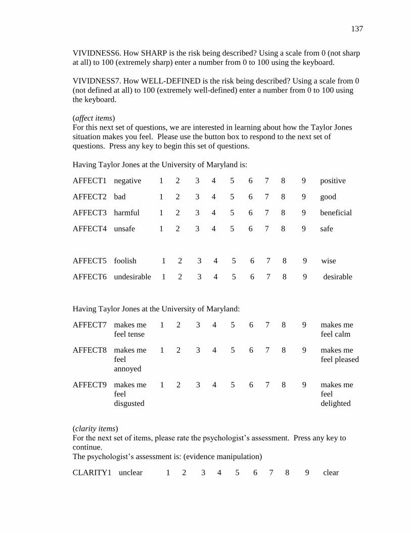
137

VIVIDNESS6. How SHARP is the risk being described? Using a scale from 0 (not sharp

at all) to 100 (extremely sharp) enter a number from 0 to 100 using the keyboard.

VIVIDNESS7. How WELL-DEFINED is the risk being described? Using a scale from 0

(not defined at all) to 100 (extremely well-defined) enter a number from 0 to 100 using

the keyboard.

(affect items)

For this next set of questions, we are interested in learning about how the Taylor Jones

situation makes you feel. Please use the button box to respond to the next set of

questions. Press any key to begin this set of questions.

Having Taylor Jones at the University of Maryland is:

AFFECT1 negative 1 2 3 4 5 6 7 8 9 positive

AFFECT2 bad 1 2 3 4 5 6 7 8 9 good

AFFECT3 harmful 1 2 3 4 5 6 7 8 9 beneficial

AFFECT4 unsafe 1 2 3 4 5 6 7 8 9 safe

AFFECT5 foolish 1 2 3 4 5 6 7 8 9 wise

AFFECT6 undesirable 1 2 3 4 5 6 7 8 9 desirable

Having Taylor Jones at the University of Maryland:

AFFECT7 makes me

feel tense

1 2 3 4 5 6 7 8 9 makes me

feel calm

AFFECT8 makes me

feel

annoyed

1 2 3 4 5 6 7 8 9 makes me

feel pleased

AFFECT9 makes me

feel

disgusted

1 2 3 4 5 6 7 8 9 makes me

feel

delighted

(clarity items)

For the next set of items, please rate the psychologist‘s assessment. Press any key to

continue.

The psychologist‘s assessment is: (evidence manipulation)

CLARITY1 unclear 1 2 3 4 5 6 7 8 9 clear

138

CLARITY2 confusing 1 2 3 4 5 6 7 8 9 not

confusing

CLARITY3 hard to

understand

1 2 3 4 5 6 7 8 9 easy to

understand

CLARITY4 vague 1 2 3 4 5 6 7 8 9 precise

CLARITY5 not a

noticeable

point

1 2 3 4 5 6 7 8 9 a noticeable

point

CLARITY6 weak 1 2 3 4 5 6 7 8 9 strong

CLARITY7 abstract 1 2 3 4 5 6 7 8 9 concrete

CLARITY8 not relevant

to the

conclusion

1 2 3 4 5 6 7 8 9 relevant to

the

conclusion

(risk perception items)

This next set of questions will ask you how you feel about the Taylor Jones situation.

Use the keyboard to type your answers. Press any key when you are ready to begin.

(perceived susceptibility)

Using a scale from 0 (impossible to happen) to 100 (certain to happen):

SUS1. How certain are you that Taylor Jones will commit another act of violence?

SUS2. What is the chance that Taylor Jones will commit another act of violence?

SUS3. How likely is Taylor Jones to commit another act of violence?

(perceived severity)

Using a scale from 0 (no risk) to 100 (high risk):

SEV1. What is the risk of Taylor Jones committing another violent act?

SEV2. How dangerous is Taylor Jones?

SEV3. How serious is Taylor Jones‘s violent behavior?

(objective numeracy items)

For this next set of questions, read each question and use the keyboard to provide an

answer. Use the scratch paper next to your computer if you need it. Press any key to

begin.


disease? 1 in 100, 1 in 1,000, or 1 in 10? Please type your answer using the keyboard.

(Answer: 1 in 10)

ONUM2. Which of the following represents the biggest risk of getting a disease: 1%,

10%, or 5%? Please type you answer using the keyboard. (Answer: 10%)

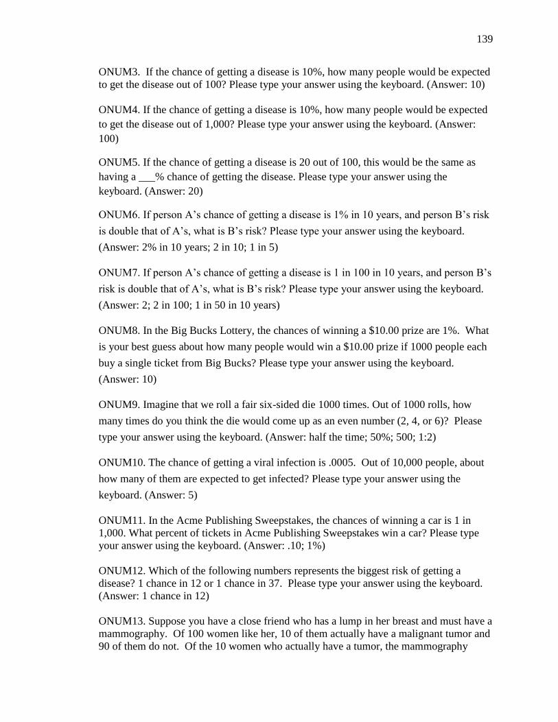
139


to get the disease out of 100? Please type your answer using the keyboard. (Answer: 10)


to get the disease out of 1,000? Please type your answer using the keyboard. (Answer:

100)

ONUM5. If the chance of getting a disease is 20 out of 100, this would be the same as

having a ___% chance of getting the disease. Please type your answer using the


ONUM6. If person A‘s chance of getting a disease is 1% in 10 years, and person B‘s risk

is double that of A‘s, what is B‘s risk? Please type your answer using the keyboard.

(Answer: 2% in 10 years; 2 in 10; 1 in 5)

ONUM7. If person A‘s chance of getting a disease is 1 in 100 in 10 years, and person B‘s

risk is double that of A‘s, what is B‘s risk? Please type your answer using the keyboard.

(Answer: 2; 2 in 100; 1 in 50 in 10 years)

ONUM8. In the Big Bucks Lottery, the chances of winning a $10.00 prize are 1%. What

is your best guess about how many people would win a $10.00 prize if 1000 people each

buy a single ticket from Big Bucks? Please type your answer using the keyboard.

(Answer: 10)

ONUM9. Imagine that we roll a fair six-sided die 1000 times. Out of 1000 rolls, how

many times do you think the die would come up as an even number (2, 4, or 6)? Please

type your answer using the keyboard. (Answer: half the time; 50%; 500; 1:2)

ONUM10. The chance of getting a viral infection is .0005. Out of 10,000 people, about

how many of them are expected to get infected? Please type your answer using the


ONUM11. In the Acme Publishing Sweepstakes, the chances of winning a car is 1 in

1,000. What percent of tickets in Acme Publishing Sweepstakes win a car? Please type

your answer using the keyboard. (Answer: .10; 1%)


disease? 1 chance in 12 or 1 chance in 37. Please type your answer using the keyboard.

(Answer: 1 chance in 12)

ONUM13. Suppose you have a close friend who has a lump in her breast and must have a

mammography. Of 100 women like her, 10 of them actually have a malignant tumor and

90 of them do not. Of the 10 women who actually have a tumor, the mammography

140

indicates correctly that 9 of them have a tumor and indicates incorrectly that 1 of them

does not have a tumor. Of the 90 women who do not have a tumor, the mammography

indicates correctly that 81 of them do not have a tumor and indicates incorrectly that 9 of

them do have a tumor. Imagine that your friend test positive (as if she had a tumor).

What is the likelihood that she actually has a tumor? Please type your answer using the

keyboard. (Answer: 9 out of 18; 1 out of 2; 50%; 1:2)

ONUM14. Imagine that you are taking a class and your chances of being asked a

question in class are 1% during the first week of class and double each week thereafter

(i.e., you would have a 2% chance in Week 2, a 4% chance in week 3, and 8% chance in

week 4). What is the probability that you will be asked a question in class during week

7? Please type your answer using the keyboard. (Answer: 64%)

ONUM15. Suppose that 1 out of every 10,000 doctors in a certain regimen is infected

with the SARS virus; in the same region, 20 out of every 100 people in a particular at-risk

population are also infected with the virus. A test for the virus gives a positive result in

99% of those who are infected and in 1% of those who are not infected. A randomly

selected doctor and a randomly selected person in the at-risk population in this region

both test positive for the disease. Who is more likely to actually have the disease? Enter

A, B, or C using the keyboard. (Answer: C)

A. They both tested positive for SARS and therefore are equally likely to have the disease

B. They both tested positive for SARS and the doctor is more likely to have the disease

C. They both tested positive for SARS and the person in the at-risk population is more

likely to have the disease

(subjective numeracy items)

For this next set of questions, please choose one response using the 1 - 9 scale on the

button box. Press any key to begin.

SNUM1. How good are you at working with fractions? (1 = not good at all, 9 =

extremely good)

SNUM2. How good are you at working with percentages? (1 = not good at all, 9 =

extremely good)

SNUM3. How good are you at calculating a 15% tip on a bill? (1 = not good at all, 9 =

extremely good)

SNUM4. How good are you at figuring out how much a shirt will cost if it is marked

25% off? (1 = not good at all, 9 = extremely good)

SNUM5. When reading the newspaper, how helpful do you find tables and graphs that

are part of a story? (1 = not helpful at all, 9 = extremely helpful)

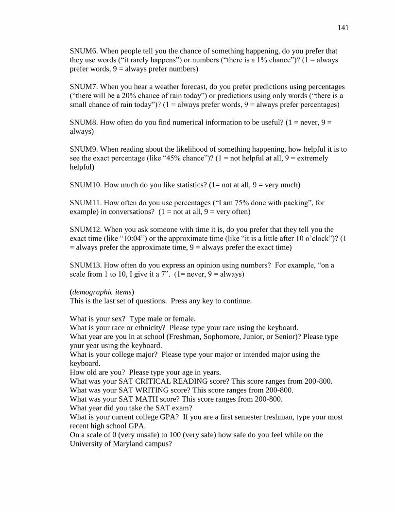
141

SNUM6. When people tell you the chance of something happening, do you prefer that

they use words (―it rarely happens‖) or numbers (―there is a 1% chance‖)? (1 = always

prefer words, 9 = always prefer numbers)

SNUM7. When you hear a weather forecast, do you prefer predictions using percentages

(―there will be a 20% chance of rain today‖) or predictions using only words (―there is a

small chance of rain today‖)? (1 = always prefer words, 9 = always prefer percentages)

SNUM8. How often do you find numerical information to be useful? (1 = never, 9 =

always)

SNUM9. When reading about the likelihood of something happening, how helpful it is to

see the exact percentage (like ―45% chance‖)? (1 = not helpful at all, 9 = extremely

helpful)

SNUM10. How much do you like statistics? (1= not at all, 9 = very much)

SNUM11. How often do you use percentages (―I am 75% done with packing‖, for

example) in conversations? (1 = not at all, 9 = very often)

SNUM12. When you ask someone with time it is, do you prefer that they tell you the

exact time (like ―10:04‖) or the approximate time (like ―it is a little after 10 o‘clock‖)? (1

= always prefer the approximate time, 9 = always prefer the exact time)

SNUM13. How often do you express an opinion using numbers? For example, ―on a

scale from 1 to 10, I give it a 7‖. (1= never, 9 = always)

(demographic items)

This is the last set of questions. Press any key to continue.

What is your sex? Type male or female.

What is your race or ethnicity? Please type your race using the keyboard.

What year are you in at school (Freshman, Sophomore, Junior, or Senior)? Please type

your year using the keyboard.

What is your college major? Please type your major or intended major using the

keyboard.

How old are you? Please type your age in years.

What was your SAT CRITICAL READING score? This score ranges from 200-800.

What was your SAT WRITING score? This score ranges from 200-800.

What was your SAT MATH score? This score ranges from 200-800.

What year did you take the SAT exam?

What is your current college GPA? If you are a first semester freshman, type your most

recent high school GPA.

On a scale of 0 (very unsafe) to 100 (very safe) how safe do you feel while on the

University of Maryland campus?

142

Do you have any questions or comments about this survey? Please let us know if any

questions were unclear or if you could not read any question that appeared on your

screen.

Please STOP here! Thank you. We appreciate your participation in this research study!

Let the researcher know that you are finished. This project is ongoing. Please do not

share the details of this research project with anyone else. If you have any questions feel

free to contact the researcher, Christine Skubisz at [email protected]. The information

you read in this study is fictitious and does not refer to any previous or current UMD

students. Leave your papers at your computer station.

143

Appendix D

Covariance Matrix for the Evolutionary Model (Study 1)

FORM1 FORM2 FORM3 ONUM FORMxONUM

FORM1 0.19

FORM2 - 0.07 0.19

FORM3 - 0.06 - 0.07 0.19

ONUM 0.00 - 0.02 0.00 4.59

FORMxONUM 0.01 - 0.07 0.02 11.42 33.93

SNUM - 0.02 0.07 - 0.04 - 1.47 - 3.85

RT - 0.00 0.01 0.00 - 0.04 - 0.10

CLARITY1 0.04 0.04 0.00 0.07 0.01

CLARITY2 0.08 0.02 0.02 - 0.18 - 0.47

CLARITY4 0.02 0.01 - 0.02 0.02 - 0.09

SUS1 0.40 0.89 - 0.75 2.92 9.07

SUS2 0.79 1.15 - 0.97 2.90 9.28

SUS3 0.95 1.13 - 0.89 2.67 9.52

SEV1 1.01 1.00 - 1.58 5.03 16.54

SEV2 0.77 0.33 - 1.03 6.86 23.66

DEC 0.31 0.42 - 0.86 8.28 22.46

SNUM RT CLARITY1 CLARITY2 CLARITY4

SNUM 2.07

RT 0.02 0.03

CLARITY1 0.01 - 0.01 7.16

CLARITY2 0.20 0.02 4.55 6.63

CLARITY4 0.10 - 0.02 4.93 3.71 6.81

SUS1 1.49 0.79 - 22.78 - 16.34 - 24.11

SUS2 0.95 0.68 -23.26 -16.58 - 23.45

SUS3 1.52 0.62 -23.77 - 15.72 - 25.13

SEV1 - 1.32 0.52 -17.27 - 14.80 - 21.50

SEV2 - 1.25 0.24 -7.56 - 6.12 - 7.75

DEC - 3.18 0.37 -21.44 -15.76 -21.61

SUS1 SUS2 SUS3 SEV1 SEV2 DEC

SUS1 1475.90

SUS2 1367.19 1506.15

SUS3 1317.06 1420.09 1462.97

SEV1 1074.92 1178.89 1176.07 1361.92

SEV2 716.67 768.75 767.16 803.54 997.61

DEC 818.29 862.15 870.44 793.41 604.97 1298.30

144

Appendix E

Covariance Matrix for the Affective Processing Model (Study 1)


FORM1 0.19

FORM2 - 0.07 0.19

FORM3 - 0.06 - 0.07 0.19

ONUM 0.00 - 0.02 0.00 4.59

FORMxONUM 0.01 - 0.07 0.02 11.42 33.93

SNUM - 0.02 0.07 - 0.04 - 1.47 - 3.85

RT - 0.00 0.01 0.00 - 0.04 - 0.10

AFFECT1 - 0.05 0.00 0.04 0.32 0.88

AFFECT6 0.03 - 0.08 0.07 0.32 1.32

VIVIDNESS1 0.25 1.02 - 0.39 6.14 13.23

VIVIDNESS2 - 0.41 - 0.31 0.68 6.32 14.78

VIVIDNESS3 - 0.20 0.02 1.33 2.51 5.62

SUS1 0.40 0.89 - 0.75 2.92 9.07

SUS2 0.79 1.15 - 0.97 2.90 9.28

SUS3 0.95 1.13 - 0.89 2.67 9.52

SEV1 1.01 1.00 - 1.58 5.03 16.54

SEV2 0.77 0.33 - 1.03 6.86 23.66

DEC 0.31 0.42 - 0.86 8.28 22.46


SNUM 2.07

RT 0.02 0.03

AFFECT1 - 0.03 - 0.03 1.17 0.90 1.03

AFFECT6 - 0.29 - 0.03 0.98 0.87 1.07

VIVIDNESS1 2.43 - 0.24 40.51 36.80 34.74

VIVIDNESS2 - 3.85 - 0.10 39.99 26.77 38.74

VIVIDNESS3 - 1.67 0.18 26.93 16.77 25.15

SUS1 1.49 0.79 - 22.78 - 16.34 - 24.11

SUS2 0.95 0.68 -23.26 -16.58 - 23.45

SUS3 1.52 0.62 -23.77 - 15.72 - 25.13

SEV1 - 1.32 0.52 -17.27 - 14.80 - 21.50

SEV2 - 1.25 0.24 -7.56 - 6.12 - 7.75

DEC - 3.18 0.37 -21.44 -15.76 -21.61

AFFECT1 AFFECT6 VIVIDNESS1 VIVIDNESS2 VIVIDNESS3

AFFECT1 2.77

AFFECT6 1.48 3.54

VIVIDNESS1 12.10 10.23 1235.88

VIVIDNESS2 10.38 11.17 326.65 865.44

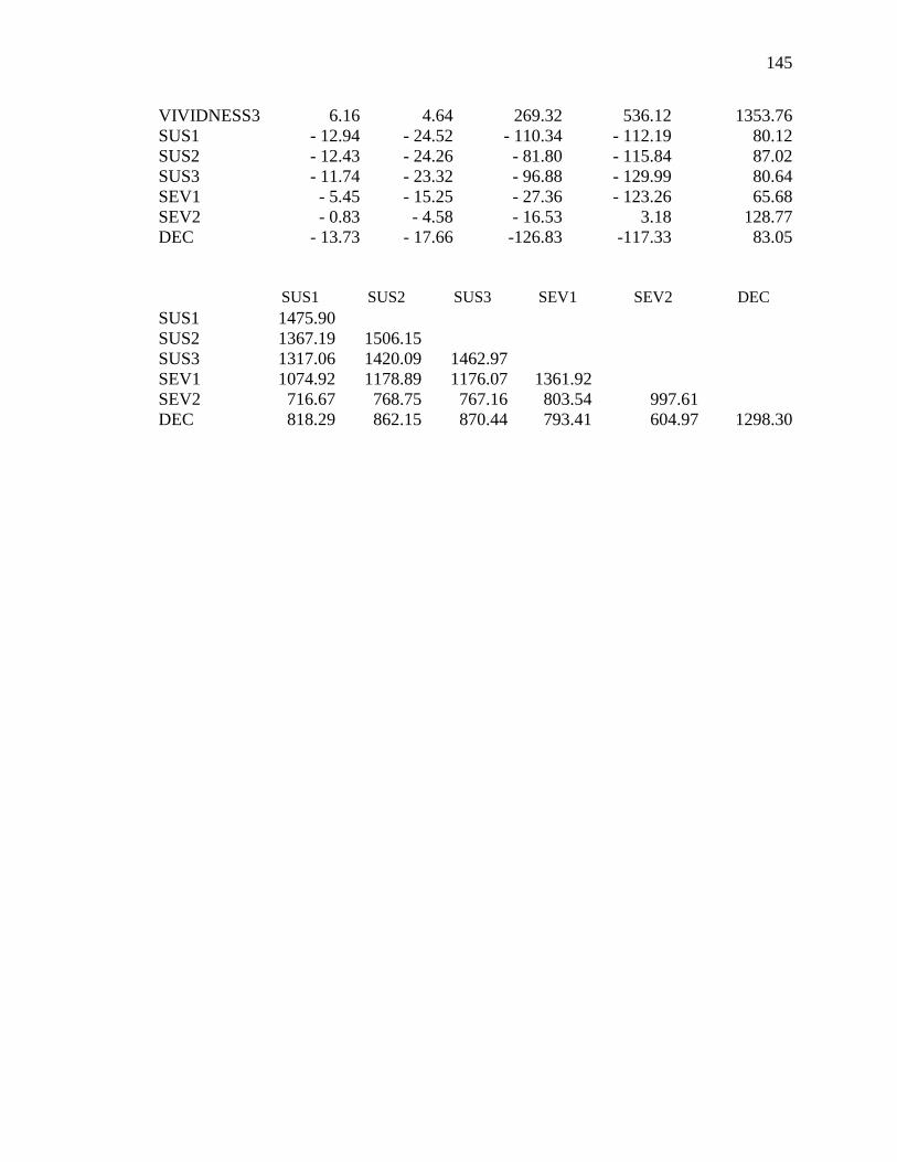
145

VIVIDNESS3 6.16 4.64 269.32 536.12 1353.76

SUS1 - 12.94 - 24.52 - 110.34 - 112.19 80.12

SUS2 - 12.43 - 24.26 - 81.80 - 115.84 87.02

SUS3 - 11.74 - 23.32 - 96.88 - 129.99 80.64

SEV1 - 5.45 - 15.25 - 27.36 - 123.26 65.68

SEV2 - 0.83 - 4.58 - 16.53 3.18 128.77

DEC - 13.73 - 17.66 -126.83 -117.33 83.05


SUS1 1475.90

SUS2 1367.19 1506.15

SUS3 1317.06 1420.09 1462.97

SEV1 1074.92 1178.89 1176.07 1361.92

SEV2 716.67 768.75 767.16 803.54 997.61

DEC 818.29 862.15 870.44 793.41 604.97 1298.30

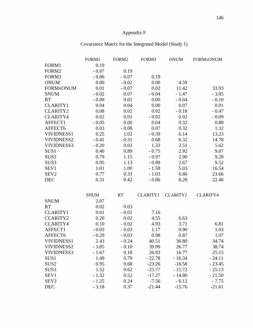
146

Appendix F

Covariance Matrix for the Integrated Model (Study 1)


FORM1 0.19

FORM2 - 0.07 0.19

FORM3 - 0.06 - 0.07 0.19

ONUM 0.00 - 0.02 0.00 4.59

FORMxONUM 0.01 - 0.07 0.02 11.42 33.93

SNUM - 0.02 0.07 - 0.04 - 1.47 - 3.85

RT - 0.00 0.01 0.00 - 0.04 - 0.10

CLARITY1 0.04 0.04 0.00 0.07 0.01

CLARITY2 0.08 0.02 0.02 - 0.18 - 0.47

CLARITY4 0.02 0.01 - 0.02 0.02 - 0.09

AFFECT1 - 0.05 0.00 0.04 0.32 0.88

AFFECT6 0.03 - 0.08 0.07 0.32 1.32

VIVIDNESS1 0.25 1.02 - 0.39 6.14 13.23

VIVIDNESS2 - 0.41 - 0.31 0.68 6.32 14.78

VIVIDNESS3 - 0.20 0.02 1.33 2.51 5.62

SUS1 0.40 0.89 - 0.75 2.92 9.07

SUS2 0.79 1.15 - 0.97 2.90 9.28

SUS3 0.95 1.13 - 0.89 2.67 9.52

SEV1 1.01 1.00 - 1.58 5.03 16.54

SEV2 0.77 0.33 - 1.03 6.86 23.66

DEC 0.31 0.42 - 0.86 8.28 22.46


SNUM 2.07

RT 0.02 0.03

CLARITY1 0.01 - 0.01 7.16

CLARITY2 0.20 0.02 4.55 6.63

CLARITY4 0.10 - 0.02 4.93 3.71 6.81

AFFECT1 - 0.03 - 0.03 1.17 0.90 1.03

AFFECT6 - 0.29 - 0.03 0.98 0.87 1.07

VIVIDNESS1 2.43 - 0.24 40.51 36.80 34.74

VIVIDNESS2 - 3.85 - 0.10 39.99 26.77 38.74

VIVIDNESS3 - 1.67 0.18 26.93 16.77 25.15

SUS1 1.49 0.79 - 22.78 - 16.34 - 24.11

SUS2 0.95 0.68 -23.26 -16.58 - 23.45

SUS3 1.52 0.62 -23.77 - 15.72 - 25.13

SEV1 - 1.32 0.52 -17.27 - 14.80 - 21.50

SEV2 - 1.25 0.24 -7.56 - 6.12 - 7.75

DEC - 3.18 0.37 -21.44 -15.76 -21.61

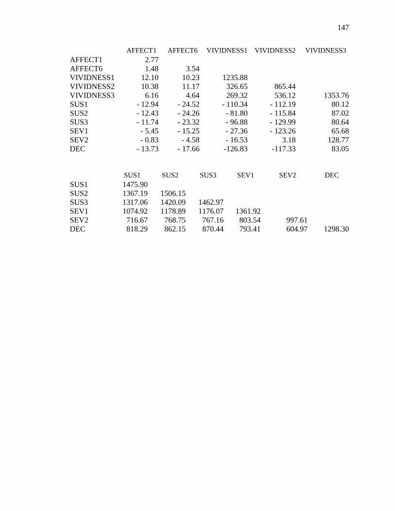
147

AFFECT1 AFFECT6 VIVIDNESS1 VIVIDNESS2 VIVIDNESS3

AFFECT1 2.77

AFFECT6 1.48 3.54

VIVIDNESS1 12.10 10.23 1235.88

VIVIDNESS2 10.38 11.17 326.65 865.44

VIVIDNESS3 6.16 4.64 269.32 536.12 1353.76

SUS1 - 12.94 - 24.52 - 110.34 - 112.19 80.12

SUS2 - 12.43 - 24.26 - 81.80 - 115.84 87.02

SUS3 - 11.74 - 23.32 - 96.88 - 129.99 80.64

SEV1 - 5.45 - 15.25 - 27.36 - 123.26 65.68

SEV2 - 0.83 - 4.58 - 16.53 3.18 128.77

DEC - 13.73 - 17.66 -126.83 -117.33 83.05


SUS1 1475.90

SUS2 1367.19 1506.15

SUS3 1317.06 1420.09 1462.97

SEV1 1074.92 1178.89 1176.07 1361.92

SEV2 716.67 768.75 767.16 803.54 997.61

DEC 818.29 862.15 870.44 793.41 604.97 1298.30

148

Appendix G

Covariance Matrix for the Evolutionary Model (Study 2)


FORM1 0.18

FORM2 -0.05 0.17

FORM3 -0.06 -0.06 0.20

ONUM 0.02 -0.01 -0.01 5.10

FORMxONUM 0.03 -0.01 -0.02 13.62 41.98

SNUM -0.02 -0.03 0.03 1.34 3.38

RT 0.00 0.00 0.00 0.05 0.13

CLARITY1 -0.06 0.08 0.01 0.07 -0.08

CLARITY2 -0.02 0.12 0.06 0.76 2.03

CLARITY3 -0.04 0.15 0.08 0.51 1.19

CLARITY4 -0.05 0.07 0.03 0.20 0.46

CLARITY5 0.03 0.02 0.04 0.50 1.07

CLARITY6 -0.02 0.01 0.03 0.17 0.38

CLARITY7 -0.11 0.07 0.04 0.10 0.20

CLARITY8 0.05 0.01 -0.02 0.58 1.18

SUS1 0.75 -0.29 -0.27 -3.99 -11.73

SUS2 0.51 -0.01 -0.64 -7.71 -19.93

SUS3 -0.09 0.03 0.10 -8.16 -20.96

SEV1 0.22 0.49 -0.29 -4.77 -14.08

SEV2 0.13 0.15 0.43 -1.03 -3.62

DEC1 0.04 0.09 -0.11 -0.07 -0.26

DEC2 0.03 0.08 -0.09 0.43 0.93

DEC3 0.05 0.07 -0.10 0.53 1.13

DEC5 0.01 0.10 -0.05 0.39 0.82


SNUM 2.04

RT 0.01 0.03

CLARITY1 0.39 -0.01 4.95

CLARITY2 0.35 0.01 3.34 6.36

CLARITY3 0.42 0.02 2.94 4.89 6.21

CLARITY4 0.25 0.00 3.34 2.65 2.62

CLARITY5 0.59 0.02 2.44 2.64 2.93

CLARITY6 0.28 0.00 2.94 2.60 2.44

CLARITY7 0.09 0.02 2.39 2.52 2.46

CLARITY8 0.38 0.03 1.93 2.51 2.22

SUS1 -3.76 -0.26 -4.58 -7.84 -9.03

SUS2 -5.43 -0.26 -5.72 -8.62 -7.03

SUS3 -5.17 -0.17 -5.13 -9.88 -8.83

SEV1 -2.73 0.17 -7.04 -9.05 -5.59

SEV2 -1.10 -0.13 -0.34 -2.62 -3.73

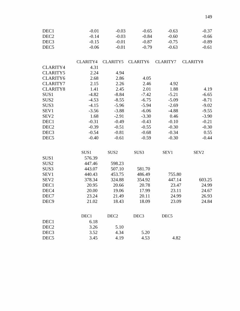
149

DEC1 -0.01 -0.03 -0.65 -0.63 -0.37

DEC2 -0.14 -0.03 -0.84 -0.60 -0.66

DEC3 -0.15 -0.01 -0.87 -0.75 -0.89

DEC5 -0.06 -0.01 -0.79 -0.63 -0.61

CLARITY4 CLARITY5 CLARITY6 CLARITY7 CLARITY8

CLARITY4 4.31

CLARITY5 2.24 4.94

CLARITY6 2.68 2.86 4.05

CLARITY7 2.15 2.26 2.46 4.92

CLARITY8 1.41 2.45 2.01 1.88 4.19

SUS1 -4.82 -8.84 -7.42 -5.21 -6.65

SUS2 -4.53 -8.55 -6.75 -5.09 -8.71

SUS3 -4.15 -5.96 -5.94 -2.69 -9.02

SEV1 -3.56 -3.88 -6.06 -4.88 -9.55

SEV2 1.68 -2.91 -3.30 0.46 -3.90

DEC1 -0.31 -0.49 -0.43 -0.10 -0.21

DEC2 -0.39 -0.51 -0.55 -0.30 -0.30

DEC3 -0.54 -0.81 -0.68 -0.34 0.55

DEC5 -0.40 -0.61 -0.59 -0.30 -0.44

SUS1 SUS2 SUS3 SEV1 SEV2

SUS1 576.39

SUS2 447.46 598.23

SUS3 443.07 507.10 581.70

SEV1 440.43 453.75 486.49 755.80

SEV2 378.34 324.88 354.92 447.14 603.25

DEC1 20.95 20.66 20.78 23.47 24.99

DEC4 20.00 19.06 17.99 23.11 24.67

DEC7 23.24 21.49 20.11 24.99 26.93

DEC9 21.02 18.43 18.09 23.09 24.84

DEC1 DEC2 DEC3 DEC5

DEC1 6.18

DEC2 3.26 5.10

DEC3 3.52 4.34 5.20

DEC5 3.45 4.19 4.53 4.82

150

Appendix H

Covariance Matrix for the Affective Processing Model (Study 2)


FORM1 0.18

FORM2 -0.05 0.17

FORM3 -0.06 -0.06 0.20

ONUM 0.02 -0.01 -0.01 5.10

FORMxONUM 0.03 -0.01 -0.02 13.62 41.98

SNUM -0.02 -0.03 0.03 1.34 3.38

RT 0.00 0.00 0.00 0.05 0.13

AFFECT1 -0.03 -0.04 0.03 -0.28 -0.77

AFFECT2 -0.02 -0.01 0.01 -0.35 -0.89

AFFECT3 0.01 -0.02 -0.01 -0.20 -0.58

AFFECT4 -0.02 -0.06 0.03 -0.36 -0.92

AFFECT5 -0.03 -0.03 0.02 -0.28 -0.59

AFFECT6 0.00 -0.04 0.03 -0.19 -0.27

AFFECT7 -0.04 -0.07 0.05 -0.24 -0.56

AFFECT8 -0.02 -0.01 0.01 -0.16 -0.21

AFFECT9 -0.01 -0.03 0.02 0.04 0.26

VIVIDNESS1 -0.40 0.88 0.37 0.56 -1.92

VIVIDNESS2 -0.56 0.54 0.35 -1.96 -5.38

VIVIDNESS3 -1.11 0.31 0.49 -1.20 -3.32

VIVIDNESS4 0.39 -0.64 0.02 -3.41 -14.24

VIVIDNESS5 -0.43 1.19 -0.11 -6.90 -26.30

VIVIDNESS6 -0.21 0.49 0.27 -4.74 -20.91

VIVIDNESS7 -1.47 0.30 1.24 3.59 5.79

SUS1 0.75 -0.29 -0.27 -3.99 -11.73

SUS2 0.51 -0.01 -0.64 -7.71 -19.93

SUS3 -0.09 0.03 0.10 -8.16 -20.96

SEV1 0.22 0.49 -0.29 -4.77 -14.08

SEV2 0.13 0.15 0.43 -1.03 -3.62

DEC1 0.04 0.09 -0.11 -0.07 -0.26

DEC2 0.03 0.08 -0.09 0.43 0.93

DEC3 0.05 0.07 -0.10 0.53 1.13

DEC5 0.01 0.10 -0.05 0.39 0.82

AFFECT1 AFFECT2 AFFECT3 AFFECT4 AFFECT5

AFFECT1 3.06

AFFECT2 2.48 2.61

AFFECT3 2.08 2.01 2.38

AFFECT4 2.17 2.07 1.98 2.52

AFFECT5 2.17 2.18 1.89 2.02 2.72

AFFECT6 2.25 2.17 1.89 1.94 2.20

AFFECT7 1.81 1.79 1.66 1.86 1.73

151

AFFECT8 2.04 1.88 1.61 1.69 1.97

AFFECT9 1.48 1.79 1.26 1.30 1.51

VIVIDNESS1 4.41 5.03 2.83 2.99 4.16

VIVIDNESS2 3.81 2.46 1.88 1.36 2.64

VIVIDNESS3 5.16 3.73 3.24 2.58 5.00

VIVIDNESS4 -2.82 -0.79 -2.12 -3.72 -0.77

VIVIDNESS5 6.08 5.72 0.98 2.71 5.42

VIVIDNESS6 6.71 5.89 2.39 4.16 5.59

VIVIDNESS7 4.72 2.81 0.63 1.29 4.32

SUS1 -15.05 -15.42 -14.15 -16.14 -15.41

SUS2 -12.78 -12.86 -12.89 -13.40 -14.23

SUS3 -12.65 -13.35 -12.89 -13.98 -12.94

SEV1 -17.32 -17.76 -17.11 -19.20 -17.10

SEV2 -18.86 -19.98 -18.64 -21.31 -19.06

DEC1 -2.44 -2.29 -2.05 -2.17 -2.41

DEC2 -2.74 -2.48 -2.17 -2.47 -2.65

DEC3 -2.77 -2.67 -2.24 -2.52 -2.84

DEC5 -2.74 -2.62 -2.24 -2.51 -2.76

AFFECT6 AFFECT7 AFFECT8 AFFECT9 VIVIDNESS1

AFFECT6 2.83

AFFECT7 1.80 2.77

AFFECT8 1.96 1.76 2.74

AFFECT9 1.50 1.27 1.69 1.69

VIVIDNESS1 1.38 2.43 4.07 0.67 905.12

VIVIDNESS2 1.72 3.33 3.24 1.25 293.87

VIVIDNESS3 3.77 2.12 2.96 -0.07 370.33

VIVIDNESS4 -2.22 -1.42 -1.45 -1.36 167.59

VIVIDNESS5 4.70 0.67 5.44 3.31 187.35

VIVIDNESS6 5.03 3.39 5.41 2.38 256.42

VIVIDNESS7 1.03 0.38 4.02 1.80 360.44

SUS1 -13.26 -14.41 -12.76 -10.91 -43.85

SUS2 -11.79 -12.77 -11.07 -9.36 -53.79

SUS3 -11.38 -12.99 -10.62 -9.77 -44.22

SEV1 -17.09 -17.12 -14.29 -12.44 -41.06

SEV2 -18.98 -17.59 -15.28 -13.39 -21.86

DEC1 -2.21 -1.88 -2.07 -1.73 -4.12

DEC2 -2.50 -2.18 -2.29 -1.76 -2.72

DEC3 -2.69 -2.24 -2.39 -1.82 -3.04

DEC5 -2.69 -2.17 -2.39 -1.86 -2.01

VIVIDNESS2 VIVIDNESS3 VIVIDNESS4 VIVIDNESS5 VIVIDNESS6

VIVIDNESS2 625.23

VIVIDNESS3 385.78 787.60

VIVIDNESS4 231.47 404.05 815.24

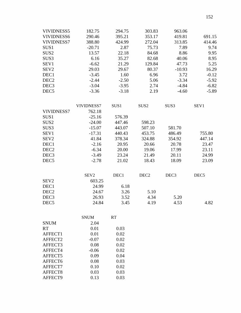
152

VIVIDNESS5 182.75 294.75 303.83 963.06

VIVIDNESS6 290.46 395.21 353.17 419.81 691.15

VIVIDNESS7 388.80 424.99 272.04 313.85 414.46

SUS1 -20.71 2.87 75.73 7.89 9.74

SUS2 13.57 22.18 84.68 8.86 9.95

SUS3 6.16 35.27 82.68 40.06 8.95

SEV1 -6.62 21.29 129.84 47.73 5.25

SEV2 29.03 29.67 80.37 -10.93 16.29

DEC1 -3.45 1.60 6.96 3.72 -0.12

DEC2 -2.44 -2.50 5.06 -3.34 -5.92

DEC3 -3.04 -3.95 2.74 -4.84 -6.82

DEC5 -3.36 -3.18 2.19 -4.60 -5.89

VIVIDNESS7 SUS1 SUS2 SUS3 SEV1

VIVIDNESS7 762.18

SUS1 -25.16 576.39

SUS2 -24.00 447.46 598.23

SUS3 -15.07 443.07 507.10 581.70

SEV1 -17.31 440.43 453.75 486.49 755.80

SEV2 41.84 378.34 324.88 354.92 447.14

DEC1 -2.16 20.95 20.66 20.78 23.47

DEC2 -6.34 20.00 19.06 17.99 23.11

DEC3 -3.49 23.24 21.49 20.11 24.99

DEC5 -2.78 21.02 18.43 18.09 23.09

SEV2 DEC1 DEC2 DEC3 DEC5

SEV2 603.25

DEC1 24.99 6.18

DEC2 24.67 3.26 5.10

DEC3 26.93 3.52 4.34 5.20

DEC5 24.84 3.45 4.19 4.53 4.82

SNUM RT

SNUM 2.04

RT 0.01 0.03

AFFECT1 0.01 0.02

AFFECT2 -0.07 0.02

AFFECT3 0.08 0.02

AFFECT4 -0.06 0.02

AFFECT5 0.09 0.04

AFFECT6 0.08 0.03

AFFECT7 0.10 0.02

AFFECT8 0.03 0.03

AFFECT9 0.13 0.03

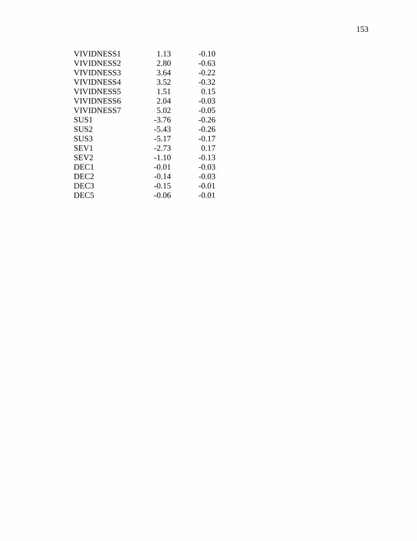
153

VIVIDNESS1 1.13 -0.10




VIVIDNESS5 1.51 0.15



SUS1 -3.76 -0.26

SUS2 -5.43 -0.26

SUS3 -5.17 -0.17

SEV1 -2.73 0.17

SEV2 -1.10 -0.13

DEC1 -0.01 -0.03

DEC2 -0.14 -0.03

DEC3 -0.15 -0.01

DEC5 -0.06 -0.01

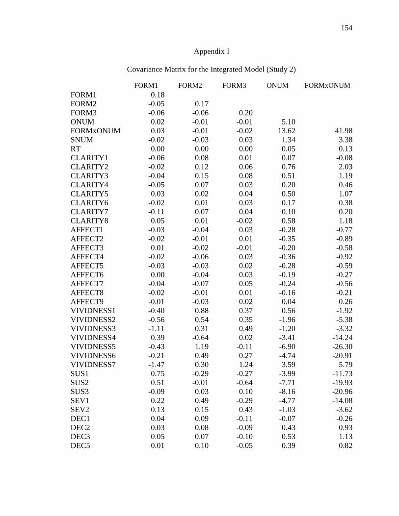
154

Appendix I

Covariance Matrix for the Integrated Model (Study 2)


FORM1 0.18

FORM2 -0.05 0.17

FORM3 -0.06 -0.06 0.20

ONUM 0.02 -0.01 -0.01 5.10

FORMxONUM 0.03 -0.01 -0.02 13.62 41.98

SNUM -0.02 -0.03 0.03 1.34 3.38

RT 0.00 0.00 0.00 0.05 0.13

CLARITY1 -0.06 0.08 0.01 0.07 -0.08

CLARITY2 -0.02 0.12 0.06 0.76 2.03

CLARITY3 -0.04 0.15 0.08 0.51 1.19

CLARITY4 -0.05 0.07 0.03 0.20 0.46

CLARITY5 0.03 0.02 0.04 0.50 1.07

CLARITY6 -0.02 0.01 0.03 0.17 0.38

CLARITY7 -0.11 0.07 0.04 0.10 0.20

CLARITY8 0.05 0.01 -0.02 0.58 1.18

AFFECT1 -0.03 -0.04 0.03 -0.28 -0.77

AFFECT2 -0.02 -0.01 0.01 -0.35 -0.89

AFFECT3 0.01 -0.02 -0.01 -0.20 -0.58

AFFECT4 -0.02 -0.06 0.03 -0.36 -0.92

AFFECT5 -0.03 -0.03 0.02 -0.28 -0.59

AFFECT6 0.00 -0.04 0.03 -0.19 -0.27

AFFECT7 -0.04 -0.07 0.05 -0.24 -0.56

AFFECT8 -0.02 -0.01 0.01 -0.16 -0.21

AFFECT9 -0.01 -0.03 0.02 0.04 0.26

VIVIDNESS1 -0.40 0.88 0.37 0.56 -1.92

VIVIDNESS2 -0.56 0.54 0.35 -1.96 -5.38

VIVIDNESS3 -1.11 0.31 0.49 -1.20 -3.32

VIVIDNESS4 0.39 -0.64 0.02 -3.41 -14.24

VIVIDNESS5 -0.43 1.19 -0.11 -6.90 -26.30

VIVIDNESS6 -0.21 0.49 0.27 -4.74 -20.91

VIVIDNESS7 -1.47 0.30 1.24 3.59 5.79

SUS1 0.75 -0.29 -0.27 -3.99 -11.73

SUS2 0.51 -0.01 -0.64 -7.71 -19.93

SUS3 -0.09 0.03 0.10 -8.16 -20.96

SEV1 0.22 0.49 -0.29 -4.77 -14.08

SEV2 0.13 0.15 0.43 -1.03 -3.62

DEC1 0.04 0.09 -0.11 -0.07 -0.26

DEC2 0.03 0.08 -0.09 0.43 0.93

DEC3 0.05 0.07 -0.10 0.53 1.13

DEC5 0.01 0.10 -0.05 0.39 0.82

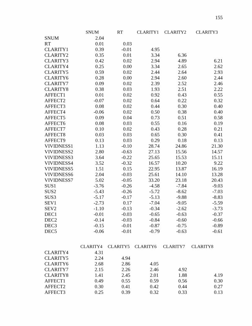
155


SNUM 2.04

RT 0.01 0.03

CLARITY1 0.39 -0.01 4.95

CLARITY2 0.35 0.01 3.34 6.36

CLARITY3 0.42 0.02 2.94 4.89 6.21

CLARITY4 0.25 0.00 3.34 2.65 2.62

CLARITY5 0.59 0.02 2.44 2.64 2.93

CLARITY6 0.28 0.00 2.94 2.60 2.44

CLARITY7 0.09 0.02 2.39 2.52 2.46

CLARITY8 0.38 0.03 1.93 2.51 2.22

AFFECT1 0.01 0.02 0.92 0.43 0.55

AFFECT2 -0.07 0.02 0.64 0.22 0.32

AFFECT3 0.08 0.02 0.44 0.30 0.40

AFFECT4 -0.06 0.02 0.50 0.38 0.40

AFFECT5 0.09 0.04 0.73 0.51 0.58

AFFECT6 0.08 0.03 0.55 0.16 0.19

AFFECT7 0.10 0.02 0.43 0.28 0.21

AFFECT8 0.03 0.03 0.65 0.30 0.41

AFFECT9 0.13 0.03 0.29 0.18 0.13

VIVIDNESS1 1.13 -0.10 28.74 24.86 21.30

VIVIDNESS2 2.80 -0.63 27.13 15.56 14.57

VIVIDNESS3 3.64 -0.22 25.65 15.53 15.11

VIVIDNESS4 3.52 -0.32 16.57 10.20 9.22

VIVIDNESS5 1.51 0.15 22.95 13.87 16.19

VIVIDNESS6 2.04 -0.03 25.61 14.10 13.28

VIVIDNESS7 5.02 -0.05 33.20 23.18 20.43

SUS1 -3.76 -0.26 -4.58 -7.84 -9.03

SUS2 -5.43 -0.26 -5.72 -8.62 -7.03

SUS3 -5.17 -0.17 -5.13 -9.88 -8.83

SEV1 -2.73 0.17 -7.04 -9.05 -5.59

SEV2 -1.10 -0.13 -0.34 -2.62 -3.73

DEC1 -0.01 -0.03 -0.65 -0.63 -0.37

DEC2 -0.14 -0.03 -0.84 -0.60 -0.66

DEC3 -0.15 -0.01 -0.87 -0.75 -0.89

DEC5 -0.06 -0.01 -0.79 -0.63 -0.61

CLARITY4 CLARITY5 CLARITY6 CLARITY7 CLARITY8

CLARITY4 4.31

CLARITY5 2.24 4.94

CLARITY6 2.68 2.86 4.05

CLARITY7 2.15 2.26 2.46 4.92

CLARITY8 1.41 2.45 2.01 1.88 4.19

AFFECT1 0.49 0.55 0.59 0.56 0.30

AFFECT2 0.30 0.41 0.42 0.44 0.27

AFFECT3 0.25 0.39 0.32 0.33 0.13

156

AFFECT4 0.18 0.39 0.44 0.30 0.26

AFFECT5 0.43 0.65 0.58 0.50 0.45

AFFECT6 0.37 0.35 0.35 0.41 0.14

AFFECT7 0.12 0.35 0.47 0.40 0.43

AFFECT8 0.36 0.52 0.58 0.65 0.53

AFFECT9 0.11 0.15 0.21 0.19 0.39

VIVIDNESS1 22.46 21.89 22.41 17.79 12.22

VIVIDNESS2 23.17 14.07 22.30 12.72 7.61

VIVIDNESS3 23.60 15.01 18.15 16.02 7.13

VIVIDNESS4 16.24 9.46 11.64 46.57 3.87

VIVIDNESS5 18.11 15.68 20.36 18.66 11.58

VIVIDNESS6 23.82 14.08 19.23 15.55 4.65

VIVIDNESS7 30.99 17.65 24.73 22.16 10.20

SUS1 -4.82 -8.84 -7.42 -5.21 -6.65

SUS2 -4.53 -8.55 -6.75 -5.09 -8.71

SUS3 -4.15 -5.96 -5.94 -2.69 -9.02

SEV1 -3.56 -3.88 -6.06 -4.88 -9.55

SEV2 1.68 -2.91 -3.30 0.46 -3.90

DEC1 -0.31 -0.49 -0.43 -0.10 -0.21

DEC2 -0.39 -0.51 -0.55 -0.30 -0.30

DEC3 -0.54 -0.81 -0.68 -0.34 0.55

DEC5 -0.40 -0.61 -0.59 -0.30 -0.44

AFFECT1 AFFECT2 AFFECT3 AFFECT4 AFFECT5

AFFECT1 3.06

AFFECT2 2.48 2.61

AFFECT3 2.08 2.01 2.38

AFFECT4 2.17 2.07 1.98 2.52

AFFECT5 2.17 2.18 1.89 2.02 2.72

AFFECT6 2.25 2.17 1.89 1.94 2.20

AFFECT7 1.81 1.79 1.66 1.86 1.73

AFFECT8 2.04 1.88 1.61 1.69 1.97

AFFECT9 1.48 1.79 1.26 1.30 1.51

VIVIDNESS1 4.41 5.03 2.83 2.99 4.16

VIVIDNESS2 3.81 2.46 1.88 1.36 2.64

VIVIDNESS3 5.16 3.73 3.24 2.58 5.00

VIVIDNESS4 -2.82 -0.79 -2.12 -3.72 -0.77

VIVIDNESS5 6.08 5.72 0.98 2.71 5.42

VIVIDNESS6 6.71 5.89 2.39 4.16 5.59

VIVIDNESS7 4.72 2.81 0.63 1.29 4.32

SUS1 -15.05 -15.42 -14.15 -16.14 -15.41

SUS2 -12.78 -12.86 -12.89 -13.40 -14.23

SUS3 -12.65 -13.35 -12.89 -13.98 -12.94

SEV1 -17.32 -17.76 -17.11 -19.20 -17.10

SEV2 -18.86 -19.98 -18.64 -21.31 -19.06

DEC1 -2.44 -2.29 -2.05 -2.17 -2.41

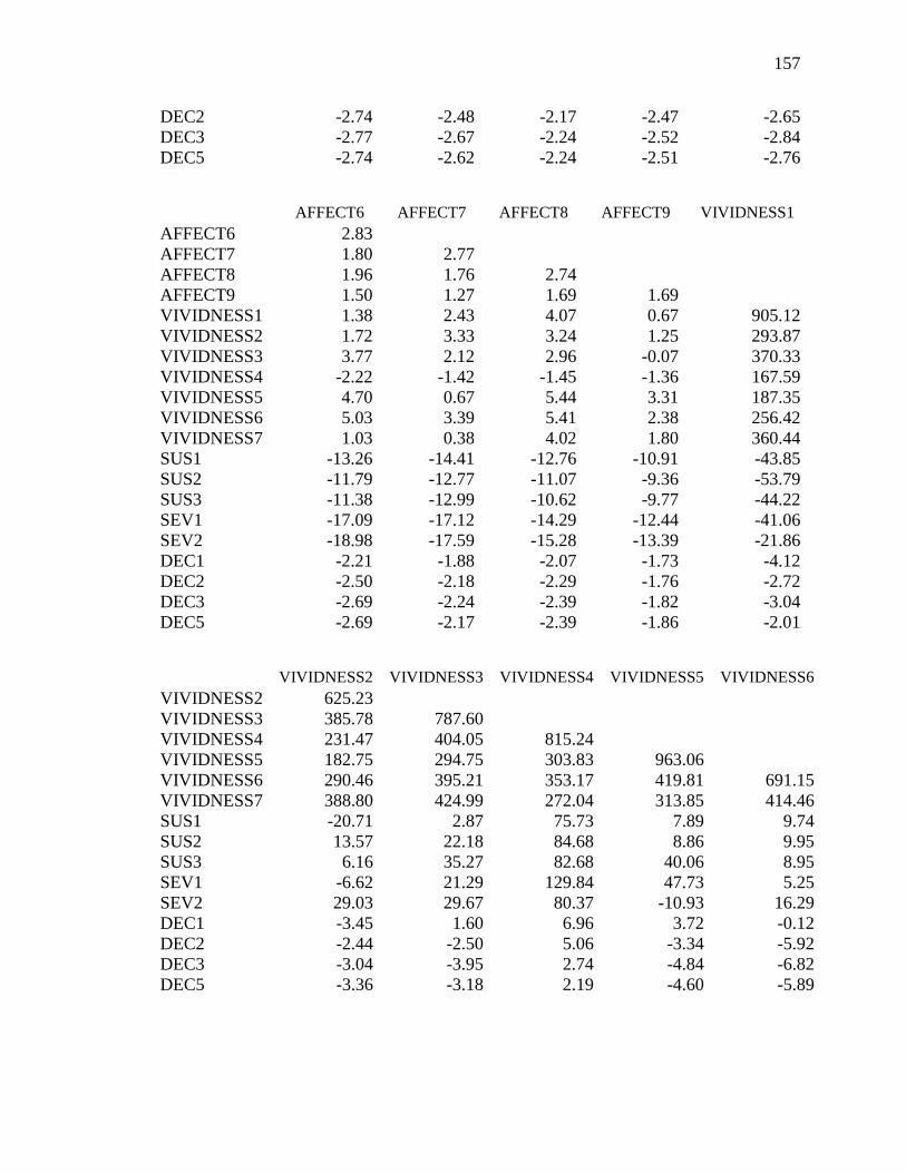
157

DEC2 -2.74 -2.48 -2.17 -2.47 -2.65

DEC3 -2.77 -2.67 -2.24 -2.52 -2.84

DEC5 -2.74 -2.62 -2.24 -2.51 -2.76

AFFECT6 AFFECT7 AFFECT8 AFFECT9 VIVIDNESS1

AFFECT6 2.83

AFFECT7 1.80 2.77

AFFECT8 1.96 1.76 2.74

AFFECT9 1.50 1.27 1.69 1.69

VIVIDNESS1 1.38 2.43 4.07 0.67 905.12

VIVIDNESS2 1.72 3.33 3.24 1.25 293.87

VIVIDNESS3 3.77 2.12 2.96 -0.07 370.33

VIVIDNESS4 -2.22 -1.42 -1.45 -1.36 167.59

VIVIDNESS5 4.70 0.67 5.44 3.31 187.35

VIVIDNESS6 5.03 3.39 5.41 2.38 256.42

VIVIDNESS7 1.03 0.38 4.02 1.80 360.44

SUS1 -13.26 -14.41 -12.76 -10.91 -43.85

SUS2 -11.79 -12.77 -11.07 -9.36 -53.79

SUS3 -11.38 -12.99 -10.62 -9.77 -44.22

SEV1 -17.09 -17.12 -14.29 -12.44 -41.06

SEV2 -18.98 -17.59 -15.28 -13.39 -21.86

DEC1 -2.21 -1.88 -2.07 -1.73 -4.12

DEC2 -2.50 -2.18 -2.29 -1.76 -2.72

DEC3 -2.69 -2.24 -2.39 -1.82 -3.04

DEC5 -2.69 -2.17 -2.39 -1.86 -2.01

VIVIDNESS2 VIVIDNESS3 VIVIDNESS4 VIVIDNESS5 VIVIDNESS6

VIVIDNESS2 625.23

VIVIDNESS3 385.78 787.60

VIVIDNESS4 231.47 404.05 815.24

VIVIDNESS5 182.75 294.75 303.83 963.06

VIVIDNESS6 290.46 395.21 353.17 419.81 691.15

VIVIDNESS7 388.80 424.99 272.04 313.85 414.46

SUS1 -20.71 2.87 75.73 7.89 9.74

SUS2 13.57 22.18 84.68 8.86 9.95

SUS3 6.16 35.27 82.68 40.06 8.95

SEV1 -6.62 21.29 129.84 47.73 5.25

SEV2 29.03 29.67 80.37 -10.93 16.29

DEC1 -3.45 1.60 6.96 3.72 -0.12

DEC2 -2.44 -2.50 5.06 -3.34 -5.92

DEC3 -3.04 -3.95 2.74 -4.84 -6.82

DEC5 -3.36 -3.18 2.19 -4.60 -5.89

158

VIVIDNESS7 SUS1 SUS2 SUS3 SEV1

VIVIDNESS7 762.18

SUS1 -25.16 576.39

SUS2 -24.00 447.46 598.23

SUS3 -15.07 443.07 507.10 581.70

SEV1 -17.31 440.43 453.75 486.49 755.80

SEV2 41.84 378.34 324.88 354.92 447.14

DEC1 -2.16 20.95 20.66 20.78 23.47

DEC2 -6.34 20.00 19.06 17.99 23.11

DEC3 -3.49 23.24 21.49 20.11 24.99

DEC5 -2.78 21.02 18.43 18.09 23.09

SEV2 DEC1 DEC4 DEC7 DEC9

SEV2 603.25

DEC1 24.99 6.18

DEC2 24.67 3.26 5.10

DEC3 26.93 3.52 4.34 5.20

DEC5 24.84 3.45 4.19 4.53 4.82

159

References

Adelsward, V., & Sachs, L. (1996). The meaning of 6.8: Numeracy and normality in

health information talks. Social Science Medicine, 43, 1179–1197. doi:

10.1016/0277-9536(95)00366-5

Allen, M., Bruflat, R., Fucilla, R., Kramer, M., McKellips, S., Ryan, D., & Spiegelhoff,

M. (2000). Testing the persuasiveness of evidence: Combining narrative and

statistical evidence. Communication Research Reports, 17, 331-336. doi:

10.1080/08824090009388781

Allen, M., & Preiss, R. W. (1997). Comparing the persuasiveness of narrative and

statistical evidence using meta-analysis. Communication Research Reports, 14,

125–131. doi: 10.1080/08824099709388654

Alhakami, A. S., & Slovic, P. (1994). A psychological study of the inverse relationship

between perceived risk and perceived benefit. Risk Analysis, 14, 1085-1096. doi:

10.1111/j.1539-6924.1994.tb00080.x

Amitani, Y. (2008). The frequency hypothesis and evolutionary arguments. Kagaku

testsugaku, 41, 79-94. doi:10.4216/jpssj.41.1_79

Baesler, E. J., & Burgoon, J. K. (1994). The temporal effects of story and statistical

evidence on belief change. Communication Research, 21, 582–602. doi:

10.1177/009365094021005002

Benthin, A., Slovic, P., Moran, P., Severson, H., Mertz, C. K., & Gerrard, M. (1995).

Adolescent health-threatening and health enhancing behaviors: A study of word

association and imagery. Journal of Adolescent Health, 17, 143-152.

doi:10.1016/1054-139X(95)00111-5

160

Berry, D., Raynor, T., Knapp, P., & Bersellini, E. (2004). Over the counter medicines and

the need for immediate action: A further evaluation of European Commission

recommended wordings for communicating risk. Patient Education and

Counseling, 53, 129-134. doi:10.1016/S0738-3991(03)00111-3

Black, W. C., Nease, R. F., & Tosteson, N. A. (1995). Perceptions of breast cancer risk

and screening effectiveness in women younger than 50 years of age. Journal of

the National Cancer Institute, 87, 720–731. doi: 10.1177/0272989X9901900301

Bollen, K. A. (1989). Structural equations with latent variables. New York: Wiley.

Brase, G. L. (2002). Which statistical formats facilitate what decisions? The perception

and influence of different statistical information formats. Journal of Behavioral

Decision Making, 15, 381–401. doi: 10.1002/bdm.421

Brase, G. L. (2008). A field study of how different numerical information formats

influence charity support. Journal of Nonprofit & Public Sector Marketing, 20, 1-

13. doi: 10.1002/bdm.421

Brewer, N. T., Weinstein, N. D., Cuite, C. L., & Herrington, J. (2004). Risk perceptions

and their relation to risk behavior. Annals of Behavioral Medicine, 27, 125-130.

doi: 10.1207/s15324796abm2702_7

Budescu, D. V., Karelitz, T., & Wallsten, T. (2003). Predicting the directionality of

probability words from their membership functions. Journal of Behavioral

Decision Making, 16, 159–180. doi: 10.1002/bdm.440

Budescu, D. V., Weinberg, S., & Wallsten, T. S. (1988). Decisions based on numerically

and verbally expressed uncertainties. Journal of Experimental Psychology:

Human Perception and Performance, 14, 281-294.

161

Byrne, B. (1998). Structural equation modeling with LISREL, PRELIS, and SIMPLIS:

Basic concepts, applications, and programming. New York: Lawrence Erlbaum.

Church, R.T., & Wilbanks, C. (1986). Values and policies in controversy: An

introduction to argumentation and debate. Scottsdale, AZ: Gorsuch Scarisbrick.

Clore, G. L., Schwarz, N., & Conway, M. (1994). Affective causes and consequences of

social information processing. In R. S. Wyer & T. K. Srull (Eds.), The handbook

of social cognition (2nd ed., pp. 323–418). Hillsdale, NJ: Lawrence Erlbaum

Associates.

Cohn, L. D., Schydlower, M., Foley, J., & Copeland, R. L. (1995). Adolescents‘

misinterpretation of health risk probability expressions. Pediatrics, 95, 713-716.

Cosmides, L., & Tooby, J. (1996). Are humans good intuitive statisticians after all?

Rethinking some conclusions of the literature on judgment under uncertainty.

Cognition, 77, 197-213. doi:10.1016/0010-0277(95)00664-8

Cortina, J. M., Chen, G., & Dunlap, W. P. (2001). Testing interaction effects in LISREL:

Examination and illustration of available procedures. Organizational Research

Methods, 4, 324-360. doi: 10.1177/109442810144002

Cox, D., & Cox, A.D. (2001). Communicating the consequences of early detection: The

role of evidence and framing. Journal of Marketing, 65, 91-103.

doi: 10.1509/jmkg.2006.70.1.79

Cuite, C. L., Weinstein, N. D., Emmons, K., & Colditz, G. (2008). A test of numeric

formats for communicating risk probabilities. Medical Decision Making, 28, 377-

384. doi: 10.1177/0272989X08315246

162

Dickson, P. R. (1982). The impact of enriching case and statistical information on

consumer judgments. The Journal of Consumer Research, 8, 398-406.

Edwards, A., Elwyn, G., & Mulley, A. (2002). Explaining risks: Turning numerical data

into meaningful pictures. British Medical Journal, 324, 817-830. doi:

10.1136/bmj.324.7341.827

Ellen, P. S., & Bone, P. S. (1991). Measuring communication-evoked imagery

processing. In R. H. Holman & M. R. Solomon (Eds.), Advances in Consumer

Research (pp. 806-812). Provo, UT: Association for Consumer Research.

Epstein, S. (2003). Cognitive-experiential self-theory of personality. In T. Millon &

M. J. Lerner (Eds.), Comprehensive Handbook of Psychology: Personality and

Social Psychology (Vol. 5, pp. 159-184). Hoboken, NJ: Wiley & Sons.

Epstein, S. (1994). Integration of the cognitive and the psychodynamic unconscious.

American Psychologist, 49, 709-724.

Fagerlin, A., Zikmund-Fisher, B. J., Ubel, P. A., Jankovi, A., Derry, H. A., & Smith, D.

M. (2007). Measuring numeracy without a math test: Development of the

subjective numeracy scale. Medical Decision Making, 27, 672-680. doi:

10.1177/0272989X07304449

Fagerlin, A., Wang, C., & Ubel, P. A. (2005). Reducing the influence of anecdotal

reasoning on people‘s health care decisions: Is a picture worth a thousand

statistics? Medical Decision Making, 25, 398-405. doi: 10.1177/0272989X0

5278931

163

Finucane, M.L., Peters, E., & Slovic, P. (2003). Judgment and decision making: The

dance of affect and reason. In S. L. Schneider & J. Shanteau (Eds.), Emerging

perspectives on judgment and decision research (pp. 327-364). New York:

Cambridge University Press.

Fischhoff, B. (1995). Risk perception and communication unplugged: Twenty

years of progress. Risk Analysis, 15, 137-145. doi:10.1111/j.1539-

6924.1995.tb00308.x

Fischhoff, B., Gonzales, R. M., Lerner, J. S., & Small, D. A. (2005). Evolving judgments

of terror risks: Foresight, hindsight, and emotion. Journal of Experimental

Psychology: Applied, 11, 124-139. doi: 10.1037/1076-898X.11.2.124

Fischhoff, B., Slovic, P., Lichtenstein, S., Read, S., & Combs, B. (1978). How safe is

safe enough? A psychometric study of attitudes toward technological risks and

benefits. Policy Sciences, 9, 127-152. doi: 10.1007/BF00143739

Galesic, M., Gigerenzer, G., & Staubinger, N. (2009). Natural frequencies help older

adults and people with low numeracy to evaluate medical screening tests.

Medical Decision Making, 29, 368-371. doi: 10.1177/0272989X08329463

Gigerenzer, U. (1998). Ecological intelligence: An adaptation for frequencies. In D.

Cummins & C. Allen (Eds.), The evolution of mind. New York: Oxford.

Gigerenzer, G. (1991). How to make cognitive illusions disappear: Beyond "heuristics

and biases." In W. Stroebe & M. Hewstone (Eds.), European Review of Social

Psychology, 2, 83-115.

Gigerenzer, G., & Hoffrage, U. (1995). How to improve Bayesian reasoning without

instruction: Frequency formats. Psychological Review, 102, 684–704.

164

Ghosh, A. K., & Ghosh, K. (2005). Translating evidence-based information into

effective risk communication: Current challenges and opportunities. Journal of

Laboratory and Clinical Medicine, 145, 171–180. doi: 10.1016/j.lab.2005.02.006

Green, K., & Brinn, L.S. (2003). Messages influencing college women‘s tanning bed use:

Statistical versus narrative evidence format and a self-assessment to increase

perceived susceptibility. Journal of Health Communication, 8, 433-461.

doi: 10.1080/713852118

Grimes, D. A., & Snively, G. R. (1999). Patients‘ understanding of medical risks:

Implications for genetic counseling. Obstetrics and Gynecology, 93, 910–914.

Gurmankin, A. D., Baron, J., & Armstrong, K. (2004a). Intended message versus

message received in hypothetical physician risk communications: Exploring the

gap. Risk Analysis, 24, 1337-1347. doi: 10.1007/s10897-008-9210-z

Gurmankin, A. D., Baron, J., & Armstrong, K. (2004b). The effect of numerical

statements of risk on trust and comfort with hypothetical physician risk

communication. Medical Decision Making, 24, 265-271. doi:

10.1177/0272989X04265482

Hample, D. (2006). Toward a theory of evidence: Perceptual dimensions and their

relationships to persuasiveness. In P. Riley (Ed.), Engaging argument (pp. 453–

460). Washington DC: National Communication Association.

Hancock, G. R. (2001). Effect size, power, and sample size determination for structural

means modeling and MIMIC approaches to between-groups hypothesis testing of

means on a single latent construct. Psychometrika, 66, 373 – 388. doi:

10.1007/BF02294440

165

Hertwig, R., & Gigerenzer, G. (1999). The `conjunction fallacy' revisited: How

intelligent inferences look like reasoning errors. Journal of Behavioral Decision

Making, 12, 275-305.

Hoeken, H. (2001). Anecdotal, statistical, and causal evidence: Their perceived and

actual persuasiveness. Argumentation, 15, 425-437. doi:

10.1023/A:1012075630523

Hornikx, J. (2005). A review of experimental research on the relative persuasiveness of

anecdotal, statitical, causal, and expert evidence. Studies in Communication

Sciences, 5, 205-216.

Hoffrage, U., Lindsey, S., Hertwig, R., & Gigerenzer, G. (2000). Communicating

statistical information. Science, 22, 2261-2262. doi:10.1126/science.290.

5500.2261

Hu, L., & Bentler, P. M. (1999). Cutoff criteria for fit indexes in covariance structure

analysis: Conventional criteria versus new alternatives. Structural Equation

Modeling, 6, 1-55.

Jöreskog, K. G. & Yang, F. (1996). Nonlinear structural equation models: The Kenny-

Judd model with interaction effects. In G. A. Marcoulides & R. E. Schumacker

(Eds.), Advanced structural equation modeling techniques (pp. 57-88). Hillsdale,

NJ: Lawrence Erlbaum.

Jöreskog, K.G., & Sörbom, D. (2006). LISREL 8.8 for Windows [Computer software].

Lincolnwood, IL: Scientific Software International, Inc.

Jöreskog, K.G. & Sörbom, D. (1999). Lisrel 8: User’s reference guide. Chicago:

Scientific Software International.

166

Kahneman, D., & Tversky, A. (1982). The psychology of preferences. Scientific

American, 247, 160–173.

Kazoleas, D. C. (1993). A comparison of the persuasive effectiveness of qualitative

versus quantitative evidence: A test of the explanatory hypotheses.

Communication Quarterly, 41, 40–50.

Kleiter, G. (1994). Natural sampling: Rationality without base rates. In G. H. Fischer &

D. Laming (Eds.), Contributions to mathematical psychology, psychometrics, and

methodology (pp. 375-388). New York: Springer-Verlag.

Kline, R. B. (2005). Principles and practice of structural equation modeling (2nd ed.).

New York: Guilford Press.

Koballa, T. R. (1986). Persuading teachers to reexamine the innovative elementary

science programs of yesterday: The effect of anecdotal versus data-summary

communications. Journal of Research in Science Teaching, 23, 437-449.

Koehler, J. J., & Macchi, L. (2004). Thinking about low probability events: An

exemplar cueing theory. Psychological Science, 15, 540-546. doi:

10.1111/j.0956-7976.2004.00716.x

Kopfman, J. E., Smith, S. W., Ah Yun, J. K., & Hodges, A. (1998). Affective and

cognitive reactions to narrative versus statistical evidence in organ donation

messages. Journal of Applied Communication Research, 26, 279–300.

doi: 10.1080/00909889809365508

167

Kutner, M., Greenberg, E., Lin, Y., Paulsen, C., & White, S. (2006). The health literacy

of America’s adults: Results from the 2003 national assessment of health

literacy. Retrieved September 29, 2008 from http://nces.ed.gov/pubsearch/

pubsinfo.asp?pubid=2006483.

Laudan, L. (1977). Progress and its problems: Towards a theory of scientific growth.

London: Routledge.

Lerner, J.S., & Keltner, D., (2000). Beyond valence: Toward a model of

emotion-specific influences on judgment and choice. Cognition and Emotion, 14,

473-493. doi:10.1080/026999300402763

Lichtenstein, S., & Slovic, P. (2006). The construction of preferences. New York:

Cambridge University Press.

Lion, R., & Meertens, R. M. (2001). Seeking information about a risky medicine: Effects

of risk-taking tendency and accountability. Journal of Applied Social Psychology,

31, 778 –795. doi: 10.1111/j.1559-1816.2001.tb01413.x

Lipkus, I. M. (2007). Numeric, verbal, and visual formats of conveying health risks:

Suggested best practices and future recommendations. Medical Decision Making,

27, 696–713. doi: 10.1177/0272989X07307271

Lipkus, I. M., Samsa, G., & Rimer, B. K. (2001). General performance on a numeracy

scale among highly educated samples. Medical Decision Making, 21, 37–44.

doi: 10.1177/0272989X0102100105

Lloyd, A. J. (2001). The extent of patients‘ understanding of the risk of treatments.

Quality in Health Care, 10, 14-18. doi:10.1136/qhc.0100014

168

Lobb, E. A., Butow, P. N., Kenny, D. T., & Tattersall, H. N. (1999). Communicating

prognosis in early breast cancer: Do women understand the language used?

Medical Journal of Australia, 171, 290–294.

Lowenstein, G. F., Weber, E. U., Hsee, C., & Welch, N. (2001). Risk as feelings.

Psychological Bulletin, 127, 27-286. doi: 10.1037//0033-2909.127.2.267

Maruyama, G. M. (1998). Basics of structural equation modeling. Thousand Oaks, CA:

Sage.

Marteau, T. M., Saidi, G., Goodburn, S., Lawton, L., Michie, S., & Bobrow, M. (2000).

Numbers or words? A randomized controlled trial of presenting screen negative

results to pregnant women. Prenatal Diagnosis, 20, 714 – 718.

Mazur, D., Hickman, D., & Mazur, M. (1999). How patients' preferences for risk

information influence treatment choice in a case of high risk and high therapeutic

uncertainty. Medical Decision Making, 19, 394-398.

McCroskey, J. C. (1972). An introduction to rhetorical communication (2nd ed.).

Englewood Cliffs, NJ: Prentice Hall.

McGregor, S.L.T. (2006). Reconceptualizing risk perception: Perceiving majority world

citizens at risk from ‗Northern‘ consumption. International Journal of Consumer

Studies, 30, 235-246. doi: 10.1111/j.1470-6431.2006.00508.x

Natter, H. M., & Berry, D. C. (2005). The effects of active information processing on the

understanding of risk information. Applied Cognitive Psychology, 19, 123-135.

doi: 10.1002/acp.1068

169

Nelson, R. (2004). Risk management behaviour by the Northern Ireland food consumer.

International Journal of Consumer Studies, 28, 186-193. doi: 10.1046/j.1470-

6431.2003.00308_19.x

Nelson, W., Reyna, V., Fagerlin, A., Lipkus, I., & Peters, E. (2008). Clinical

implications of numeracy: Theory and practice. Annuals of Behavioral

Medicine, 35, 261-274. doi: 10.1007/s12160-008-9037-8

Oglethorpe, J. E., & Monroe, K. B. (1994). Determinants of perceived health and safety

risks of selected hazardous products and activities. Journal of Consumer Affairs,

28, 326-346. doi: 10.1111/j.1745-6606.1994.tb00855.x

O‘Keefe, D. J. (1998). Justification explicitness and persuasive effects: A meta-analytic

review of the effects of varying support articulation in persuasive messages.

Argumentation and Advocacy, 35, 61-75.

Paling, J. (2010). The risk communication institute. Retrieved on January 24, 2010 from

http://www.riskcomm.com/quotes.htm

Paulos, J. A. (1988). Innumeracy: Mathematical illiteracy and its consequences. New

York: Hill & Wang.

Peters, E., Dieckmann, N. F., Västfjäll, D., Mertz, C. K., & Slovic, P. (2009). Bringing

meaning to numbers: The impact of evaluative categories on decisions. Journal

of Experimental Psychology: Applied, 15, 213-227. doi:10.1037/a0016978

Peters, E., Hibbard, J., Slovic, P., & Dieckmann, N. F. (2007). Numeracy skill and the

communication, comprehension, and use of risk-benefit information. Health

Affairs, 26, 741–748. doi:10.1377/hlthaff.26.3.741

170

Peters, E., Lipkus, I. M., & Diefenbach, M. A. (2006). The functions of affect in health

communications and the construction of health preferences. Journal of

Communication, 56, 140–162. doi: 10.1111/j.1460-2466.2006.00287.x

Peters, E., Västfjäll, D., Slovic, P., Mertz, C. K., Mazzocco, K., & Dickert, S. (2006).

Numeracy and decision making. Psychological Science, 17, 407–413. doi:

10.1111/j.1467-9280.2006.01720.x

Reinard, J. C. (1988). The empirical study of the persuasive effects of evidence: The

status after fifty years of research. Human Communication Research, 15, 3–59.

doi: 10.1111/j.1468-2958.1988.tb00170.x

Revenlow, S., Hvas, A. C., & Tulinius, C. (2001). "In really great danger..." The concept

of risk in general practice. Scandinavian Journal of Primary Health Care, 19, 71-

75.

Reyna, V. F., & Brainerd, C. J. (2007). The importance of mathematics in health and

human judgment: Numeracy, risk communication, and medical decision making.

Learning and Individual Differences, 17, 147–159. doi:10.1016/

j.lindif.2007.03.010

Reynolds, R.A., & Reynolds, J. L. (2002). Evidence. In J.P. Dillard & M. Pfau (Eds.).

The persuasion handbook: Developments in theory and practice (pp. 427-444).

Thousand Oaks, CA: Sage.

Real, K. (2008). Information seeking and workplace safety: A field application of the

risk perception attitude framework. Journal of Applied Communication Research,

36, 339-359. doi:10.1080/00909880802101763

171

Rimal, R. N., & Real, K. (2003). Perceived risk and efficacy beliefs as motivators of

change: Use of the risk perception attitude (RPA) framework to understand

health behaviors. Human Communication Research, 29, 370-399.

doi: 10.1111/j.1468-2958.2003.tb00844.x

Ropeik, D., Gray, G., & Gray, G. M. (2002). Risk: A practical guide for deciding what’s

really safe and what’s dangerous. New York: Houghton Mifflin.

Rosenstock, I. M. (1966). Why people use health services. Milbank Memorial Fund

Quarterly, 44, 94–127.

Roskos-Ewoldsen, D. R., Yu, J., & Rhodes, N. (2003). Fear appeal messages affect

accessibility of attitudes toward the threat and adaptive behaviors.

Communication Monographs, 71, 49-69. doi: 10.1080/0363452042000228559

Rothman, A. J., & Kiviniemi, M. T. (1999). Treating people with information: An

analysis and review of approaches to communicating health risk information.

Journal of the National Cancer Institute Monographs, 25, 44-51.

Rothman, R. L., Montori, V.M., Cherrington, A., & Pignone, M.P. (2008). Perspective:

the role of numeracy in health care. Journal of Health Communication, 13, 583-

95. doi: 10.1080/10810730802281791.

Schapira, M. M., Nattinger, A. B., & McHorney, C. A. (2001). Frequency or probability?

A qualitative study of risk communication formats used in health care. Medical

Decision Making, 21, 459-467. doi: 10.1177/0272989X0102100604

Schwarz, N., & Clore, G. L. (2003). Mood, misattribution, and judgments of well-being:

Informative and directive functions of affective states. Journal of Personality and

Social Psychology, 45, 513-523.

http://dx.crossref.org/10.1080%2F10810730802281791

172

Schwartz, L.M., Woloshin, S., & Welch, H.G (1999). Risk communication in clinical

practice: Putting cancer in context. Journal of the National Cancer Institute

Monographs, 25, 124-133.

Schwartz, L. M., Woloshin, S., Black, W., C., & Welsh, H. G. (1997). The role of

numeracy in understanding the benefit of screening mammography. Annals of

Internal Medicine, 127, 966–972.

Shaw, N. J., & Dear, P. R. (1990). How do parents of babies interpret qualitative

expressions of probability? Archives of Disease in Childhood, 65, 520-523.

doi:10.1136/adc.65.5.520

Sherer, M., & Rogers, R. W. (1984). The role of vivid information in fear appeals and

attitude change. Journal of Research in Personality, 18, 321-334.

doi:10.1016/0092-6566(84)90016-3

Sheridan, S. L., & Pignone, M. (2002). Numeracy and the medical student‘s ability to

interpret data. Effective Clinical Practice, 5, 35–40.

Skubisz, C. (2010). Perceptions of risk evidence: Are all statistics considered equal?

In D. Gouran (Ed.). Selected Papers: 2009 NCA/AFA Conference on

Argumentation (pp. 476-484). Washington, DC: National Communication

Association.

Skubisz, C., Reimer, T., & Hoffrage, U. (2009). Communicating quantitative risk

information. In C. Beck (Ed.), Communication yearbook 33. Mahwah, NJ:

Lawrence Erlbaum.

Slater, M.D., & Rouner, D. (1996). How message evaluation and source attributes may

influence credibility assessment and belief change. Journalism and Mass

Communication Quarterly, 74, 974-991.

173

Sloman, S. A. (1996). The empirical case for two systems of reasoning. Psychological

Bulletin, 119, 3-22.

Slovic, P. (1987). Perception of risk. Science, 236, 280–285. doi: 10.1126/science.

3563507

Slovic, P., Finucane, M., Peters, E., & MacGregor, D. G. (2002a). The affect heuristic.

In T. Gilovich, D. Griffin, & D. Kahneman (Eds.), Intuitive judgement:

Heuristics and biases. New York: Cambridge Univesity Press.

Slovic, P., Finucane, M., Peters, E., & MacGregor, D. G. (2002b). Rational actors or

rational fools: Implications of the affect heuristic for behavioral economics.

Journal of Socio-Economics, 31, 329–342. doi:10.1016/S1053-5357(02)00174-9

Slovic, P., Finucane, M. L., Peters, E., & MacGregor, D.G. (2004). Risk as analysis and

risk as feelings: Some thoughts about affect, reason, risk, and rationality. Risk

Analysis, 24, 311–322. doi: 10.1111/j.0272-4332.2004.00433.x

Slovic, P., Monahan, J., & MacGregor, D.G. (2000). Violence risk assessment and risk

communication: The effects of using actual cases, providing instruction, and

employing probability versus frequency formats. Law and Human Behavior, 24,

271–296. doi: 10.1023/A:1005595519944

Slovic, P., Finucane, M. L., Peters, E., & MacGregor, D. G. (2005). Affect, risk, and

decision making. Health Psychology, 24, 35-40. doi: 10.1037/0278-

6133.24.4.S35

Tait, A. R., Voepel-Lewis, T., Zikmund-Fisher, B. J., & Fagerlin, A. (2010). Presenting

research risks and benefits to parents: Does format matter? Anesthesia and

Analgesia, 111, 718-723. doi: 10.1213/ANE.0b013e3181e8570a

174

Teigen, K. H., & Brun, W. (1999). The directionality of verbal probability expressions:

Effects on decisions, predictions, and probabilistic reasoning. Organizational

Behavior and Human Decision Processes, 80, 155-190. doi:

10.1006/obhd.1999.2857

Tooby, J., & Cosmides, L. (1998). Start with Darwin… In M. S. Gazzaniga & J. Altman

(Eds.), Brain and Mind: Evolutionary Perspectives 5, 10-15. Strasbourg,

France: Human Frontier Science Program.

Tversky, A., & Kahneman, D. (1983). Extension versus intuitive reasoning: The

conjunction fallacy in probability judgment. Psychological Review 90, 293–315.

doi: 10.1037/0033-295X.90.4.293

Watson, D., Clark, L. A., & Tellegen, A. (1988). Development and validation of brief

measures of positive and negative affect: The PANAS scales. Journal of

Personality and Social Psychology, 54, 1063-1070.

Yamagishi, K. (1997). When a 12.86% mortality rate is more dangerous than a 24.14%:

Implications for risk communication. Applied Cognitive Psychology, 11, 295–506.

doi: 10.1002/(SICI)1099-0720(199712)

Zajonc, R. B. (1980). Feeling and thinking: Preferences need no inferences. American

Psychologist, 35, 151-175. doi: 10.1037/0003-066X.35.2.151

http://en.wikipedia.org/wiki/Psychological_Review

toward a theory of risk information processing - drum

Documents