Toward S2S Forecast Verification Andrew W Robertsonawr@iri.columbia.edu

Advanced School and Workshop on Subseasonal to Seasonal (S2S) Prediction and Application to Drought Prediction, ICTP, Trieste, Nov 23 –!Dec 4, 2015

Outline

1. What makes a good forecast? Quality, Value, Consistency

2. Skill scores: Data and hindcast requirements for S2S

3. Verification of probabilistic forecasts: sharpness & reliability

4. The S2S Verification Sub-project

What makes a “good” forecast?

Quality forecasts should correspond with what actually happens (includes skill, reliability, sharpness, discrimination, and other forecast attributes)

Value forecasts should be potentially useful (includes salience, timeliness, specificity) Consistency forecasts should indicate what the experts really think

Murphy, A. H., 1993: What is a good forecast? An essay on the nature of goodness in weather forecasting. Weather and Forecasting, 8, 281–293.

courtesy of Simon Mason

SkillIs one set of forecasts better than another?

A skill score is used to compare the quality of one forecast strategy with that of another set (the reference set). The skill score defines the percentage improvement over the reference forecast.

Skill scores are relative measures of forecast quality.

But better in what respect? We still need to define “good” …courtesy of Simon Mason

Skill: Assessing a set of forecasts !"#$%&'()* +,'$#-&(."/)* 0%"#$)*

!"#$%&'()1 +,'$#-&(."/)1 0%"#$)1

!"#$%&'()2 +,'$#-&(."/)2 0%"#$)2

03.44)0%"#$

!"#$%&'()5 +,'$#-&(."/)5 0%"#$)5

–!can be based either on real-time forecasts, or on hindcasts (also called re-forecasts) made retrospectively for past years

A proper scoring rule is designed such that

quoting the true distribution as the

forecast distribution is an optimal strategy in

expectation

Simple deterministic score: Pearson’s correlation

• Pearson’s correlation measures association (are increases and decreases in the forecasts associated with increases and decreases in the observations?).

• It does not measure accuracy.

• When squared, it tells us how much of the variance of the observations is correctly forecast.

Sensitive to outliers r = 0.64

courtesy of Simon Mason

Pearson’s Correlation

Pearson’s correlation measures association (are increases and decreases in the forecasts associated with increases and decreases in the observations?).

It does not measure accuracy!

Sub-seasonal example:ECMWF Sub-monthly

forecast skill

ABSTRACT

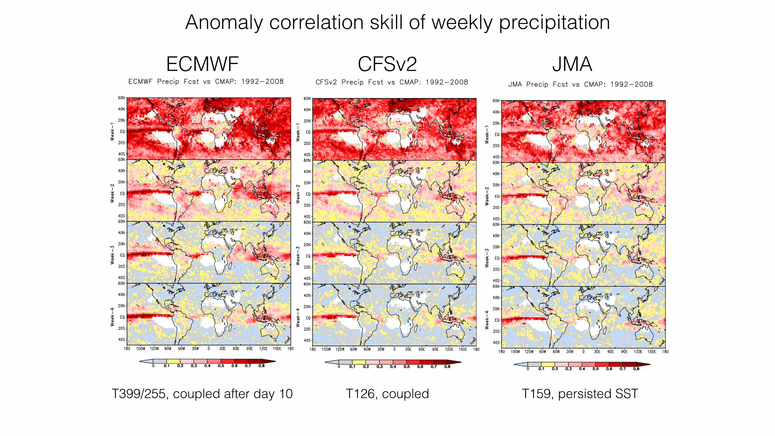
CONCLUSIONS 1) All the three model hindcast sets indicate very good skill for the first week, and relatively good skill for the 2nd week over the tropics, but dramatically decreased skill for weeks 3 and 4 except the equatorial Pacific and maritime continent.

2) The ECMWF hindcast demonstrates noticeably better skill than the other two, especially for weeks 3 and 4.

3) The predictability of sub-monthly precipitation appears to connect with intra-seasonal MJO phase/strength and low-frequency ENSO variability.

Acknowledgments: We are grateful to the provision of the three EPS hindcast data sets, from the Japanese Meteorological Agency, the National Centers for Environmental Prediction, and the European Centre for Medium-range Weather Forecasts.

.

The prediction skill of precipitation over sub-monthly time scale is investigated based on hindcasts from three global ensemble prediction systems (EPS). The results valid for up to four weeks indicate good skill or predictability over some regions during the boreal summer monsoon season (e.g., June through September), particularly over southeastern Asia and the maritime continent. The hindcasts from all the three models correspond to high predictability over the first week compared to the following three weeks. The ECMWF forecast system tends to yield higher prediction skill than the other two systems, in terms of both anomaly correlation and mean squared skill score. The sources of sub-monthly predictability are examined over the maritime continent with focus on the intra-seasonal MJO and interannual ENSO phenomena. Rainfall variations for neutral-ENSO years are found to correspond well with the dominant MJO phase, whereas for moderate/strong ENSO events, the relationship of rainfall anomaly with MJO appears to become weaker, while the contribution of ENSO to the sub-monthly skill is substantial. However, there is exception that if a moderate/strong MJO event propagates from Indian Ocean to the maritime continent during typical ENSO years, the MJO impact can become overwhelming, regardless of how strong the ENSO event is. These results support the concept that “windows of opportunity” of high forecast skill exist as a function of ENSO and the MJO in certain locations and seasons, that may lead to subseasonal to seasonal forecasts of substantial societal value in the future.

Evaluation of Sub-monthly Forecast Skill from Global Ensemble Prediction Systems Shuhua Li and Andrew W. Robertson

International Research Institute for Climate and Society, The Earth Institute at Columbia University, Palisades, NY 10964 (shuhua@iri.columbia.edu)

A13E–0259

FIGURE 4: Real-time MJO phase space during June 1 to Sept. 30 for 2002 (El Nino) and 2001(neutral-ENSO).

MJO phase: Jun – Sep, 2002 & 2001

• Hindcasts of precipitation from three global ensemble prediction systems over the common period 1992-2008: JMA long-range forecasting model, NCEP CFS version 2, and ECMWF integrated forecast system (IFS). • Horizontal resolution: approximately 1.125, 0.94, 0.5 degrees; and ensemble size: 5-4-5, respectively. • CMAP precipitation data from NOAA Climate Prediction Center. • Two skill metrics – Anomaly Correlation Coefficients (ACC) and Mean Square Skill Score (MSSS).

Linkage: Precip versus ENSO and MJO FIGURE 3: (a) Anomaly correlation between CMAP pentad precipitation and 5-day average Real-time Multi-variate MJO (RMM) during June to August, 1992-2008. It demonstrates high (negative) correlation of rainfall with RMM components over the maritime continent. (b) Correlations between ECMWF precipitation hindcast for week-3 and CMAP rainfall during 5 ENSO years (top) and 5 neutral years (bottom). The impact of ENSO on rainfall predictability is manifested by the comparison in the tropics, in particular over the equatorial Pacific and the maritime continent.

Precip time-series: ECMWF hindcast vs CMAP

FIGURE 5: Time series of rainfall anomalies over a portion of Borneo Island, from CMAP precipitation data (blue) and ECMWF hindcast (red), valid for weeks 2 and 3 during Jun-Sep for El Nino year 2002 and neutral-ENSO year 2001, respectively. The single upper-case letters denote the dominant MJO phase sector (A, I, M, P for MJO phase 8-1, 2-3, 4-5, and 6-7, respectively), where the MJO strength is greater than 1.0.

Global EPS and Precipitation Data

FIGURE 1: Correlation skill maps of precipitation hindcasts from the ECMWF forecast system over the period 1992–2008. The ACC calculations are made based on all the starts during late May through mid-September, and valid for weeks 1-4. Among the three global EPS, the ECMWF displays generally higher ACC skill than the other two systems, especially over the tropics and the maritime continent for weeks 2-4, as shown below.

ACC Skill Map from ECMWF: Precipitation Hindcasts (weeks 1-4) and CMAP Data

FIGURE 2: Aggregate ACC skill from three EPS hindcasts over the tropics and southeastern Asia

((a) (b)

A

I

M

P

Weekly average precip

Jun–Aug anomaly correlation

skill

Lead-dependent climos subtracted

skill from MJO and

atmos BCs}Li and Robertson (2015)

skill from atmos ICs

degrees of freedom, a CORA value of 0.2 is highly sta-tistically significant, with a p value of 0.003 shown aspink areas in Figs. 1–3.The CORA distribution for the CFSv2 and ECMWF

precipitation forecasts exhibit most of the above char-acteristics (Figs. 2 and 3). However, the CORA skill ofECMWF is notably higher than the other two models,

especially over the tropics for weeks 2–4. Indeed, relativelyhigh CORA values over the tropical Pacific resemblea slightly broader ITCZ-like characteristic than thatfrom JMA or CFSv2. The high CORA feature from theECMWF precipitation hindcast is also seen over theequatorial Atlantic and tropical Indian Ocean, as well asthe Maritime Continent (Fig. 3), where higher CORA

FIG. 2. As in Fig. 1, but for the CFSv2 hindcast.

JULY 2015 L I AND ROBERT SON 2875

exists compared to the JMAandCFSv2 hindcasts. Thesedominant characteristics will be further discussed in thenext section based on aggregate CORA skill over thetropical land area only and a specific region of interest,the Maritime Continent.Skill levels over the continents are generally disap-

pointing especially in weeks 3–4, although the ECMWFmodel does exhibit substantial skill at week 2 over South

America, Eurasia, and Australia. The rapidly decreasedskill level beyond one week in the extratropics is gener-ally consistent with the skill analysis using the PredictiveOcean Atmosphere Model for Australia (POAMA)coupled system (Zhu et al. 2014). Skill levels over Africaare poor even in week 1, which suggests that the ob-servational data quality may be poor on the weekly timescale. This could also be due to less predictability in that

FIG. 3. As in Fig. 1, but for the ECMWF hindcast.

2876 MONTHLY WEATHER REV IEW VOLUME 143

Anomaly correlation skill of weekly precipitation

maps. The correlation skill is generally very high duringthe first week and drops rapidly in most regions in thesubsequent three weeks. Nevertheless, there is consis-tently high CORA for all the leads, or weeks 1–4, overthe equatorial Pacific, located to the south of the

intertropical convergence zone (ITCZ). Weeks 2–4 alsoexhibit relatively higher skills (0.2–0.3) over the tropicalAtlantic, and the Maritime Continent. The 13 hindcastsper year over 17 years yields a very large sample size of221 hindcasts. Using a two-sided Student’s t test with 220

FIG. 1. Correlation of anomalies between JMA model precipitation hindcast and CMAPrainfall data for weeks 1–4 during the period 1992–2008. The white areas denote dry maskduring the June–September season, where the total CMAP rainfall over 122 days is lessthan 20mm.

2874 MONTHLY WEATHER REV IEW VOLUME 143ECMWF CFSv2 JMA

T399/255, coupled after day 10 T126, coupled T159, persisted SST

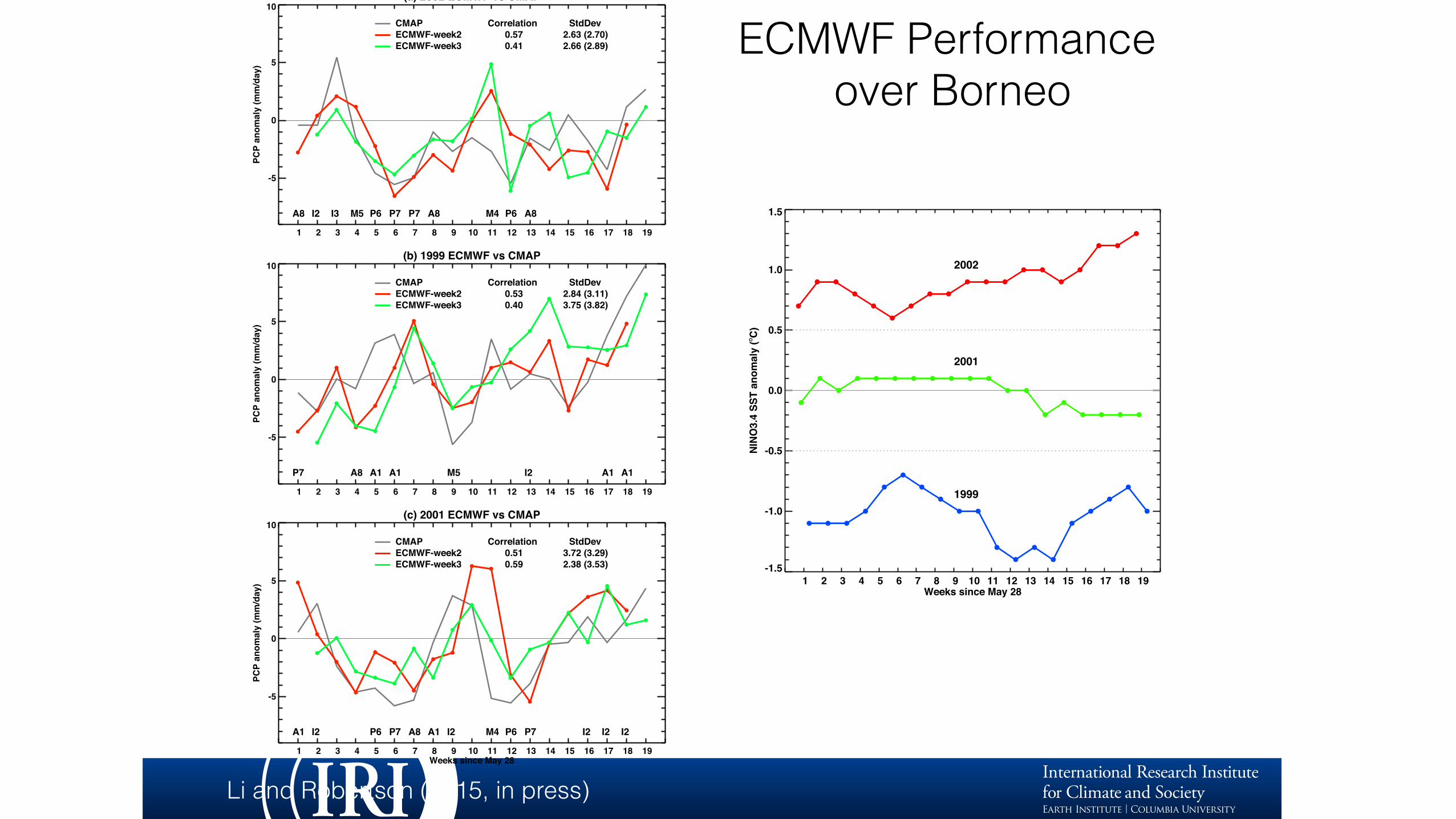
ECMWF Performance over Borneo

(a) 2002 ECMWF vs CMAP

1 2 3 4 5 6 7 8 9 10 11 12 13 14 15 16 17 18 19

-5

0

5

10

PCP

anom

aly

(mm

/day

)

A8 I2 I3 M5 P6 P7 P7 A8 M4 P6 A8

CMAPECMWF-week2ECMWF-week3

Correlation0.570.41

StdDev2.63 (2.70)2.66 (2.89)

(b) 1999 ECMWF vs CMAP

1 2 3 4 5 6 7 8 9 10 11 12 13 14 15 16 17 18 19

-5

0

5

10PC

P an

omal

y (m

m/d

ay)

P7 A8 A1 A1 M5 I2 A1 A1

CMAPECMWF-week2ECMWF-week3

Correlation0.530.40

StdDev2.84 (3.11)3.75 (3.82)

(c) 2001 ECMWF vs CMAP

1 2 3 4 5 6 7 8 9 10 11 12 13 14 15 16 17 18 19 Weeks since May 28

-5

0

5

10

PCP

anom

aly

(mm

/day

)

A1 I2 P6 P7 A8 A1 I2 M4 P6 P7 I2 I2 I2

CMAPECMWF-week2ECMWF-week3

Correlation0.510.59

StdDev3.72 (3.29)2.38 (3.53)

Figure 12: Time series of precipitation anomalies (mm/day) over a portion of Borneo Island,

from the CMAP data and ECMWF hindcast, valid for weeks 2 and 3 during June–September

for (a) 2002, (b) 1999, and (c) 2001, respectively. The upper-case letters along with single

digit at the bottom of each panel denote the dominant MJO phase sector and phase number

(see the text for detail), with amplitude greater than 1.0 (Wheeler and Hendon 2004). Along

the abscissa, weeks 1–5 correspond approximately to June; weeks 6–10 to July; weeks 11–14

to August; weeks 15–18 to September; and week 19 to Oct 1–7. Correlation values with

CMAP are given in each panel, together with the respective standard deviations, with the

CMAP values in parentheses. 48

Li and Robertson (2015, in press)

Weeks since May 28

(RMM1, RMM2) phase space for 1 Jun to 30 Sep 2002

-4 -2 0 2 4RMM1

-4

-2

0

2

4

RMM

2

12

34

56 7 8

9 101112 13

14 15

16

1718

1920

2122

23

2425

26272829

301

234567

8

910

111213

141516

171819

20 212223 2425262728

2930311

23 45 6

7

891011

12

13

14151617

1819202122

232425262728

293031 12345

6

78 9101112

131415

161718

19

20

2122

23242526

2728

2930

1

2 3

4

5

67

8

IndianOcean

Maritim

eContinent

WesternPacific

Wes

t Hem

.an

d Af

rica

Labeled dots for each day.Blue for Jun, orange for Jul, green for Aug, and red for Sep.

Figure 10: Real-time Multi-variate MJO (RMM) phase space (Wheeler and Hendon, 2004)

for June 01 through September 30, 2002, a typical year of El Nino.

45

June July

ECMWF Performance over Borneo

(a) 2002 ECMWF vs CMAP

1 2 3 4 5 6 7 8 9 10 11 12 13 14 15 16 17 18 19

-5

0

5

10

PCP

anom

aly

(mm

/day

)

A8 I2 I3 M5 P6 P7 P7 A8 M4 P6 A8

CMAPECMWF-week2ECMWF-week3

Correlation0.570.41

StdDev2.63 (2.70)2.66 (2.89)

(b) 1999 ECMWF vs CMAP

1 2 3 4 5 6 7 8 9 10 11 12 13 14 15 16 17 18 19

-5

0

5

10PC

P an

omal

y (m

m/d

ay)

P7 A8 A1 A1 M5 I2 A1 A1

CMAPECMWF-week2ECMWF-week3

Correlation0.530.40

StdDev2.84 (3.11)3.75 (3.82)

(c) 2001 ECMWF vs CMAP

1 2 3 4 5 6 7 8 9 10 11 12 13 14 15 16 17 18 19 Weeks since May 28

-5

0

5

10

PCP

anom

aly

(mm

/day

)

A1 I2 P6 P7 A8 A1 I2 M4 P6 P7 I2 I2 I2

CMAPECMWF-week2ECMWF-week3

Correlation0.510.59

StdDev3.72 (3.29)2.38 (3.53)

Figure 12: Time series of precipitation anomalies (mm/day) over a portion of Borneo Island,

from the CMAP data and ECMWF hindcast, valid for weeks 2 and 3 during June–September

for (a) 2002, (b) 1999, and (c) 2001, respectively. The upper-case letters along with single

digit at the bottom of each panel denote the dominant MJO phase sector and phase number

(see the text for detail), with amplitude greater than 1.0 (Wheeler and Hendon 2004). Along

the abscissa, weeks 1–5 correspond approximately to June; weeks 6–10 to July; weeks 11–14

to August; weeks 15–18 to September; and week 19 to Oct 1–7. Correlation values with

CMAP are given in each panel, together with the respective standard deviations, with the

CMAP values in parentheses. 48

Li and Robertson (2015, in press)

1 2 3 4 5 6 7 8 9 10 11 12 13 14 15 16 17 18 19 Weeks since May 28

-1.5

-1.0

-0.5

0.0

0.5

1.0

1.5

NINO

3.4

SST

anom

aly

(OC)

1999

2001

2002

Figure 11: Time series of observed weekly NINO3.4 index during late May through late

Septembet for three years, 2002, 1999, and 2001, as sampling years of El Nino, La Nina and

neutral ENSO conditions, respectively. The X-axis denotes week numbers since May 28, but

the ENSO index has minor shift of -2, -1 and +2 days for those three years.

46

12

Time-range

Resol. Ens. Size Freq. Hcsts Hcst length Hcst Freq Hcst Size

ECMWF D 0-32 T639/319L91 51 2/week On the fly Past 18y 2/weekly 11

UKMO D 0-60 N96L85 4 daily On the fly 1989-2003 4/month 3

NCEP D 0-45 N126L64 4 4/daily Fix 1999-2010 4/daily 1

EC D 0-35 0.6x0.6L40 21 weekly On the fly Past 15y weekly 4

CAWCR D 0-60 T47L17 33 weekly Fix 1981-2013 6/month 33

JMA D 0-34 T159L60 50 weekly Fix 1979-2009 3/month 5

KMA D 0-60 N216L85 4 daily On the fly 1996-2009 4/month 3

CMA D 0-45 T106L40 4 daily Fix 1992-now daily 4

Met.Fr D 0-60 T127L31 51 monthly Fix 1981-2005 monthly 11

CNR D 0-32 0.75x0.56 L54 40 weekly Fix 1981-2010 6/month 1

HMCR D 0-63 1.1x1.4 L28 20 weekly Fix 1981-2010 weekly 10

S2S partners

Probabilistic Verification:

Was this a good forecast?

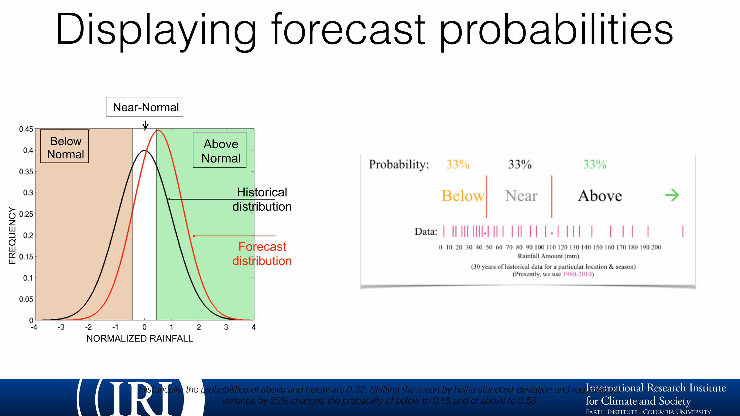
Below Normal

Above Normal

Historically, the probabilities of above and below are 0.33. Shifting the mean by half a standard-deviation and reducing the variance by 20% changes the probability of below to 0.15 and of above to 0.53.

Historical distribution

Forecast distribution

(Courtesy Mike Tippett)

Displaying forecast probabilitiesNear-Normal

NORMALIZED RAINFALL

FRE

QU

EN

CY

Validation of a single probabilistic forecast

Forecast PDF Verifying observation

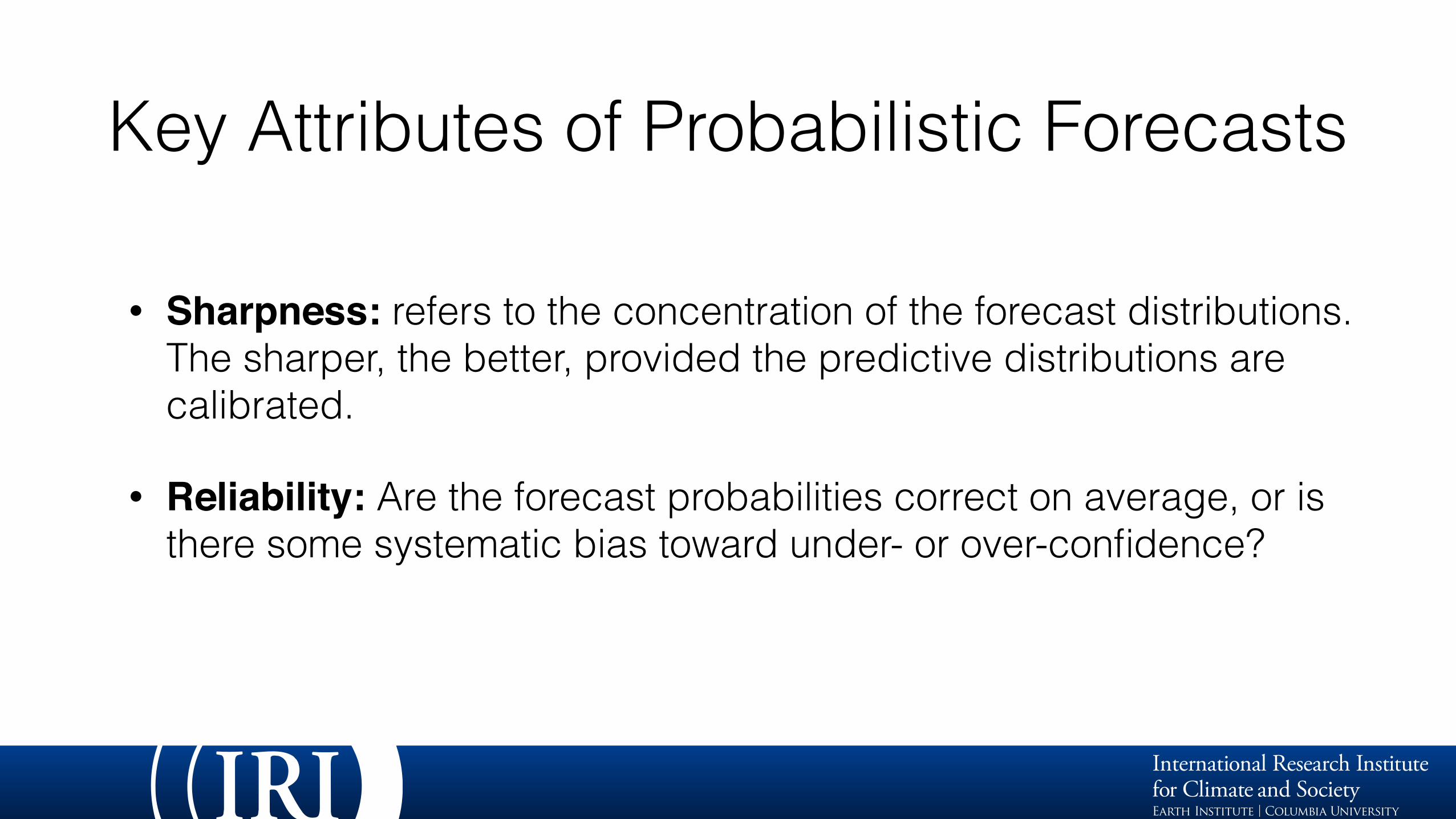
Key Attributes of Probabilistic Forecasts

• Sharpness: refers to the concentration of the forecast distributions. The sharper, the better, provided the predictive distributions are calibrated.

• Reliability: Are the forecast probabilities correct on average, or is there some systematic bias toward under- or over-confidence?

Reliability• Did we correctly indicate the

uncertainty in the forecast?

• Shows how well the forecast probabilities correspond to the subsequent observed relative frequencies of occurrence, across the full range of issued forecast probabilities

• The issued probabilities (from hindcasts) have to be binned, eg 0.45-0.55, 0.55-0.65, etc, so need long hindcast sets and pooling over space

This set of forecasts is well calibrated!

IRI Real-time Forecast Reliability

Sharpness• Sharpness measures whether the

forecasts vary much from the climatological distribution.

• Most seasonal forecasts avoid being overly precise (3, or maybe 5, categories).

• If probabilities near 0 and 1 (100%) are used often, then the forecast is said to be sharp. If most of the forecast probabilities are in the range 40 to 60% then this forecast system would be said to be "smooth" or "not sharp” (as on right).

frequency of issuance of each probability interval for each of the forecast categories

Jul-Aug-Sep (1950-1995)

Jul-Aug-Sep (1950-1995)

Above-Normal Below-Normal

Forecast probabilityForecast probability

Obs

erve

d re

lative

Fre

q.

Obs

erve

d re

lative

Fre

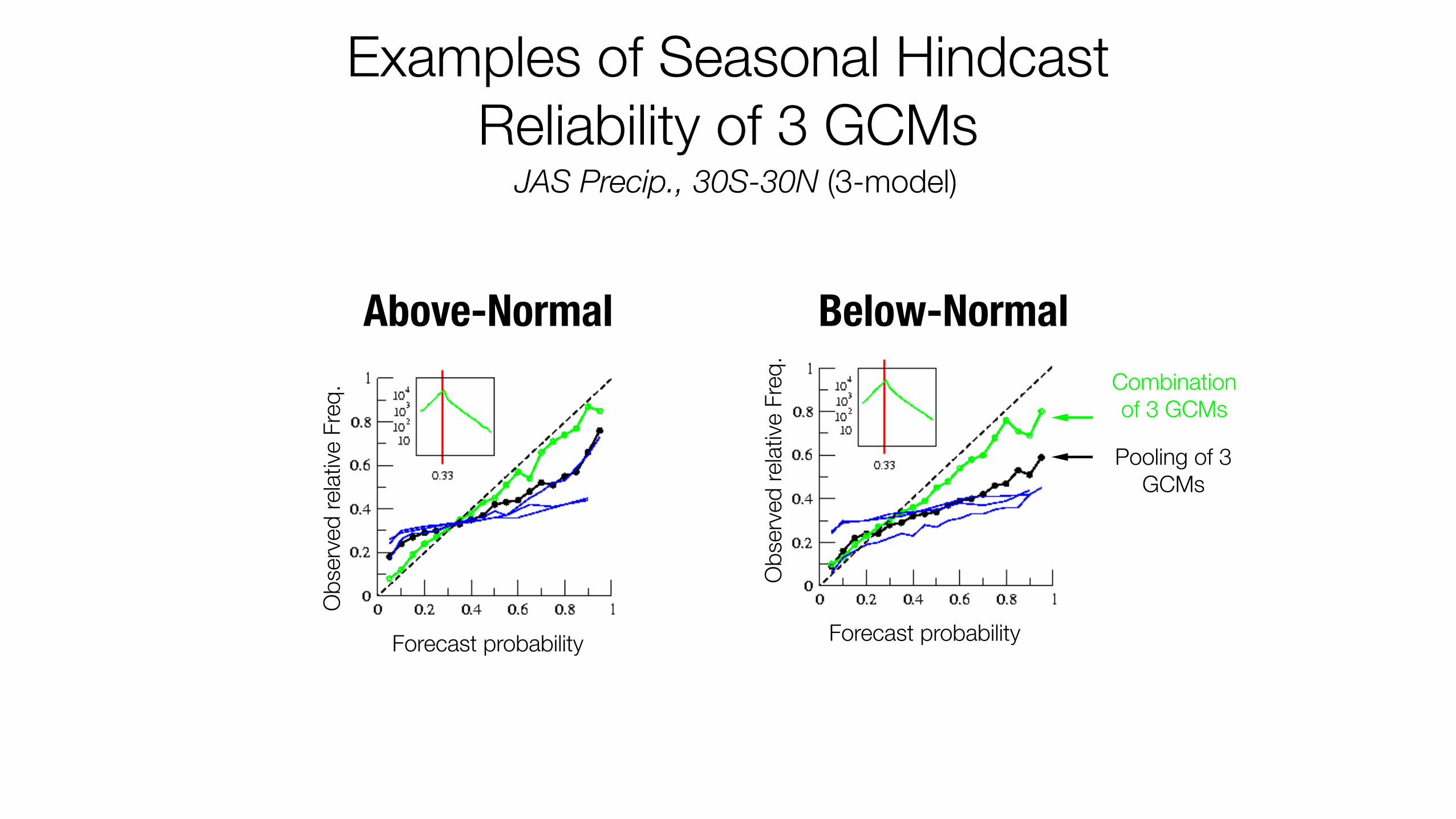
q. Combination of 3 GCMs

Pooling of 3 GCMs

JAS Precip., 30S-30N (3-model)

Examples of Seasonal Hindcast Reliability of 3 GCMs

S2S Sub-project on verification and products: Science questions

• What forecast quality attributes are important when verifying S2S forecasts and how they should be assessed?

Which verification methods and forecast attributes are appropriate for reporting S2S forecast quality to users, and which provide added insight into forecast system development and improvement?

• How should issues of short hindcast period availability and reduced number of ensemble members in hindcasts compared to real-time forecasts be dealt with when constructing probabilistic skill measures?

• How can we best identify windows of forecast opportunity, including assessing the contributions of climate drivers, such as the MJO and ENSO, to S2S forecast skill (e.g. consider skill assessment conditioned on ENSO phases)?

• Which verification methods are most appropriate for the verification of extreme events, particularly given challenges associated with their rarity, small sample sizes and large uncertainties?

• How can we best verify active and break rainfall phases and wet/dry spells in current S2S forecast systems?

• How can we best address verification in a seamless manner, for comparing forecasts across timescales?

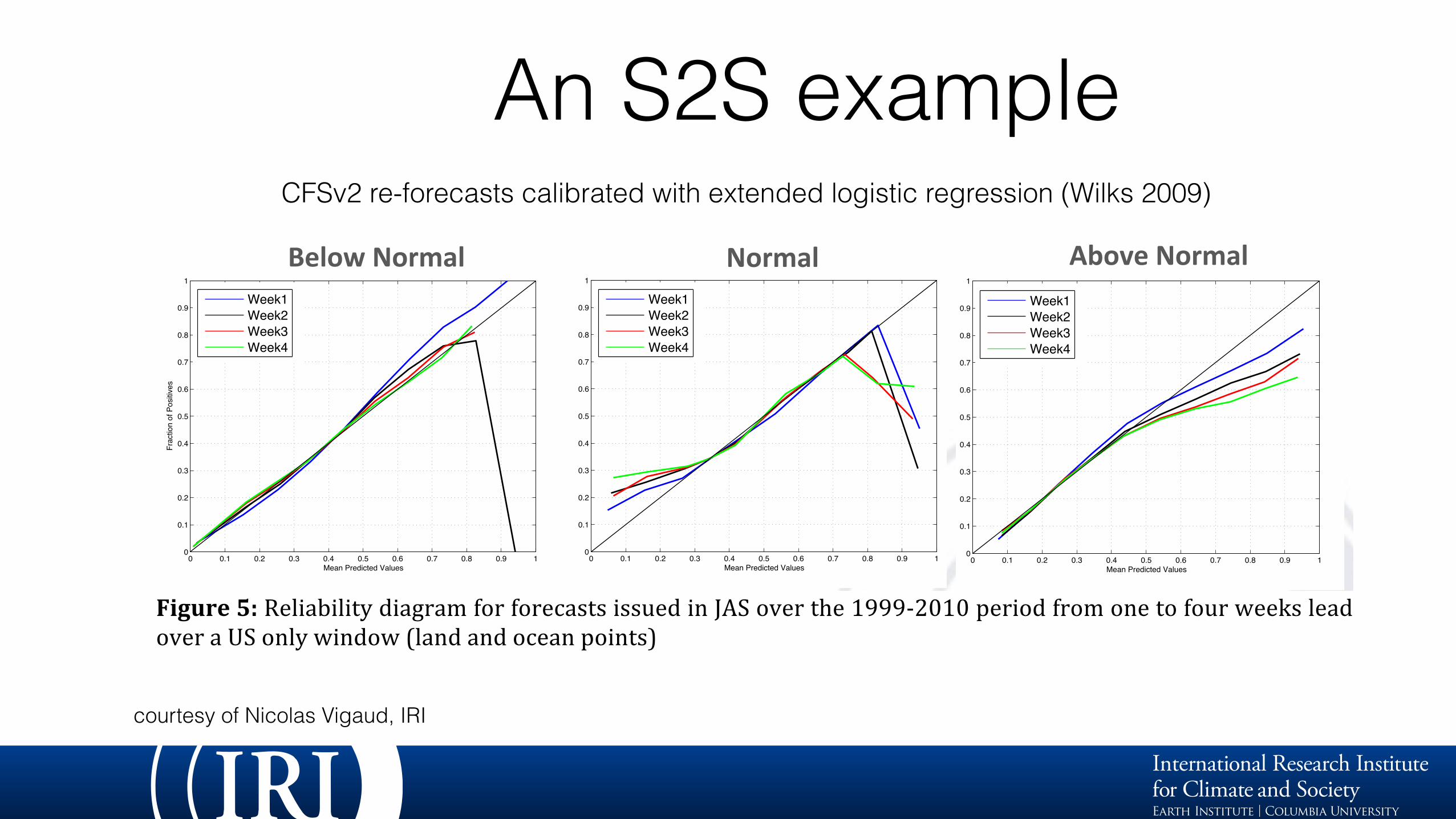
An S2S example

! "!

!"# $%&''()*+,-*./-#$01)2#./%!,+/#3&%/!*'.#4%&5*5,+,.,/'6#7888(2979#:;1#'.*%.'#!#$%&''()! *+,--./&'$0&120! 12+*$'2! 3+,4&4$'$1$2-! 5+,6! &''! -1&+1-! ,5! 7#8! 9.62642+-!+25,+2*&-1-! 5+,6! :;'(! 1,! 82312642+! ,/2+! 1<2! =<,'2! >???.@A>A! 32+$,0! &+2! %,=!*,%-$02+20B!#$C;+2!D!3+2-2%1-!1<2!-E$''!&--,*$&120!=$1<!2&*<!*&12C,+(!5+,6!&''!-1&+1-!,5!1<2!:F8!-2&-,%!5+,6!>???!1,!@A>A)!*,63;120!$%!&!-$6$'&+!*+,--./&'$0&120!6&%%2+B!G<2!+2'$&4$'$1(!5,+!2&*<!*&12C,+(!$-!&C&$%!2%*,;+&C$%C)!&%0!%&1;+&''(!02*+2&-2-!5+,6!=22E!>!1,!9!'2&0-B!!

!!"#$%&'()!H2'$&4$'$1(!0$&C+&6!5,+!5,+2*&-1-!$--;20!$%!:F8!,/2+!1<2!>???.@A>A!32+$,0!5+,6!,%2!1,!5,;+!=22E-!'2&0!,/2+!&!I8!,%'(!=$%0,=!J'&%0!&%0!,*2&%!3,$%1-K!

!!*+*' ,"-.$--"/0'102'3&%-3&.4"5&-'!L%!1<2!&33+,&*<!3+2-2%120!&4,/2)!1<2!2M12%020!',C$-1$*!+2C+2--$,%!6,02'!$-!4;$'1!$%!&!*+,--./&'$0&120!6&%%2+!;-$%C)!=$1<,;1!0$-*+$6$%&1$,%!&''!=22E-!5+,6!1<2!:F8!-2&-,%!5,+!0$552+2%1!=22E'(!+25,+2*&-1-B!!G<2!+2-;'1-!,41&$%20!&+2!+2&-,%&4'2!&%0!$'';-1+&12!1<2!+2'2/&%*2!,5!2M12%020!',C$-1$*!+2C+2--$,%!$%!1<2!8@8!*,%12M1B!!!!N,=2/2+)!1<2!-2&-,%&'$1(!=$1<$%!1<2!:F8!32+$,0!*,%-$02+20!$-!*'2&+'(!%,1!&**,;%120!5,+!&1!1<$-!-1&C2B!N2%*2)!&!%2M1!-123!=$''!*,%-$-1!$%!$%12C+&1$%C!=22E'(!-2&-,%&'$1(!$%!1<2!-1&1$-1$*&'!6,02'B!F6,%C-1!0$552+2%1!*<&''2%C2-)!1<2!>>!(2&+-!32+$,0!*,/2+20!4(!8@8! +25,+2*&-1-! *,;'0! 42! &%! ,4-1&*'2! 1,! *,63;12! +,4;-1! -1&1$-1$*-! &1!=22E'(! 1$62.-*&'2-B! O$552+2%1! &'12+%&1$/2-! =$''! 42! *,%-$02+20! 5+,6! &'12+%&1$/2! 12+*$'2-!*,63;1&1$,%! J-32*$5$*! 5,+! 2&*<! =22EK! 1,! C2,C+&3<$*&'! =2$C<1$%C! ,5! %2&+4(! C+$0.3,$%1-!1,!$%*+2&-2!1<2!3,,'!,5!1+&$%$%C!0&1&B!!!!6&7&%&0.&-'!N;556&%)!PB:B)!HB#B!F0'2+)!QB!Q,++$--2()!OBGB!R,'/$%)!8B!7;+1$-)!HB!:,(*2)!R!Q*P&/,*E)!:B!8;--E$%0! J@AA>K! P',4&'! S+2*$3$1&1$,%! &1! T%2.O2C+22! O&$'(! H2-,';1$,%! 5+,6!Q;'1$.8&12''$12!T4-2+/&1$,%-B!:"#<=-%&>/./&%B)!@)!U".DA!!

!e International Research Institutefor Climate and Society

0 0.1 0.2 0.3 0.4 0.5 0.6 0.7 0.8 0.9 10

0.1

0.2

0.3

0.4

0.5

0.6

0.7

0.8

0.9

1JAS 1999 2010 Above normal class

Mean Predicted Values

Frac

tion

of P

ositi

ves

0 0.1 0.2 0.3 0.4 0.5 0.6 0.7 0.8 0.9 10

0.1

0.2

0.3

0.4

0.5

0.6

0.7

0.8

0.9

1JAS 1999 2010 Normal class

Mean Predicted ValuesFr

actio

n of

Pos

itive

s0 0.1 0.2 0.3 0.4 0.5 0.6 0.7 0.8 0.9 1

0

0.1

0.2

0.3

0.4

0.5

0.6

0.7

0.8

0.9

1JAS 1999 2010 Below normal class

Mean Predicted Values

Frac

tion

of P

ositi

ves

!"#$%&$#$'()'"*'+),-.)/000123/3)45""6)/)'7)89)

:"#75);7<=%#) ;7<=%#) -&7>");7<=%#)

0 0.1 0.2 0.3 0.4 0.5 0.6 0.7 0.8 0.9 10

0.1

0.2

0.3

0.4

0.5

0.6

0.7

0.8

0.9

14 Jul 1999 A class

Mean Predicted Values

Frac

tion

of P

ositi

ves

Week1Week2Week3Week4

!"#$%#&'()*+,-(.#/*()**0(1,&234*5(6,%(#++('4#%4'(,6(4.*(789('*#',0'(6%,&(4.*(:;;;<=>:>(2*%",5(3'"0$(#++($%"52,"04'(-"4."0(4.*(?9(5,&#"0(@+*#/*<,0*<,34(1%,''</#+"5#A,0B(

(

(

(((

.6$##)?"@<"%*")%*)#"%?*)$A@<"%*")B<7=)5""6)2)&C')#"**)?"@<"%*")7A5%<?*)@7=D%<"?)'7)/000)%#7A")E"**"<)D"<B7<=%A@")B7<):"#75)A7<=%#)@#%**)4#$A6*)5$'F)#"**"<)7@@C<<"A@"*)7B)G3)<%$AH)?%(*)$A)IJK*L9)

0 0.1 0.2 0.3 0.4 0.5 0.6 0.7 0.8 0.9 10

0.1

0.2

0.3

0.4

0.5

0.6

0.7

0.8

0.9

14 Jul 1999 A class

Mean Predicted Values

Frac

tion

of P

ositi

ves

Week1Week2Week3Week4

0 0.1 0.2 0.3 0.4 0.5 0.6 0.7 0.8 0.9 10

0.1

0.2

0.3

0.4

0.5

0.6

0.7

0.8

0.9

14 Jul 1999 A class

Mean Predicted Values

Frac

tion

of P

ositi

ves

Week1Week2Week3Week4

0 0.1 0.2 0.3 0.4 0.5 0.6 0.7 0.8 0.9 10

0.1

0.2

0.3

0.4

0.5

0.6

0.7

0.8

0.9

14 Jul 1999 A class

Mean Predicted Values

Frac

tion

of P

ositi

ves

Week1Week2Week3Week4

courtesy of Nicolas Vigaud, IRI

CFSv2 re-forecasts calibrated with extended logistic regression (Wilks 2009)

Which Forecast Format?Daily weather Fcst

Week 3-4 Outlook

Seasonal Fcst

Summary of main points• Forecast verification requires large sets of forecasts of reforecasts/

hindcasts. This poses questions for S2S where the hindcast sets are shorter than typically for seasonal forecasts, and the ensemble sizes are reduced

• Verification of probabilistic forecasts involves considering many attributes of forecast quality. Reliability and sharpness are important attributes.

• Calibration intimately involves verification because it seeks to maximize sharpness while maintaining reliability. But re-forecast data must not be used twice!