Towards a regulatory framework for the use of liquid

hydrogen as a fuel for ships: Critical analysis of the

prescriptive requirements for bunkering operations

By

Johanne Charlotte Jakobsen

Master of Science – Process Safety Technology

Department of Physics and Technology

University of Bergen

June 2021

I

Acknowledgment

First, I would like to thank my main supervisor Dr Trygve Skjold for introducing me to the

topic of this thesis. His time, expertise and feedback has been very helpful throughout the

process. I would also express my gratitude to my co-supervisors Ivan Østvik, Kolbjørn Berge,

Veronica Charlotte Andersen Haugan, Melodia Lucas Pérez, Bjørn J. Arntzen and Helene

Hisken for meetings and advice during this period.

Furthermore, I would like to thank the people at Gexcon Fantoft that have been helping me with

the FLACS software and making room for me at the office. Your help is taken with great

gratitude.

Finally, I would like to thank my friends and family for their motivation and endless support

during this period.

II

Summary

The global demand for energy increases rapidly with the growth in the population and a steady

increase in the general standard of living. At the same time, the consumption of fossil fuels

causes massive releases of greenhouse gases (GHG) that influence the global climate. Hence,

the global energy mix needs a shift towards increasing use of renewable energy sources and

sustainable use of conventional fuels. In this perspective, various energy forecasts and strategies

outline a future where hydrogen and hydrogen-based fuels (including ammonia) will play an

important role as an energy carrier in industry and society.

In various parts of the maritime sector, liquid hydrogen (LH2) can replace conventional fuels

such as liquid natural gas (LNG) and marine fuel oils. Provided enough hydrogen can be

produced from renewable sources, or from fossil fuels with carbon capture, it will be possible

to reduce the GHG emissions from maritime transport significantly. However, a comparison of

critical safety-related properties of different fuels shows that it is not straightforward to achieve

the same level of safety for hydrogen systems, compared to conventional fuels.

Compared to LNG, LH2 has significantly lower storage temperature, much lower minimum

ignition energy (MIE), significantly wider flammable range, and much higher reactivity. Of

particular importance for safety distances related to fuel storage facilities and bunkering

operations is the propensity of hydrogen-air mixtures to undergo deflagration-to-detonation-

transition (DDT) under specific conditions. In summary, this implies a need for a different

approach to safety engineering, including the methods used for estimating safety zones for

bunkering operations. On the other hand, the low density and enthalpy of vaporisation of

hydrogen imply that accidental releases in the open often will be dominated by buoyancy, which

would be favourable from the point of view of safety.

Experimental data from large-scale releases of LH2 in the open are scarce. However, in 2019

the Norwegian Public Roads Administration (NPRA) and the Norwegian Defence Research

Establishment (FFI) commissions a series of controlled release and dispersion experiments with

LH2 from DNV GL. The experiments, performed at the large-scale test site at Spadeadam,

included seven outdoor tests representative of accident scenarios during bunkering operations.

The data from the tests document the size, shape and behaviour of the dispersed clouds

generated for specific tank pressures, outflow rates, and weather conditions.

This thesis explores safety challenges for bunkering operations and other operations involving

transfer of LH2 between or from cryogenic storage units. The aim is to provide science-based

III

recommendations for relevant regulations, codes and standards (RCS). The approach adopted

entails numerical simulations of the DNV GL experiments, to build confidence in the predictive

capabilities of the computational fluid dynamics (CFD) tool FLACS developed by Gexcon. The

FLACS software is then used to simulate hypothetical accident scenarios involving LH2. The

simulations focus on the formation and duration of flammable gas clouds near ground, without

ignition. The analysis includes a sensitivity study to explore the relative effect of selected

parameters on the size and shape of the dispersion clouds. Finally, the results from the

simulations are used to evaluate prescriptive requirements for LH2 bunkering operations in the

International Code of Safety for Ships using Gases or other Low-flashpoint Fuels (IGF Code)

from the International Maritime Organisation (IMO) and other relevant RCS. Notably, the IGF

Code only applies to the ship, including onboard bunkering stations, while standards such as

Ships and marine technology – Specification for bunkering of liquefied natural gas fuelled

vessels (ISO 20519) from the International Organization for Standardization (ISO) applies to

onshore bunkering operations in ports and harbours.

The results from both experiments and simulations show that parameters such as wind velocity,

release rate, release direction and outdoor temperature have significant impact on the dispersed

cloud. However, for similar conditions, a release of LH2 extends further than a release of LNG,

compared to earlier studies of LNG releases. Considering the ignition sensitivity and

significantly higher reactivity, including the propensity for DDT, for hydrogen compared to

methane, it is clear that releases of LH2 are more hazardous compared to releases of LNG.

Hence, to achieve the same level of safety, assuming similar leak rates and leak frequencies,

the safety distances, or safety zones, should be increased significantly in the case of LH2,

compared with LNG.

IV

Abbreviations

3D Three-dimensional

AIT Auto-ignition temperature

CCS Carbon capture and storage

CNG Compressed natural gas

DDT Deflagration-to-detonation-transition

DNS Direct numerical simulation

DSB The Norwegian Directorate for Civil Protection

FFI Norwegian Defence Research Establishment

GH2 Gaseous hydrogen, or compressed hydrogen

GHG Greenhouse gases

HAZID Hazard identification

HHV Higher heating value

IMO International Maritime Organization

ISO International Organization for Standardization

LES Large eddy simulation

LFF Low flash point fuel

LFL Lower flammability limit

LH2 Liquid hydrogen

LHV Lower heating value

LNG Liquid natural gas

LOHC Liquid organic hydrogen carrier

LPG Liquid petroleum gas

MESG Maximum experimental safe gap

MIE Minimum ignition energy

NMA Norwegian Maritime Authority

NPRA Norwegian Public Roads Administration

PPE Personal protective equipment

QD Quenching distance

QRA Quantitative risk assessment

RANS Reynolds-averaged Navier-Stokes

RCS Regulations, codes and standards

SOLAS Safety Of Life At Sea

V

Contents

Acknowledgment ...................................................................................................................... I

Summary .................................................................................................................................. II

Abbreviations .......................................................................................................................... IV

1. Introduction ...................................................................................................................... 1

1.1 The role of hydrogen in maritime transport ............................................................... 1

1.2 Safe implementation of hydrogen for maritime systems............................................ 3

1.3 Approach .................................................................................................................... 5

1.4 Objectives ................................................................................................................... 5

1.5 Outline of thesis.......................................................................................................... 5

2. Background ....................................................................................................................... 7

2.1 Why hydrogen? .......................................................................................................... 7

2.1.1 Liquid hydrogen ..................................................................................................... 8

2.1.2 Release of liquid hydrogen ..................................................................................... 8

2.2 Characteristics of hydrogen that cause safety challenges .......................................... 8

2.2.1 Storing pressure ...................................................................................................... 9

2.2.2 Boiling point ......................................................................................................... 10

2.2.3 Flammable limits .................................................................................................. 10

2.2.4 Ignition sensitivity ................................................................................................ 10

2.2.5 Reactivity.............................................................................................................. 11

2.2.6 Embrittlement ....................................................................................................... 12

2.2.7 Emerging technologies and strength of knowledge ............................................. 12

2.3 Characteristics of hydrogen that may be favourable ................................................ 12

2.4 Basics aspects of risk assessments ........................................................................... 13

2.6 The IGF Code ........................................................................................................... 15

2.7 Bunkering and safety zones ...................................................................................... 15

3. Literature review ............................................................................................................ 17

3.1 Experimental findings of liquid hydrogen release in open rooms............................ 17

3.1.1 General description of experiment ....................................................................... 17

3.1.2 Dispersion mechanisms of the H2 flammable cloud ............................................ 18

3.1.3 Conclusion of the NASA experiments ................................................................. 19

3.2 Ignited releases of liquid hydrogen .......................................................................... 20

3.2.1 Thermal of safety distances .................................................................................. 20

VI

3.3 Liquid hydrogen releases show dense gas behaviour. .............................................. 21

3.3.1 Background - Liquid release of hydrogen ............................................................ 21

3.3.2 Bunkering ............................................................................................................. 22

3.3.3 Vent mast releases ................................................................................................ 23

3.3.4 Conclusion of the work ........................................................................................ 25

4. Experiments involving outdoor releases....................................................................... 26

4.1 Background for the experiment ................................................................................ 26

4.2 Description of experiments ...................................................................................... 26

4.2.1 Measurements of Ambient Conditions ................................................................. 28

4.2.2 Dispersion Measurements .................................................................................... 29

4.2.3 Ignition Measurements ......................................................................................... 30

4.3 Results summary from experiments ......................................................................... 30

4.3.1 Results Test 1 ....................................................................................................... 31

4.3.2 Results Test 2 ....................................................................................................... 31

4.3.3 Results Test 3 ....................................................................................................... 32

4.3.4 Results Test 4 ....................................................................................................... 33

4.3.5 Results Test 5 ....................................................................................................... 33

4.3.6 Results test 6 ......................................................................................................... 34

4.3.7 Results Test 7 ....................................................................................................... 35

4.4 Summary of the experimental results ....................................................................... 36

5. Methodology.................................................................................................................... 37

5.1 Background .............................................................................................................. 37

5.1.1 The governing equations ...................................................................................... 38

5.1.2 Turbulence models ............................................................................................... 39

5.1.7 The model system ................................................................................................. 40

5.1.8 Validation ............................................................................................................. 41

5.2 Model simplification and assumptions ..................................................................... 41

5.3 Simulation set-up ...................................................................................................... 42

5.3.1 Geometry .............................................................................................................. 42

5.3.2 Grid ....................................................................................................................... 43

5.3.3 Scenario ................................................................................................................ 43

5.3.4 Monitor Points ...................................................................................................... 43

5.3.5 Single field 3D output .......................................................................................... 43

5.3.6 Simulation and output control .............................................................................. 43

5.3.7 Boundary conditions............................................................................................. 44

5.3.8 Initial conditions ................................................................................................... 44

5.3.9 Gas composition and volume ............................................................................... 44

5.3.10 Gas monitor region ........................................................................................... 44

5.3.11 Leaks ................................................................................................................ 44

5.3.12 Wind ................................................................................................................. 44

VII

5.3.13 Ignition ............................................................................................................. 44

6. Results and discussion .................................................................................................... 45

6.1 Validation of FLACS-simulations compared to the experiments ............................ 45

6.1.1 Test 1, Release without increasing tanker pressure .............................................. 45

6.1.2 Test 2, Higher release rate and opposite wind direction ...................................... 47

6.1.3 Test 3, Higher outflow rate................................................................................... 47

6.1.4 Test 4, Horizontal release ..................................................................................... 49

6.1.5 Test 5, First ignited test, vertical downward release ............................................ 50

6.1.6 Test 6 Second ignited test, horizontal release ...................................................... 51

6.1.7 Test 7, Final release to empty tanker .................................................................... 52

6.1.8 Summary of the FLACS results ........................................................................... 53

6.2 The impact of changing essential parameters........................................................... 58

6.2.1 Wind velocity ....................................................................................................... 58

6.2.2 Pasquill classes ..................................................................................................... 61

6.2.3 Temperature.......................................................................................................... 62

6.2.4 Grid ....................................................................................................................... 64

6.2.5 Change of release orientation ............................................................................... 65

6.2.6 Adding barriers ..................................................................................................... 67

6.3 Are safety distances for LNG suitable for LH2? ...................................................... 70

7. Conclusions ..................................................................................................................... 72

7.1 Main conclusions ...................................................................................................... 72

7.2 Suggestions for further work .................................................................................... 72

Bibliography............................................................................................................................ 74

Appendix A: Coordinates for monitor points ...................................................................... 78

Appendix B – Results from experiments and simulations .................................................. 80

1

1. Introduction

1.1 The role of hydrogen in maritime transport

Energy technologies are important for everyday life. Consumption of energy has played a

crucial role for humankind since early humans learned how to control fire, and energy will

continue to play an essential role for the lives of our descendants. The demand for energy will

increase with the rapid increase in the global population, combined with increasingly developed

societies. The consumption of fossil fuels results in massive releases of greenhouse gases

(GHG), in particular carbon dioxide (CO2), that influence the environment and cause climate

change. Hence, the energy system needs a shift towards sustainable use of conventional fuels

and an increasing fraction of energy from renewable sources in the global energy mix.

However, the inherent variation in the energy production from solar and wind implies a need

for carbon-free energy carriers, such as hydrogen or hydrogen-based fuels (e.g., ammonia).

The International Energy Agency (IEA) reported that the global transport sector used 31 000

TWh in 2015, which constituted 14% of the global GHG emissions [1]. In April 2018, the

International Maritime Organization (IMO) decided to reduce GHG emissions by at least 50%

by 2050 [2], and the goal is to eventually reduce the emissions to zero. In addition to the global

emissions, there are also strong incentives to reduce the local emissions of GHG and other

pollutants. As an added measure to reduce the emission from maritime vessels, the Norwegian

Parliament has decided that ships and ferries in the world heritage fjords need to implement

zero-emission technology as soon as technical possible, and within 2026 [3].

Energy stored in batteries is a practical solution for ferries and other ships that travel relatively

short distances. One example is the world’s first electric car and passenger ferry MF “Ampere”,

trafficking European route E39 between Lavik and Oppedal. However, for long-distance freight

the size and weight of large battery assemblies represent a significant challenge. For this

segment, hydrogen technologies is a viable alternative to conventional fuels, such as marine

fuel oils and liquid natural gas (LNG). Maritime vessels powered by hydrogen system can

operate longer routs with lower vessel weight [4].

The maritime sector has several alternatives for sustainable replacement of conventional fuels,

including methanol, ethanol, ammonia, compressed hydrogen (GH2), liquid hydrogen (LH2)

2

and liquid organic hydrogen carriers (LOHC). Figure 1 compares different fuels based on the

gravimetric (specific) and volumetric energy densities. Hydrogen has significantly higher

energy density per unit mass compared to other fuels, including ammonia and methanol.

However, the volumetric energy density of hydrogen is low, even at high pressures or in liquid

(cryogenic) state. The higher volumetric energy density of LH2, compared to GH2, is

favourable for ships with high energy consumption [5].

Figure1: Energy densities for different fuels [6].

Hydrogen has both advantages and disadvantages as an energy carrier. The main advantage of

hydrogen is that it is a zero-carbon energy carrier, which implies no direct emissions of carbon

dioxide. The total GHG emissions will depend on how hydrogen is manufactured, and

combustion of hydrogen can also result in local pollution from NOx [7]. Most of the hydrogen

used today is manufactured by steam reforming of conventional fuels, such as coal, oil and

natural gas, without carbon capture. However, it is foreseen that an increasing fraction of the

hydrogen will be produces by electrolysis, using electricity generated from renewable energy

sources [8]. The main challenges towards realising the hydrogen economy include technology

development, implementation of infrastructure, costs, upscaling, availability and safety.

3

1.2 Safe implementation of hydrogen for maritime systems

This thesis evaluates safety challenges related to LH2 technologies for maritime applications,

with particular focus on safety for operations in unconfined settings, such as bunkering of

maritime vessels or transfer of LH2 from cryogenic tanks on deck to consumers such as fuel

cells or turbines. The work progressed in parallel with another thesis that focused on LH2

operations in confined settings, such as fuel preparation rooms and fuel cell rooms.

Ships that are in operation today follow internationals regulations, codes and standards (RCS)

and codes to achieve a certain level of safety. In response to the Titanic disaster on 15 April

1912, the first SOLAS (Safety Of Life At Sea) treaty was established in 1914. This and later

treaties were established to increase the level of safety for ships by introducing minimum safety

standards for constructions, equipment and operations on board [9]. The International Maritime

Organization (IMO) was established in 1948. IMO issues international safety standard to

promote maritime safety, including comprehensive international regulations [10].

The International Code of Safety for Ships using Gases or other Low-flashpoint Fuels (IGF

Code) entered into force on 1 January 2017 [2]. This legislation was established to minimize

the risk for ships, their crews and the environment, given the nature of gaseous fuels relative to

conventional fuel oils [11]. The current version of the IGF Code provide mandatory provisions

for all fuels with flash point below 60 C (for the primary fuel), but specific requirements only

for natural gas, including LNG (Part A-1 of the IGF Code). For all other fuels with low flash

point, including hydrogen, the IGF Code and other documents from IMO prescribe functional

requirements for an Alternative Design process that entails an extensive risk assessment. For

instance, §3.2.1 of the IGF Code specifies [11]:

“The safety, reliability and dependability of the systems shall be equivalent to that achieved

with new and comparable conventional oil-fuelled main and auxiliary machinery.”

Since LH2 and LNG have some physical and combustion properties in common, including

similar lower flammability limits (LFL), similar auto ignition temperatures (AIT), and low

boiling points and flash points relative to ambient conditions, it could be tempting to apply

similar functional requirements for both fuels. However, there are also significant differences

between LH2 and LNG that might imply that more extensive safety measures will be required

for hydrogen to achieve equivalent levels of safety. The minimum ignition energy (MIE) of

hydrogen (≈0.017 mJ) is much lower than for methane (≈0.34 mJ), and hydrogen has a wider

4

range in flammable concentration (4-77 vol.%), compared to methane (5-15 vol.%) [12]. LH2

is stored at significantly lower temperatures (-253 C) compared to LNG (-162 C). Finally,

stoichiometric or worst-case hydrogen-air mixtures are dramatically more reactive than

methane-air mixtures. The maximum laminar burning velocity SL for hydrogen is about 2.9 m/s,

whereas the maximum laminar burning velocity of methane-air mixtures is about 0.36 m/s [12].

This has severe implications for the consequences of accidental explosions. Experiments in

specific open congested geometries with stoichiometric fuel-air mixtures show that hydrogen

produces significantly higher explosion pressures [13][14]. In summary, the safety-related

properties of hydrogen differ significantly from conventional fuels, implying that the functional

requirements in a prospective section for hydrogen in the IGF Code will have to differ

significantly from those for natural gas to achieve a comparable level of safety.

Compliance with the Alternative Design route prescribed by IMO [15], is particularly

challenging for the emerging hydrogen technologies, where the inherent lack of relevant

experience implies significant uncertainty in any estimate of event frequencies. Furthermore,

the results from a recent blind-prediction benchmark study for vented hydrogen deflagrations

in 20-foot shipping containers demonstrate a severe lack of predictive capabilities for advanced

consequence models [16]. The weak strength of knowledge in risk assessments for hydrogen

systems implies that any quantitative assessment of risk will entail significant uncertainties

[14]. This should be reflected in the way results from quantitative risk assessments (QRAs) are

used to support decisions concerning the design and operation of hydrogen systems, including

ships and bunkering systems in ports and harbours.

There is currently no standard or regulation that specify functional requirements for the use of

hydrogen as fuel in the maritime transport sector. Hence, the main motivation for the work

presented in thesis is to investigate specific challenges concerning the safe use of hydrogen as

an energy carrier for ships. In particular, the thesis explores the relative level of safety for

systems based on LH2 and LNG, with a view to propose recommendations for a prospective

revision of the IGF Code and related standards that will include functional requirements for

hydrogen, including LH2. The IGF Code applies to on-board bunkering station, while ISO

20519 [17] “Gas as a marine fuel ‒ Controlled Zones during LNG bunkering” [18] and the

guidelines from DNV GL “Recommended practise ‒ Development and operation of liquefied

natural gas bunkering facilities” [19] apply to bunkering operations on-shore. Finally, the

present work in limited to open congested geometries, such as bunkering systems. The thesis

5

of another Master student focused on confined systems, such as fuel preparation rooms, fuel

cell rooms and machinery spaces.

1.3 Approach

To gain more knowledge about the behaviour of liquid hydrogen (LH2) releases, DNV GL

Spadeadam Research and Testing performed a series of large-scale release and dispersion tests

commissioned by the Norwegian Defence Research Establishment (FFI) [20] on behalf of the

Norwegian Public Roads Administration (NPRA) and the Norwegian Maritime Authority

(NMA). The design of the experiments should replicate bunkering operations with large

accidental releases of LH2. The test series included seven experiments with variations in

storage pressure, release rate, release directions and weather conditions. As a part of the work

for this master thesis, the experiments were simulated with the computational fluid dynamics

(CFD) software FLACS to evaluate the predictive capabilities of the software. The same

software with similar settings were then used to simulate hypothetical accident scenarios, for a

range of parameters: release rates, temperatures, wind velocity etc. Finally, the results from the

CFD simulations inform a critical analysis of the applicability of existing RCS for bunkering

operations with LH2.

1.4 Objectives

The primary objective of this thesis is to determine whether and to what extent existing RCS

for bunkering operations involving LNG are applicable for bunkering operations involving

LH2. The secondary objectives are:

• To validate the CFD tool FLACS against large-scale release and dispersion experiments

with LH2 in the open.

• To provide general recommendations for RCS concerning LH2 bunkering operations.

1.5 Outline of thesis

Chapter 2 presents background information of hydrogen as an energy carrier, including a review

of safety-related properties of hydrogen and conventional fuels. Chapter 3 reviews previous

work on LH2 releases in the open. Chapter 4 summarises the large-scale release and dispersion

experiments with LH2 performed by DNV GL Spadeadam Research and Testing [20]. Chapter

5 describes the CFD simulations with FLACS, including simplifications and assumptions.

Chapter 6 presents the results from the simulation and discusses the implications for RCS,

6

including the effect of critical parameters. Finally, Chapter 7 summarises the main conclusions

and suggestions for further work.

7

2. Background

This chapter introduces hydrogen as an energy carrier and presents characteristic properties

of hydrogen that may cause safety challenges for ships fuelled by hydrogen in the maritime

transport sector.

2.1 Why hydrogen?

The maritime sector represents about 5% of the global oil demand today. Furthermore, it is

responsible for 2.5% of global energy-related CO2 emissions [21]. To reduce the emissions

from the maritime transport sector, new technology is required. Norway has already introduced

electric ferries as a means to reduce the emission of CO2 and other GHG. The first fully

electrical ferry, MF Ampere, was launched in 2015, and there are currently 34 electrical car

ferries in operations in Norwegian fjords [22]. However, battery technologies are not suitable

for all ships. For longer routes and larger ships, battery solutions are not viable solutions, partly

because of the considerable size and weight, and partly due to the time required for charging

the batteries. This is one of the motivating factors for considering hydrogen technologies as a

viable alternative to conventional fuels such as LNG, diesel and marine fuels oils. According

to Aarskog et al. [4]:

“A 250-350 bar hydrogen storage tank is about five times lighter than a maritime battery

system. A hydrogen system can result in longer range or lower ship weight, which makes

it an alternative for a wider range of applications”

Hydrogen is also a promising fuel for a sustainable future because of its low emission of GHG,

especially CO2.

Hydrogen is the first element in the periodic system, the lightest of all gases, and contains

more chemical energy per unit mass (MJ/kg) than natural gas and gasoline. The high energy

content combined with low CO2 footprint makes hydrogen an attractive energy carrier in the

transport sector. The low molecular weight implies that hydrogen has very low energy density

(MJ/m3) at ambient temperature and pressure. In practical energy systems, this can to some

extent be compensated by compressed storage at high pressures, typically 200-700 bar, or

liquefaction. At −252.87 °C (20.28 K), hydrogen is a stable cryogenic liquid at atmospheric

pressure. Alternative storage solutions include chemical compounds, such as ammonia or

8

liquid organic hydrogen carriers (LOHCs). The amount of pure hydrogen found in nature is

very limited, and for energy applications hydrogen must be manufactured from energy

sources. Hydrogen can for instance be produced from water (e.g., electrolysis), biomass (e.g.,

fermentation) and fossil fuels (e.g., steam methane reforming).

2.1.1 Liquid hydrogen

In the maritime sector liquid hydrogen seems to be the most advantageous way of storing

hydrogen when it comes to bunkering process as well as the preferred solution for vessels with

high power consumption [5]. When the hydrogen is stored as a liquid it has a higher volumetric

energy density compared to compressed hydrogen. Storing hydrogen as a cryogenic liquid

requires low temperatures (around 20-30 K) depending on the storage pressure (1-10 bar). In

addition to the high volumetric density, hydrogen has a higher gravimetric density than diesel,

gasoline, ammonia, methanol, and methane [6] and it is illustrated in Figure 1. This makes

hydrogen more efficient for storing, transport and distribution. However, the low temperature

requires a complex storing system and access of energy to achieve the low temperatures.

Storing hydrogen at 20 K would require about 25-35% of the hydrogen energy if the hydrogen

itself would supply the energy for cooling the storage system [21].

2.1.2 Release of liquid hydrogen

A release scenario of liquid hydrogen will depend on how it is stored and if the release scenario

is impinging, confined or in the open. Hydrogen has a low boiling point (20 K at atmospheric

pressure) and will rapidly evaporate when it is released in atmospheric conditions. Gaseous

hydrogen is significantly lighter than air and will have a higher velocity upward in the

atmosphere. The lower temperature for hydrogen causes a higher vaporizing compared with

LNG, because the attraction between the molecules is weaker for LH2 than for LNG. This will

be advantageous from a safety perspective if there was to be an accidental release of hydrogen.

Due to the higher vaporizing ability hydrogen will remain at ground level for a shorter time,

compared to a release of LNG.

2.2 Characteristics of hydrogen that cause safety challenges

Hydrogen has different characteristics than conventional fuels and might require different

standards to achieve a comparable safety level to the conventional energy carriers. Ships that

are in operation today and are fuelled with LNG follow standards from the IGF Code. In the

9

IGF Code part A – Alternative design (point 3.2.1) it says [11]: “The safety, reliability and

dependability of the systems shall be equivalent to that achieved with new and comparable

conventional oil-fuelled main and auxiliary machinery”. This means that hydrogen needs to

have a safety level that is comparable to the conventional fuels. Characteristics of hydrogen

compared with conventional fuels are listed in Table 2.1. The critical properties of hydrogen

when it comes to safety considerations will be discussed further.

Table 2.1 - Characteristic properties of hydrogen and conventional fuels [6], [12],[21],[23],[33]

2.2.1 Storing pressure

Property Hydrogen Conventional fuels

Higher heating

value (HHV) 142 MJ kg-1

Methane:

55 MJ kg-1

Propane:

50 MJ kg-1

Diesel/jet fuel:

45-46 MJ kg-1

Lower heating

value (LHV) 120 MJ kg-1

Methane:

50 MJ kg-1

Propane:

46 MJ kg-1

Diesel/jet fuel:

43 MJ kg-1

Storage and

transport pressure

(GH2)

700 bar

CNG:

260 bar

LPG:

30 bar

Marine gas oil, heavy fuel oil,

diesel and petrol are normally

stored at atmospheric pressure

Boiling point/

temp. for

transport and

storage

(LH2)

-253 C

LNG:

-162C

Propane:

-42C

Flash point (LH2)

< -253 C

LNG:

-188 C

LPG:

- 104 C

Marine fuel oil:

> 60 C

Flammable limits

(vol% fuel in air) 4-77

Methane:

5-15

Propane:

2.1 – 9.5

Minimum ignition

energy (MIE)

0.017 mJ

Methane:

0.28 mJ

Propane:

0.26 mJ

Auto ignition

temperature (AIT) 500 C

Natural gas:

640 C

Propane:

466 C

Maximum

experimental safe

gap (MESG)

0.29 mm Methane:

1.12 mm

Propane:

0.92 mm

Quenching

distance (QD) 0.64 mm 2.03 1.75

Maximum laminar

burning velocity in

air mixtures (SL)

2.9 m s-1 Methane:

0.36 m s-1

Propane:

0.41 m s-1

Enthalpy of

vaporisation, Hvap 0.92 kJ/mol

Methane:

8.17 kJ/mol

Propane:

15.7 kJ/mol

The detonation cell

size for stoich.

fuel-air mixture

10 mm Methane:

300 mm

Propane:

70 mm

10

Gaseous hydrogen (GH2) is often stored and transported at significantly higher pressures,

typically 350-700 bar, compared to other gaseous fuels. Compressed natural gas (CNG) and

liquefied petroleum gas (LPG) are typically stored at 260 and 30 bar, respectively, and tanks

for liquid fuels such as petrol, diesel and marine fuel oils will typically have atmospheric

pressure in the tank space. The high storage pressure for GH2 imply significant challenges

concerning the prevention of loss of containment, for instance cause by material or component

failure, and releases from high-pressure reservoirs will often be dominated by momentum, not

buoyancy.

2.2.2 Boiling point

Hydrogen has a very low boiling point (-253 C), and LH2 is therefore stored at much lower

temperatures than the conventional fuels, including LNG. Cryogenic storage and transport

require special materials and complex system for cooling. Loss of containment, and hence

insulation, of LH2 will result in flashing and further expansion as the temperature increases

above the boiling point. A particular concern concerning accidental releases of LH2 is the

possibility of condensing oxygen and nitrogen from the air. This can result in clogging of

hydrogen lines, as well as the formation of an explosive condensate consisting of hydrogen,

oxygen and nitrogen [23] [24].

2.2.3 Flammable limits

Whereas the lower flammability limit (LFL) of hydrogen (4.0 vol.% in air) is comparable to

propane (2.1 vol.%) and methane (5.0 vol.%), the upper flammability limit (UFL) for hydrogen

(75-77 vol.% in air) is much higher than for conventional fuels, including propane (9.5 vol.%)

and methane (15 vol.%). The wide flammable range implies that it is more challenging to

prevent the formation of explosive atmospheres [12].

2.2.4 Ignition sensitivity

Hydrogen has significantly lower minimum ignition energy (MIE ≈ 0.017 mJ), quenching

distance (QD ≈ 0.64 mm) and maximum experimental safe gap (MESG ≈ 0.29 mm), compared

to conventional energy carriers [12]. This implies that it is inherently difficult to prevent all

ignition sources. This means that ignition sources that do not represent a hazard for

conventional energy carriers, still can be a potential hazardous ignition source for hydrogen-air

mixtures. Hydrogen is classified in Gas Group IIC, together with acetylene, which implies

special requirements concerning electrical and non-electrical equipment. Finally, releases of

11

hydrogen from pressurised containers can under specific conditions result in spontaneous

ignition.

2.2.5 Reactivity

Hydrogen has significantly higher maximum laminar burning velocity (2.9 m/s), compared to

conventional fuels (Table 2.1). The laminar burning velocity SL is a fundamental parameter of

fuel-air mixtures. In principle, SL is the propagation velocity of a planar (unstretched) flame

front relative to the unburned mixture, for a specific pressure, temperature and fuel

concentration [12]. The high laminar burning velocity of hydrogen is caused by fast chemical

kinetics and high diffusivity.

A planar laminar flame is inherently difficult to realise in practice, partly due to flame stretch

and partly due to various instability phenomena. In practice, most accidental explosions entail

turbulent combustion, that under certain conditions can transition into detonations. A turbulent

flame will always propagate at significantly higher velocity, the so-called turbulent burning

velocity ST, compared to the theoretical value of SL for the same pressure, temperature and

mixture composition. Expansion, especially in partly confined systems, and flame folding and

generation of turbulence in the wakes of congestion, can result in flame acceleration and

pressure build-up, and under certain conditions deflagration-to-detonation-transition (DDT)

[12]. A deflagration is an explosion where the flame front propagates through turbulent heat

and mass transfer, with a turbulent burning velocity that is lower velocity than the speed of

sound in the unburnt mixture. In contrast, a detonation propagates as a shock front at supersonic

speed. The detonation velocity for a stoichiometric hydrogen-air mixture is 1960 m/s [12].

Hydrogen has a high maximum laminar burning velocity (2.9 m/s) compared to conventional

fuels. The laminar burning velocity is a measurement that describes how a plane flame front

propagates through an unburned gas mixture, given the pressure, temperature and ratio of the

mixture involved [12]. The high burning velocity is caused by fast chemical kinetics and high

diffusivity. If there is an accidental release of hydrogen, the cloud will not be quiescent, but

turbulent. If the cloud gets ignited there will not be a laminar burning of the hydrogen-air

mixture, but a turbulent combustion. For a turbulent cloud the flame front is folded and form,

which gives a wider effective surface area for the flame. This results in a considerably higher

burning velocity compared to a laminar combustion [12]. A high burning velocity is more

likely to cause an explosion and can develop a deflagration to detonation transition (DDT)

12

under specific conditions [25]. A deflagration is an explosion where the flame front propagates

with a lower velocity than the velocity of sound in the unburnt mixture. The direction of the

reaction product is opposite of the propagation of the reaction. For a detonation it is the shock

front that accelerate through the quiescent, unburnt gas mixture with supersonic speed and the

combustion zone follows immediately behind. Detonation velocity for hydrogen is 1960 m/s

[12].

2.2.6 Embrittlement

Hydrogen can cause embrittlement in certain materials, including certain types of steel.

Hydrogen embrittlement is a result of a process where hydrogen atoms dissolved in a solid

material instigates changes to the mechanical properties through a series of complex micro-

mechanisms. This can result in brittle behaviour, structural failure and loss of containment [26].

2.2.7 Emerging technologies and strength of knowledge

Hydrogen energy systems involve emerging technologies, and companies and personnel that

perform risk assessments for hydrogen facilities may have limited competence on hydrogen

safety. There are also significant shortcomings in existing regulations, codes and standards, and

an inherent lack of relevant data from relevant systems that can support frequency assessments.

A recent blind-prediction benchmark study revealed a severe lack of predictive capabilities for

leading consequence models used for consequence assessments and design of risk-reducing

measures [16]. The low strength of knowledge in risk assessments for hydrogen systems implies

that the value of risk assessments as support for decisions can be limited, and in some situations

the results from the risk assessment can give a false impression of the safety level for the

stakeholders, including owners, operators and the public[14].

2.3 Characteristics of hydrogen that may be favourable

Hydrogen has some characteristic properties that may be beneficial from a safety point of view,

compared to conventional fuels. The low specific density of hydrogen, i.e. the density relative

to air (hydrogen is 14 times lighter than air at the same pressure and temperature), implies that

loss of containment may result in buoyant plumes. This can prevent the formation of, or shorten

the duration of, large flammable clouds near the ground, and hence reduce the consequences of

accidental explosions. Hydrogen also has 4 times higher diffusion coefficient compared to

methane, which implies that a flammable cloud will be diluted faster [8]. As such, open

13

geometries can be highly beneficial for preventing and mitigating hydrogen explosions. It

should however be noted that buoyancy favours the formation of stratified, and potentially

highly reactive, mixtures in confined systems [16].

A second safety-related property that is favourable for hydrogen is the absence of carbon, which

implies no direct emission of CO2, but also no production of soot from a pure hydrogen flame,

and hence less radiative heat transfer compared to hydrocarbons. Combustion of hydrogen with

oxygen form water (Eq. 1), but combustion in air will also result in NOx. In contrast, the

combustion products from hydrocarbons are water and carbon dioxide (Eq. 2), as well as soot

(especially for fuel-rich mixtures).

𝐻2 + 𝑂2 → 𝐻2𝑂 (1)

𝐶𝑥𝐻𝑦 + 𝑂2 → 𝐶𝑂2 + 𝐻2𝑂 (2)

Hydrogen has about 9.2 times lower enthalpy of vaporisation (kJ/mol) compared to LNG

[20]. The low enthalpy of vaporisation of LH2 can be favourable from the point of view of

safety, since rapid flashing and evaporation limit the contact time between LH2 and solid

structures, and thereby prevent cryogenic failure of structural components.

Finally, the auto-ignition temperature (AIT) for hydrogen (500 C) is similar to the AIT for

conventional fuels, such as natural gas (640 C) and propane (466 C). Hence, considerations

related to prevention of ignition by hot surfaces should be similar for hydrogen and other fuels.

2.4 Basics aspects of risk assessments

In broad terms, safety implies control over hazards that can result in losses, such as fatalities

and injury to people, material damage, and deterioration of the environment. The purpose of a

risk assessment is to increase the knowledge about a system, and support decisions that may

entail difficult economic, ethical or political deliberations. A general definition of a hazard can

be “a chemical or physical condition that has the potential for causing damage to people,

property, or the environment” [27]. Risk, on the other hand, can be defined as “a measure of

human injury, environmental damage or economic loss in terms of both the incident likelihood

and the magnitude of the loss or injury” [27]. In simple terms, risk is often expressed as the

product of event frequencies (derived from probability) and consequences.

14

A hazard is a physical condition of the system that can result in losses. For bunkering operations

involving LH2, this can typically be the inventory of LH2, that, in the event of loss of

containment, can result in the formation of an explosive atmosphere and possibly an explosion.

Other hazards to consider include cryogenic spills, rapid phase transitions (RPTs), etc.

The first step of a risk assessment is to analyse the risk for the system, including system

definition, hazard identification, frequency analysis and consequence analysis. The estimated

frequencies and consequences can then be combined to a suitable measure of risk. The

estimated risk is then compared with the appropriate acceptance criterion, and if the risk is not

acceptable (or tolerable), it is necessary to implement risk-reducing measures and repeat the

risk analysis. It follows that it is not straightforward to perform risk assessments for emerging

technologies, where there is an inherent lack of relevant experience to support the various steps

of the process.

Best practice in the area of process safety entails the use of a hierarchy of principles for risk

reduction, starting with inherently safe (or robust/resilient) design, followed by preventive

measures, mitigative measures and finally procedural safety. It is also essential to incorporate

lessons learnt from past accidents and near misses in risk assessments and risk management.

2.5 Consequence modelling with FLACS

Simulations with the computational fluid dynamics (CFD) software FLACS is an essential part

of the methodology used in this thesis. FLACS is an engineering model based on a specific

family of CFD codes called porosity/distributed resistance (PDR) [28]. The PDR concept

entails extensive use of sub-grid models, and, unlike most CFD tools, detailed geometry is

represented by porosities and not resolved on the computational mesh. Other phenomena

described by sub-grid models include turbulence generation in wakes behind obstacles, flame

folding, and turbulent flame propagation. This implies that solutions to specific problems

typically will not converge, and it is essential that users follow grid guidelines developed

through validation of the software [29].

FLACS has been extensively modelled for scenarios involving release, dispersion and

explosion of conventional fuels, including LNG, and also hydrogen. However, only limited

work has been done on LH2 [30]. As such, it was of critical importance for the analysis in this

15

thesis to assess the predictive capabilities of FLACS through validation against the large-scale

release and dispersion experiments performed by DNV GL at Spadeadam.

2.6 The IGF Code

The international code of safety for ships using gases or other low-flashpoint fuels (LFFs), also

known as the IGF Code was established in 2015. The goal is to minimize the risk for the ships,

the employees, and the surrounding environment under operation, installation, maintenance of

the machinery, equipment and systems using low-flashpoint fuels [11].

The specific requirements and recommendations today apply to natural gas and liquid natural

gas. For use of LH2, GH2 or hydrogen-based fuels the code needs to be reconstructive or

design a new code to achieve a corresponding safety level to the conventional fuels. The

maritime industry needs a goal-based regulatory framework for the use of hydrogen. The IGF

Code is a comprehensive Code with numerous standards and regulations, including conversion,

use, distribution, and storage of the fuel. Doing an analysis of all the parts of the Code will be

very time consuming, and the thesis will further be focusing on part A-1, chapter 8, Bunkering.

The goal of chapter 8 is “to provide for suitable systems on board the ship to ensure that

bunkering can be conducted without causing danger to persons, the environment or the ship”

[11].

2.7 Bunkering and safety zones

Bunkering is the supply and refilling of fuel for ships. The fuel can get transported from storage

tanks to the vessel by pipeline bunkering, ship-to-ship (STS) bunkering or truck-to-ship

bunkering [30]. The different bunkering methods are illustrated in Figure 2.2. The bunkering

process is one of the procedures where there is a higher potential for a leak. Bunkering

procedures for ships follow standards to achieve a reasonable safety level for the process. Ships

fuelled by LNG follow the ISO20519 standard [17], and bunkering of liquid hydrogen is

required to follow the same standard to achieve a comparable safety level [5]. In addition to the

ISO20519 standard, regulations from “Gas as a marine fuel - Controlled Zones during LNG

bunkering” [18] and “Recommended practise- Development and operation of liquefied natural

gas bunkering facilities” [19] are also used for maritime vessels fuelled by LNG. The standards

have two alternatives for documenting the associated risk. The first one is the “credible release

approach”, which will close areas for non-essential personnel during bunkering, to minimize

the hazards for a potential release where the maximum LFL-distance will occur. This area is

16

estimated from HAZID (HAZard IDentification). The other alternative is doing a risk

assessment for the bunkering site and estimate exclusion zones (inner, middle, and outer) for

the hazardous areas. The safety area will cover the inner zone, while the monitoring and

security area will cover the middle zone. For both alternatives it will be necessary to have all

ignition sources under control in the safety areas while bunkering, i.e., all potential ignition

sources must be turned off immediately, if there is an accidental release during bunkering

operations.

Figure 2.2 - Common bunkering processes [30].

When the safety zones are being set up it will be necessary to estimate safety distances between

the bunkering process and the staff working and passengers on board to minimize injuries and

fatalities in case of an accident. The safety zone covers a small area around the bunkering

facility and is only present during the bunkering. The purpose of the safety zone is to control

leaks, avoid ignition, exclude non-essential staff, and protect the essential staff. The high

outflow velocity for hydrogen and its wide flammability range makes the process for estimating

a safety distance for bunkering hydrogen challenging.

17

3. Literature review

This section reviews previous work on loss of containment of liquid hydrogen in the open. Since

only a limited number of large-scale experiments are described in the open literature, this

chapter includes relevant findings concerning safety challenges for liquid hydrogen with focus

on shipping, bunkering, and safety distances.

3.1 Experimental findings of liquid hydrogen release in open rooms.

This section summarises key findings from experiments performed by NASA, as outlined in the

article “Experimental and analytical analyses of the mechanisms governing the dispersion of

flammable clouds formed by liquid hydrogen spills”[32].

The NASA experiments were primary done to obtain knowledge of the physical phenomena of

a release of liquid hydrogen. A leak may happen at large storge facilities and studying the

dispersion of the flammable cloud will be a guide for further safety measures. The experiments

resulted in further knowledge of hydrogen dispersion gained by data of temperatures,

concentrations of hydrogen, turbulence levels and the effect of wind conditions. All these

parameters influence the dispersion cloud and will be an important tool for estimating safety

levels when it comes to transport, storing and use of liquid hydrogen. It is in general accepted

that a spill of liquid hydrogen will evaporate rapidly and have a high buoyancy. Furthermore,

will it diffuse in the ambient air with an increasing temperature. The buoyancy and diffusion

will with time result in a cloud below the minimum flammability concentration of hydrogen in

air mixtures (4 vol%), but how long time it takes from the spill starts to the concentration of the

dispersion cloud is under 4 vol% hydrogen is unknown.

3.1.1 General description of experiment

The NASA experiment [32] setup consisted of two large storage tanks and a spill Dewar which

released 5.3 m3 liquid hydrogen in the test. The liquid hydrogen was pressurized to 690 kPa

and flowed through a 30 m long pipe. The release point (the end of the pipe) was placed in the

centre of a spill pond with a diameter of 9.1 m that consisted of compacted sand. Furthermore,

just below the release point, a steel plate was placed to avoid earth erosion.

Nine towers were placed in the spill pond in semicircles with three different radii, equipped

with measuring instruments including cloud sampling bottles, H2-sencors, and catalyst

(hydrogen-air-mixtures below the lower flammability limit will react and release heat. The

18

correlation between the resistance imbalance between the arms at the catalyst was used to

estimate ratio of the hydrogen and air), flame arrestors, thermocouples and UVW turbulence

indicators.

Metrological data of temperatures, humidity, barometric pressure, and wind directions were

measured before, during and after the experiments. For further details see reference [32].

3.1.2 Dispersion mechanisms of the H2 flammable cloud

The strong correlation between the mixing temperature and hydrogen-air concentration was

reflected in the experiments. When the hydrogen cloud has been lifted of the ground there is an

adiabatic mixing of hydrogen and air (within 1 %). The adiabatic assumption was used in a

model program to estimate hydrogen concentration of the dispersion cloud by data from the

experiments. Two result of the mixing model is in Figure 3.1 and Figure 3.2.

Figure 3.1: Hydrogen release at 20.94 s [32] Figure 3.2: Hydrogen release at 21.33 s [32]

The models give an illusion of the dispersion cloud and how rapidly it changes. It illustrates

how the concentration of hydrogen changes both upwards and horizontal, after a short matter

of time. There is only 0.4 s separating the two figures. The diffusion mechanism of hydrogen

is strong and high concentration of hydrogen would rapidly decrease near the release point.

Figure 3.3 shows pictures of the dispersion cloud taken under the experiments. The figure

illustrates the effect that different wind speeds have on the releases. At lower wind rates the

dispersion cloud raised mostly upwards, and higher wind rates gave a more horizontal moving

19

of the dispersion cloud. The metrological data had a significant impact on the release and

should be considered when estimating safety levels for hydrogen system.

Figure 3.3: Photos of the wind effect on the dispersion cloud taken under the experiments [32].

3.1.3 Conclusion of the NASA experiments

A fast spill of liquid hydrogen will be characterized with a flammable dispersion cloud that

detain at ground level of a short period of time. A leak with a high velocity will generate

powerful turbulence caused by the momentum of the spill. Furthermore, the rapid phase change

form liquid to vapor in combination with thermal instability will make hydrogen diffuse rapidly

into the air, and the mixture of hydrogen and air will after a short period of time be lower than

the minimum flammability limit. The dispersion cloud extends about 50-100 m at ground level

with a cloud velocity at 0.5-1.0 m/s

Gentle spill over a longer period will be characterized with long term flammable cloud at

ground level. A gentle spill has a lower turbulence and release rate, and reduced momentum

of the spill. This characteristic of the dispersion cloud is assumed to be disadvantages and

worsened the long-term cooling of the ground, which seems to be the most important heat

transfer mechanism to estimate evaporation rate.

20

Another finding was the model program capability to estimate the ratio between hydrogen and

air from the temperature measurements. This would be a useful tool for estimating

concentrations of hydrogen in the dispersed cloud.

Storing facilities of LNG is normally recommended to include liquid containments dikes to

prevent hazard form unfortunate spill/leaks [33]. The results of the experiments indicated that

dikes around the hydrogen storage facilities would not be preferable. It would be more

advantageous to promote the mechanism of spill and turbulence to let the hydrogen mix with

the ambient air, than to collect dikes near the storage system.

3.2 Ignited releases of liquid hydrogen

The information below is from the article “Ignited releases of liquid hydrogen: Safety

considerations of thermal and overpressure effects”, for more further details see reference [34].

The purpose of the article was to figure out the hazard potential of a realistic ignited spill of

LH2. The article had focus on flammability limits of a LH2 vapor cloud, flame speed through

an LH2 vapor cloud and subsequent radiative heat levels after ignition. The experimental

findings presented was split into three phenomena: jet-fires in high and low wind conditions,

'burn-back' of ignited clouds and secondary explosions post 'burn-back'. The purpose of the

study was to gain information about safety distances that may be considered when setting up

codes and standards for LH2.

3.2.1 Thermal of safety distances

Observations of the high-speed video in the experiment found that flame speed from 25 m/s

up to 50 m/s occurred. For one occasion the hydrogen cloud got through three phases after it

got ignited; burnt back to the release point, created a jet-fire and then a secondary explosion

took place. For the jet-fire the criterion for “no-harm” were set to 1.6 kW/m2. The test was

done for wind velocities at 2.15 m/s and 0.59 m/s (both with south westerly wind direction).

The results from the two tests indicated a minimum separation distance from the hydrogen

source where a person will feel “no pain”. The minimum separation distance for 60 l/min

based on radiative heat is 11.1 m for initial cloud deflagration, 11.3 m for secondary

explosion, and between 12.6 m and 13.7 m for jet-fire, both high wind and low wind. The

21

pressure effect is not considered and may increase the distances. For more details see

reference [34].

3.3 Liquid hydrogen releases show dense gas behaviour.

The information below is from the article “Liquid hydrogen releases show dense gas behavior”,

for more further details see reference [5].

The article by Olav Roald Hansen [5] is discussing some confusion about the behaviour of LH2

releases in the industries, whether a release into air will behave like a dense gas or a buoyant

gas. The understanding of this aspect is critical to optimize design with regard to safety. This

article explains the expected behaviour of LH2 releases and discuss expected hazard distances

from LH2 releases compared to gaseous hydrogen releases and LNG and why a higher safety

standard may be needed when designing hydrogen fuelled vessels than for existing LNG fuelled

vessels.

3.3.1 Background - Liquid release of hydrogen

How the dynamics of a liquid hydrogen release will depend on how it is stored (temperature

and pressure) and if the release scenario is impinging, confined or in the open. Normal

temperature is 20-30 K at pressure between 1-10 bar for maritime applications as bunkering,

storage, and transfer of hydrogen. When describing a liquid hydrogen release scenario, it can

be separated into five stages: outflow phase, flashing, condensed air phase, “pool” and cold gas

plume.

The outflow phase will have a high velocity (about 2.5 times higher than for LNG) because of

its low liquid density. The velocity will be above 50 m/s at 1 bar overpressure and over 100

m/s at 4 bar overpressures. Liquid hydrogen has a boiling point at 20 K (-253 C). An

immediate evaporation (flashing) will occur if the temperature rises above the boiling point,

which is most likely happen at a release of hydrogen, due to the low storage temperature.

Around 2 % of the LH2 will flash per K which leads to a volume increase (expansion) around

120 % per K. If the storage temperature rises with 5 K over the boiling point 10 % of the LH2

will flash and the expansion will increase with a factor 7.

The low storage temperature for LH2 is much lower than boiling and freezing points for the

components in the surrounding air. Oxygen has a boiling point at 90 K and freezing point at

22

54 K and nitrogen has a boiling point at 77 K and freezing point at 63 K. This can lead to

hydrogen spray may exist along with oxygen and nitrogen solid or liquid particles in the near

field when there is a release. If the hydrogen spray hits/impinges the near-field region before

the multiphase of oxygen and hydrogen has been heated and evaporated, it is possible that

particles of oxygen and nitrogen will react with LH2 and receive heat from the surrounding

elements/objects. The dynamics between LH2 and solid air particles is complicated and may

lead to an increasing oxygen concentration. This can further result to an increasing of gas

reactivity. The very low temperature of LH2 makes it technically challenging to perform and

to instrument meaningful experiments of good quality.

Hansen claims that bunkering studies do not recognizing that LH2-releases can be expected to

show dense gas behaviour predicting buoyant plumes, may severely underestimate the

bunkering safety zone. A too small bunkering safety zone may potentially expose bunkering

staff and passengers for higher risks than considered acceptable. The higher reactivity, wider

flammability range, higher release velocity and ignition probability of hydrogen compared to

methane make it important to design LH2 fuelled vessels to higher safety standards than

existing LNG vessels.

3.3.2 Bunkering

Today there is no safety standard for bunkering of LH2 and The Norwegian Directorate for

Civil Protection (DSB) has requested that the standard for LNG is used for bunkering studies

of LH2. Hansen performed a comparison assignment of LNG and LH2 where he studied a

release at 5 barg through a D = 10 mm instrument connection using the tool FLACS. He

simulated two scenarios from the rear of the road tanker with downwards release in 2 m/s wind

and horizontal release in 2 m/s tailwind. The simulations are based on release on a cold winter

day. The characteristics used in the simulation of the releases are shown in table 3.1

The results of the LNG-simulations gave a lower flammability limit (LFL)-distance at 36 m

(downwards release) and 25 m (horizontal release). LFL-distance is how long the dispersed

cloud extends and is above the lower flammability concentration. For hydrogen, this means

concentrations above 4 vol%. The LFL-distance at horizontal release is almost 5 times longer

for LH2 (122 m), and twice as long for the downward release (67 m). The illustrated flammable

cloud is 12-38 times larger for LH2 and the explosive cloud is 1.5 - 2 larger.

23

Table 3.1 - Comparison LH2 and LNG characteristics instrument release (5 barg and 10 mm) [5]

Property LH2 LNG Ratio

Composition 100% H2 93%CH4, 5%C2H6, 2%C3H8

Temperature 22 K 113K

Density 68.9 kg/m3 445 kg/m3 1 : 6.5

Outflow velocity 120 m/s 47 m/s 2.6 : 1

Leak rate

(Cd=0.62)

404 g/s 1030 g/s 1 : 2.5

Combustion heat 57 MJ/s 57 MJ/s 1 : 1

Energy density

LFL

0.51 MJ/m3 2.0 MJ/m3 1 : 4

The LFL-distances for LNG make it manageable to estimate safety zones, but the significantly

larger LFL-distances for LH2 will make it more challenging and unaffordable. Hydrogen has a

LFL-concentration at 4 %, a concentration between 4 % and 8 % can be challenging to ignite

due to its low reactivity. If the plume ignites at 8 % concentrations the temperature will be 370-

700 C, that will not cause a high risk for severe injury because of the short exposure time. A

8 % downwards LFL concentration for hydrogen will therefore be relevant for estimating a

safety zone when bunkering. Hansen states that [5]:

“To justify a further reduction of the bunkering Safety Zone according to ISO20519 a

quantitative risk assessment should be carried out estimating fatality risk contours. Such

a study should consider release frequencies and rates for a larger variation of hole

sizes, ignition probabilities, frequency of various wind conditions and directional

dependencies to estimate location specific fatality risk from flashfires, jet-fires, and

explosions. For bunkering sites with limited activity, the 10-5/year fatality risk contour

can be significantly shorter than 52 m. With a high activity level larger safety zones

might be required”.

3.3.3 Vent mast releases

It may be necessary to use a vent mas release depending on vessel and design for some scenarios

like bunkering and or for major releases into double piping between tank and vaporizer. The

vent mast will have a similar temperature due to the ambient air. The temperature differences

between the mast and LH2 will cause a major heat transfer so the hydrogen will vaporize. After

some time, depending on the heat capacity, length, diameter, and thickness of the gas mast as

well as the LH2 flow rate into the mast, the mast will be cooled down and the output of the

mast will be denser than the surrounding air. The hydrogen may therefore fall on towards the

deck/sea. This concern may be bigger for small vessels as fast passengers ferry because they

24

usually have la shorter vent mast than bigger vessels. Normally wind parameters and speed of

the vessels will prevent the dense plume to be a safety concern for the passengers on board. In

most cases such a release should be detected and stopped well before mast would be cooled

sufficiently to release LH2. The main potential for such scenarios may be during bunkering

and should be reflected when defining bunkering safety zones. Hansen’s FLACS simulations,

Figure 3.4 illustrates how different weather conditions will affect the dense plume out of the

vent mast. Different wind rate, ambient temperatures and humidity effect the dispersion of the

hydrogen release.

Figure 3.4: Illusion of how different wind and temperatures effect the dispersion of release [5]. The

figure is a FLACS simulation of 500 g/s LH2 release from a 15 m tall gas mast. The left figures are

simulated with outdoor temperature -10 C while the right figures are simulated with outdoor

temperature +15 C. The white plume illustrates hydrogen concentrations above 15 vol%.

25

3.3.4 Conclusion of the work

Hansen concluded that the big safety knowledge gap is the people planning to build LH2

powered ships do not seem to acknowledge that LH2 release into air will show dense gas

behaviour and not immediately rise upwards like release of hydrogen gas. This will be

important information for explaining that LFL-distances for LH2 releases can be significantly

longer than for comparable LNG-releases.

26

4. Experiments involving outdoor releases

The experiments are large-scale leakage of liquid hydrogen performed by the “State Highways

Authority” and reported by the Norwegian Defence Research Establishment (FFI) [20]. The

purpose for the experiments is to understand how LH2 will behave during a release and further

use the data to provide safe use of LH2 as fuel in the maritime sector. The tests are divided

into “outdoor leakage studies” and “closed room and ventilation mast studies”. The

experiments of the outdoor leakage studies will be further analysed while a parallel thesis is

looking at the studies of closed room and ventilation mast.

4.1 Background for the experiment

The information below is from the FFI-report “Large scale leakage of liquid hydrogen (LH2)-

tests related to bunkering and maritime use of liquid hydrogen”, for more details see reference

[20].

The outdoor leakage studies are performed to evaluate the impact of hydrogen spill during

bunkering operations and provide information about:

- Formation, including propagation and duration, of a liquid pool caused by leakage of LH2,

and whether the liquid pool ceased to grow due to equilibrium between leakage and

vaporization.

- Hydrogen concentration within the gas cloud, including propagation and duration of the

hydrogen concentration in the dispersed cloud, caused by leakage of LH2.

- Condensation and freezing of components in air caused by leakage of LH2.

- Burning/deflagration/detonation of the gas cloud with H2 when ignited, and energy/pressure

from any blast.

4.2 Description of experiments

Set-up for the experiments consisted of realistic dimensions of a bunkering operation, illustrated

in Figure 4.1. A realistic release scenario will probably happen on the side of the ship while

bunkering from a LH2 truck (up to 3,5 tonnes of LH2). The side of the ship was illustrated in

the experiment by placing two ISO containers (H 2,570 mm x L12,180 mm x W 2,430 mm) at

one side near the release point of liquid hydrogen. The experiments used the same dimensions

of bunkering hose, flow rate, duration of release, and release point to achieve a realistic

designing of the experiments. In addition to the ISO containers, an instrument box and a plastic

27

drum was placed in front of the release point to see if there was an impact on the release.

Obstacles will cause more turbulence that can enhance flame acceleration if there is an ignition

during a release.

Figure 4.1 - Inspiration image of bunkering and possible leakage of LH2 outdoors scenario [20].

The outdoor leakage study consisted of 7 experiments with different flow rate, wind rate, tanker

pressure, atmospherically conditions and duration time for the release. Experiments 1-4 and 7

are done without ignition and experiment 5-6 were done with an ignition after 2 minutes.

Overview of the experiments conditions is listed below.

Table 4.1: Experimental data for the outdoor tests [20].

Test Time and

Date

Release

orientation

Tanker

pressure

(barg)

Nozzle

size

Outflow

rate

(kg/min)

Ignition Run

time

(min)

1 12/11/19,

5.11 pm

Vertical

downwards

2 1” 13,5 No 13

2 12/12/19, 2.57 pm

Vertical downwards

6 1” 28,2 No 8

3 12/13/19,

11.05 am

Vertical

downwards

10 1” 43,8 No 15

4 12/13/19,

12.37 pm

Horizontal 10 1” 49,7 No 6

5 12/13/19,

2.37 pm

Vertical

downwards

10 1” 42,9 Yes 6

6 12/13/19,

8.11 pm

Horizontal 10 1” 49,9 Yes 3

7 12/13/19,

9.30 pm

Vertical

downwards

0.8 1” 9,7 No 8

28

The liquid hydrogen was released through an orifice of 25.4 mm diameter placed 0.3 m above

the ground in the middle of the test setup. The direction of the release was vertically downwards

for Test 1- Test 3, Test 5 and Test 7, and horizontal for Test 4 and Test 6. The experimental set

up is shown in Figure 4.2. The orange obstacles are placed on the test pad to estimate the

prevalence of the emission and extent of any pool.

Figure 4.2: Experimental setup of outdoor leakage tests [20].

4.2.1 Measurements of Ambient Conditions

For all the tests weather conditions were measured. The measurements included wind speed,

wind direction, ambient temperatures, and humidity. The wind speed and direction were

measured by sensors placed 10 m and 5 m above the test pad, but only average measures of the

sensor placed 10 m above the ground was used in the report.

29

4.2.2 Dispersion Measurements

Field temperature during the releases is measured by thermocouples placed near the release

point. The temperature measures were done by 40 thermocouples (TT_49-TT_88) placed 30

m, 50 m, and 100 m away from the release point at four different heights for each location (0

m, 0.1 m, 1 m, and 1.8 m). 30 Oxygen sensors (OC_01-OC_30) was placed at the same location

as for the thermocouples at three different heights (0.1 m, 1 m, and 1.8 m). By measuring the

oxygen sensors, it is possible to use oxygen depletion to estimate hydrogen concentrations.

When the concentration of hydrogen is estimated it is possible to see how long the lower

flammability limits (4 vol%) for LH2 will extend. Location for thermocouples and oxygen

sensor is shown in Figure 4.3 and Figure 4.4.

Figure 4.3: Location of sensor for measuring of dispersion cloud. Pink squares are thermocouples

and oxygen sensors, red dots are radiometers and blue circles are pressure sensors. Blue cross is

centre of test pad and release point [20].

30

Figure 4.4: Location for thermocouples and oxygen sensors in Test_02. Change of measurement

points is done because the wind direction is from the east [20].

4.2.3 Ignition Measurements

Test 5 and Test 6 was ignited after 2 minutes. The test pad had used radiometers, calorimeters,

and pressure sensors to measure thermal radiation, heat flux and field overpressure. The

radiometers were placed 5 m, 10 m, 15 m, and 20 m from release point at 3 different height (0

m, 0.3 m (release height) and 1.2 m above the ground). The calorimeters were placed 0.2, 0.5,

1 and 5 m from the release point, 0.1 m height above ground level. The pressure sensors have

the same location as the radiometers. Location of the sensors used is illustrated in Figure 4.3

and Figure 4.4 above.

4.3 Results summary from experiments

The data results are from the FFI-report, for more details see reference [20] .

Weather conditions and results related to dispersion are described below. Test 5 and Test 6 also

included an ignition after two minutes. The dispersion results apply to the highest hydrogen

31

concentration achieved during the test, and the lowest temperature measured. These are the

critical parameters that describe how long the dispersion cloud stay at ground level.

Concentration above 4 vol% is above the lowest flammable limit for hydrogen in air and

constitute a potential danger.

4.3.1 Results Test 1

The release had an outflow rate of 13.5 kg/min and a duration of 13 minutes. The overpressure

in LH2-tanker was 2 bar. Release orientation was vertically downwards.

Table 4.2: Weather conditions – Test 1

Wind speed 3.2 0.8 m/s

Wind direction WSW (24614 degrees)

Ambient temperature 1 C

Weather Overcast, rain prior to test

Lowest field temperatures measured in Test 1 were between -2.9 C and 1.6 C. The lowest

temperature was found on the thermocouples closest to release point (radius 30 m). The rest of

the field temperature measurements were similar to the temperature of the ambient air. Very

cold temperatures were not measured in this test.

The highest H2 concentration in Test 1 was 1.8 vol%. This concentration was measured at

sensor OC_05 with radius 30 m from release point and height 1.0 m above the ground. The

highest H2 concentration measured at radius of 50 m and 100 m from release point were 0.6

vol% and 0.5 vol%. Outflow rate in bunkering situations is expected to be up to 50 kg/min, and

outflow rates in further tests were increased.

4.3.2 Results Test 2

Test 2 had a higher release rate than Test 1 and wind direction from east. The outflow rate was

28.2 kg/min and had a duration time of 8 minutes. The overpressure in the LH2 tank was

increased from 2 bar to 6 bar to achieve a higher outflow rate. Measurement points were moved

due to change in wind direction. Release orientation was the same as for test 1

32

Table 4.3: Weather conditions – Test 2

Wind speed 4.1 0.8 m/s

Wind direction E (8210 degrees)

Ambient temperature 1.5 C

Weather Overcast, rain prior to test

Field temperatures in Test 2 were between -7.6 C and 2.1 C. Lowest field temperature

measured in test was -7.9 C, found 30 m from release point with opposite direction of the

release orientation.

Highest H2 concentration in Test 2 was 4.2vol%. This concentration was measured at sensor

OC_20 with radius 30 m from release point (opposite direction of release orientation) and

height 1.0 m above the ground. The oxygen sensors in the same direction as release orientation

measured no higher than 0.1 vol% hydrogen. The result from Test 1 illustrates the dependency

the wind direction has on the dispersion cloud.

4.3.3 Results Test 3

Test 3 had almost 50% higher outflow rate than Test 2. Outflow rate was 43.8 kg/min and a

duration of 15 minutes. The release orientation was the same as for Test 1 and Test 2. The

overpressure in the LH2-tanker was increased to 10 bar to achieve a higher outflow rate.

Table 4.4: Weather conditions – Test 3

Wind speed 5.8 1.8 m/s

Wind direction W (25911 degrees)

Ambient temperature 2.9 C

Weather Overcast, rain prior to test

The wind direction was for Test 3 was similar to the wind measured Test 1. Measurement points

was moved back to the same location as for Test 1. The lowest field temperature in Test 3 was

between -8.0 C and 3.1 C. Lowest field temperatures measured in Test 3 was measured 30

m from release point in line with wind direction, 1.8 m above the ground.

33

The highest H2 concentration in Test 3 was 8.6 vol%. This concentration was measured at

sensor OC_07 with radius 30 m from release point and height 0.1 m above the ground. The

hydrogen concentration decreased with increasing distance from release point. The highest

hydrogen concentration measured by oxygen sensors with radius 50 m and 100 m was 3.3 vol%.

4.3.4 Results Test 4

Test 4 had an outflow rate just above the outflow rate for Test 3. The outflow rate was 49.7

kg/min and a duration time of 6 minutes. The release orientation was horizontal, same direction

as the wind direction. The overpressure in LH2-tanker was 10 bar.

Table 4.5: Weather conditions – Test 4

Wind speed 6.7 1.6 m/s

Wind direction W (26410 degrees)

Ambient temperature 3.3 C

Weather Mainly cloudy, rain prior to test

The field temperatures measured in Test 4 were from -26.8 C to 3.9 C. The temperature -26.8

C was found on the thermocouple closest to release point (30 m), in line with release direction

and wind direction. The thermocouples placed 50 m in straight line from release point measured

-10.9 C, at the highest sensor (1.8 m above the ground). The other thermocouples placed 50 m

and 100 m from release point measured temperatures similar to the ambient temperature.

The highest H2-concentration in Test 4 was 17.2 vol%, measured at the oxygen sensors closest

to release point (30 m), in line with release direction and wind direction. The oxygen sensors

with 22.5 and a 45 angle showed significantly lower H2-concentrations at 11.5 vol% and 3.4

vol%. This indicated a narrow area for flammable concentration for hydrogen. The highest

concentration measured 50 m and 100 m from the release was 1.1 vol%.

4.3.5 Results Test 5

The release had an outflow rate at 42.9 kg/min and duration time of 2 minutes before the

dispersion cloud got ignited. The ignition source was activated 18 m away from the release

point. The release orientation was vertical downwards. Results related to H2 concentration and

34

field temperature are results from the dispersion cloud before it got ignited. Results related to

heat flux, radiation and overpressure are results after ignition and until the end of the release.

Table 4.6: Weather conditions - Test 5

Wind speed 5.2 1.9 m/s

Wind direction W (25712 degrees)

Ambient temperature 3.7 C

Weather Mainly cloudy, rain prior to test

Before ignition

Lowest field temperature measured in Test 5 was between -8.5 C and 4.1 C. The lowest

temperature was found on the thermocouples closest to release point (radius 30 m, 22.5 angel

west). Rest of the field temperature was similar to the temperature of the ambient air expect

from sensor 50 m in straight line from release point. These sensors had temperatures slightly

under the ambient temperature around -0.4 C and +2.0 C.

The highest H2 concentration that was measured in test 5 was between 6.2 vol% and 7.7 vol%.

These concentrations were measured at the sensors closest to release point (radius 30 m) and at

all heights (0.1 m, 1.0 m and 1.8 m).

After ignition

The highest thermal radiation was measured to 109.6 kW/m2 at sensor Rad_02 10 m from the

release point. The radiometer closest to the release point (5 m) did not work and would possibly

get a higher thermal radiation at this point. Highest heat flux measured in Test 6 was 301.6

kW/m2. Sensor Cal_7 was placed 0.5 m from release point.

4.3.6 Results test 6

The release had outflow rate at 49.9 kg/min and duration time of 2 min before the dispersion

cloud got ignited. The ignition source was activated 30 m away from the release point. Release

orientation was horizontal. Results related to H2 concentration and field temperature are results

from the dispersion cloud before it got ignited. Results related to heat flux, radiation and

overpressure are results after ignition and until the end of the release.

35

Table 4.7: Weather conditions - Test 6

Wind speed 2.7 0 m/s

Wind direction WSW (24515 degrees)

Ambient temperature 3.8 C

Weather Mainly cloudy, rain prior to test

Before ignition

The lowest field temperature measured in Test 6 was between -25.7 C and 3.8 C. The lowest

temperature was found on the thermocouples closest to the release point (radius 30 m, 22.5

angle west). Rest of the field temperature was similar to the temperature of the ambient air.

Highest H2 concentration in Test 6 was between 18.6 and 21.0 vol%. These concentrations were

measured at the sensors closest to release point (radius 30 m) and at all heights (0.1 m, 1.0 m

and 1.8 m). The highest concentration was measured at 0.1 m above the ground. The sensors

located 50 m and 100 m from the release point was lower than 1.8 vol %.

After ignition

The highest thermal radiation was measured to 75 kW/m2 and the highest average thermal

radiation was measured to 23 kW/m2. The highest thermal radiation was measured at Rad_09

5 m from release point with angle 45 east. Highest heat flux measured in Test 6 was 35 kW/m2.

Sensor Cal_9 was placed 1 m form release point.

4.3.7 Results Test 7

Test 7 had outflow rate at 9.7 kg/min and a duration time of 8 minutes. Test 7 had the lowest

outflow rate and the lowest overpressure in the LH2-tanker (0.8 bar). Release orientation was

vertical downwards.

Table 4.8: Weather conditions – Test 7

Wind speed 6.5 1.4 m/s

Wind direction W (26611 degrees)

Ambient temperature 3.2 C

Weather Heavy rain prior to and during test

36

The temperatures measured in Test 7 were from -0.2 C and 3.3 C. The lowest temperature in

test 7 is significantly higher than for the other tests. The highest H2-concentration measured

was 2.7 vol%, found at the oxygen sensors closest to the release point. H2-concentration

measured 50 m and 100 m from release point were lower than 1.0 vol%. All the concentrations

measured in Test 7 were lower than the flammable concentration limits for hydrogen (4 vol%).

4.4 Summary of the experimental results

The results regarding the H2-concentration in the dispersed clouds showed no concentrations

higher than the LFL 50 m from the release point for vertically releases. For the horizontal

releases there were measured H2-concentrations above the LFL 50 m from the release point,

but not 100 m away from the release point. As expected, the H2-concentrations and the field

temperatures were almost linear correlated. Near the release point the H2-concentrations were

high and the field temperatures were low. The measurements of the temperatures and the H2-

concentrations confirmed the high natural buoyancy for hydrogen. The findings from the

experiments will be useful knowledge to take into account when establishing standards for

safety zones during bunkering operations.

37

5. Methodology

The simulation program FLACS (FLame ACceleration Simulator) is used to run dispersion

simulations of liquid hydrogen release. FLACS is a Computational Fluid Dynamics (CFD)

software established to preform modelling of dispersion, explosion and fire in the process

industries. The FLACS simulations in this thesis are used to examinee how dispersion clouds

of big releases of liquid hydrogen behave.

This chapter introduces the program and method that is being used to simulate the large-scale

experiments of dispersion of liquid hydrogen. The CFD-tool FLACS is an advanced software

based on complex equations and turbulence models, that will be explained further below. The

software is primarily used for gases, and since this is a study of liquid hydrogen, some

assumptions have been made. These assumptions and the set-up in FLACS presented in the

following. Furthermore, a validation study of FLACS as a tool for simulating dispersion of

liquid hydrogen is presented.

The simulations are a re-creation of experiments of large-scale leakage of liquid hydrogen

reported by the Norwegian Defence Research Establishment (FFI) [20]. If the approach is

sufficient, the simulations can be a guiding tool to establish safety standards for bunkering

operation using liquid hydrogen and discuss measures to increase the safety for use, storage,

and distributions of hydrogen as a fuel for ships.

5.1 Background

FLACS is a Computational Fluid Dynamics (CFD) software established to model dispersion of

flammable or toxic gases, gas and dust explosions, pool and jet fires and propagation of blast

and shock waves in the process industries. FLACS is a tool for safety applications ( preventing

and improving of safety level). The program uses numerical methods and algorithms to analyse

fluids flow, with or without chemical reactions [35]. To analyse the fluid flows, CFD is based

on the fundamental governing equations of fluid dynamics. This is the equations of continuity,

momentum, and energy [36]. The equations from “Unit Operations of Chemical

Engineering”[37] and are described below.

38

5.1.1 The governing equations

The continuity equation

The continuity equation describes conservation of mass for a continuous system. In words the

equation can be written as:

𝑅𝑎𝑡𝑒 𝑜𝑓 𝑚𝑎𝑠𝑠 𝑎𝑐𝑐𝑢𝑚𝑢𝑙𝑎𝑡𝑒𝑑 = 𝑅𝑎𝑡𝑒 𝑜𝑓 𝑚𝑎𝑠𝑠 𝑓𝑙𝑜𝑤 𝑖𝑛 − 𝑅𝑎𝑡𝑒 𝑜𝑓 𝑚𝑎𝑠𝑠 𝑓𝑙𝑜𝑤 𝑜𝑢𝑡 (1.1)

The momentum equation

The momentum equation is based on the physical principle in Newton’s second law, F=ma. In

words the equation can be written as:

𝑅𝑎𝑡𝑒 𝑜𝑓 𝑚𝑜𝑚𝑒𝑛𝑡𝑢𝑚 𝑎𝑐𝑐𝑢𝑚𝑢𝑙𝑎𝑡𝑖𝑜𝑛 = 𝑅𝑎𝑡𝑒 𝑜𝑓 𝑚𝑜𝑚𝑒𝑛𝑡𝑢𝑚 𝑒𝑛𝑡𝑒𝑟𝑖𝑛𝑔

−𝑅𝑎𝑡𝑒 𝑜𝑓 𝑚𝑜𝑚𝑒𝑛𝑡𝑢𝑚 𝑙𝑒𝑎𝑣𝑖𝑛𝑔 + 𝑆𝑢𝑚 𝑜𝑓 𝑓𝑜𝑟𝑐𝑒𝑠 𝑎𝑐𝑡𝑖𝑛𝑔 𝑜𝑛 𝑡ℎ𝑒 𝑠𝑦𝑠𝑡𝑒𝑚 (1.2)

The energy equation

The energy equation is based on the physical principle in the thermodynamics first law, energy

can neither be created or destroyed in an isolated system. In words the equation can be written

as:

𝑅𝑎𝑡𝑒 𝑜𝑓 𝑐ℎ𝑎𝑛𝑔𝑒 𝑜𝑓 𝑒𝑛𝑒𝑟𝑔𝑦 𝑖𝑛𝑠𝑖𝑑𝑒𝑓𝑙𝑢𝑖𝑑 𝑒𝑙𝑒𝑚𝑒𝑛𝑡 = 𝑁𝑒𝑡 𝑓𝑙𝑢𝑥 𝑜𝑓 ℎ𝑒𝑎𝑡 𝑖𝑛𝑡𝑜 𝑒𝑙𝑒𝑚𝑒𝑛𝑡 +

𝑅𝑎𝑡𝑒 𝑜𝑓 𝑤𝑜𝑟𝑘 𝑑𝑜𝑛𝑒 𝑜𝑛 𝑒𝑙𝑒𝑚𝑒𝑛𝑡 𝑑𝑢𝑒 𝑡𝑜 𝑏𝑜𝑑𝑦 𝑎𝑛𝑑 𝑠𝑢𝑟𝑓𝑎𝑐𝑒 𝑓𝑜𝑟𝑐𝑒𝑠 (1.3)

For viscous flow the equations above make up the Navier-Stokes equations. For viscous flow

the transport phenomena of friction, thermal conduction and mass diffusion is included [33].

The Navier-Stokes equation describes the movements for viscous liquids and gases. The For

inviscid flows the equations above make up the Euler equations. For inviscid flows, flows

where the viscosity of the fluid is zero, the transport phenomena of viscosity, mass diffusion,

and thermal conductivity is neglected [36].

In addition to the equations above the mixture fraction is an important parameter to define.

The mixture fraction describes the local fuel-air ratio in non-premixed combustion [38]. The

mixture fraction of the fuel can be written as:

𝑍 =𝑚1

𝑚1+𝑚2 (1.4)

Where m1 is the quantity of the fuel and m2 is the quantity of the oxidizer.

39

5.1.2 Turbulence models

To analyse the fluid flow, if it is dispersion or combustion, it is necessary to analyse the energy

caused by turbulence. Turbulence flows have continuous fluctuations of velocity, caused by

vortices generated by shear within the flow [38]. The fluctuations of velocity can lead to

fluctuations in temperature, density, and mixture of the flow. The flow swirl with the reverse

current created when the flow is in a turbulent regime. The swirling is called eddies.

Figure 5.1 illustrated how the turbulent flow from a nozzle makes eddies. At first there are small

eddies, and the small eddies develop into larger eddies in the downstream.

Figure 5.1: Illustration of the growth of a turbulence jet [39].

It possible to analyse the turbulence without a turbulence model, but by solving the governing

equations directly. This approach is called, direct numerical simulations (DNS). DNS include

simulation of alle the eddies, it gives a high amount of data, but this is a very time-consuming

method and can only be used for idealised system and is mostly used in academia and research

of simple flows.

40

CFD-programs uses turbulence models to solve the governing equations. LES-models resolve

eddies above a given size by solving the Navier-Stokes equations, like the k- 𝜖 model, based on

the assumption that the smallest eddies can be solved by an isotropic model. Another method

is using Reynold Averaged Navier-Stokes (RANS)equations. RANS are time-averaged

equations of motions of the fluid flow, interested in the mean values of the turbulent flow [36].

This is the method used in FLACS. The equations are Favre-averaged, also called density-

weighted average. This means that the flow is separated into an average and a fluctuation

component, where the fluctuation in the flow is the turbulence [36]. The turbulence model is a

necessary tool for estimating the impact of the smallest eddies.

5.1.7 The model system

FLACS is based on a 3-dimensional (3D) CFD-tool solving the Favre-average transport

equations for mass, momentum, enthalpy, turbulent kinetic energy, rate of dissipation of

turbulent kinetic energy, mass fraction of fuel and mixture-fraction on a structured Cartesian

grid using a finite volume method. The biggest difference that separate FLACS form other

CFD-tool is the use of the distributed porosity concept to represent geometry [35]. This concept

represents large objects on-grid and small objects is represented sub-grid. The simulations of

the local congestion and confinement is represented by the porosity field. The sub-grid objects

can then allow to contribute with flow resistance (drag), turbulence generation and flame

folding in the simulations [35].

The FLACS-software is primarily used for simulations of flammable and toxic gases that is

well known in the process industry, but the program is not limited to a particular marked or

industry. According the FLACS user’s manual [35]: “The basic conservation laws apply

equally well to safe design and optimisation of new technology, including the emerging field

of renewable energy”. The first step in this thesis is to validate the software respond to simulate

dispersion of liquid hydrogen.

This thesis will discuss the approach of the outdoor experiments in the FFI-report by using the

simulation tool FLACS.

41

5.1.8 Validation

Previously simulations of large-scale liquid hydrogen are limited. First, there a limited number

of physical experiments done. Some validation of experiments including hydrogen jets has

been performed. The assessment of these simulations is that FLACS simulations can give a

sufficient approach of simulating hydrogen. Validation of liquid hydrogen is even more rarely,

then for gaseous hydrogen. A lot of validation has been done for scenarios involving gaseous

hydrogen. The simulation tool is complex and requires sound knowledge of the physics and the

software to achieve a good approach. In this thesis there is done an approach that is inspired by

the one used by Hansen in his paper “Liquid hydrogen releases show dense gas behavior” [5]

described in chapter 3. The approach is to simulate a steady state leakage of cold gaseous

hydrogen instead of simulating the hydrogen directly as a liquid.

5.2 Model simplification and assumptions

The software FLACS is primarily a simulation tool for flammable and toxic gases. This is one

of the main challenges for using FLACS to simulate dispersion of LH2. To do this approach

of the experiments, several assumptions are made.

Liquid hydrogen has a boiling point at -253 C. The storing temperature for LH2 is so low,

that for a release with these temperatures, the ambient air may cool down below its freezing

point. This can cause solidifying of the O2 and N2 particles in the air around the release point.

Currently it is not practical to simulate phase changes (flashing) from liquid to gas directly with

the CFD code since the code is primarily for gas dispersion. Therefore, it is assumed that the

dispersion of LH2 will evaporate from liquid into gas phase immediately after the release. The

LH2 will rapidly be in cold gas phase and diffuse into the ambient air.

Hydrogen in gas phase is therefore used in the simulations of the release scenarios.

The path from the LH2 tanker to the release point is not included in the simulation. Simulating

LH2-flow inside geometries is more complex and is disregarded in these simulations.

Parameters regarding the LH2 flow inside the pipe from the LH2 to the release point will not

be taken into account of the dispersion. Parameters like for example heat transfer from the pipe

to the LH2 flow may be disregarded because of this.

Estimating the pool parameters in the FFI experiments is challenging due to the liquid phase of

42

the hydrogen and the formation of a pool of liquid hydrogen. However, this scenario is not

relevant for the bunkering operation and the results from pool array will not be further

discussed. Based on the assumptions done and limited simulation experience the simulation

results must be considered with some uncertainties.

5.3 Simulation set-up

All the steps of the set-up for the dispersion simulation are shown below. The geometry is a

simple construction of the experiments where the focus is the behaviour of the dispersion cloud.

5.3.1 Geometry

The first step was to set up a geometry file. The geometry was made in CASD, under the

geometry tab. The test set-up for the experiments was a simple construction, only consisting

of a release point, and two ISO-containers and some small barriers. The geometry file consisted

of one box illustrating the ground and one box illustrating the containers on one side of the

release point. These containers are illustrating the side of a ship, getting fuelled by LH2. The

figure of the experimental set up is shown in chapter 4. The ground was 200 m x 90 m x 0.15

m, and the container was 13 m x 2.5 m x 5.2 m (same dimension as two ISO- containers stacked

on top of each other).

Figure 5.1: Geometry set-up consisting of ground and two ISO-containers on the of the release point.

43

5.3.2 Grid

The core domain, covering the area close to the release point was set to a cell size 0.300 m,

resulting in a total cell number of 95 676 cells for this domain. The stretch domain covers a

longer area. Some of the measurement points are located 100 meters away from the release

point. If the core domain with a uniform grid cell size covers all the area with cell sizes, it will

result in very time-consuming simulations. Therefore, the stretch domain function is used here.

The stretch domain has a max factor 1.200, and the largest cell size calculated by FLACS to

26.508 m. The total number of cells in the grid are 387 748.

5.3.3 Scenario

The scenario is defined in the CASD function. The scenario setting was set to simulation type

“Dispersion and ventilation”.

5.3.4 Monitor Points

The monitor points reflected the measuring point for the experiments. The monitor point had

the same coordinates as the measuring points, and the variables set for all the seven tests were:

- Fuel mole fraction, FMOLE

- Temperature, T

- Velocity vector, UVW

- Equivalence ratio, ER

5.3.5 Single field 3D output

The same variables that are listed under monitor point, were set up in the single field 3D output.

The result is then possible to view as in a two-dimensional (2D) cut plane and as a three-

dimensional (3D) plot.

5.3.6 Simulation and output control

The solver mode was set to transient. Maximum time was set to 120 seconds for all simulations,

except for the simulation with ignition (Test 5 and Test 6). The experiments had a duration

time from 3 minutes up to 15 minutes. Some test simulations were done over the actual duration

time of the experiment. These tests gave the same values that were achieved during the two

first minutes of the simulation. Simulating scenarios for several of minutes is very time

consuming, and since no significant changes in the results by increasing the duration time were

observed, the maximum time was set to 120 seconds. The other variables were left unchanged.

44

The value of CFLC was set to 10 and CFLV was set to 1, that is a general recommendation for

“dispersion and ventilation” scenarios in the user manual [35].

5.3.7 Boundary conditions

By setting the values of wind direction and wind velocity in the “Wind Wizard”, the boundary

condition was set automatically to nozzle and wind. The nozzle formation is recommended as

boundary condition for wind and dispersion simulations.

5.3.8 Initial conditions

The temperature was set to the outside temperature for each test, with variations from 1 C to

3.8 C. The ground roughness was set to 0.03 which is recommended for open flat terrain. The

other variables were left as the default value.

5.3.9 Gas composition and volume

Volume fractions was set to 100 % for hydrogen, and the equivalence ratio was set to “1e+30”.

5.3.10 Gas monitor region

The size of the gas monitor region was 20 m x 30 m x 30 m, with coordinates (-30, -15, 0)

placed behind the release point.

5.3.11 Leaks

The leak had open side -Z (vertical downwards) for Test 1, Test 2, Test 3, Test 5 and Test 7.

The leak open side for Test 4 and Test 6 was +X (horizontal). The outflow rate for each test

was set in the “Leak Wizard” and was varying from 0.162 kg/s up to 0.833 kg/s. The outlet was

from a 1” pipe. Data of the outflow rate for each test is described in chapter 4.

5.3.12 Wind

Parameters related to wind velocities and wind direction was set in “Wind Wizard”. These

variables were different for each test. The variables for wind are presented in chapter 4.

5.3.13 Ignition

Time of ignition was set to 999999 seconds for all test, except from Test 5 and Test 6. Here the

time of ignition was set to 120 seconds.

45

6. Results and discussion

The results from the FLACS simulations are presented below, where the measurements from

each test is compared to the simulation. In addition to the tests there is done some variation of

parameters that may have a significant effect on the dispersion cloud. Further, to see if this

will cause hazardous scenarios of an accidental release during bunkering operations. Based

on the experiments and the simulations done, the main safety concerns for using liquid

hydrogen as fuel for ships will be discussed. Furthermore, discuss if it is needed to develop

new safety codes and standards to achieve a comparable safety level for ships using liquid

hydrogen with the ships in operation today using LNG.

6.1 Validation of FLACS-simulations compared to the experiments

The results from the outdoor leakage tests are compared to the simulation results by FLACS.

The comparison is done to validate the recreation of the dispersion cloud of liquid hydrogen by

using the FLACS program. Some of the critical parameters that separate liquid hydrogen from

other conventional fuel is the low storing temperature (-253 C) and a lower flammable limit

(4 vol% in air). These parameters will be compared for each test. The data values of

temperatures and concentrations are shown in Appendix B.

Due to limited time, the ignition in Test 5 and Test 6 is excluded from the thesis. The simulation

results from tests, will only include data regarding the release before it got ignited.

6.1.1 Test 1, Release without increasing tanker pressure

This simulation had an outflow rate of 0.228 kg/s with leak direction -Z, and the reservoir had

pressure 2 barg. The wind velocity was set to 3.2 m/s with direction 246 degrees (WSW). The

outdoor temperature was 1 C.

46

Figure 6.1:Comparison of simulation results and measurements of highest H2-concentration for Test 1

The concentration results from FLACS compares well with the measurements from Test 1 for

the higher oxygen sensors. The highest H2-concentration at the sensor 0.1 m above the ground

has a more significant deviation. The FLACS results give a higher concentration compared with

the test. This deviation may be caused by the simplification and assumption explained in chapter

5.2.

Figure 6.2: Comparison of simulation results and measurements of lowest temperatures for Test 1

The temperature results at the sensor closes to the release point show a lower temperature in

the simulation results compared with the measurement in Test 1. The simulation has not

included heat transfer from ground in the calculations, which may be a part of the reason the

FLACS results give a lower temperature. However, the sensor with longer distance from the

release point show a smaller deviation. Both the simulation result and the measurement have a

temperature close to the ambient temperature, which illustrate that the hydrogen already have

gained buoyancy and most of the dispersion cloud has diffused into the air at this point.

0

1

1

2

2

3

3

4

4

0 0.2 0.4 0.6 0.8 1 1.2 1.4 1.6 1.8 2

H2 C

once

ntr

atio

n (

vol%

)

Height for Oxygen Sensor (m)

experiment

FLACS

-8

-7

-6

-5

-4

-3

-2

-1

0

25 30 35 40 45 50 55

Tem

per

ature

(C

°)

Distance from release point (m)

experiment

FLACS

47

6.1.2 Test 2, Higher release rate and opposite wind direction

In the simulation of Test 2, the outflow rate was increased to 0.473 kg/s and the release direction

was still -Z. The overpressure in the reservoir was set to 6 bar. The wind velocity was set to 4.1

m/s with direction 82 degrees (E). The outdoor temperature was 1.5 C.

Figure 6.3:Comparison of simulation results and measurements of highest H2-concentration for Test 2

In this test the wind direction changed and there was no hydrogen concentration at the monitor

point or measurement point east of the release point. The dispersion cloud had the opposite

direction compared to Test 1. The concentration west from release point showed a higher

concentration in the FLACS result compared with measurements in Test 2. The concentration

predicted by FLACS results is more than twice as high as the measured value.

Figure 6.4: Comparison of simulation results and measurements of lowest temperatures for Test 2

The same tendencies are shown in the temperature results. The FLACS results illustrate a lower

temperature compared with the measurements in Test 2. A higher concentration and a lower

temperature correspond because more hydrogen present in a dispersion cloud gives lower

temperature. When the temperature increases the hydrogen will diffuse more rapidly in the

ambient air. The reason why FLACS gives a higher concentration and lower temperature may

be caused by the neglect of heat transfer from the ground and the pipe.

6.1.3 Test 3, Higher outflow rate

0

2

4

6

8

10

160 180 200 220 240 260 280

H2 C

once

ntr

atio

n (

vol%

)

Concentration 30m from release point, in different directions. (degrees)

0 = East, 180 = west and 270= infront of ISO container

Experiment

FLACS

-25

-20

-15

-10

-5

0

5

160 180 200 220 240 260 280

Tem

per

ature

(C

°)

Concentration 30m from release point, in different directions. (m)

0 = East, 180 = west and 270= infront of ISO container

Experiment

FLACS

48

Test 3 simulation increased the outflow rate to 0.730 kg/s with release direction -Z. The

overpressure in the reservoir is increased to 10 bar. The wind velocity was set to 5.8 m/s with

direction 259 degrees (W). The outdoor temperature was 2.9 C.

Figure 6.5:Comparison of simulation results and measurements of highest H2-concentration for Test 3

The simulation of H2-concentration in Test 3 agrees more closely with the experiments than

for Test 1 and Test 2. The biggest deviation is still at the lowest sensors, but the deviation is

considerably lower than for Test 2. This test has a higher wind velocity that may help the

hydrogen concentration to be lifted from ground level in FLACS. Figure 6.5 shows that the

deviation reduces with higher placed oxygen sensors. A difference from this test is that the

FLACS results give a lower concentration for the sensors 1.0 m and 1.8 m above the ground.

The buoyancy effect may be higher in the FLACS set up that in the experimental tests.

Figure 6.6: Comparison of simulation results and measurements of lowest temperatures for Test 3

0

1

2

3

4

5

6

7

8

9

10

0.0 0.2 0.4 0.6 0.8 1.0 1.2 1.4 1.6 1.8 2.0

H2 C

once

ntr

atio

n (

vol%

)

Height for Oxygen Sensor (m)

Experiment

FLACS

-20

-18

-16

-14

-12

-10

-8

-6

-4

-2

0

25 30 35 40 45 50 55

Tem

per

ature

(C

°)

Distance from release point (m)

Experiment

FLACS

49

The predicted temperatures deviate less from the corresponding measurements with increased

distance from the release point. The deviation increases when the distance from the release

point decreases. This is repeated for all tests.

6.1.4 Test 4, Horizontal release

In the simulation of Test 4, the outflow rate was increased to 0.828 kg/s with release direction

+X. The overpressure in the reservoir was 10 bar. The wind velocity was set to 6.7 m/s with

direction 264 degrees (W). The outdoor temperature was 3.3 C.

Figure 6.7:Comparison of simulation results and measurements of highest H2-concentration for Test 4

The FLACS result of Test 4 show a significantly lower concentration of hydrogen compared to

the measurements in the test. This simulation has a higher outflow rate, but the biggest

difference from the earlier tests is the leak direction. The leak direction is now oriented along

the ground and not towards the ground. The simulation of Test 4 show a significantly higher

deviation from the concentration measured in the experiment. The deviation is big for all the

height for the oxygen sensors. At the sensor 0.1 m above the ground det deviation is 9 vol%, at

the sensor 1 m above the ground the deviation is 10.4 vol% and at the sensor 1.8 m above the

deviation is 7.2 vol%.

0

2

4

6

8

10

12

14

16

18

20

0.0 0.2 0.4 0.6 0.8 1.0 1.2 1.4 1.6 1.8 2.0

H2 C

once

ntr

atio

n (

vol%

)

Height for Oxygen Sensor (m)

Experiment

FLACS

50

Figure 6.8: Comparison of simulation results and measurements of lowest temperatures for Test 4

The temperature shows the opposite trend compared to the other tests. There is a significant

deviation for the temperature results closest to the release point, but the simulation now predicts

a much higher temperature than measured in the test. The predicted and measured temperatures

further away still correspond well like in the earlier tests.

6.1.5 Test 5, First ignited test, vertical downward release

The simulation set up for Test 5 had a slightly lower outflow rate at 0.740 kg/s than Test 4 and

the release direction was changed back to -Z. The overpressure in the reservoir was 10 bar. The

wind velocity was set to 5.2 m/s with direction 257 degrees (W). The outdoor temperature was

3.7 C.

Figure 6.9: Comparison of simulation results and measurements of highest H2-concentration for Test

5 (before ignition)

-30

-25

-20

-15

-10

-5

0

25 30 35 40 45 50 55

Tem

per

ature

(C

°)

Distance from release point (m)

Experiment

FLACS

0

1

2

3

4

5

6

7

8

9

10

0.0 0.2 0.4 0.6 0.8 1.0 1.2 1.4 1.6 1.8 2.0

H2 C

once

ntr

atio

n (

vol%

)

Height for Oxygen Sensor (m)

Experiment

FLACS

51

The concentration results have the same trend as for Test 1. The FLACS results agree well with

the measurements from the test at oxygen sensors 1.0 and 1.8 m above the ground. The biggest

deviation is at the sensors near ground level, where FLACS predicts a higher concentration of

hydrogen.

Figure 6.10: Comparison of simulation results and measurements of lowest temperatures for Test 5

(before ignition)

The FLACS results of the temperature show the same trend like for most of the experiments.

There is a much lower temperature in the simulation results at the sensors closest to the release

point.

6.1.6 Test 6 Second ignited test, horizontal release

The simulation set up for Test 6 had an outflow rate at 0.833 kg/s and the release direction was

changed to +X. The overpressure in the reservoir was 10 bar and the wind velocity was set to

2.7 m/s with direction 245 degrees (WSW). The outdoor temperature was 3.8 C.

Figure 6.11: Comparison simulation results and measurements of highest H2-concentration for Test 6

(before ignition)

-20

-18

-16

-14

-12

-10

-8

-6

-4

-2

0

25 30 35 40 45 50 55

Tem

per

ature

(C

°)

Distance from release point (m)

Experiment

FLACS

0

5

10

15

20

25

30

35

0.0 0.2 0.4 0.6 0.8 1.0 1.2 1.4 1.6 1.8 2.0

H2 C

once

ntr

atio

n (

vol%

)

Height for Oxygen Sensor (m)

Experiment

FLACS

52

The results show a big difference between the simulation results and the measurements from

the test. It is the same trend as for Test 4, which also had a release orientation +X. The

simulation shows a lower concentration and has a significant deviation for oxygen sensors at

all heights.

Figure 6.12: Comparison simulation results and measurements of lowest temperatures for Test 6

(before ignition)

The results regarding the temperature again show the same trend as for Test 4. There is a big

difference of the temperatures between the simulations and the measurements 30 m away from

the release point. The simulation results predict a considerably higher temperature compared

with the measurements. The simulation result with longer distance get a temperature near the

temperature in the test.

6.1.7 Test 7, Final release to empty tanker

Simulation of Test 7 had outflow rate 0.162 kg/s and release direction -Z. The overpressure on

the reservoir was decreased to 0.8 bar. Wind velocity was set to 6.5 m/s with direction 266

degrees (W). The outdoor temperature was 3.2 C.

Figure 6.13: Comparison simulation results and measurements of highest H2-concentration for Test 7

-30

-25

-20

-15

-10

-5

0

25 30 35 40 45 50 55

Tem

per

ature

(C

°)

Distance from release point (m)

Experiment

FLACS

0

1

1

2

2

3

3

0.0 0.2 0.4 0.6 0.8 1.0 1.2 1.4 1.6 1.8 2.0

H2 C

once

ntr

atio

n (

vol%

)

Height for Oxygen Sensor (m)

Experiment

FLACS

53

The simulation result of this test has the same concentration (2.5 vol%) as the measurements in

Test 7 at the oxygen sensors closest to the release point. For the other sensors there is a

deviation around 1 vol%.

Figure 6.14: Comparison simulation results and measurements of lowest temperatures for Test 7

The simulation results give a lower temperature then the measurements in Test 6. In Figure 6.14

the deviation looks big, but the temperature was only 2.4 C° lower at the sensor 30 m form

release point and 2.5 C° lower at the sensor 50 m from release point. The approach is not that

bad. A lower temperature in FLACS may be caused by the neglected heat transfer.

6.1.8 Summary of the FLACS results

The simulation results of the seven tests can be summarized as:

- FLACS predicts a higher concentration compared to the measurements closest to the ground

(0.1 m) for the tests with vertical downwards release direction (-Z). The discrepancy

between the predicted and the measured concentration decreases when increasing the

distance from the release point.

- FLACS predicts a lower concentration compared to the measurements for the tests with

horizontal release direction (+X). The deviation for these tests is not decreasing when the

distance from release point increases, like for the vertical downwards releases. The

deviation is similar for all height of the oxygen sensors. The concentration does not reflect

the concentration measured in these tests. The deviation is big, and the simulation result

should be considered with some uncertainties.

-3

-3

-2

-2

-1

-1

0

1

1

2

2

25 30 35 40 45 50 55

Tem

per

ature

(C

°)

Distance from release point (m)

Experiment

FLACS

54

- As additional to the concentration results the temperatures from the simulations give a lower

temperature at the sensors 30 m from release point. The high concentration and low

temperature are consistent with each other. The horizontal releases have the opposite trend

where the simulations give a higher temperature, corresponding to the lower concentration

for these tests.

- The simulation results of temperatures 50 m away from the release point agreed cooperating

well with the measurement from the tests. Both the tests, and simulations gave temperatures

similar to the ambient temperature. This confirms the buoyancy effect for hydrogen.

The tests are done with different outflow rates and wind parameters. The 2D-plots below

illustrate the concentration profiles for the tests.

Figure 6.15: Test 1, concentration profiles

55

. Figure 6.16: Test 2, concentration profiles

Figure 6.17: Test 3, concentration profiles

56

Figure 6.18: Test 4, concentration profiles

Figure 6.19: Test 5, concentration profiles

57

Figure 6.20: Test 6, concentration profiles

Figure 6.21: Test 7, concentration profiles

The darkest blue colour illustrate area with 2 vol% hydrogen. The second darkest blue colour

illustrate where there is 4 vol% of hydrogen in the cloud. For this area the concentration above

the flammable limit for hydrogen in air. The test with longest range of this concentration is Test

4 where the concentration profile extends almost 80 meters from the release point. Test 4 had a

horizontal release and the highest outflow rate of the seven tests. For Test 3 and Test 5 the

concentration profile of 4 vol% hydrogen extended around 60 meters from release point. These

58

tests also had a high outflow rate, but the release was orientated vertical downwards. These

results show a corresponding trend for high outflow rate and long distances with concentrations

over flammable limit in the dispersion cloud.

6.2 The impact of changing essential parameters

The dispersion of LH2 depends on a numerous of variables. The impact of some variables may

be crucial, and it is necessary to define its impact on a potential leak to achieve a sufficient

safety level. In this subchapter variables that effects the dispersion cloud of LH2 will be

analysed. Furthermore, see if any of the variables have some limitation to achieve a comparable

safety level for bunkering of LNG with bunkering of liquid hydrogen.

6.2.1 Wind velocity

Wind velocity has a significant impact of the leakage and it is a variable that is not possible to

control. This makes it important to the analyse of the wind velocity. A bunkering operation

needs to assure that it is prepared for leakage scenario for a wide range of wind velocity. In this

analyse the wind velocity is varying form 0.5 m/s to 30 m/s. The lowest temperature and highest

concentration of hydrogen for the different velocities are illustrated in Figure 6.22 and Figure

6.23 below.

Figure 6.22: Simulation results of lowest temperature when varying wind velocities

The simulation results show a significant lower temperature and a higher H2-concentration for

wind velocity between 0.5 m/s and 10 m/s. For wind velocities between 15 m/s and 30 m/s the

-25

-20

-15

-10

-5

0

5

0 10 20 30 40

Tem

per

ature

(°C

)

Wind Velocity (m/s)

Wind velocities

Experiment

59

temperature rise to around the ambient temperature and the highest H2-concentration is well

below the flammable limit for hydrogen in air.

Figure 6.23: Simulation results of highest H2-Concentration when varying wind velocities

The results illustrate that a wind velocity higher than 15 m/s makes the dispersion cloud diffuse

into the ambient air quickly. The hazardous time near ground level will decrease compared to

the wind velocity from the test scenario. However, a low wind velocity will result in a longer

time where there is a potential hazard scenario. This is because limited wind will increase the

time that the dispersion cloud is at ground level. The concentration of the dispersion cloud after

120 s at ground level with different wind velocities is illustrated in Figure 6.24 and Figure 6.25.

The figures illustrate that a higher wind speed gives a small thin dispersion plume, and the

concentration decreases quickly. The dispersion cloud with limited wind speed shows a wider

area with higher concentrations and the dispersion cloud extend in all directions. The low wind

velocity increases the time for the buoyancy forces to work [5], and the cloud will remain at

ground level for a longer period compared to the simulations with a higher wind speed. These

results show that a higher wind velocity will be favourable to increase the buoyancy of the

dispersion cloud. But more wind will generate more turbulence and increase the risk if the cloud

was to ignite. The turbulence will increase the propagation for a potential flame.

Wind velocity and wind direction have a significant impact on the dispersion cloud and is a

parameter that is necessary to have under control during bunkering operations.

0

2

4

6

8

10

12

0 10 20 30 40

H2 C

once

ntr

atio

n (

vol%

)

Wind Velocity (m/s)

Wind velocities Experiment

60

Figure 6.24: Concentration profiles in dispersion cloud varying the wind velocity from 0.5 m/s to 10

m/s

Figure 6.25: Concentration profiles in dispersion cloud varying the wind velocity from 15 m/s to 30

m/s

0.5 m/s 1 m/s

5 m/s 10 m/s

15 m/s 20 m/s

30 m/s 25 m/s

61

6.2.2 Pasquill classes

The stability of atmospheric can be separated into Pasquill classes [35]. The Pasquill class

categorise the amount of atmospheric turbulence present. There is six level of stability, and the

classes are defined in Table 6.1 below. The data used in this test is the same data as in Test 5.

The only parameter that is changed is the Pasquill class. Results are shown in Figure 6.26 and

Figure 6.27 below. The FLACS user’s manual [35] do not recommend using class A-C,

because they are unstable and can cause stability problems. However, since this is just a test

scenario all the Pasquill classes are simulated to see the impact of different stability classes.

Table 6.1: Pasquill stability classes

Pasquill Class Definition

A Very unstable

B Unstable

C Slightly unstable

D Neutral

E Slightly stable

F Stable

The results in Figure 6.26 illustrates that higher level of turbulence present increases the H2-

concentration in the dispersion cloud.

Figure 6.26: Simulation results of highest H2-Concentration when varying Pasquill Class

0

2

4

6

8

10

12

14

16

18

20

0 1 2 3 4 5 6 7

H2-C

once

ntr

atio

n (

vol%

)

Pasquill Classes

(1=A, 2=B, 3=C, 4=D, 5=E, 6= F)

Pasquill Classes

62

Figure 6.27: Simulation results of lowest temperature when varying Pasquill Classes

The results in Figure 6.27 illustrate that higher stability increases the temperature of the

dispersion cloud. The most unstable Pasquill classes decrease the temperature and have a higher

concentration of hydrogen. The most favourable situation is a low level of turbulence present,

therefore Pasquill class F, stable. A high turbulence level in the dispersion cloud can result in

a higher level of danger if there is an accidental release. More turbulence can increase the flame

propagation [36]. The Pasquill classes are estimated based on the wind speed, incoming solar

radiation, and sky cover. Together these parameters are used to confirm the atmospheric

diffusion. Furthermore, to describe the wind spread impact on a downwind plume of an emitted

source, or a release of liquid hydrogen in this case [38].

6.2.3 Temperature

The experimental test was done in a short period of time, which result in a limited variation of

outdoor temperatures. Since a bunkering operation will be done at all seasons, the outdoor

temperatures will have a wider range of differences then there is in the experimental tests. It is

done a sensitivity test of different outdoor temperatures varying from -20 C (a cold winter day)

to +30 C (a hot summer day). The results are plotted below in Figure 6.28 and Figure 6.29 to

see how the outdoor temperature effects the concentration of hydrogen and the temperature in

the dispersion cloud. (IT= initial temperature, also known as outdoor temperature)

-40

-35

-30

-25

-20

-15

-10

-5

0

0 1 2 3 4 5 6 7T

emper

ature

(°C

)

Pasquill Classes

(1=A, 2=B, 3=C, 4=D, 5=E, 6= F)

Pasquill Classes

63

Figure 6.28: Simulation results of highest H2-Concentration when varying outdoor temperatures

The plot does not illustrate a proportional correlation between the initial temperature and the

H2-concentration in the dispersion cloud. When the outdoor temperature is -20 C, it would be

expected a higher concentration of hydrogen, than for outdoor temperatures at -15 C. A lower

difference between the cold gas phase and the ambient temperature is expected to increase the

time of the dispersion cloud to diffuse with the ambient air. Furthermore, obtain a higher H2-

concentration near ground level [23]. The deviation from the expected correlation between a

lower outdoor temperature and an increased diffusion time of the dispersed cloud may be

caused by the approach to simulate cold gaseous hydrogen, instead of liquid hydrogen directly

in FLACS.

Figure 6.29: Simulation results of lowest temperatures when varying outdoor temperatures

0

2

4

6

8

10

12

14

16

18

20

0.0 0.2 0.4 0.6 0.8 1.0 1.2 1.4 1.6 1.8 2.0

H2-C

once

ntr

atio

n (

vol%

)

Height for Oxygen sensors (m)

Experiment IT = 3,3 IT = 10 IT = 20 IT = 30

IT = -5 IT = -10 IT = -15 IT = -20

-50

-40

-30

-20

-10

0

10

20

25 30 35 40 45 50 55

Tem

per

ature

(C

°)

Distance from release point (m)

Experiment IT = 3,3 IT = 10 IT = 20 IT = 30

IT =-5 IT = -10 IT = -15 IT = -20

64

However, the outdoor temperature has a perceptible impact on the temperature near the release

point. The outdoor temperature and the field temperature seem to increase proportionally. A

release on a cold winter day will have a significant lower field temperature near leakage point

compared to a hot summer day. When developing safety zones, it is important to make sure

the safety measures is suited for a wide range of outdoor temperatures.

6.2.4 Grid

When the simulation scenario is set, it is time to define a suitable grid for the simulation. The

grid must cover alle the parts that is going to be monitoring and be small enough to catch up

the variables that is going to be analysed. Small grid size cells give a more precise simulation

result, but also require a considerably longer running time for the simulation. To find the

balance between grid cell size and desired simulation result is demanding. A sensitivity test of

grid cell sizes was done near the size used in the simulations in chapter 6.1 (0.30 m). The data

used in this sensitivity test is from Test 4.

Figure 6.30: Simulation results of highest H2-Concentration when varying grid cell size in FLACS

A comparison of the concentration results when varying grid cell size, give a significant change

for some of the sizes. The grid cell size at 0.30 m, 0.25 m and 0.20 m give a correspondingly

equal result. When the size increases from 0.30 m to 0.35 m the concentration jumps from 8

vol% to 28 vol% for the concentration 0.1 m above the ground. But when the size increases to

0.40 m the concentration falls down to 13.9 vol% and has the value closest to the measurements

from the test. However, the comparison of these grid cell sizes actually implies that 0.40 m will

0

5

10

15

20

25

30

35

0.0 0.5 1.0 1.5 2.0

H2-C

once

ntr

atio

n (

vol%

)

Height for Oxygen sensors (m)

Experiment

Grid 0.30 m

Grid 0.20 m

Grid 0.25 m

Grid 0.35 m

Grid 0.40 m

65

give a concentration closer to the measurements from the test compared with a grid cell size of

0.30 m.

Figure 6.31: Simulation results of lowest temperatures when varying grid cell size in FLACS

A comparison of the temperature results when varying grid cell size applies the same trend for

grid cell size 0.30 m, 0.25 m and 0.20 m. These sizes give a similar result. For grid cell size

0.35 m there is a big deviation for the temperature 30 m from release, but when the cell size

increase to 0.40 m the deviation is limited. For the temperature 50 m from release point the 0.40

m cell size has the biggest deviation compared to the other grid cell sizes.

6.2.5 Change of release orientation

The release orientation in the tests were either horizontal or vertical. The horizontal releases

were along the x-axis, in direction along the ISO-container, representing the side of the ship.

None of the experiments had horizontal releases with direction against the container. Therefore,

it is done a simulation of Test 3 with release orientation against the container to compare

releases along and against the container. The simulation result is illustrated in Figure 6.32 and

Figure 6.33.

-70

-60

-50

-40

-30

-20

-10

0

25 30 35 40 45 50 55

Tem

per

ature

(C°)

Distance from release point (m)

Experiment

Grid 0.30 m

Grid 0.20 m

Grid 0.25 m

Grid 0.35 m

Grid 0.40 m

66

Figure 6.32: Simulation result of highest H2-concentration with release orientation against and along

the ISO-container in Test 3.

The release against the container shows a lower H2-concentration at the oxygen sensor near the

ground and a higher H2-concentration at the highest oxygen sensors. The experimental tests

have barriers with limited effect on the release, due to its orientation. When the release is

oriented against the container, the concentration in the dispersion cloud shows an opposite

behaviour compared to the release along the container. A higher concentration at the highest

oxygen sensor can be caused by more turbulence present in the dispersion cloud as an effect of

the container.

Figure 6.33: Simulation result of lowest temperature with release orientation against and along the

ISO-container in Test 3.

The results of lowest temperatures show a higher temperature when the release is orientated

against the container.

0

1

2

3

4

5

6

7

8

9

10

0.0 0.5 1.0 1.5 2.0

H2-C

once

ntr

atio

n (

vol%

)

Height of Oxygen Sensors (m)

Release against container

Release orientation along container

-20

-15

-10

-5

0

5

25 30 35 40 45 50 55

Tem

per

ature

(C

°)

Distance from release point (m)

Release against container

Release orientation along container

67

6.2.6 Adding barriers

There are done some added simulations to see the effect of adding barriers in front of the release.

In one simulation it is added three tall obstacles to illustrate three pallet stackers, which is a

common sight to be found at a harbour. For the other simulation it is added containers. There

is done one simulation with one container and one simulation with two containers on top of

each other. The simulations are done to see if barriers like this are necessary to consider when

establishing safety distances for bunkering of liquid hydrogen. Figure 6.34, 6.35 and 6.36 are

2D-plots that illustrate the barriers and the dispersed cloud.

Figure 6.34: Concentration profile of dispersion cloud with 3 high barriers in front of the release point.

68

Figure 6.35: Concentration profile of dispersion cloud with 1 ISO-container in front of the release

point.

Figure 6.36: Concentration profile of dispersion cloud with 2 ISO-containers on top of each other, in

front of the release point.

Further, the results from all the different simulations are plotted together in Figure 6.37 and

Figure 6.38 to compare the effect of the barriers in front of the release.

69

Figure 6.37: Simulation results of highest H2-concentration with release orientation against different

barriers.

The concentration results 0.1 m above the ground show a higher concentration for the

simulation without barriers, this simulation has a linear decreasing of hydrogen concentration

with increasing the height for monitor points of concentration. For the simulation with the three

tall barriers the concentration increases unlike the other simulations. This may be caused by an

increased level of turbulence generated from multiple of barriers compared to one big barrier.

The simulations with one and two containers have a decreasing concentration, but a

considerably lower decline. The temperature results are illustrated in Figure 6.38 under. The

simulation with no barriers has the lowest temperature 30 m from release point and the

simulation with two containers on top of each other has the lowest temperature 50 m from

release point. The temperatures in all the simulations at 50 m are near the ambient temperature.

Figure 6.38: Simulation results of lowest temperature with release orientation against different

barriers.

0

1

2

3

4

5

6

7

8

9

10

0.0 0.5 1.0 1.5 2.0

H2 C

once

ntr

atio

n (

vol%

)

Height for oxygen sensors (m)

3 high and tall barriers

1 container in front of release

2 containers in front of release

No barriers

-20

-18

-16

-14

-12

-10

-8

-6

-4

-2

0

2

25 30 35 40 45 50 55

Tem

per

ature

(C°)

Distance from release point (m)

3 high tall barriers

1 container in front of release

2 container in front of release

No barriers

70

6.3 Are safety distances for LNG suitable for LH2?

LH2 and LNG have many similar characteristics when it comes to physical and combustion

properties. But are the safety standards that are being used today for LNG sufficient for liquid

hydrogen? Do the results from the FLACS simulations and the experiments from the FFI-report

indicate need for new safety standards for bunkering LH2?

In the safety standard ISO 20519:2017 [17] for bunkering LNG, there is required to do a risk

assessment of the bunkering location to determinate if it is acceptable for the bunkering

operation to be conducted. This will be important for bunkering of LH2 as well. The risk

assessment shall define if the following parameters are acceptable [17]:

- The controlled of area/zone (safety, hazard, etc.) required.

- Acceptable range of sea states, tidal change, currents and weather conditions under which

bunkering can take place safely.

- Any requirements applicable to the proposed bunkering location imposed by a competent

authority that has jurisdiction over where the bunkering take place.

The purpose of the safety zone is to have control over leaks and spills, ignition sources, that

non-essential personal is excluded from this zone and introduction of PPE (personal protective

equipment) for essential personal. Estimating safety zones are often based on a quantitative

risk analysis (QRA) [40]. To perform a sufficient QRA for a technology with low maturity

brings several of challenges. Limited data exist to leak frequencies, and consequences of an

accidental leak can be challenging to predict. When discussing the need for a new code for

bunkering LH2, the assumptions is based on the physical properties of LH2.

The safety zone is an area that can be exposed for flammable gas in case of accidental release

during bunkering operation. Since the MIE for hydrogen is only 0.017 mJ while for methane

0.28 mJ, it will demand more to have the ignition sources under control. The low MIE together

with the wide flammability range (4-77 vol%), results in a recommendation to have larger safety

zone for LH2 compared to LNG during bunkering operations. The experiments simulated above

illustrate concentration profiles for the dispersion clouds. For vertical release with equivalent

wind direction together with a high outflow rate, illustrate the concentration profile over the

flammable limit to extend up to 80 m from release point. In DNV GL guideline for LNG

bunkering facilities [19] it states that: “Whatever approach is used and whatever result is

71

obtained, the safety zone shall extend not less than 10 m around any point of the connected

bunker system.”

The simulation results from FLACS indicate a need to increase this minimum safety zone for

LH2 bunkering to achieve a comparable safety level. The comparison study by Hansen [5] of

LH2 and LNG hazard distances when bunkering confirms the need to increase the safety zone

for LH2. Due to the LFL-distances for LH2 extend 5 times longer compared to LNG. This

implies a need for new standards regarding safety zones during bunkering of liquid hydrogen

to obtain the goal of chapter 8 in the IGF code “to provide for suitable systems on board the

ship to ensure that bunkering can be conducted without causing danger to persons, the

environment or the ship” [11].

Based on the assumptions done for the FLACS simulations, the results should be considered

with some uncertainties. Especially, the results near the release point due to the higher amount

of deviation. This might be caused by the assumption that the hydrogen is in a cold gas phase

right away after the release. The experiments had some measurements that indicated an amount

of liquid hydrogen for a small period of time. Due to this, it is not fully possible to confirm all

the parameters involved in a release of liquid hydrogen in the FLACS simulations in this thesis.

The FLACS results have some limitation due to the simplifications and the disregarded effects

of the impact of the pool, flashing inside the pipe, solidify of O2 and N2 particles in the

surrounding air and the disregarded heat transfer from the surroundings.

72

7. Conclusions

This thesis investigated whether and to what extent existing regulations, codes and standards

(RCS) for bunkering operations involving liquid natural gas (LNG) are applicable for bunkering

operations involving LH2.

7.1 Main conclusions

The following conclusions follow from the results and discussion in Chapter 6:

- It is important that new or updated regulations, codes and standards (RCS) for the safe

layout, design and operation of bunkering facilities for liquid hydrogen (LH2) account for

the specific properties of hydrogen.

- The validation of the CFD tool FLACS against large-scale release and dispersion

experiments with LH2 in the open shows sufficiently predictive capabilities of the software

to support the investigation of safety distances for LH2 facilities.

- Various parameters influence the simulations, and there is significant uncertainty

associated with the simplifying assumptions and the spatial resolution on the

computational grid. In particular, wind velocity and direction have strong influence on the

extent and duration of the dispersed cloud, and both parameters should be considered

during bunkering operations.

- Existing RCS for bunkering operations involving LNG are not directly applicable for

bunkering operations involving LH2. The reactivity of hydrogen-air mixtures implies that

new or improved RCS for bunkering operations with LH2 should account for the

possibility of deflagration-to-detonation-transition (DDT) in the dispersed fuel-air clouds.

- Overall, the safety-related properties of hydrogen and hydrogen systems imply more

comprehensive safety measures compared to conventional fuels, including LNG. This

includes larger safety zones, where the largest zones correspond to scenarios with a high

outflow rate and low wind velocity.

7.2 Suggestions for further work

Various experimental and numerical investigations can be conducted to verify, validate and

extend the results from the present study:

- None of the large-scale release and dispersion experiments performed by DNV GL

entailed releases with leak and/or wind direction towards the container that represented a

73

ship, and the experimental setup involved limited congestion or confinement. Hence,

further studies should explore more realistic conditions for bunkering operations,

including conditions that may result in significant flame acceleration and DDT. Relevant

geometrical configurations that could be represented in such studies include the elongated,

semi-confined, and often congested space between the ship and the quay (as well as under

the quay), gangway and bunkering systems, cable trenches, light poles and instrumentation

boxes, forklift trucks and stacks of pallets, containers (especially the space underneath or

between containers), etc. It is crucial to eliminate the possibility of localised DDT events

that can trigger a detonation in the flammable cloud.

- It is also relevant to explore the effect of heat transfer from LH2 to the surroundings,

including the condensation of the ambient air, to improve the understanding of the safety

challenges associated with this phenomenon.

It is of vital importance to complete thorough and critical analyses of the RCS for LH2

bunkering operations, including the IGF code and recommended practices from classification

societies such as DNV and Lloyds Register. Science-based recommendations for RCS must

account for realistic operating conditions, and it is imperative to incorporate lessons learnt

from recent accidents [26].

Bibliography

1. IEA (2017). World Energy Outlook 2017. International Energy Agency (IEA), Paris.

2. International Maritime Organization, Annex 11, Resolution MEPC.304(72), Initial IMO

strategy on reduction of GHG emissions from ships,

http://www.imo.org/en/OurWork/Environment/PollutionPrevention/AirPollution/Documents/

Resolution%20MEPC.304(72)_E.pdf [accessed 14 November 2018].

3. NCE Maritime Cleantech. Norwegian parliament adopts zero-emission regulations in the fjords.

2018. [Accessed 15 November 2018]. [Internet] [cited 2020-10-26].

4. F.G. Aarskog, O.R. Hansen, T. Strømgren, Ø. Ulleberg. Concept risk assessment of a hydrogen

driven high speed passenger ferry. Int J Hydrogen Energy. 2020; 45: 1359-1372. DOI:

https://doi.org/10.1016/j.ijhydene.2019.05.128

5. O.R. Hansen. Liquid hydrogen releases show dense gas behavior. Int J Hydrogen Energy.

2020;45: 1343-1358. DOI: https://doi.org/10.1016/j.ijhydene.2019.09.060

6. Lloyd’s Register for Ocean Hyway Clustre. Hydrogen and Ammonia Infrastructure. Safety and

Risk Information and Guidance, May 2020. Report no: PRJ11100256122r1

7. A. Gruber, M.R. Bothienc, A. Ciani, K. Aditya, J.H. Chen, F.A. Williams. Direct Numerical

Simulation of hydrogen combustion at auto-ignitive conditions: Ignition, stability and turbulent

reaction-front velocity. Combustion and Flame, 2021. DOI:

https://doi.org/10.1016/j.combustflame.2021.02.031

8. Blue Move - Mulighetsstudie for hydrogen produksjon, industri, lagring og distribusjon. Jan

2017. Version 1, [Internet] [cited 2020-11-15].

http://www.nordichydrogenpartnership.com/wp-content/uploads/2017/03/Rapport-KL-2017-

01-BM-V1.pdf

9. IMO, International Maritime Organisation. [Internet]. 2019 [cited 2020-05-01].

https://www.imo.org/en/About/Conventions/Pages/International-Convention-for-the-Safety-of-

Life-at-Sea-(SOLAS),-1974.aspx

10. IMO, International Maritime Organisation. [Internet]. 2019 [cited 2020-05-01].

https://www.imo.org/en/About/HistoryOfIMO/Pages/Default.aspx

11. IGF Code (2016). International Code of Safety for Ships using Gases or other Low-flashpoint

Fuels (IGF Code). Adopted on 11 June 2015.

12. Eckhoff, R.K. Explosion Hazards in The Process Industries. 2nd ed. Amsterdam: Elsevier; 2016.

559 p.

75

13. A.A. Konnova, A. Mohammad, V.R. Kishore, N.I. Kim, C. Prathap , S. Kumar. A

comprehensive review of measurements and data analysis of laminar burning velocities for

various fuel+air mixtures. Progress in Energy and Combustion Science. 2018. DOI:

https://doi.org/10.1016/j.pecs.2018.05.003

14. T. Skjold. On the strength of knowledge in risk assessments for hydrogen systems. 2020. 13th

International Symposium on Hazards, Prevention, and Mitigation of Industrial Explosions

Braunschweig, GERMANY.

15. IMO (2013). Guidelines for the approval of alternatives and equivalents as provided for in various

IMO instruments. MSC.1/Circ.1455, IMO, London.

16. T. Skjold, H. Hisken et al., Blind-prediction: Estimating the consequences of vented hydrogen

deflagrations for inhomogeneous mixtures in 20-foot ISO containers. Journal of Loss

Prevention in the Process Industries. 2019. DOI: https://doi.org/10.1016/j.jlp.2019.06.013

17. ISO 20519:2017. Ships and marine technology – Specification for bunkering of liquefied

natural gas fuelled vessels. The International Standards Organization; February 2017.

18. Gas a marine fuel – recommendations of controlled zones during LNG bunkering. Version 1.0,

Society for Gas as a Marine Fuel, May 2018.

19. DNV GL. 2014b. Recommended practice – DNVGL-RP0006:2014-01: development and

operation of liquefied natural gas bunkering facilities. Oslo: DNV.

20. J. Aaneby, T. Gjesdal, Ø.Voie. Large scale leakage of liquid hydrogen (LH2) – tests related to

bunkering and maritime use of liquid hydrogen. Norwegian Defence Research Establishment

(FFI), Jan 2021.

21. IEA (2019). The future of hydrogen – seizing today`s opportunities. International Energy

Agency (IEA), June 2019.

22. Energi og klima. Elektriske bilferger i Norge. . [Internet]. 2021 [cited 2020-05-18].

https://energiogklima.no/elektriske-bilferger-i-norge/

23. L.E. Klebanoff, J.W. Pratt, C.B. LaFleur. Comparison of the safety-related physical and

combustion properties of liquid hydrogen and liquid natural gas in the context of the SF-

BREEZE high-speed fuel-cell ferry. Int J Hydrogen Energy. 2017; 42: 757-774. DOI:

http://dx.doi.org/10.1016/j.ijhydene.2016.11.024

24. D.K Pritchard, W.M Rattigan. HSE. Hazards of Liquid Hydrogen. RR796-research Report.

25. E.S. Oran, G. Chamberlain, A. Pekalski. Mechanisms and occurrence of detonations in vapor

cloud explosions. Process in Energy and Combustion Science. 2019. DOI:

https://doi.org/10.1016/j.pecs.2019.100804

76

26. Store Norske Leksikon (SNL). Hydrogensprøhet [Internet]. 2018 Jan [cited 2020-11-09].

https://snl.no/hydrogenspr%C3%B8het

27. D.A. Crowl, Y.-D. Jo. The hazards and risks of hydrogen. (2017) Journal of Loss Prevention in

the Process Industries, 20: 158-164. DOI: https://doi.org/10.1016/j.jlp.2007.02.002

28. Skjold, T., Pedersen, H.H., Narasimhamurthy, V.D., Lakshmipathy, S., Pesch, L., Atanga, G.F.,

Folusiak, M., Bernard, L., Siccama, D. & Storvik, I.E. (2014). Pragmatic modelling of

industrial explosions in complex geometries: review of the state-of-the-art and prospects for the

future. Zel'dovich Memorial: Accomplishments in the combustion Science in the last decade,

Volume 1: 70-74. Edited by A.A. Borisov & S.M. Frolov. ISBN 978-5-94588-156-3. Torus

Press, Moscow.

29. Skjold, T., Pedersen, H.H., Bernard, L., Middha, P., Narasimhamurthy, V.D., Landvik, T., Lea,

T & Pesch, L. (2013). A matter of life and death: validating, qualifying and documenting

models for simulating flow-related accident scenarios in the process industry. Fourteenth

International Symposium on Loss Prevention and Safety Promotion in the Process Industries,

Florence, 12-15 May 2013, published in Chemical Engineering Transactions, 31: 187-192.

ISBN 978-88-95608-22-8, DOI: http://dx.doi.org/10.3303/CET1331032

30. Middha, P.; Ichard, M.; Arntzen, B. J. (2011) Validation of CFD modelling of LH2 spread and

evaporation against large-scale spill experiments, International Journal of Hydrogen Energy

36(3), pp. 2620-2627. DOI: http://dx.doi.org/10.1016/j.ijhydene.2010.03.122

31. Safety manual on LNG bunkering procedures for the Port of Helsinki. SSPA Sweden AB, Jun

2017. Report no: RE20167730-01-00-D. [Internet] [cited 2020-11-11].

https://www.portofhelsinki.fi/sites/default/files/attachments/Port%20of%20Helsinki_%20Safet

y%20manual%20on%20LNG%20bunkering.pdf

32. R.D. Witcofski, J.E. Chirivella (NASA). Experimental and analytical analyses of the

mechanisms governing the dispersion of flammable clouds formed by liquid hydrogen spills.

1984; 9(5):425-435.

33. U.S. Department of energy. An Approach To Liquefied Natural Gas (LNG) Safety And

Environmental Control Research. 1978. DOE/EV-0002.[Internet] [cited 2020-11-23].

34. J.E. Hall, P. Hooker, D. Willough. Ignited releases of liquid hydrogen: Safety considerations of

thermal and overpressure effects. Int J Hydrogen Energy. 2014; 39: 20547-20553. DOI:

http://dx.doi.org/10.1016/j.ijhydene.2014.05.141

35. Gexcon AS. FLACS v20.1 User’s Manual. Gexcon AS, 2020.

77

36. J.D. Anderson. Computational fluid dynamics: The basics with applications. McGraw-Hill

series in mechanical engineering. McGraw-Hill, New York;1995. 547 p.

37. W.L McCabe. Unit operations of chemical engineering. 7th edition. Boston: McGrave-Hill

education; 2005. 1140 p.

38. J. Warnatz. Combustion: Physical and Chemical, fundamentals, Modeling and Simulation,

Experiments, Pollutant Formation. 4th edition. Berlin: Springer; 2006. 378 p.

39. P.Leung, C.H Gibson. Turbulence and Fossil Turbulence in Oceans and Lakes. Chinese Journal

of Oceanology and Limnology. (2004)

40. S. Lees. Lees’ Loss Prevention in the Process Industries: Hazard Identification, Assessment and

Control. Elsevier Science, Oxford, United States, 4th edition, 2012.

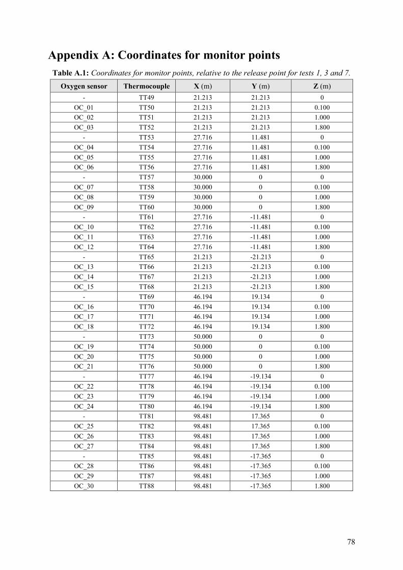
78

Appendix A: Coordinates for monitor points

Table A.1: Coordinates for monitor points, relative to the release point for tests 1, 3 and 7.

Oxygen sensor Thermocouple X (m) Y (m) Z (m)

- TT49 21.213 21.213 0

OC_01 TT50 21.213 21.213 0.100

OC_02 TT51 21.213 21.213 1.000

OC_03 TT52 21.213 21.213 1.800

- TT53 27.716 11.481 0

OC_04 TT54 27.716 11.481 0.100

OC_05 TT55 27.716 11.481 1.000

OC_06 TT56 27.716 11.481 1.800

- TT57 30.000 0 0

OC_07 TT58 30.000 0 0.100

OC_08 TT59 30.000 0 1.000

OC_09 TT60 30.000 0 1.800

- TT61 27.716 -11.481 0

OC_10 TT62 27.716 -11.481 0.100

OC_11 TT63 27.716 -11.481 1.000

OC_12 TT64 27.716 -11.481 1.800

- TT65 21.213 -21.213 0

OC_13 TT66 21.213 -21.213 0.100

OC_14 TT67 21.213 -21.213 1.000

OC_15 TT68 21.213 -21.213 1.800

- TT69 46.194 19.134 0

OC_16 TT70 46.194 19.134 0.100

OC_17 TT71 46.194 19.134 1.000

OC_18 TT72 46.194 19.134 1.800

- TT73 50.000 0 0

OC_19 TT74 50.000 0 0.100

OC_20 TT75 50.000 0 1.000

OC_21 TT76 50.000 0 1.800

- TT77 46.194 -19.134 0

OC_22 TT78 46.194 -19.134 0.100

OC_23 TT79 46.194 -19.134 1.000

OC_24 TT80 46.194 -19.134 1.800

- TT81 98.481 17.365 0

OC_25 TT82 98.481 17.365 0.100

OC_26 TT83 98.481 17.365 1.000

OC_27 TT84 98.481 17.365 1.800

- TT85 98.481 -17.365 0

OC_28 TT86 98.481 -17.365 0.100

OC_29 TT87 98.481 -17.365 1.000

OC_30 TT88 98.481 -17.365 1.800

79

Table A.2: Coordinates for monitor points, relative to the release point for Test 2.

Oxygen sensor Thermocouple X (m) Y (m) Z (m)

TT49 21.213 21.213 0

OC_01 TT50 21.213 21.213 0.100

OC_02 TT51 21.213 21.213 1.000

OC_03 TT52 21.213 21.213 1800

TT53 27.716 11.481 0

OC_04 TT54 27.716 11.481 0.100

OC_05 TT55 27.716 11.481 1.000

OC_06 TT56 27.716 11.481 1.800

TT57 30.000 0 0

OC_07 TT58 30.000 0 0.100

OC_08 TT59 30.000 0 1.000

OC_09 TT60 30.000 0 1.800

TT61 27.716 -11.481 0

OC_10 TT62 27.716 -11.481 0.100

OC_11 TT63 27.716 -11.481 1.000

OC_12 TT64 27.716 -11.481 1.800

TT65 21.213 -21.213 0

OC_13 TT66 21.213 -21.213 0.100

OC_14 TT67 21.213 -21.213 1.000

OC_15 TT68 21.213 -21.213 1.800

TT74 -27.716 11.481 0

OC_16 TT75 -27.716 11.481 0.100

OC_17 TT76 -27.716 11.481 1.000

OC_18 TT77 -27.716 11.481 1.800

TT78 -30.000 0 0

OC_19 TT79 -30.000 0 0.100

OC_20 TT80 -30.000 0 1.000

OC_21 TT81 -30.000 0 1.800

TT82 -27.716 -11.481 0

OC_22 TT83 -27.716 -11.481 0.100

OC_23 TT84 -27.716 -11.481 1.000

OC_24 TT85 -27.716 -11.481 1.800

TT86 0.800 0

OC_25 TT87 0.800 0.100

OC_26 TT88 0.800 1.000

OC_27 TT89 0.800 1.800

TT89 6.700 9.000 0

OC_28 TT90 6.700 9.000 0.100

OC_29 TT91 6.700 9.000 1.000

OC_30 TT92 6.700 9.000 1.800

80

Appendix B – Results from experiments and simulations

Table B.1: Comparison of temperatures and H2-Concentrations measured in Test 1, Test 3 -

Test7 with data from simulations.

Lowest

Temperature,

Radius 30 m

Lowest

Temperature,

Radius 50 m

and 100 m

Highest H2-

Concentration,

0.1 m high

Oxygen Sensor

Highest H2-

Concentration,

1.0 m high

Oxygen Sensor

Highest H2-

Concentration,

1.8 m high

Oxygen Sensor

Test 1

Experiment -2.9 C -0.5 C 0.9 vol% 1.8 vol% 1.5 vol%

FLACS -7 C -1.2 C 3.4 vol% 2.2 vol% 1.8 vol %

Test 3

Experiment -8 C -0.4 C 6.4 vol% 8.6 vol% 5.8 vol%

FLACS -17.2 C -2 C 8.7 vol% 6.9 vol% 4.9 vol %

Test 4

Experiment -26.8 C -10.9 C 17.2 vol% 16.8 vol% 11.9 vol%

FLACS -15 C -10.4 C 8.2 vol% 6.4 vol% 4.7 vol%

Test 5

Experiment -8.5 C -1.5 C 6.2 vol% 7.7 vol% 7.6 vol%

FLACS -17.3 C -4.8 C 8.8 vol% 7.5 vol% 7.2 vol%

Test 6

Experiment -25.7 C -2 C 22 vol% 31 vol% 22 vol%

FLACS -16 C -2.7 C 8 vol% 8 vol% 6.6 vol%

Test 7

Experiment -0.2 C 1.5 C 2.5 vol% 2.7 vol% 2.2 vol%

FLACS -2.6 C -1.0 C 2.5 vol% 1.7 vol% 1.1 vol%

Table B.2: Comparison of temperatures and H2-Concentrations measured in Test 2 with data

from simulations.

Lowest

Temp.,

Radius 30

m

(West)

Lowest

Temp.,

Radius 30

m

(East)

Lowest

Temp.,

Front of

ISO

container

Highest H2-

Concentration

, Radius 30m

(west)

Highest H2-

Concentration

, Radius 30m

(East)

Highest H2-

Concentration

, Front of ISO

container

Experiment -7.6 C 1 C 1 C 4.2 vol% 0 vol% 0 vol%

FLACS -20 C 1.2 C 1.4 C 9.4 vol% 0 vol% 0 vol%

Table B.3: Simulation results from varying Pasquill classes.

Pasquill Class A B C D E F

Highest

H2-concentration 17.7 vol% 14 vol% 14.1 vol% 11.3 vol% 10.2 vol% 8.8 vol%

Lowest temperature

-37.3 C -28.5 C -28.8 C -22.4 C -19.8 C -17.3 C

81

Table B.4: Simulation results from varying different wind velocities

Wind Velocity 0.5 m/s 1 m/s 5 m/s 10 m/s 15 m/s 20 m/s 25

m/s

30

m/s

Highest

H2-concentration

7.9

vol%

9

vol%

11

vol%

10

vol%

0.84

vol%

0.7

vol%

0.6

vol%

0.5

vol%

Lowest

temperature -15.5 C -17.9 C -22.6 C -20.3 C 0.97 C 1.3 C 1.5 C 1.7 C

Table B.5: Simulation results from varying grid cell size

Using data

form Test 4

Lowest

Temperature,

Radius 30 m

Lowest

Temperature,

Radius 50 m

and 100 m

Highest H2-

Concentration,

0.1 m high

Oxygen Sensor

Highest H2-

Concentration,

1.0 m high

Oxygen Sensor

Highest H2-

Concentration,

1.8 m high

Oxygen Sensor

Experiment -26.8 C -10.9 C 17.2 vol% 16.8 vol% 11.9 vol%

FLACS

Grid Cell Size

0.30 m -15 C -10.4 C 8.2 vol% 6.4 vol% 4.7 vol%

0.20 m -15.5 C -10.0 C 8.1 vol% 6.4 vol% 4.6 vol%

0.25 m -16.7 C -8.9 C 8.6 vol% 6.9 vol% 5.0 vol%

0.35 m -63.3 C -2.5 C 28.7 vol% 25.5 vol% 10.8 vol%

0.40 m -29.0 C -1.5 C 13.9 vol% 11.5 vol% 7.4 vol%

Table B.6: Simulation results from varying initial/outdoor temperature

Using data

form Test 4

Lowest

Temperature,

Radius 30 m

Lowest

Temperature,

Radius 50 m

and 100 m

Highest H2-

Concentration,

0.1 m high

Oxygen sensor

Highest H2-

Concentration,

1.0 m high

Oxygen sensor

Highest H2-

Concentration,

1.8 m high

Oxygen sensor

Experiment -26.8 C -10.9 C 17.2 vol% 16.8 vol% 11.9 vol%

FLACS,

Initial

temperature

3.3 C -15 C -10.4 C 8.2 vol% 6.4 vol% 4.7 vol%

10 C -11.6 C -4.5 C 9 vol% 7.5 vol% 5.7 vol%

20 C -3.3 C 4.48 C 9.38 vol% 7.8 vol% 5.8 vol%

30 C 6.7 C 13.78 C 9.03 vol% 7.15 vol% 5.17 vol%

-5 C -25.3 C 17 C 9.06vol% 7.5 vol% 5.5 vol%

-10 C -30.2 C -21.78 C 9.20 vol% 7.5vol% 5.5 vol%

-15 C -36 C -24.9 C 9.77 vol% 7.9 vol% 5.64 vol%

-20 C -39.1 C -29.2 C 9.11 vol% 7.2 vol% 5.1 vol%