towards a methodology doctoral dissertation study of the
TRANSCRIPT

DOCTORAL DISSERTATION Study of the frictional behaviour of planar saw-cut rock surfaces towards a methodology for tilt testing and its application to case studies ‘International Mention’ Ignacio Pérez Rey 2019
DO
CT
OR
AL
DIS
SER
TA
TIO
N S
tudy
of t
he fr
ictio
nal b
ehav
iour
of p
lana
r sa
w-c
ut r
ock
surf
aces
tow
ards
a m
etho
dolo
gy
for
tilt t
estin
g an
d its
app
licat
ion
to c
ase
stud
ies.
Ign
acio
Pér
ez R
ey, 2
019

International Doctoral School
Ignacio Pérez Rey
DOCTORAL DISSERTATION
Study of the frictional behaviour of planar saw-cut rock
surfaces towards a methodology for tilt testing and its
application to case studies
Supervised by: Leandro R. Alejano Monge, PhD
2019
‘International Mention’

International Doctoral School
Leandro R. Alejano Monge:
DECLARES that the present work, entitled ‘Study of the frictional behaviour of
planar saw-cut rock surfaces towards a methodology for tilt testing and its
application to case studies’, submitted by Ignacio Pérez Rey to obtain the title of
Doctor, was carried out under his supervision in the PhD programme
‘Mathematical Modelling and Numerical Simulation in Engineering and
Applied Science’. This is a joint PhD programme integrating the Universities of
Vigo, Santiago de Compostela and A Coruña.
Vigo, April 11th 2019

Acknowledgements
‘En luteam olim, celebra marmoream’
Francisco Jimenez de Cisneros, 1513
First of all, I would like to thank my thesis supervisor, Dr. Leandro R. AlejanoMonge, for accepting me as part of his research team as well as for being an excellentmentor, not only in the process of learning rock mechanics, but also in other equallyrelevant aspects in the development of a researcher. Leandro: thank you.
I would also like to thank all the researchers involved in the benchmark experimentand in the development of the Suggested Method. Without a doubt, an unprecedentedexperience, both from a scientific and human point of view.
The two research stays carried out in the National Laboratory for Civil Engineering(LNEC, Portugal) and in the Department of Civil Engineering (University of Alicante,Spain) allowed me to learn while discovering outstanding people. Special thanks tomy supervisor during my research stay at the LNEC, Dr. Jose Muralha, and to thepeople from the UA: Dr. Roberto Tomas, Dr. Adrian Riquelme and Dr. Miguel Cano.
Special thanks to Dr. Carmen Serra and her team (Paula Barbazan and TatianaPadın) for their accessibility and for all the knowledge and support transmitted whencarrying out the surface topography studies.
I have known Javier Martınez for more than 12 years. Without a doubt, specialthanks to you for being a sort of ‘big brother’, in every good way.
Finally, but not less importantly, I would like to mention all those colleagues who,in a more or less intimate way, were part of my time and life in the Department andwho undoubtedly contributed, one-by-one, to making my time in the ‘JPH’ laboratoryunforgettable.
The development of this thesis would not be possible without the financial supportprovided by the current Ministry of Economy and Business of the Spanish Government(Ministerio de Economıa y Empresa) through the contract BIA2014-53368P, partiallyfinanced by means of ERDF funds of the EU.
i

ii

Aos meus.
iii

iv

Abstract
Rock masses are typically formed by rocks and they include a number of discontinu-ities of geological origin that tend to govern their behaviour. Researchers started tounderstand this in parallel with the development of rock engineering. Accordingly, inthe 60’s and 70’s of the past century, the relevant mechanical role of these discontinu-ities was started to be treated in a more rigorous manner. This is why, at that time,together with other relevant advances, a rather accurate shear strength criterion forrock joints was proposed, crystallizing in the so-called Barton-Bandis approach.
This formulation is typically used to compute shear strength of rock discontinuitiesin practical rock engineering. It needs five input parameters, namely, basic frictionangle potentially derived from tilt tests, joint roughness coefficient, joint compres-sive strength (potentially derived from Schmidt hammer rebounds on the rock joint),Schmidt hammer rebounds on fresh rock and scale, and one variable, normal stress.From these inputs the basic friction angle is one that often has the largest impact onrock joint shear strength. However, the procedure to estimate it, typically based ontilt testing, has been poorly studied.
A large number of shear strength criteria for rock joints have been developed sofar. A relevant effort has been put on the estimation of roughness input parameters.However, the basic frictional component (typically the basic friction angle) has beenless studied, it can be said that it has been somehow disregarded. An incorrect esti-mation of this parameter can lead to a misinterpretation of the shear strength of rockdiscontinuities, with potentially significant impact on rock engineering design.
Based on the aforementioned reasons, this PhD thesis is intended to study in depthwhat is known as ‘basic friction angle’ of rock discontinuities, as well as the natureand influence of several experimental parameters (like time, wear, tilting rate, geome-try or micro-roughness) in relation to tilt-test results. Various experimental programsaddressing one or some of these parameters were carried out to quantify their impacton basic friction angle. Statistical tools were used to interpret dataset results. Ad-ditionally, in collaboration with other research institutions, an experimental programor benchmark study was carried out to check how different procedures followed indifferent laboratories might affect results.
v

vi
This multi-country experimental benchmark study demonstrated that sliding an-gles for saw-cut rock surfaces determined by tilt tests performed in different laborato-ries tend to be similar when test conditions are sufficiently controlled. Attention wasdrawn on surface wear, cutting procedures, test sliding distance, cleaning practicesand potential vibration produced by the tilting table as issues potentially affectingresults. Based on this study, it was considered appropriate to try to advance towardsstandardization of tilt tests by controlling the most important factors affecting results.
Relying on previous experimental based findings, this thesis is proposed as a sup-porting work for the development of a suggested methodology for tilt testing —ISRMSuggested Method, (Alejano et al., 2018a)—, conceived to provide a straightforwardprocedure to obtain sufficiently reproducible and reliable test results.
As a final phase and example of application of the developed studies, knowledgeacquired in relation to tilt testing and basic friction angle has been applied to thestudy of the stability of an irregular granite boulder. A stability assessment againstsliding and toppling of this paradigmatic ellipsoid-shaped granitic boulder, known asthe Pena do Equilibrio and located in Ponteareas (Pontevedra, Spain) was carried out.For this study, other innovative techniques, such as photogrammetry from UnmannedAerial Vehicle (UAV) and terrestrial laser scanner (LiDAR) were applied for an ac-curate computation of the boulder geometry. In turn, this opened the door for moreaccurate stability assessment of complex-geometry boulders and other rock structures,something that was difficult to carry out in the past due to the difficulties in computingodd-shape boulder geometry.

Resumen
Las rocas se presentan en la corteza terrestre en forma de macizos rocosos. Un macizorocoso esta compuesto de roca, que a su vez presenta discontinuidades o juntas deorigen geologico diverso, las cuales tienden a regir su comportamiento. Este hecho secomenzo a comprender y a tener en cuenta en el ambito de la investigacion a medidaque fue evolucionando la ingenierıa de los macizos rocosos. En los anos 60 y 70 delsiglo pasado, se comenzo a tratar de una manera mas rigurosa el papel que jueganestas discontinuidades en el comportamiento mecanico de los macizos rocosos. Esta esla razon por la que, en aquel momento, junto con otros avances relevantes, se propusoun criterio relativamente preciso para la determinacion de la resistencia al corte de lasjuntas en roca, que cristalizarıa anos despues en lo que hoy se conoce como el enfoquede Barton-Bandis.
Esta formulacion propuesta por Barton y Bandis (1982), se utiliza en ingenierıaaplicada para calcular la resistencia al corte de las discontinuidades de roca. Necesitacinco parametros de entrada, a saber, el angulo de friccion basico, potentcialmentederivado del ensayo de inclinacion o tilt-test, el coeficiente de rugosidad de la junta,la resistencia a la compresion de la junta (potencialmente derivada del numero derebotes del martillo Schmidt o esclerometro en la junta de la roca), el numero derebotes del martillo Schmidt en roca fresca y la escala, ademas de una variable, latension normal a la que esta sometida la junta. De estos parametros, el angulo defriccion basico es el que a menudo tiene el mayor impacto en la resistencia al corte dela discontinuidad. Sin embargo, el procedimiento para estimarlo, tıpicamente basadoen ensayos de inclinacion o tilt tests, no ha sido estudiado con demasiada profundidad.
Hasta la fecha se han propuesto un buen numero de criterios de resistencia al cortede juntas o discontinuidades en roca. Los estudios en este ambito parecen habersecentrado mas en la estimacion de los parametros de entrada geometricos, como larugosidad, que en otros aspectos. Sin embargo, el componente de friccion basica(tıpicamente denominado angulo de friccion basico) ha sido en general menos estu-diado, teniendose apenas en cuenta en algunos casos. Sin embargo, una estimacionincorrecta de este parametro puede llevar a una mala interpretacion de la resistenciaal corte de las discontinuidades de roca, con un impacto potencialmente significativoen los disenos y analisis de estabilidad en la realizacion de obras a cielo abierto ysubterraneas.
vii

viii
Por las razones antes mencionadas, esta tesis de doctorado estudia en profundidadel denominado angulo de friccion basico de las discontinuidades en roca, ası como lanaturaleza y la influencia de varios parametros experimentales (como el tiempo, el des-gaste, la velocidad de inclinacion, la geometrıa de las probetas o la micro-rugosidad) enrelacion a los resultados de los ensayos tipo tilt test utilizados para su cuantificacion.Para ello, se llevaron a cabo varios programas experimentales que abordan uno o variosde estos parametros para cuantificar su impacto en la medida del angulo de friccionbasico. Se utilizaron tambien tecnicas estadısticas para interpretar los resultados delos conjuntos de datos obtenidos. Ademas, en colaboracion con otros organismos yuniversidades, se llevo a cabo un programa experimental (considerado como un estudiode referencia, o benchmark) para analizar como los diferentes procedimientos seguidosen diferentes laboratorios afectan a los resultados.
Entre los antedichos factores, se presto atencion al desgaste de la superficie, a losprocedimientos de corte, a la longitud de deslizamiento de la probeta, al procedimientode limpieza de la superficie y a la potencial vibracion producida por la maquina de en-sayos, ya que estos podrıan tener influencia sobre los resultados. Este estudio compar-ativo experimental internacional demostro que los angulos de deslizamiento o friccionbasica obtenidos mediante ensayos de inclinacion en superficies de rocas serradas, tien-den a ser similares cuando las condiciones de ensayo estan suficientemente controladas.A partir del analisis de los resultados de todos estos estudios, se considero apropiadointentar avanzar hacia la estandarizacion del ensayo de inclinacion o tilt test medianteel control de los factores experimentales mas importantes que afectan los resultados.Basandose en lo aprendido en dichos estudios, esta tesis se propuso como un trabajode apoyo para el desarrollo de una metodologıa sugerida (Suggested Method, denom-inacion establecida por la Sociedad Internacional de Mecanica de Rocas e Ingenierıade Rocas o ISRM) para la obtencion del angulo de friccion basico de discontinuidadesen roca mediante ensayos de inclinacion o tilt tests, concebida para proporcionar unprocedimiento sencillo, regulado y reproducible para obtener este parametro tan rele-vante. Este metodo sugerido, aceptado como norma en muchos paıses, fue publicadoa finales del ano pasado (Alejano et al., 2018a).
Como fase final y ejemplo de aplicacion de los estudios desarrollados, el conocimientoadquirido en relacion a los ensayos de inclinacion y la obtencion del angulo de friccionbasica, se han aplicado al estudio y evaluacion de la estabilidad frente al deslizamientoy al vuelco de un bolo granıtico paradigmatico, conocido como la Pena do Equilibrioy localizado en el ayuntamiento de Ponteareas (Pontevedra). Para este estudio se hanaplicado otras tecnicas novedosas como la fotogrametrıa desde dron y laser escanerterrestre para definir su geometrıa. La combinacion de tecnicas de caracterizaciongeomecanica rigurosas, como las propuestas en el seno de esta tesis, con tecnicas to-pograficas avanzadas han permitido realizar un estudio riguroso de la estabilidad dedicho bolo, lo que representa un avance de interes en el ambito de la mecanica derocas.

Extended abstract
Rock masses are typically formed by rocks and they include a number of discontinu-ities of geological origin that tend to govern their behaviour. Researchers started tounderstand this in parallel with the development of rock engineering. Accordingly, inthe 60’s and 70’s of the past century, the relevant mechanical role of these discontinu-ities was started to be treated in a more rigorous manner. This is why, at that time,together with other relevant advances, a rather accurate shear strength criterion forrock joints was proposed, crystallizing in the so-called Barton-Bandis approach.
This formulation is typically used to compute shear strength of rock discontinu-ities in practical rock engineering. It needs five input parameters, namely basic frictionangle derived from tilt test, joint roughness coefficient, joint compressive strength (po-tentially derived from Schmidt hammer rebound on the rock joint), Schmidt hammerrebound on fresh rock, scale; and one variable, normal stress. From these inputs thebasic friction angle is one that often has the largest impact on rock strength. However,the procedure to estimate it, typically based on tilt testing, has been poorly studied.
A large number of shear strength criteria for rock joints have been developed sofar. A relevant effort has been put on the estimation of roughness input-parameters.However, the basic frictional component (typically the basic friction angle) has beenless studied, it can be said that it has been somehow disregarded. An incorrect esti-mation of this parameter can lead to a misinterpretation of the shear strength of rockdiscontinuities, with potentially significant impact on rock engineering design.
Despite having devoted relatively great attention to the characterization of thegeometric properties of the joints (as, for example, roughness or anisotropy), most ofthe criteria for estimating rock joint shear strength developed to date have paid lessattention to the determination of the basic frictional component, typically identifiedas the basic friction angle. This fact may also be motivated by the lack of an adequatemethodology on which the estimation of this parameter could be based.
Problems in obtaining and using the basic friction angle have been detected, forexample, in some case studies applied to real mining operations (Wines and Lilly,2003; Alejano et al., 2012a) as well as in other practical works focusing the study ofcomplex mechanism slope stability cases (Alejano et al., 2019).
ix

x
That is why this PhD thesis focuses to study in depth what is known as the basicfriction angle of rock discontinuities. In addition, it is proposed to develop a suggestedmethodology for its estimation. This will be based on experimental and statisticalstudies, as well as in the performance of various experiments in collaboration with dif-ferent researchers belonging to other rock mechanics laboratories in several countries.Finally, the results and the methodology suggested in this work, together with otherad-hoc studies, is applied to the study of a real case, consisting of the stability analysisof an irregular granite boulder.
In the first part of this thesis (Chapter 1), the problem to be studied is contextu-alized in the field of rock mechanics and rock mass engineering. The main objectivesof the work are presented. Also included here is a review of the publications derivedtotally or partially from this thesis work, published both in international congressesand in JCR-indexed journals.
In Chapter 2, a general overview on shear strength of rock joints is presented. Inthis state of the art, the mechanical properties of the discontinuities are introduced.This includes the cohesion and existence of rock bridges, the roughness at differentscales and, fundamentally, the basic friction, the parameter object of study in thiswork. Then, a revision of the rock joint shear strength criteria is presented. From thisreview, it is evident that the different empirically-based available criteria are advancedversions of the equation proposed by Mohr-Coulomb, in which shear strength presentsa basic frictional component (mobilized by the normal tension applied) together witha cohesive component.
The determination of this basic friction angle has traditionally been carried outby means of three types of tests. Firstly, by means of direct shear tests in flat joints.Secondly, by means of pull-test or push-test, which represent simpler versions of thedirect shear test, where the load is transmitted in a less sophisticated way (potentiallyby means of a dead weight, such as a container with sand). Ultimately, the basicfriction angle can be computed by means of tilt-tests, through the use of differenttypes of blocks (prismatic or cylindrical, from rock drill core). While the techniquedescribed as a direct shear tests initially require an industrious preparation of the testspecimens; pull- and push-tests require some interpretation of the applied stresses inorder to estimate the friction angle.
Tilt-tests consist, basically, in making a block sliding on a contact. This techniqueis based on the concept of angle of repose, characteristic of granular materials, as wellas the classic problem of a block located on an inclined plane. The technique describedhas its origins, in the field of rock mechanics, in the studies carried out to estimatethe friction between mineral particles (Horn and Deere, 1962) and sedimentary rocks(Ripley and Lee, 1962). Seminally proposed by Hoek and Bray (1974), later on, sev-eral authors deepened in the study of frictional behaviour, developing some models ofprimitive tilting tables, such the case of Cawsey and Farrar (1976).

xi
Other authors, such as Hencher (1976, 1977), devoted relatively extensive effortsto the analysis of the slip angle obtained from saw-cut planar rock joints, also account-ing for the role of vibration. This author also introduced the study of wear, a factorthat is particularly relevant when interpreting the results of series of several tests.Undoubtedly, the introduction of the Barton-Bandis approach (Barton and Bandis,1982), raised the need for a correct estimation of the basic friction angle. For ex-ample, Barton and Choubey (1977) present a motorized table for the performance ofinclination or tilt tests.
An important advance or, at least, one more step in the estimation of the basicfriction angle of the discontinuities is given in 1981 by Stimpson (1981), who proposesthe use of cylindrical rock cores to estimate the mentioned parameter. This wouldbe done by placing a rock core on two others, in contact along their generatrixes.Although this author proposed a formulation to obtain the basic friction angle, overthe years an error in the formula would be detected. Stimpson’s proposal (Stimpson,1981) opened the door to rock core testing, which allowed an improvement, in practicalterms, for the estimation of the basic friction angle in the field. Also, using drill coresamples, years later Barton (2011) proposed the use of only two cores to obtain thebasic friction angle. The novelty of this proposal was that it avoided the wedging ofthe cores, which allowed obtaining non-overestimated results.
In recent years, several authors, including some from the University of Vigo (Ale-jano et al., 2012a; Gonzalez et al., 2014; Ruiz and Li, 2014; Perez-Rey et al., 2016;Ulusay and Karakul, 2016; Li et al., 2017; Jang et al., 2018) have made efforts toimprove the tilting machines and available procedures. However, there were still cer-tain aspects deserving further attention. The present doctoral thesis addresses theseaspects, based on the experimental and statistical study of the influence of variousfactors on the results and with the objective to develop a suggested methodology—ISRM Suggested Method, (Alejano et al., 2018a)—for the estimation of the basicfriction angle.
Chapter 3 analyses the influence of several experimental factors on tilt testing andit is the core of this work. This includes those experimental factors inherent in theperformance of an inclination test, from the nature of the rock to the realization ofthe test itself. More than 2,000 tests are behind the presented results and analyses.In this experimental section, a detailed study of each parameter was developed, inwhich it has been observed that geometry, wear and roughness are relevant factorswhen evaluating the results of inclination tests. The speed of the tilt table, within theranges studied in this work, does not seem to affect the results in a relevant way.
This set of experimental studies showed that the sliding angles obtained by incli-nation tests on saw-cut surfaces and tested at different laboratories, tend to be similarwhen the test conditions are sufficiently controlled. Among the factors mentioned,special attention was paid to the wear of the surface, the cutting procedures, thesliding path of the specimen, the cleaning procedure of the surface and the potentialvibration produced by the test machine.

xii
All these factors have shown to affect results. Based on observations, it was consid-ered appropriate to proceed towards the standardization of the tilt test by controllingthe most relevant experimental factors affecting the testing process and, consequently,the results.
These experimental results were also analysed from a statistical perspective, some-thing illustrated in Chapter 4. Here, the statistical analyses, both descriptive andinferential, of those results from the reference study carried out with rock mechan-ics laboratories from different countries, are shown. Then, a statistical study basedon a program that included the performance of more than 250 tests with specimensthat presented various combinations of experimental parameters such as the length-to-thickness ratio, the lifting velocity of the tilting table or the type of cutting sawwas also presented (Perez-Rey et al., 2018).
Once all this information was collected and some relevant conclusions derived; theauthor of this research work actively participated as a member of the Working Groupinvolved in the drafting of an ISRM Suggested Method for the determination of thebasic friction angle by means of tilt test. This ISRM SM was eventually approvedby the International Society of Rocks Mechanics and Rock Engineering (ISRM) andpublished in the journal Rock Mechanics and Rock Engineering (Alejano et al., 2018a).
As a final phase of the thesis, the stability analysis of a singular geological struc-ture was proposed in Chapter 6 of this thesis. This referred to a granitic boulder inthe province of Pontevedra (Galicia, Spain), which is known as Pena do Equilibrio.This irregular granite element consists of a sub-ellipsoidal shaped and roughly 400 tboulder located on a mountain slope. The main characteristic that has motivated hisstudy is the sensation of instability, according to his name (‘Balanced Stone’) that itcauses to the observer.
The first step for the study of this structure consisted of a program of laboratorytests. First, we review the equations classically proposed for the calculation of blocktoppling and adapt them to irregular rock blocks. Then, we evaluated the effect of acurved contact on the stability of specimens. In addition, the effect produced by thelocation of the center of gravity of an element outside the planes of symmetry has beenstudied, an aspect that is especially relevant when studying the stability of irregularboulders. For this purpose, rock and steel specimens were used, which, subjected totilt tests, allowed to check the analytical formulations specifically developed for thecalculation of the safety coefficient of this rock in relation to toppling and sliding fail-ure mechanisms.
Another uneasy task was the estimate of the boulder weight and shape. This hasbeen possible thanks to the successful application of advanced topographic techniques,such as the Terrestrial Laser Scanner (LiDAR) and aerial photogrammetry throughthe use of a drone. The first technique allowed a very detailed description of the area ofcontact between the boulder and the rock mass, and the second permitted computing

xiii
the volume of the boulder and the position of its gravity center in an accurate manner.Indeed, with the topographical information collected, a 3D point cloud was generatedwhich, with subsequent treatment, allowed obtaining the mentioned geometrical as-pects extremely relevant when computing stability of the block.
As a result of this study, the factors of safety against sliding (FS = 1.31) andagainst toppling (FS = 1.20) were determined. In addition, these FS were calculatedin the event of an earthquake, both for the case contemplated in the Spanish buildingregulations (MFOM, 2002) that return results for sliding and toppling of 1.20 and 1.11respectively; as well as for the occurrence of an extraordinary earthquake, which wouldreduce the FS to values at which the stability of the boulder would be compromised.In addition, a scale model of the stone was made by means of 3D printing on PLAplastic, which allowed the realization of several tilt tests representing actual behaviorand providing sliding angles similar as those analytically computed. This opens adoor to the realization of laboratory tests with physical models, a novel methodologyand of great interest when studying phenomena associated with elements of complexgeometry in the field of rock mass engineering.
All in all, in this thesis some steps forward have been done towards a better un-derstanding of the shear strength of rock contact surfaces. A better knowledge of thefactors affecting tilt tests was achieved. This has served to the proposal of a suggestedmethod for obtaining the basic friction angle of planar rock surfaces by means of tilttests. Additionally, tilt tests have shown to be an interesting methodology for betterunderstand and compute the stability of irregular rock boulders in natural slopes.

xiv

Resumen extendido
Los macizos rocosos estan tıpicamente formados por rocas incluyendo tambien unaserie de discontinuidades de origen geologico, las cuales tienden a regir su compor-tamiento. Estas discontinuidades afectan al macizo rocoso a distintos niveles, desdeuna escala kilometrica (como es el caso de las fallas), a una escala de centenas o dece-nas de metros (como es el caso de las juntas) e incluso en el seno de lo que se denomina‘roca intacta’ (como en el caso de las fisuras o defectos).
Esta particularidad natural de los macizos rocosos, se comenzo a comprender y atener en cuenta en el ambito de la investigacion a medida que fue evolucionando la in-genierıa de los macizos rocosos. En consecuencia, en los anos 60 y 70 del siglo pasado,se comenzo a tratar de una manera mas rigurosa el papel, fundamentalmente mecanico,jugado por estas discontinuidades. Esta es la razon por la que, en aquel momento,junto con otros avances relevantes, se propuso un criterio bastante preciso, a la vez quesuficientemente sencillo, para la determinacion de la resistencia al corte de las juntasde roca, cristalizado en lo que se conoce como el enfoque Barton-Bandis en el ano 1982.
Esta formulacion propuesta por Barton y sus colaboradores se utiliza normalmentede manera eminentemente practica, para calcular la resistencia al corte de las discon-tinuidades de roca. Necesita cinco parametros de entrada, concretamente, el angulode friccion basico (potencialmente derivado del ensayo de inclinacion o tilt-test), el co-eficiente de rugosidad de la junta JCR, la resistencia a la compresion de la junta, JCS(potencialmente derivada del numero de rebotes del martillo Schmidt o esclerometroen la junta de la roca r), el numero de rebotes del martillo Schmidt en roca fresca (R)y la escala, ademas de una variable, la tension normal a la que esta sometida la junta.De estos parametros de entrada, el angulo de friccion basico es el que a menudo tieneel mayor impacto en la resistencia cortante o de cizalla de la discontinuidad. Sin em-bargo, el procedimiento para estimarlo, tıpicamente basado en ensayos de inclinacion,ha sido poco estudiado y escasamente descrito.
Este hecho se observa tambien en la mayorıa de los criterios para la estimacion de laresistencia al corte de las discontinuidades desarrollados hasta la fecha, analizados enun estudio publicado por Singh and Basu (2018), en los cuales, a pesar de haber ded-icado relativamente gran atencion a la caracterizacion de las propiedades geometricasde las juntas (como, por ejemplo, la rugosidad o la anisotropıa), se ha prestado menosatencion a la determinacion de la componente friccional basica, tıpicamente identi-
xv

xvi
ficada como el angulo de friccion basico. Este hecho puede venir motivado tambienpor la carencia de una metodologıa adecuada sobre la que basar la estimacion de esteparametro.
Es relevante destacar que una estimacion incorrecta de la componente friccionalbasica puede llevar a una mala interpretacion de la resistencia al corte de las dis-continuidades de roca, con un impacto potencialmente significativo en el diseno yejecucion de obras a cielo abierto (como taludes para la ingenierıa minera y civil ocortas mineras) ası como en el desarrollo de obras subterraneas (tuneles, minas pro-fundas, explotacion de yacimientos de gas y petroleo).
Problemas en la obtencion y utilizacion del angulo de friccion basica se han puestode manifiesto, por ejemplo, en algun caso de estudio aplicado a explotaciones minerasreales, desarrollados hasta la fecha por algunos investigadores (Wines and Lilly, 2003;Alejano et al., 2012a) ası como en otros trabajos de laboratorio dedicados al estudiodel mecanismo de vuelco mediante modelos fısicos, de los que el autor de la presentetesis de doctorado ha formado parte (Alejano et al., 2019).
Es por ello que esta tesis de doctorado esta destinada a estudiar en profundidadlo que se conoce como angulo de friccion basico de las discontinuidades de la roca.Se propone el desarrollo de una metodologıa sugerida para su estimacion basada enestudios experimentales y estadısticos, ası como en la realizacion de diversos experi-mentos en colaboracion con distintos investigadores pertenecientes a otros laboratoriosde mecanica de rocas de varios paıses. Finalmente, los resultados y la metodologıasugerida en el seno de este trabajo, junto con otros estudios ad-hoc, se aplica al estudiode un caso real, consistente en el analisis de estabilidad de un bolo granıtico irregularde origen natural, tanto frente a un mecanismo de deslizamiento como de vuelco.
En la primera parte de esta tesis (Capıtulo 1), se contextualiza en el ambito de lamecanica de rocas y de la ingenierıa de los macizos rocosos el problema a estudiar. Seplantean tambien los objetivos principales del trabajo. Se incluye ademas aquı unaresena de las publicaciones derivadas total o parcialmente de este trabajo de tesis,publicadas tanto en congresos internacionales como en revistas indexadas mediante elındice JCR.
En la segunda parte de la tesis, correspondiente al Capıtulo 2, se presenta primerouna vision general en referencia a resistencia al corte de las discontinuidades. En este‘estado del arte’, se realiza tambien una descripcion de las propiedades mecanicas de lasdiscontinuidades, las cuales dependen fundamentalmente de la cohesion y existenciade puentes de roca sana, la rugosidad a diferentes escalas y, fundamentalmente, dela friccion basica, el parametro objeto de estudio en este trabajo. A continuacion,se realiza una revision de los criterios de resistencia al corte de discontinuidades. Apartir de esta revision, es evidente la observacion de que los criterios basados enestudios empıricos no son mas que versiones avanzadas de la ecuacion propuesta porMohr-Coulomb, en la que la resistencia al corte presenta una componente friccionalbasica movilizada por la tension normal aplicada junto con una componente cohesiva.

xvii
El estudio de los criterios de resistencia al corte o cizalla de discontinuidades re-sulta una base fundamental para entender la necesidad de una correcta estimacion dela componente friccional basica (o angulo de friccion basico). Esto se puede compro-bar al observar que todas las ecuaciones presentadas hasta la fecha para estimar dicharesistencia dependen, ademas de la rugosidad y de otras caracterısticas mecanicas dela junta, de la componente friccional basica o, tıpicamente, del denominado angulo defriccion basico.
La determinacion de este angulo de friccion basico se ha venido realizando o bien atraves de ensayos de corte directo (o direct shear test) en juntas planas, o bien medi-ante ensayos tipo pull-test o push-test, los cuales representan versiones mas sencillasque el primero en los que la carga se transmite de una manera menos sofisticada (po-tencialmente mediante un peso muerto, como puede ser un recipiente con arena), perotambien tıpicamente a traves de ensayos de inclinacion o tilt-tests, mediante el uso dediferentes tipos de bloques (prismaticos o cilındricos, provenientes de testigos de rocade sondeos). Mientras que las tecnicas descritas como ensayo de corte directo inicial-mente requieren de una laboriosa preparacion de las probetas de ensayo; los pull- ypush- tests requieren de cierta interpretacion sobre las tensiones aplicadas para poderestimar el angulo de friccion, aunque se pueden considerar, en cierta manera, comouna alternativa practica sencilla de los ensayos de corte directo.
Los ensayos de inclinacion o tilt-tests consisten, basicamente, en hacer deslizar unbloque o probeta que, en contacto con otro bloque o probeta de la misma roca a lolargo de una superficie, se inclinan conjuntamente y de manera paulatina hasta queel bloque superior inicia su movimiento. Esta tecnica se fundamenta en el conceptode angulo de reposo, caracterıstico de los materiales granulares, ası como al clasicoproblema de un bloque situado en un plano inclinado.
La tecnica descrita tiene sus orıgenes, en el ambito de la mecanica de rocas, en losestudios realizados para la estimacion de la friccion entre partıculas minerales (Hornand Deere, 1962) y rocas sedimentarias (Ripley and Lee, 1962). Las primeras propues-tas para la estimacion del angulo de friccion basico mediante el ensayo de inclinacionvienen dadas por Hoek and Bray (1974). Posteriormente, varios autores profundizaronen el estudio del comportamiento friccional, desarrollando incluso para sus estudiosalgunos de los modelos de mesas de inclinacion primitivos (Cawsey and Farrar, 1976).
Otros autores, como Hencher (1976, 1977), dedicaron relativamente amplios esfuer-zos al analisis del angulo de deslizamiento obtenido a partir de juntas de roca planasy serradas, incluso teniendo en cuenta el efecto de las vibraciones y su influencia enlos resultados. Ademas, este ultimo autor introduce el papel del efecto del degaste,factor este particularmente relevante a la hora de interpretar los resultados de seriesde varios ensayos. Sin duda, la introduccion de los criterios de rotura para la resisten-cia al corte de las discontinuidades propuestos a finales de los anos 70 y a principiosde los anos 80, como es el caso de la formulacion de Barton (1977) o la llegada delcriterio de Barton-Bandis (Barton and Bandis, 1982), suscitan tambien la necesidadde una correcta estimacion del angulo de friccion basico. Ası, por ejemplo, Barton and

xviii
Choubey (1977) presentan una mesa motorizada para la realizacion de los ensayos deinclinacion o tilt-test.
Un avance importante o, al menos, un paso mas en la estimacion del angulo defriccion basico de las discontinuidades es dado en el ano 1981 por Stimpson (1981), elcual propone la utilizacion de testigos cilındricos de roca provenientes de sondeos paraestimar dicho parametro. Esto se realizarıa colocando un testigo sobre otros dos, encontacto a lo largo de sus generatrices. Sin embargo, con los anos se detectarıa un er-ror en la formula. La propuesta de Stimpson (1981) abrıa la puerta a realizar ensayoscon testigos, lo cual permitio una mejora, en terminos practicos, para la estimaciondel angulo de friccion basico en campo. Tambien empleando testigos de sondeos, anosdespues (Barton, 2011) propondrıa el uso de dos testigos en vez de tres para obtener elangulo de friccion basico. La novedad de esta propuesta es que evitaba el acunamientodel testigo superior, con lo cual permitıa obtener resultados en los que no se producıauna sobreestimacion asociada a este efecto de acunamiento.
En los ultimos anos, varios autores, y entre ellos algunos de la Universidad de Vigo(Alejano et al., 2012a; Gonzalez et al., 2014; Ruiz and Li, 2014; Perez-Rey et al., 2016;Ulusay and Karakul, 2016; Li et al., 2017; Jang et al., 2018) han realizado esfuerzosen mejorar las maquinas de inclinacion ası como los procedimientos para la realizacionde ensayos y la estimacion del angulo de friccion basico. Sin embargo, aun quedabanciertos aspectos que merecıan ser estudiados en mayor detalle, de ahı que se plantearala presente tesis doctoral, fundamentada en el estudio experimental y estadıstico de lainfluencia de diversos factores en los resultados de los ensayos de inclinacion y con elobjetivo de desarrollar una metodologıa sugerida —ISRM Suggested Method, (Alejanoet al., 2018a)—para la estimacion del angulo de friccion basico.
La influencia de varios factores experimentales se ha estudiado en el seno de estatesis, y el Capıtulo 3 supone el nucleo fundamental de este trabajo. Aquı, se hananalizado primeramente aquellos factores experimentales inherentes a la realizacionde un ensayo de inclinacion, desde la naturaleza de la roca hasta la realizacion delensayo en sı. Esto se ha llevado a cabo a partir de la realizacion de mas de 2.000ensayos. En este apartado experimental se desarrollado un estudio pormenorizado decada parametro, en el cual se ha podido observar que la geometrıa, el desgaste y larugosidad son factores relevantes a la hora de evaluar los resultados de los ensayos deinclinacion. La velocidad de la mesa de inclinacion, dentro de los rangos estudiadosen este trabajo, parece no afectar de manera relevante a los resultados de los ensayos.
En colaboracion con Grupo de Nanotecnologıa y Analisis de Superficies del Centrode Apoyo Cientıfico a la Investigacion (CACTI) (organismo perteneciente a la Uni-versidad de Vigo) se realizaron estudios de la rugosidad de las superficies de rocaserradas, empleadas en los ensayos de inclinacion. Si bien se han encontrado ciertascorrelaciones entre el comportamiento friccional y los parametros caracterısticos de larugosidad de las superficies ensayadas, se piensa que un estudio mas pormenorizado sehace necesario a la hora de entender mejor el comportamiento tribologico de este tipode contactos. Se ha podido observar tambien que parametros como la distribucion de

xix
picos y valles condicionan mas el comportamiento tribologico de las superficies. Sinembargo debido a que el ensayo presenta una fuerte componente direccional en cuantoal deslizamiento de la probeta, se plantea el estudio de parametros caracterısticos de latopografıa superficial de tipo direccional, como puede ser la derivada de la rugosidadmedia.
De manera paralela al estudio de los parametros experimentales que afectan a losensayos de inclinacion, el autor de esta tesis ha participado en la realizacion de unexperimento de referencia (benchmark) llevado a cabo entre varios investigadores elambito de la mecanica de rocas. Este estudio (Alejano et al., 2017), que involucroa universidades y organismos de Portugal, Turquıa y Noruega, sirvio, conjuntamentecon el trabajo de laboratorio realizado en la Universidad de Vigo, para determinar queel ensayo de inclinacion es reproducible y apropiado para la obtencion del angulo defriccion basico de las discontinuidades.
Este conjunto de estudios experimentales, demostro que los angulos de desliza-miento obtenidos mediante ensayos de inclinacion en superficies de rocas serradas yrealizados en diferentes laboratorios, tienden a ser similares cuando las condicionesde ensayo estan suficientemente controladas. Entre los antedichos factores, se prestoespecial atencion al desgaste de la superficie, a los procedimientos de corte, al recor-rido de deslizamiento de la probeta, al procedimiento de limpieza de la superficie y ala potencial vibracion producida por maquina de ensayos, ya que estos podrıan tenerinfluencia sobre los resultados. A partir de la base establecida mediante este estudio,se considero apropiado intentar avanzar hacia la estandarizacion del ensayo de incli-nacion mediante el control de los factores experimentales mas importantes que afectanal proceso de ensayo y, consecuentemente, a los resultados.
Los resultados de estos estudios experimentales se analizaron tambien de una man-era estadıstica, y se presentan en el Capıtulo 4 de esta tesis. Aquı, se muestran primerolos analisis estadısticos, tanto descriptivos como inferenciales de aquellos resultadosprovenientes del estudio de referencia llevado a cabo con laboratorios de mecanica derocas de distintos paıses. A continuacion, se presento tambien un estudio estadısticobasado en un programa que abarco la realizacion de mas de 250 ensayos con probetasque presentaban diversas combinaciones de parametros experimentales como son larelacion longitud/espesor, la velocidad de ensayo o el tipo de sierra de corte (Perez-Rey et al., 2018).
Una vez recopilada toda esta informacion ası como unas conclusiones claras, elautor de este trabajo de investigacion participo activamente como miembro del grupode trabajo (Working Group) dirigido por el director de esta tesis, y que se ocupo de lacreacion y redaccion de una metodologıa sugerida para la determinacion del angulo defriccion basico mediante el ensayo de inclinacion, aprobada por la Sociedad Interna-cional de Mecanica de Rocas e Ingenierıa de Rocas (ISRM) y publicada en la revistaRock Mechanics and Rock Engineering (Alejano et al., 2018a).
Como fase final de la tesis, se planteo el estudio de una estructura geologica sin-

xx
gular, como lo es un bolo granıtico situado en la provincia de Pontevedra (Galicia,Espana), que se conoce como Pena do Equilibrio. Este estudio se presenta en elcapıtulo 6 de esta tesis. Este elemento granıtico irregular consiste en un bolo de rocade forma sub-elipsoidal, localizado en una ladera de una montana. La caracterısticaprincipal que ha motivado su estudio es la sensacion de inestabilidad, de acuerdo a sunombre (‘Piedra del Equilibrio’) que provoca al ser observada.
El primer paso para el estudio de esta estructura consistio en un amplio pro-grama de ensayos en laboratorio, primeramente para revisar las ecuaciones propuestasclasicamente para el calculo de vuelco de bloques, ası como para evaluar el efecto deun contacto curvo en la estabilidad de probetas con forma de disco (tipo las empleadaspara los ensayos de traccion indirecta o brasilenos). Ademas se ha estudiado el efectoque produce la localizacion del centro de gravedad de un elemento fuera de los planosde simetrıa, un aspecto especialmente relevante a la hora de estudiar la estabilidad delbolo en cuestion. Para ello, se emplearon probetas de roca y acero que, sometidas aensayos de inclinacion o ‘tilt test’, permitieron comprobar las formulaciones analıticasespecıficamente desarrolladas para el calculo del coeficiente de seguridad de este boloen relacion a los mecanismos de estabilidad frente a vuelco y frente a deslizamiento.
Una vez testadas las ecuaciones del calculo del factor de seguridad, se procedio aestimar el volumen del bolo in situ. Esto ha sido posible gracias a la aplicacion exitosade tecnicas topograficas avanzadas, como son el Laser Escaner Terrestre (LiDAR) y lafotogrametrıa aerea mediante el empleo de un dron. La primera tecnica permitio unadescripcion muy detallada de la zona del contacto entre el bolo y el macizo rocoso, yla segunda una vision general del mismo ası como informacion de partes no accesiblesdesde el suelo, como la zona superior de la estructura geologica.
Recopilada esta informacion, se genero una nube de puntos 3D que, con un poste-rior tratamiento, permitio obtener el volumen del bolo ası como el area de contacto,aspectos estos muy relevantes a la hora de calcular las tensiones en la junta donde seestablece el contacto entre la roca y el macizo rocoso donde reposa.
Fruto de este estudio, se determinaron los coeficientes de seguridad frente a desliza-miento (FS = 1.31) y frente a vuelco (FS =1.20). Ademas, se calcularon estos coe-ficientes de seguridad en el caso de ocurrencia de un sismo, tanto para el caso con-templado en la normativa espanola (MFOM, 2002) que devuelven resultados paradeslizamiento y vuelco de 1.20 y 1.11 respectivamente; ası como para la ocurrencia deun sismo extraordinario, el cual reducirıa el coeficiente de seguridad hasta un valor enel cual la estabilidad del bolo se verıa comprometida.
Ademas, de manera complementaria, se realizo un modelo a escala del bolo medi-ante impresion 3D en plastico PLA, el cual permitio la realizacion de varios ensayos deinclinacion en los cuales se pudo observar cierto paralelismo entre los resultados de es-tabilidad obtenidos para la estructura real como para la replica. Esto abre una puertaa la realizacion de ensayos en laboratorio con modelos fısicos, metodologıa novedosay de gran interes a la hora de estudiar fenomenos asociados a elementos de geometrıa

xxi
compleja en el ambito de la ingenierıa de los macizos rocosos.
En general, en esta tesis, se han dado algunos pasos hacia una mejor comprensionde la resistencia al corte de las superficies de contacto de muestras de roca. Se halogrado un mejor conocimiento de la influencia de los factores que afectan los ensayostipo tilt test. Esto ha servido para proponer un metodo sugerido para obtener elangulo de friccion basico de las juntas de roca mediante este tipo de ensayos. Ademas,estos ensayos de inclinacion han demostrado ser una metodologıa interesante paracomprender mejor y calcular la estabilidad de bolos granıticos irregulares en laderasnaturales.

xxii
Contents
1 Introduction 11.1 Introduction and justification . . . . . . . . . . . . . . . . . . . . . . . 11.2 Objectives of this PhD dissertation . . . . . . . . . . . . . . . . . . . . 21.3 Contents of this dissertation . . . . . . . . . . . . . . . . . . . . . . . . 31.4 Scientific contributions totally or partially derived from the doctoral
phase . . . . . . . . . . . . . . . . . . . . . . . . . . . . . . . . . . . . 51.4.1 Publications in JCR-indexed journals . . . . . . . . . . . . . . 51.4.2 Publications in international conferences: . . . . . . . . . . . . 5
2 State of the art: shear strength of rock discontinuities 72.1 Introduction . . . . . . . . . . . . . . . . . . . . . . . . . . . . . . . . . 72.2 Mechanical properties of rock discontinuities . . . . . . . . . . . . . . . 92.3 Shear strength criteria for rock discontinuities . . . . . . . . . . . . . . 112.4 Previous tilt-test approaches . . . . . . . . . . . . . . . . . . . . . . . 182.5 Conclusions of this chapter . . . . . . . . . . . . . . . . . . . . . . . . 27
3 Experimental studies on tilt-test 293.1 Introduction . . . . . . . . . . . . . . . . . . . . . . . . . . . . . . . . . 293.2 Mineralogy and rock type . . . . . . . . . . . . . . . . . . . . . . . . . 303.3 Saw blades and cutting velocities . . . . . . . . . . . . . . . . . . . . . 313.4 Specimen geometry and involved tilt-test stresses . . . . . . . . . . . . 33
3.4.1 Numerical analysis of normal stress distributions for tilt-testspecimens of different geometry . . . . . . . . . . . . . . . . . . 35
3.4.2 Influence of specimen width on tilt test results . . . . . . . . . 443.5 Test platform tilting rate and induced vibrations . . . . . . . . . . . . 46
3.5.1 Tilting rate . . . . . . . . . . . . . . . . . . . . . . . . . . . . . 463.5.2 Vibrations and accelerations . . . . . . . . . . . . . . . . . . . . 49
3.6 Wear and time . . . . . . . . . . . . . . . . . . . . . . . . . . . . . . . 493.6.1 Wear . . . . . . . . . . . . . . . . . . . . . . . . . . . . . . . . . 503.6.2 Time . . . . . . . . . . . . . . . . . . . . . . . . . . . . . . . . . 53
3.7 Participation in a benchmark experiment . . . . . . . . . . . . . . . . 543.7.1 Introduction . . . . . . . . . . . . . . . . . . . . . . . . . . . . 543.7.2 Experimental approach . . . . . . . . . . . . . . . . . . . . . . 543.7.3 Tested rocks . . . . . . . . . . . . . . . . . . . . . . . . . . . . 56
xxiii

xxiv Contents
3.7.4 Cutting devices . . . . . . . . . . . . . . . . . . . . . . . . . . . 573.7.5 Tilting tables . . . . . . . . . . . . . . . . . . . . . . . . . . . . 593.7.6 Environmental conditions . . . . . . . . . . . . . . . . . . . . . 623.7.7 Results . . . . . . . . . . . . . . . . . . . . . . . . . . . . . . . 633.7.8 Wear-corrected data . . . . . . . . . . . . . . . . . . . . . . . . 65
3.8 Roughness and 3D surface topography of rock surfaces . . . . . . . . . 683.8.1 Tested rocks . . . . . . . . . . . . . . . . . . . . . . . . . . . . 693.8.2 Cutting of rock specimens . . . . . . . . . . . . . . . . . . . . . 693.8.3 Laboratory testing . . . . . . . . . . . . . . . . . . . . . . . . . 703.8.4 3D surface topography analysis . . . . . . . . . . . . . . . . . . 703.8.5 Sliding angle from tilt test results . . . . . . . . . . . . . . . . . 743.8.6 Interpretation of 3D surface-texture parameters in dry sliding
conditions . . . . . . . . . . . . . . . . . . . . . . . . . . . . . . 753.8.7 Assessment of surface texture parameters prior to testing . . . 763.8.8 Assessment of surface texture parameters with repeated testing 77
3.9 Conclusions of this chapter . . . . . . . . . . . . . . . . . . . . . . . . 81
4 Statistical assessment of tilt-test results 834.1 Introduction . . . . . . . . . . . . . . . . . . . . . . . . . . . . . . . . . 834.2 Statistical assessment of results obtained from a benchmark experiment
(Alejano et al., 2017) . . . . . . . . . . . . . . . . . . . . . . . . . . . . 844.2.1 Boxplot representations . . . . . . . . . . . . . . . . . . . . . . 844.2.2 One-way analysis of variance (one-way ANOVA) . . . . . . . . 87
4.3 Statistical assessment of tilt-test results combining three experimentalvariables (Perez-Rey et al., 2018) . . . . . . . . . . . . . . . . . . . . . 904.3.1 Experimental features . . . . . . . . . . . . . . . . . . . . . . . 904.3.2 Minimum number of experiments . . . . . . . . . . . . . . . . . 904.3.3 Statistical assessment of results . . . . . . . . . . . . . . . . . . 934.3.4 Descriptive analysis . . . . . . . . . . . . . . . . . . . . . . . . 934.3.5 Histograms and boxplots . . . . . . . . . . . . . . . . . . . . . 944.3.6 One-way analysis of variance (one-way ANOVA) . . . . . . . . 994.3.7 Study of median . . . . . . . . . . . . . . . . . . . . . . . . . . 99
4.4 Conclusions of this chapter . . . . . . . . . . . . . . . . . . . . . . . . 100
5 Development of an ‘ISRM suggested method’ for tilt test 1035.1 Introduction . . . . . . . . . . . . . . . . . . . . . . . . . . . . . . . . . 1035.2 Scope . . . . . . . . . . . . . . . . . . . . . . . . . . . . . . . . . . . . 1045.3 Testing equipment . . . . . . . . . . . . . . . . . . . . . . . . . . . . . 104
5.3.1 Apparatus . . . . . . . . . . . . . . . . . . . . . . . . . . . . . . 1045.3.2 Complementary devices and material . . . . . . . . . . . . . . . 106
5.4 Specimens . . . . . . . . . . . . . . . . . . . . . . . . . . . . . . . . . . 1065.4.1 Shapes and sizes . . . . . . . . . . . . . . . . . . . . . . . . . . 106
5.5 Specimen preparation . . . . . . . . . . . . . . . . . . . . . . . . . . . 1075.6 Testing procedure . . . . . . . . . . . . . . . . . . . . . . . . . . . . . . 1085.7 Calculations . . . . . . . . . . . . . . . . . . . . . . . . . . . . . . . . . 109
5.7.1 Rock surfaces (surface contact) . . . . . . . . . . . . . . . . . . 109

Contents xxv
5.7.2 Rock cores (linear contact) . . . . . . . . . . . . . . . . . . . . 1095.8 Reporting of results . . . . . . . . . . . . . . . . . . . . . . . . . . . . 1095.9 Notes and recommendations . . . . . . . . . . . . . . . . . . . . . . . . 1105.10 Conclusions of this chapter . . . . . . . . . . . . . . . . . . . . . . . . 113
6 Implications of the basic friction angle in a case study 1156.1 Introduction . . . . . . . . . . . . . . . . . . . . . . . . . . . . . . . . . 1156.2 Geomorphological context . . . . . . . . . . . . . . . . . . . . . . . . . 1176.3 Understanding stability of boulders . . . . . . . . . . . . . . . . . . . . 1186.4 Laboratory physical modelling of simple geometric models . . . . . . . 120
6.4.1 Effect of rounding on the stability of boulders . . . . . . . . . . 1276.4.2 The case of Pena do Equilibrio boulder . . . . . . . . . . . . . 1286.4.3 3D surveying and geometrical calculations . . . . . . . . . . . . 1296.4.4 Geomechanical characterization of the contact . . . . . . . . . 1316.4.5 Stability assessment of the Pena do Equilibrio boulder against
sliding failure . . . . . . . . . . . . . . . . . . . . . . . . . . . . 1326.4.6 Stability assessment of the Pena do Equilibrio boulder against
toppling failure . . . . . . . . . . . . . . . . . . . . . . . . . . . 1356.4.7 Stability in the event of a large earthquake . . . . . . . . . . . 138
6.5 Some additional comments on this chapter . . . . . . . . . . . . . . . . 1386.6 Other studies partially developed by the author where the basic friction
angle has relevance . . . . . . . . . . . . . . . . . . . . . . . . . . . . . 1396.7 Conclusions of this chapter . . . . . . . . . . . . . . . . . . . . . . . . 141
7 Discussion 143
8 Conclusions 147
9 Future research lines 151
Bibliography 153

xxvi Contents

List of Figures
2.1 Main factors contributing to the shear strength of rock discontinuities[from Hencher and Richards (2015)]. . . . . . . . . . . . . . . . . . . . 11
2.2 Sketch of the sliding apparatus as proposed by Cawsey and Farrar (1976). 19
2.3 Photograph of the tilting table as used and published by Barton andChoubey (1977). . . . . . . . . . . . . . . . . . . . . . . . . . . . . . . 20
2.4 Sketch of the tilt test with three rock cores, as proposed by Stimpson(1981). (a) Front and (b) lateral view of the set; (c) Reactions at thepoints of contact between core A and cores B and C. . . . . . . . . . . 21
2.5 Isometric view of the tilting table as proposed by Bruce (1978). . . . . 22
2.6 Sketch of the tilting table used to perform analyses on sliding frictionalproperties of rock surfaces (Ramana and Gogte, 1989). . . . . . . . . . 22
2.7 Sketch of the two-core arrangement as proposed by Barton (2011). . . 23
2.8 (a) Hand-operated commercial tilting table; (b) hand-operated tiltingtable; (c) tilting table driven by an electric motor, as presented byAlejano et al. (2012a). . . . . . . . . . . . . . . . . . . . . . . . . . . . 24
2.9 Tilt test apparatus as presented by Kim et al. (2016). . . . . . . . . . 25
2.10 Tilt test apparatus as presented by Ulusay and Karakul (2016). A:upper sample; B: lower sample; C: holder for the lower specimen; D:side holders; E: tilting table; F: bubble level; G: inclinometer with anaccuracy of ±0.1◦; H: inclinometer with an accuracy of ±0.5◦; I: verticalupright metal rods to establish the horizontality of the tilt test; J: handle 26
2.11 Sketch of the tilt test arrangement as presented by Ulusay and Karakul(2016) for tests under submerged conditions. ((a) Before the test; (b)During the test). . . . . . . . . . . . . . . . . . . . . . . . . . . . . . . 26
2.12 Modern tilting table designed by AceOne Tech as presented in Janget al. (2018). . . . . . . . . . . . . . . . . . . . . . . . . . . . . . . . . 27
3.1 Factors controlling the basic friction angle of saw-cut rock surfaces inlaboratory tilt tests. . . . . . . . . . . . . . . . . . . . . . . . . . . . . 30
3.2 Jagged saw blade (a) and continuous-rim saw blade (b) and the corre-sponding Blanco Mera granite surfaces after cutting at the same veloc-ity, as seen under a binocular microscope. . . . . . . . . . . . . . . . . 32
xxvii

xxviii List of Figures
3.3 (a) Mismatched rock specimens when placed in horizontal contact; (b)Top and lateral views of the method proposed to avoid deviations fromplanarity in rock surfaces: 1a and 1b. waste-rock blocks positioned infront and behind; 2. the rock slab to be cut; 3. the rotation directionsof the saw blade . . . . . . . . . . . . . . . . . . . . . . . . . . . . . . 32
3.4 Compressive stress distribution on the base of a prismatic block on aninclined plane [adapted from Hencher (1977)]. . . . . . . . . . . . . . . 34
3.5 Different configurations for laboratory tilt testing: (a) cylindrical spec-imens (Stimpson, 1981), (b) a lengthwise-cut cylinder, (c) disc-shapedspecimens, and (d) slab-like specimens [adapted from Alejano et al.(2012a)]. . . . . . . . . . . . . . . . . . . . . . . . . . . . . . . . . . . . 34
3.6 Detail of the overhanging part of the upper specimen when subjectedto a tilt test carried out with two equi-dimensional specimens. . . . . . 35
3.7 Models proposed for the assessment of the influence of geometrical fea-tures (measurements are in mm and red arrow indicates sliding direction). 36
3.8 History of unbalanced forces versus number of cycles. . . . . . . . . . . 363.9 History of x-displacements versus number of cycles. . . . . . . . . . . . 373.10 Geometry of the simplest model (two rectangular-based slabs of equal
length). . . . . . . . . . . . . . . . . . . . . . . . . . . . . . . . . . . . 373.11 Corresponding normal stress distribution along the contact surface for
specimens analysed in the model presented in Figure 3.10 . . . . . . . 383.12 Geometry of the model considering a longer lower (static) specimen . 383.13 Corresponding normal stress distribution along the contact surface for
specimens analysed in the model presented in Figure 3.12 . . . . . . . 393.14 Geometry of the model with a cutting flaw at the front. . . . . . . . . 393.15 Corresponding normal stress distribution along the contact surface for
specimens analysed in the model presented in Figure 3.14 . . . . . . . 403.16 Geometry of the model showing an untrimmed grain at the back. . . . 413.17 Corresponding normal stress distribution along the contact surface for
specimens analysed in the model presented in Figure 3.16 . . . . . . . 413.18 Corresponding normal stress distribution at the back flank of the grain
in the model presented in Figure 3.16 . . . . . . . . . . . . . . . . . . 423.19 Normal stress [kPa] plotted at each contact, for all cases analysed . . . 423.20 (a) Evolution of median values for the datasets for the different spec-
imens; (b) median of sliding angles versus specimens’ width; and (c)histogram of frequencies for all repetitions and fitted normal distribu-tion curve (mean and standard deviation provided). . . . . . . . . . . 45
3.21 (a) Sliding angles and tilting rates; (b) sliding angles and test repetitions(coefficients of determination are shown for group averages) . . . . . . 48
3.22 Boxplot representations (a) for sliding angles and tilting rates (b) forsliding angles and test repetitions. . . . . . . . . . . . . . . . . . . . . 48
3.23 (a) Rock specimens prior to testing. Sliding angles for (b) migmatite,(c) orthogneiss, and (d) serpentinized dunite, according to accumulatedsliding distance (displacement). Red squares represent tests in whichrock powder was removed after each run, and black squares representtests in which rock powder was allowed to accumulate . . . . . . . . . 51

List of Figures xxix
3.24 Sliding angle and accumulated sliding distance (displacement) results insemi-logarithmic axes for six different rocks: (a) migmatite, (b) granite,(c) serpentinized dunite, (d) gneiss, (e) slate, and (f) sandstone. Fittingfunctions and coefficients of determination for each dataset are provided. 52
3.25 Test series carried out at different times during a six-month experimen-tal program. The red line indicates a series included as representative ofa nonplanar and irregular surface resulting from incorrect saw cutting.Each point represents a mean of five repetitions. . . . . . . . . . . . . 53
3.26 (a) Original block of granite with its dimensions; (b) Cutting processto produce 7 slabs (leaving some spare pieces for use if needed); (c) 7slabs cut from the original block. . . . . . . . . . . . . . . . . . . . . . 55
3.27 Surfaces of slab specimens (about 80 × 70 mm) before testing. (a)Granite; (b) Limestone; (c) Quartzite; (d) Basaltic andesite . . . . . . 57
3.28 Saw blades used in the benchmark experiment: (a to d) University ofVigo (Spain); (e) University of Hacettepe (Turkey); (f) LNEC (Portu-gal); NTNU (Norway) . . . . . . . . . . . . . . . . . . . . . . . . . . . 58
3.29 Tilting tables used for tilt tests by 4 laboratories: (a) University of Vigo(Spain), (b) Hacettepe University (Turkey), (c) LNEC (Portugal) and(d) NTNU (Norway). . . . . . . . . . . . . . . . . . . . . . . . . . . . . 59
3.30 Different tilt test sliding displacements. (a1, a2) Equipment allowingfull sliding of the upper slab (HU, UVIGO and NTNU); (b1, b2) Equip-ment with a blocking system to stop upper slab after a short displace-ment of about 1 cm. . . . . . . . . . . . . . . . . . . . . . . . . . . . . 60
3.31 Sketch showing the acceleration components of tilt test slabs on aninclined plane subjected to vibrations. . . . . . . . . . . . . . . . . . . 61
3.32 Results for a set of 7 tilt-test repetitions for granite as tested in UVIGO.Red line corresponds to a linear fit (least squares approach) to obtainedvalues (y = m·x + b) where m = slope and b = y-intercept. . . . . . . 66
3.33 Correlation between average first slide angles and means for all wear-corrected values for each block. Red line represents the 1:1 line. . . . . 66
3.34 Correlation between average first slide angles and medians for the 3 firstwear-corrected sliding values for each block. Red line represents the 1:1line. . . . . . . . . . . . . . . . . . . . . . . . . . . . . . . . . . . . . . 68
3.35 Idealised roughness profiles with corresponding distributions, for con-stant value of Sa: (a1) left-skewed —predominance of peaks—and (a2)right-skewed—predominance of valleys—distributions and (b1)platykurtic—wider or blunt valleys and peaks—or (b2) leptokurtic —narrower/spikevalleys and peaks—distributions. . . . . . . . . . . . . . . . . . . . . . 71
3.36 (a) Sketch showing zones to be analysed (in red) by means of focus-variation technique; (b) actual quartzite (bottom) specimen with aplastic stencil to ensure and always keep the same zones for surfaceanalyses. . . . . . . . . . . . . . . . . . . . . . . . . . . . . . . . . . . . 72
3.37 (a) 2D real layer (granite); (b) 3D topographical layer (note the radialtraces created by the saw-blade); (c) Identified 3D layer to be elimi-nated; (d) Resulting (corrected) 3D topographic layer. . . . . . . . . . 73

xxx List of Figures
3.38 Results from tilt tests (sliding angles, β) plotted against repetitions.Stages considered for surface-texture analyses are indicated. . . . . . . 74
3.39 Realistic image obtained by means of 3D focus-variation measurementsystem Alicona Infinite Focus SL (photographed area is approximately4 mm2). Lowest area is shown by a darker colour. . . . . . . . . . . . 77
3.40 (1) Idealised profile of a saw-cut rock surface presenting negative Ssk
(prior to testing) and (2) The same idealised profile after several tilttests were carried out. Note that Ssk,2 < Ssk,1. . . . . . . . . . . . . . 78
3.41 Idealised profile of a saw-cut rock surface presenting a leptokurtic heightdistribution . . . . . . . . . . . . . . . . . . . . . . . . . . . . . . . . . 78
3.42 Representation of the sliding angles (right y-axes) against the numberof accumulated repetitions (a = quartzite; b = granite). Superimposedare the form-removed mean roughness, Sa (a1, b1, c1), mean skewnesscoefficient Ssk (a2, b2, c2) and mean kurtosis coefficient, Sku (a3, b3,c3) and maximum surface height Sz (a4, b4, c4) evaluated at threestages (after 0, 15 and 50 repetitions) represented in terms of left y-axes. 80
4.1 Boxplots for wear-corrected results for granite for all laboratories in-volved in the benchmark experiment. . . . . . . . . . . . . . . . . . . . 85
4.2 Boxplots for wear-corrected results for quartzite for all laboratories in-volved in the benchmark experiment. . . . . . . . . . . . . . . . . . . . 86
4.3 Boxplots for wear-corrected results for limestone for all laboratoriesinvolved in the benchmark experiment. . . . . . . . . . . . . . . . . . . 86
4.4 Boxplots for wear-corrected results for basaltic andesite for all labora-tories involved in the benchmark experiment. . . . . . . . . . . . . . . 87
4.5 (a) Rock specimens used in this study (A, B and C refer to the corre-sponding saw blade); (b) geometrical features of individual specimens(L1 = 50 mm, L2 = 90 mm, L3 = 150 mm and h = 30 mm) . . . . . . 91
4.6 Histogram representing all 297 results and normal fit (mean = 29.21◦
and standard deviation = 2.19◦). . . . . . . . . . . . . . . . . . . . . . 95
4.7 (a) Histograms for data clustered by length-to-thickness ratio (blue:L/H = 5; orange: L/H = 3; purple; L/H = 1.67); (b) Type of sawblade (blue: type A; orange: type B; purple; type C) and (c) Tiltingrate (blue: 5◦/min; orange:10◦/min; purple:25◦/min). . . . . . . . . . 96
4.8 Boxplots for data clustered by length-to-thickness ratio (a), saw blade(b) and tilting rate (c). . . . . . . . . . . . . . . . . . . . . . . . . . . . 97
4.9 Boxplots for each carried out series (x-axis code: a, b, c are the corre-sponding saw blades; first two numbers are the l/h ratio and last twonumbers are the tilting rate [◦/min]). . . . . . . . . . . . . . . . . . . . 98
4.10 Graphical description of median evolution, regarding Equation 4.2. . . 100
5.1 Different tilt-test arrangements depending on the type of contact. Sur-face contacts: rectangular-based specimens (a); lengthwise-cut-core spec-imens (b) and linear contacts: three-core set-up, usually referred to asStimpson’s method (c); two-core set-up (d). . . . . . . . . . . . . . . . 105
5.2 Schematic description of the device. . . . . . . . . . . . . . . . . . . . 105
List of Figures xxxi
5.3 Characteristic dimensions of rectangular-based slabs (a) and cylindricalcores (b) for tilt tests. . . . . . . . . . . . . . . . . . . . . . . . . . . . 106
5.4 Scheme to limit the sliding of the upper part of the specimen . . . . . 108
5.5 Detailed view of bad matching observed between two specimens repre-senting undesirable cutting. . . . . . . . . . . . . . . . . . . . . . . . . 111
5.6 Friction angles measured on three-core linear contact specimens (φ3C)and on lengthwise-cut-core (surface contact) specimens (φ3C). . . . . . 112
6.1 Sketch showing the development of boulders as a consequence of thetwo-stage process by the spheroidal weathering mechanism; (b) Incip-ient spheroidal weathering observed in a granitic outcrop (Sanxenxo,NW Spain). [Photo in (b): L. R. Alejano] . . . . . . . . . . . . . . . . 118
6.2 Different examples of granitic boulders in the NW Iberian peninsula: (a)ellipsoidal boulder still surrounded by highly decomposed granite; (b)quasi-spherical boulder recently released from completely decomposedgranite; (c) boulder presenting a sub-vertical crack; (d) ellipsoidal ‘rock-ing stone’, something attributed to a concave base; (e) twin boulders;(f) large boulder probably fallen down from a close mountain; (g) verylarge boulder (10,000 tons) in a mountain peak and (g) slab-like roundedcornered blocks. Location of every boulder written below every pictureand approximate scale reflected. . . . . . . . . . . . . . . . . . . . . . . 119
6.3 (a)-(g) Rock specimens used for the experimental program to reviewsafety factor equation; (h) Sketch of the specimens used for the experi-mental determination of the angle of toppling; (i) Sketch of the subdi-vision of one specimen for estimating factor of safety against toppling,including the location of the centres of gravity of its parts. . . . . . . . 121
6.4 Example of sketches of the eight types of tilt tests carried out for differ-ent positions of specimen 1, together with the theoretically computedangle of instability against sliding (always the basic friction angle) andtoppling (according to Equation 6.2), being the more prone mechanismthat showing the lower angle highlighted in bold in the figure. . . . . . 122
6.5 (a) Example of a tilt test with the arrangement; (b) 3D printer BCNSigma 3D used; (c) 3D-printed concave bases; (d) Location of centresof gravity for force application in the different parts of the rock elementfor computing factor of safety against toppling. . . . . . . . . . . . . . 123
6.6 Comparison of the experimental (x-axis) and theoretical (y-axis) angleof sliding (crosses) and toppling (dots) for all tested specimens. . . . . 124
6.7 (a) Three different views of the set used for this experiment (shown inthe photo); (b) evolution of the left view of a tilt test in three positions(initial horizontal position, after some tilting and at the critical case)indicating the projection on the tilting plane of the base of the specimenand that of the centre of gravity of the set. Remark instability occurswhen the projection of the weight attains the border of the base. . . . 126
6.8 Factor of safety of a single block with sharp edges (a) and rounded edges(b) as presented by Alejano et al. (2018b). . . . . . . . . . . . . . . . . 127

xxxii List of Figures
6.9 Representative chart for three levels of the factor of safety (1, 1.2 and1.5) against toppling, for increasing rounding of edges (ρ from 0 to 1)and dip angle varying from 0 to 60◦. . . . . . . . . . . . . . . . . . . . 128
6.10 General view of the Pena do Equilibrio (‘Equilibrium Stone’). . . . . . 1296.11 Different views from the of the boulder under study from aerial photog-
raphy: West (a), North (b), South (c) and top view (d). Note controlpoints on photos (b) and (c). . . . . . . . . . . . . . . . . . . . . . . . 130
6.12 (a) Realistic view of the 3D point cloud with CloudCompare; (b) isola-tion of 3D point cloud of the boulder; (c) detail of a horizontal projection(top view) of the 3D point cloud, including the polyline correspondingto the edge of the contact area. . . . . . . . . . . . . . . . . . . . . . . 131
6.13 Illustrative screenshot from CloudCompare showing the forces involvedon the stability analysis against sliding and toppling for the boulderunder study and approximate location of the centre of gravity (cog).The coordinate system is also provided. . . . . . . . . . . . . . . . . . 134
6.14 Projection on the contact plane of the centre of gravity (cog ’) and nor-mal component of the weight (W cosα)’ for estimating safety factoragainst toppling. . . . . . . . . . . . . . . . . . . . . . . . . . . . . . . 136
6.15 (a) Screenshot of the BCN3D Cura software to manage 3D printing; (b)top and (c) bottom views of the printed boulder; (d) replica during oneof the tilt-tests performed. . . . . . . . . . . . . . . . . . . . . . . . . . 137
6.16 Sketch of the complex failure mechanism showing block position beforeand after displacement [from Alejano et al. (2019)]. . . . . . . . . . . . 140
6.17 Two sets of 10 blocks (physical models), with sharp edges (a) and withrounded edges (b) [from Alejano et al. (2018b)]. . . . . . . . . . . . . . 141

List of Tables
2.1 Summarised review of shear strength criteria and their correspondingequations (in the original form and disregarding roughness parameters). 17
3.1 Coefficient of sliding friction and the corresponding basic friction anglefor saw-cut rock (adapted from Ramana and Gogte (1989)). . . . . . . 31
3.2 Maximum and minimum normal stresses and their locations on theboundary (y = 0.025 m for all models). Referred models correspond tothose shown in Figure 3.7. . . . . . . . . . . . . . . . . . . . . . . . . . 43
3.3 Mean dimensions and masses of 14 specimens used for assessing thespecimen-width effect on tilt-test results. . . . . . . . . . . . . . . . . . 44
3.4 Basic friction angles obtained from tilt tests performed at different tilt-ing rates. . . . . . . . . . . . . . . . . . . . . . . . . . . . . . . . . . . 47
3.5 Main saw-blade features (see Figure 3.28) used by 4 laboratories to cutrock specimens. . . . . . . . . . . . . . . . . . . . . . . . . . . . . . . . 58
3.6 Impact of horizontal acceleration on tilt tests associated with vibrationof the tilt testing device. . . . . . . . . . . . . . . . . . . . . . . . . . . 62
3.7 Average temperature and relative humidity values and ranges recordedduring tilt testing at 4 laboratories. . . . . . . . . . . . . . . . . . . . . 62
3.8 Series of 49 tests (7 repetitions for 7 surfaces) performed in 4 laborato-ries (21 datasets). . . . . . . . . . . . . . . . . . . . . . . . . . . . . . . 63
3.9 Means (average) and standard deviations for each set of 49 tests con-ducted in 4 laboratories, means and standard deviation for each set of7 first slides performed and average slopes for the sliding angles withrepetitions. . . . . . . . . . . . . . . . . . . . . . . . . . . . . . . . . . 64
3.10 Means and standard deviations for each set of 7 first slides performed ineach laboratory, means, standard deviations and coefficient of variationfor each set of 49 wear-corrected tests performed in each laboratory andmedians for the first 3 wear-corrected repetitions of the 7 contacts foreach block. . . . . . . . . . . . . . . . . . . . . . . . . . . . . . . . . . 67
3.11 Common parameters used to characterise a 3D surface topography (fora given surface x, y) according to ISO (2012). . . . . . . . . . . . . . . 71
3.12 Mean results for the 3D profilometric analyses on the three rocks (SC1= results with form removal; SC0 = raw results (without form removal). 75
xxxiii

xxxiv List of Tables
4.1 ANOVA for results for 4 rock types for groups of 7 tests (first slide,second slide, ...). [A = accepted; R = rejected] . . . . . . . . . . . . . 88
4.2 ANOVA results by group. . . . . . . . . . . . . . . . . . . . . . . . . . 894.3 Raw values obtained for all the performed tilt tests . . . . . . . . . . . 924.4 Sample statistics calculated for each series of 11 tilt tests and for all
results . . . . . . . . . . . . . . . . . . . . . . . . . . . . . . . . . . . . 934.5 Results for one-way ANOVA analyses. [A = accepted; R = rejected] . 99
5.1 Suggested table for reporting basic friction angle results obtained fromtilt tests. . . . . . . . . . . . . . . . . . . . . . . . . . . . . . . . . . . . 113
6.1 Experimental (βi) and theoretical (βtheo.) instability tilt angle for allspecimens with different positions tilted in laboratory until sliding (S)or toppling (T) failure occurs. The different positions are illustratedin Figure 6.3 for specimen 1 and explained in the text. βtopp. is theangle theoretically computed for toppling instability. βtheo. is the lowervalue between βtopp. and friction angle (31±2◦), theoretically indicatingthe angle at which instability is expected. βmean is the average of theobserved experimental tilt tests (β1, β2 and β3). Error refers to thedifference between the mean experimental angle observed (βmean) andthe theoretical angle expected (βtheo.). . . . . . . . . . . . . . . . . . 125
6.2 Geometrical features of the boulder and of the contact plane. . . . . . 1316.3 Geomechanical parameters measured in joints. . . . . . . . . . . . . . 1326.4 Results for the critical angle of toppling, analysed by means of tilt-test
carried out with the boulder replica. . . . . . . . . . . . . . . . . . . . 137

Chapter 1
Introduction
1.1 Introduction and justification
Rock mechanics or, more precisely, rock engineering, is the branch of technology study-ing the behavior for rock masses for the purpose of developing different kinds of un-derground and surface works on these natural materials. Typical applications of rockmasses focus on mining, civil and petroleum engineering, so underground and opencut mines; tunnels, rock cuts and dams and petroleum exploitation fields among otherdevelopments are designed on the basis of rock engineering principles.
Rock mechanics principles started to be developed in the sixties of the past century.At this time, the large demand of minerals associated to the reconstruction of Europeand other regions after the Second World War, together with the extensive civil engi-neering developments associated with the need of developing new infrastructures (roadand railway networks, dams, ...) put forward the necessity of better understand thisbranch of engineering to be able to successfully complete all the above mentioned typeof works.
Rock masses are typically formed by rocks and by a number of discontinuities ofgeological origin that tend to mark their behaviour. Researchers started to understandthis in parallel with the development of rock engineering. Accordingly, in the 1960’sand 1970’s of the past century, the relevant mechanical role of these discontinuitiesstarted to be treated in a more rigorous manner. This is why, at that time, labora-tory procedures for testing intact rock were improved, classification systems able toencompass the influence of rock and rock structure on the mechanical response of rockmasses were developed, new tools to estimate material parameters were implementedand a more accurate shear strength criteria for rock joints were proposed.
Later on, all the mentioned procedures were improved with the development ofsuggested procedures for rock and rock mass characterization, new developments tounderstand particular responses of rock masses and the development of numericalmethods applicable to rock masses that complemented the existing analytical tech-
1

2 Introduction
niques. However, some gaps of knowledge regarding the fundamental behavior of rockand rock joints still persisted, which are the object of present investigations.
In particular, there are still a relevant debate regarding how to accurately com-pute the joint shear strength. Barton (1973) proposed a first approach to computethe shear strength of a rock joint based on a frictional component (the so-called basicfriction angle), a geometrical component (roughness) and the strength of the rock inthe joint contacts (joint compressive strength, JCS ), also accounting for the role ofnormal stress on the joint. Later on, he and his co-workers improved the approachby considering the potential weathering of the joint (Barton and Choubey, 1977) andthe scale effects (Barton and Bandis, 1982). In parallel with the statement of thisshear strength formulation, a number of procedures were proposed to quantify theparameters needed to apply this formulation including tilt test for basic friction angle,normalised profiles and Barton’s comb estimate for joint roughness coefficient (JRC ),Schmidt-hammer rebounds for joint compressive strength (JCS ), influence of weath-ering and so on.
This general approach, usually known as Barton-Bandis or ‘BB’ approach, meanta very relevant advance in the capabilities of rock engineers to compute the strengthof discontinuities, in such a way that still today, most rock engineering practitionersresort to this approach to have an estimate of the potential resistance response of rockjoints. Recognising the step forward that brought Barton’s developments and its largesignificance, some rock engineers think that part of the success of the approach liesin the easiness of application and the fact that results obtained tend to be somewhatconservative.
1.2 Objectives of this PhD dissertation
The main objective of this doctoral thesis is to study in depth what is known as ‘basicfriction angle’ of rock discontinuities as well as the nature and influence of severalexperimental parameters (like time, wear, tilting rate, geometry or micro-roughness)in relation to tilt-test results. In addition, this thesis is proposed as a supporting workfor the development of a suggested methodology for tilt testing —ISRM SuggestedMethod, (Alejano et al., 2018a)—, conceived to provide a straightforward procedureto obtain sufficiently reproducible and reliable test results.
As a final phase, the knowledge developed around this parameter and the labora-tory techniques to obtain it, have been applied to the study and stability assessmentof an actual rock engineering case study.
The main objectives of the present PhD thesis can be summarised as follows:
• Study of the basic friction angle obtained from tilt-test by means of experimental(laboratory), statistical and simple numerical approaches.

Contents of this dissertation 3
• Identification of the most relevant issues regarding the performance of tilt testsand the interpretation of results. Critical analyses of experimental programs andunderstanding of the apparently unclear issues observed on results.
• Proposal of a methodology that allows to obtain realistic and reproducible basicfriction angle of planar rock surfaces by means of tilt tests.
• Development of a case study where the frictional behaviour of rock discontinuties(basic friction angle) plays a relevant role.
1.3 Contents of this dissertation
The present dissertation is structured in nine chapters, some of them partially derivedfrom research papers published in scientific journals (Geotechnical Testing Journal andRock Mechanics and Rock Engineering) and other parts already presented in interna-tional conferences (EUROCK 2018) or currently submitted (Perez-Rey et al., 2019a)to a JCR-indexed journal. Additionally, some complementary studies, not yet pub-lished, complement the information previously described.
The first chapter is devoted to contextualize this doctoral dissertation throughpreliminary comments regarding the relevance of discontinuities within the rock mass,shear strength criteria and estimation procedures. The main objectives of the presentwork are also briefly enumerated, and the contents of this PhD are chapter-by-chapterpresented and commented. To end, a list of the publications totally or partially de-rived from this doctoral dissertation is presented.
The second chapter of the dissertation contains the state of the art consisting, first,of a general assessment of the shear strength behaviour of rock discontinuities, givingway to a review of all empirical shear strength criteria proposed so far; the basic fric-tional component is here identified as a relevant input in these criteria, highlightingthe clear necessity of a deeper study, not only of the basic friction angle nature, butalso of those considerations regarding tilt-test results. Different techniques availablefor estimating the basic friction angle and previous testing proposals are also reviewed.
The third chapter, of a fully experimental character, represents the core of thisdissertation. Here, the influence of different factors —such as lithology, specimengeometry, tilting rate, wear, time and micro-roughness—on tilt-test results is anal-ysed through more than 2,000 tilt-tests. Additionally, some results from numericalsimulations on the influence of geometry on stress distribution between specimens areincluded. Also presented is a 3D topographical study of different rock surfaces, carriedout in collaboration with the Scientific and Technological Research Assistance Centre(CACTI) of the University of Vigo; this study aimed at opening a new line to betterunderstand the tribological behaviour of apparently planar rock surfaces besides thoserelations with tilt-test results.
Main results presented in this Chapter 3 are included in a paper already publishedin Geotechnical Testing Journal (Perez-Rey et al., 2019a). In parallel with this exper-

4 Introduction
imental works, it is also indicated the participation of the author of this dissertationin a benchmark experiment, carried out together with a group of researchers fromdifferent rock mechanics laboratories (China, Japan, Norway, Portugal, and Turkey).Results obtained from this collaboration were also published as a ’Technical Note’paper in Rock Mechanics and Rock Engineering (Alejano et al., 2017). Some practicalconsiderations and laboratory results are presented.
In parallel to these experimental programs, it was aimed at enhancing the useful-ness and updating of the tilting table available at the John P. Harrison rock mechanicslaboratory. In the beginning, an analogue control was implemented in order to allowthe machine running at different tilting rates —an upgrade presented during the EU-ROCK 2016 (Perez-Rey et al., 2016).
The fourth chapter contains a statistical assessment of different datasets from tilttests, all gathered from different experimental programs, totally or partially carried outby the author. This part includes statistical results from a research paper presentedduring the EUROCK 2018 (Perez-Rey et al., 2018) as well as from the participation,with more than 450 tilt-tests carried out, in the development of the already mentionedbenchmark experiment (Alejano et al., 2017). In this chapter, first, descriptive statis-tical analyses were applied in order to understand data distributions and variability.Secondly, some inferential statistics was also applied in order to study the reproducibil-ity of results carried out by means of tilt-tests. After that, a practical procedure couldbe derived based on the analysis of median.
After the development of the two previous chapters, the fifth chapter is presentedas the practical application, in the form of a co-authored article, published in RockMechanics and Rock Engineering (Alejano et al., 2018a). This article presents theparticularity of being an ISRM Suggested Method, a document intended to explainand recommend the procedure to reliably carry out a tilt-test, partially based on someresearch carried out by the author of this dissertation.
The sixth chapter includes some implications of the basic friction angle in a lo-cal case study, particularly, in the stability assessment of a granitic boulder. Otheradvanced techniques have been applied in this case study including UAV and laserscanner to obtain an accurate topography of the boulder. Moreover, this case studyrepresents an illustrative example aiming towards the definition of a methodology toassess stability of these granitic structures characteristic from the NW Iberian Penin-sula and other granitic humid regions around the globe. Some comments regardingthe relevance of the basic friction angle in different studies on the stability of rockslopes and laboratory physical modelling are provided at the end of the chapter.
The discussion of all results is presented in chapter 7, and main conclusions derivedfrom this work are put forward in chapter 8.
Chapter 9 presents some future research lines proposed in the light of some issuesraised during the development of this work.

Scientific contributions totally or partially derived from the doctoral phase 5
1.4 Scientific contributions totally or partially derived fromthe doctoral phase
During the development of this pre-doctoral stage, the author has been enrolled ondifferent research programs, the majority of them completely focusing on the topicsaddressed in this thesis but others, although not intimately related to this PhD work,completely linked to the study of rock properties and rock mass stability. In whatfollows, publications totally or partially derived from this PhD thesis are presented:
1.4.1 Publications in JCR-indexed journals
Completely or partially derived from this thesis:
• Perez-Rey, I., Alejano, L. R., Riquelme, A., and Gonzalez-deSantos, L. (2019b).Failure mechanisms and stability analyses of granitic boulders focusing a casestudy in Galicia (Spain) [Submitted for publication]. International Journal ofRock Mechanics and Mining Sciences
• Perez-Rey, I., Alejano, L. R., and Muralha, J. (2019a). Experimental Studyof Factors Controlling Tilt-Test Results Performed on Saw-Cut Rock Joints.Geotechnical Testing Journal, 42(2):307–330
• Alejano, L. R., Muralha, J., Ulusay, R., Li, C. C., Perez-Rey, I., Karakul, H.,Chryssanthakis, P., and Aydan, O. (2018a). ISRM Suggested Method for Deter-mining the Basic Friction Angle of Planar Rock Surfaces by Means of Tilt Tests.Rock Mechanics and Rock Engineering, 51(12):3853–3859
• Alejano, L. R., Muralha, J., Ulusay, R., Li, C. C., Perez-Rey, I., Karakul, H.,Chryssanthakis, P., Aydan, O., Martınez, J., and Zhang, N. (2017). A Bench-mark Experiment to Assess Factors Affecting Tilt Test Results for Sawcut RockSurfaces. Technical Note. Rock Mechanics and Rock Engineering, 50(9):2547–2562
1.4.2 Publications in international conferences:
Completely or partially derived from this thesis:
• Perez-Rey, I., Alejano, L., Martınez, J., Muniz, M., and Muralha, J. (2018). Un-derstanding tilt-test results on saw-cut planar rock surfaces from a statisticalperspective. In Litvinenko, V., editor, Geomechanics and Geodynamics of RockMasses, Volume 1: Proceedings of the 2018 European Rock Mechanics Sympo-sium, pages 377–382, Saint Petersburg. Taylor & Francis Group

6 Introduction
• Perez-Rey, I., Alejano, L. R., Arzua, J., and Muralha, J. (2016). The role of tiltingrate and wear of surfaces on basic friction angle testing. In Rock Mechanics andRock Engineering: From the Past to the Future, volume 1, pages 235–240
• Perez-Rey, I., Alejano, L. R., Gonzalez-Pastoriza, N., Gonzalez, J., and Arzua, J.(2015). Effect of time and wear on the basic friction angle of rock discontinuities.In Proceedings of the European Rock Mechanics Symposium, pages 1115–1120

Chapter 2
State of the art: shearstrength of rockdiscontinuities
In this chapter, the state of the art regarding the behaviour of discontinuitiesand, particularly, the shear strength criteria developed so far are summed up.Special attention is devoted to the studies developed by different authors on themodes of quantification of the basic friction angle of planar rock joints, withparticular emphasis on tilt-test proposals.
2.1 Introduction
A rock mass can be defined as a rock matrix crossed by discontinuities of differentnature, from faults, through joints, to small-scale fractures or flaws. A particularityof any rock mass, clearly related to its discontinuous nature, is that its mechanicaland hydromechanical behaviour is mainly governed by the presence and characteristicsof discontinuities (Hudson and Harrison, 2000). For those shallow rock masses, com-monly subjected to low confinement stresses, instabilities are not expected to occurin the intact rock but through discontinuities. Hoek and Bray (1974) already pointedout that small changes on the shear strength of a single or group of discontinuitiesmay result into major changes on slope behaviour. Therefore, understanding the shearstrength of discontinuities is of paramount relevance to propose stability solutions atthe rock mass scale. Moreover, one of the main factors controlling the shear behaviourof discontinuities is the friction.
Friction can be defined as the phenomenon by which a tangential shearing force isrequired in order to displace two contacting surfaces along a direction parallel to their
7

8 State of the art: shear strength of rock discontinuities
nominal contact plane (Jaeger et al., 2007). From a rock mechanics point of view, theeffect of friction appears on different scales, such as micrometric scale (like in frac-tures or flaws within the rock matrix), at a slightly larger scale affecting mineral androck grain contacts, on laboratory rock specimens of centimetric scale, on rock dis-continuities of tens to hundreds of square metres but also in faults of several kilometres.
Hencher (2015) indicates the two classical ways of estimating the shear strengthof discontinuities: on the one hand, its determination can be carried out throughfield measurement of different characteristics of discontinuities together with labora-tory analyses, such as direct shear testing; on the other hand, this parameter can beassessed by means of more than 25 shear strength criteria developed so far (Singhand Basu, 2018). All of them relate this shear strength component, through normalstress, with different parameters such as mechanical and surface-topography proper-ties of the joints. Although much more sophisticated, all these proposed equations areconsiderably evolved versions of the classic Amontons’ laws (Amontons, 1699), laterre-formulated by Coulomb (1776), where shear strength between two bodies is propor-tional to the normal stress applied. Additionally, each of these proposed criteria en-compasses particular parameters related to certain mechanical and surface-topographyproperties of the joint.
First studies related to friction in rocks were developed during the 1960’s and1970’s, with remarkable works carried out in the field of granular materials (Newlandand Allely, 1957) and applied geophysics (Byerlee, 1978). Patton (1966) and Gold-stein et al. (1966) were probably the first authors attempting to study the peak shearstrength of rock discontinuities, establishing some principles from which different ap-proaches would be afterwards developed.
In this line, Barton and co-workers (Barton, 1973; Barton and Choubey, 1977; Bar-ton and Bandis, 1982) developed a formulation for estimating shear strength of rough,unfilled and non-weathered rock joints, naming this frictional component the ‘basicfriction angle’, representative of the shear strength of an ideally planar, unfilled andnon-weathered rock joint. They also suggested the possibility of determining the valueof this parameter by means of somewhat simple tests, consisting of tilting two smallrock slabs in contact along planar surfaces, one placed over the other, until slidingoccurs. The angle at which this happens was proposed as the ‘basic’ (static) frictionangle of the rock surface.
From an experimental point of view, there are several laboratory test types fromwhich the basic friction angle can be estimated, namely: tilt tests, push/pull tests,and direct shear tests, which are essentially based on causing two rock blocks to slidealong their surfaces in contact. For tilt tests, this is done by leaving the upper blockfree and only subjected to gravity, and in the push/pull and direct shear tests, this isdone by applying shear stress parallel to the surface to make the upper block slide.
Direct shear testing requires somewhat complex equipment and laborious samplepreparation; push and pull tests, although simpler than the previous one, require

Mechanical properties of rock discontinuities 9
some interpretation of results in order to be able to estimate the basic friction angle.Nevertheless, tilt tests are very simple and, for this reason, they have probably beenextensively used —with reasonable success —for different kinds of engineering projectsin the last four decades. Furthermore, tilt tests depict the basic physical principle un-derlying the friction angle concept.
Although tilt tests are very simple and straightforward, experience and relevantstudies (Hencher, 1976, 2012; Hencher and Richards, 2015) on the topic have discloseda number of issues regarding tilt test results, even calling into question the ‘basicfriction angle’ concept. Moreover, due to incorrectly planned procedures on the basicfriction angle estimates (Wines and Lilly, 2003), results from two different sourcespresented certain disparity. Additionally, different studies partially carried out by theauthor of this PhD dissertation brought to light several experimental aspects to betaken into account both when carrying out tilt tests and when interpreting results.
Bearing these aspects in mind besides the fact that the vast majority of all em-pirical shear strength criteria require a ‘basic’ frictional component as an input in theequations, it has been considered necessary to investigate all these issues from differentperspectives. In this line, the present PhD thesis aims at filling the gap of knowledgeabout the frictional behaviour of planar saw-cut rock surfaces subjected to tilt tests.This and other studies crystallized in an ISRM Suggested Method (Alejano et al.,2018a) that could be successfully applied in the stability assessment of different rockstructures.
2.2 Mechanical properties of rock discontinuities
Rock masses, that is, the masses of rock naturally occurring in the Earth’s crust arenot continuous. Moreover, their nature, and particularly their behaviour, are governedby the occurrence of natural discontinuities of different scale and origin: from faults,to joints and schistosity or bedding planes, but also fractures or flaws affecting theintact rock. As defined by the ISRM Commission on Standardization of Laboratoryand Field Tests (ISRM, 1978) a discontinuity is ‘the general term for any mechanicaldiscontinuity in a rock mass having zero or low tensile strength’.
When excavating underground works or rock slopes for civil or mining engineer-ing purposes, a different number of mechanisms producing instability phenomena havebeen commonly detected, making these works unstable. It has been also observed thatquite often instability phenomena are associated to sliding or separation phenomenaof rock blocks, clearly related to the occurrence of discontinuities in rock masses.
This reality has been exposed by Hoek and Brown (1997), who observed that thenumber of discontinuities considered when studying a rock mass grows as the rock-mass size increases. Therefore, having a good knowledge of rock joint behaviour is ofparamount interest regarding their influence on the design capabilities of stable andsafe rock structures and excavations. The aforementioned ideas can be summarisedby the following paragraph, in words of Palmstrom (2002):

10 State of the art: shear strength of rock discontinuities
‘The engineering properties of a rock mass often depend far more on the system ofgeological defects within the rock mass than on the strength of the rock itself. Thus,from an engineering point of view, a knowledge of the type and frequency of the jointsand fissures are often more important than the types of rock involved. The observationsand characterization of the joints should therefore be done carefully ’
Therefore, any attempt to understand the rock-mass mechanical behaviour mustconsider, first, a separate analysis of both the intact rock and discontinuities, but alsoan understanding of the interaction between these two main structural components,all conceived by taking into account the scale effect, which may represent one of thefundamental problems of rock engineering.
Besides geometrical and genetic considerations, discontinuities represent, with ge-ology, maybe the most important factors or components governing the strength, de-formability and permeability of rock masses (Hudson and Harrison, 2000), with par-ticular importance in near-surface, underground and open-pit excavations. The mainfactor determining the mechanical behaviour of any discontinuity is the shear strength,although deformability parameters such as dilatancy and normal and shear stiffnesscan partially influence their behaviour.
The shear behaviour of a natural rock discontinuity is governed by three mainfactors, as proposed by Hencher and Richards (2015) (Figure 2.1). These factors areenumerated below:
1. True cohesion and contribution of the local ’rock bridges’, consisting of intactrock or incipient defects.
2. Roughness at a large-field scale, causing interlocking and dilation: large-scaleundulation and waviness (first order) and smaller-scale roughness (second order).
3. Smaller asperity interaction and textural friction (basic friction) at rock-corescale and laboratory test specimens.
From the rock engineering point of view, it is necessary to correctly assess andquantify the shear strength of rock discontinuities, in order to be capable of producinga safe and stable design and execution of any structure or excavation in a rock mass.In this line, Hencher and Richards (2015) present two classical ways for carrying outthis task. On the one hand, the field measurement of discontinuity characteristicscomplemented with laboratory testing of samples from natural discontinuities, com-monly performed via direct shear testing. On the other hand, the use of rock jointshear strength criteria.
The first described methodologies usually involve costly apparatuses, besides com-plex and somewhat laborious procedures. In contrast, rock joint shear strength criteriahave been alternatively used as effective tools to estimate shear strength of disconti-nuities in the rock engineering field, with more than 25 equations developed so far(Singh and Basu, 2018). Among these shear strength criteria, the models proposed by

Shear strength criteria for rock discontinuities 11
Figure 2.1: Main factors contributing to the shear strength of rock discontinuities [fromHencher and Richards (2015)].
Barton (1973) and Barton and Choubey (1977) but, specifically, the one accountingfor the scale-effect (Barton and Bandis, 1982) are the most widespread and used ones,probably due to their reliability, simplicity on obtaining the input parameters andcertain conservativeness.
In the following Section 2.3, the main shear strength criteria for rock discontinu-ities developed so far will be presented and described, an analysis that will highlightthe relevance of the basic frictional component in all of them.
2.3 Shear strength criteria for rock discontinuities
In recent decades, many formulations have been proposed to quantify the shear strengthof rock joints through different parameters that can be usually obtained in laborato-ries. The vast majority of these shear strength criteria (summarised in Table 2.1)explicitly involves the use of a frictional component, which can be considered to bedirectly related to the concept of basic friction —classically represented by the basicfriction angle, φb, a parameter adopted by Barton (1973) for one of the most resortedshear strength equations.
Although commonly indicated as φb, the concept of basic friction angle can befound in rock mechanics literature as the angle of frictional sliding resistance betweenparticles, φb (Newland and Allely, 1957); angle of frictional sliding resistance, φμ (Pat-

12 State of the art: shear strength of rock discontinuities
ton, 1966); angle of statical friction, φs (Cawsey and Farrar, 1976) or angle of basicfriction (Barton, 1973). It represents an experimental, apparently inherent parameterof a rock, which can be defined as the representative shear strength between two planar(non-dilating) and non-infilled rock surfaces. The concept lying behind this parameteris intimately related with the angle of repose observed for granular materials and solidbodies resting on inclined surfaces.
The already referred shear strength criteria in this section, consist of relativelysophisticated adaptations of Coulomb’s shear failure equation Coulomb (1776):
τ = s0 + σ × tanφ (2.1)
where:
τ = shear stresss0 = inherent shear strength, also known as cohesionσ = normal stressφ = friction angle
Newland and Allely (1957) proposed the idea of a granular mass whose mechanicalbehaviour depended not only on the frictional contact between particles, but also onthe average angle of deviation of those particles, which become displaced in a differentdirection from that of the applied shear stress, causing expansion of the sample. Thisidea corresponds to the concept of dilatancy. Rowe et al. (1964) also modelled andstudied this dilatant behaviour of the sample by analysing the energy components in-volved during the development of a triaxial cell and direct shear test. The relevance ofthese ideas was that they established the foundations for the subsequent developmentof bilinear shear strength failure envelopes for direct shear tests.
In line with the previously presented studies (Newland and Allely, 1957; Roweet al., 1964), Patton (1966) and Goldstein et al. (1966) independently proposed bilin-ear strength envelopes to represent the peak shear strength behaviour of a rock jointsubjected to different levels of normal stress. Both assumed that the roughness ofthe rock joint can be represented by a set of regular and equally distributed teeth.In practice, however, this assumption is rarely valid for real joints, whose irregularroughness —as already noted by Patton (1966)—leads to non-linear failure envelopes.Anyhow, this can be considered as the first step towards a reasonable mathematicalformulation of the actual shear strength envelope of rock joints, as presented by Equa-tion 2.2, where S is the total shearing strength, N the total normal stress, φμ the angleof frictional sliding resistance and i the angle of inclination of the failure surfaces withrespect to the direction of application of the shearing force.
S = N tan(φμ + i) (2.2)

Shear strength criteria for rock discontinuities 13
To overcome the drawbacks of a model that is only representative of artificiallyindented joints, Ladanyi and Archambault (1969) proposed a new equation with alimited number of parameters to model the shear strength of rock joints with irregularsurfaces. This failure model is based on energy considerations rather than on staticapproaches. This criterion represents a smooth transition between friction on the in-clined teeth and friction on the planar surfaces, tangent at very low and very highnormal stresses to the bilinear model proposed by Patton (1966). It is this smooth orgradual transition observed in the shear strength what makes this model more realis-tic that than described by Patton (1966). The formulation proposed by Ladanyi andArchambault (1969) is shown by Equation 2.3.
τ =σ(1− as)(ν + tanφμ) + as(σ tan(φ0 + S0))
1− (1− as)ν tanφf(2.3)
A new criterion to estimate the peak shear strength of rock joints based on an em-pirical non-linear equation was proposed by Barton (1973). Two parameters of rockjoint were introduced in this model, which is both sensitive to joint roughness andthe compressive strength of the joint walls. These parameters are the joint roughnesscoefficient (JRC), measured on a scale from 0 to 20 (smoothest to roughest and undu-lated joint surfaces, respectively) and the joint-wall compressive strength (JCS). Asfor the basic friction angle, φb, Barton proposed obtaining it from the interpretationof the residual stage of direct shear tests on saturated, planar, rough and saw-cut orsand-blasted rock surfaces. The formulation proposed by Barton (1973) is indicatedby Equation 2.4.
τ = σn tan
[φb + JRC log 10
(JCS
σn
)](2.4)
With the aim of considering weathering effects on rock joint behaviour, Barton andChoubey (1977) introduced the concept of residual friction angle (φr), conceived torepresent the reduction of the basic friction angle for low normal-stress shear tests per-formed on weathered joints. They proposed an expression in which basic friction anglevalue is reduced by considering the ratio of the number of Schmidt-hammer reboundsfor wet weathered joints (r) versus the number of rebounds for dry non-weatheredsaw-cut surfaces of the same rock (R), in such a way that φr = (φb − 20◦) + 20 · r/R.This expression is introduced into former Barton’s model (Barton, 1973) in the wayshown by Equation 2.5:
τ = σn tan
[φr + JRC log 10
(JCS
σn
)](2.5)

14 State of the art: shear strength of rock discontinuities
Barton and Bandis (1982) later updated the approach to account for scale effects,and they proposed scale-corrected values for JRC (JRCn) and JCS (JCSn) accord-ing to the dimensions (length, n) of the actual sliding planes. Although further newformulations have been proposed in recent years, the so-called ‘Barton-Bandis’ ap-proach is, by far, the most commonly used in engineering practice, probably due tothe uncomplicated parameter estimation and its wide implementation in commonlyused numerical approaches.
Fractal dimensions have particularly been used to characterize the roughness ofrock joints (Carr and Warriner, 1989; Huang et al., 1997; Li and Huang, 2015) andintroduced into a shear strength criteria as that developed by Kulatilake et al. (1995).Despite yielding good outputs, the somewhat complex nature of this type of parametersresulted into a slightly relevant development of fractal-based shear strength criteriaover last years (Singh and Basu, 2018).
Kulatilake et al. (1995) proposed a new perspective on estimating the peak shearstrength of rock joints, taking into account the two plane dimensions of joint surfacesand considering that roughness has to be characterized in three dimensions (Equation2.6).
τ = σ tan
[φ+ a(SRP )c
[log 10
(σJ
σ
)]d+ I
](2.6)
An innovation of this criterion was the inclusion of an anisotropic component ofroughness. These authors based their proposal for quantifying joint surfaces, in termsof roughness, on Barton’s JRC, various statistical parameters accounting for the scaleeffect and the possibility of including a fractal dimension (D) representative of the rateof change in length in response to a change in the scale of measurement. Kulatilakeet al. (1995) suggested that the stationary roughness parameter term, a(SRP )d, couldbe represented through four different options: az′2c, aKa
bDc, aKsbDc or aKμ
bDc.These parameters are all related to roughness, being Z2 strongly related to the vari-ance of slopes along the surface profile. The non-stationary roughness parameter —theaverage inclination angle, I—, varies according to the selected surface profile.
Similarly, Aydan et al. (1996) analysed the anisotropic nature of the morphologicalparameters of rock joint surfaces, considering different models based on representativegeometrical functions. A shear strength failure criterion was proposed (Equation 2.7),depending on the normal applied stress and on four coefficients (A1, A2, B1 and B2)which, in turn, are particularly dependent on the frictional properties of the rock sur-face and of the asperity wall (A2), cohesion (A1 and B1) and tensile stress (B2).
τ = A1(1− e−B1σn) + σn(tanφi +A2e−B2σn) (2.7)

Shear strength criteria for rock discontinuities 15
Zhao (1997a,b), suggested a new shear strength criterion (Equation 2.8) to accountfor the effect of joint matching by means of a new parameter, called the joint matchingcoefficient (JMC ) —ranging from 0 (completely mismatched joints) to 1 (completelymatched joints). Although the estimation of JMC is subjective, the advantage andnovelty of this model is that it accounts for a real feature (mismatched joints), com-monly found in rock mass discontinuities as a result of alternation or dislocation ofthe blocks. Moreover, the model has the advantage of being based on a widely ac-cepted equation, whose input parameters can be estimated in a simple way (Bartonand Choubey, 1977).
τ = σn tan [JRC · JMC · log10(JCS/σn) + φr] (2.8)
Grasselli and Egger (2003) proposed a new empirical constitutive law relating stressand displacement of model joints sheared under constant normal load conditions. Theirmodel accounted for the influence of a 3D nature of a rock joint. From an analysisof artificially-induced natural rock fractures representing six different lithologies alongwith concrete replicas, the authors proposed a formulation (Equation 2.9) for estimat-ing the peak shear strength as a function of the rock tensile strength (σt), the normalstress (σn), the basic friction angle (φb) and the morphological description of the sur-face. Joint mating was also addressed, but the innovative feature of this model wasthe inclusion of quantitative 3D parameters in the peak shear strength criterion. Notethat, for planar or smooth rock joints (θ∗max = 0), the equation used in this criterion isinconsistent with equations in other reported criteria, as the former generates doublethe tangential stress value (τp = 2σn tanφb) of the other equations evaluated for thesame null-roughness conditions.
τp = σn tan[φb + (θ∗max/C)
1.18 cosα]×[1 + e(θ
∗max/9A0C)(σn/σt)
](2.9)
Xia et al. (2014) analysed rock joint surfaces physically modelled by using cementplaster interfaces in a similar way as Grasselli and Egger (2003). Nevertheless, theirMohr-Coulomb-type model (Equation 2.10) solves the inconsistency of a double shearstrength value for smooth or planar joint surfaces in the model proposed by Grasselliand Egger (2003). Both models present the disadvantage of being based on inputparameters difficult to estimate in the laboratory.
τpeak = σn tan
{φb +
4A0θ∗max
C + 1
[1 + exp
(− 1
9A0
θ∗max
C + 1
σn
σt
)]}(2.10)

16 State of the art: shear strength of rock discontinuities
Tang and Wong (2016) revisited the effect of joint matching (Zhao, 1997a,b) bymodifying the model proposed by Xia et al. (2014), by including an analysis of differ-ent matching states of rock joints (Equation 2.13). The matching effect is introducedin the equation by the term f(...) indicated by Equation (2.11). This parameter wasobtained by the authors from different least-squares regression analyses, by combining
the two factorsA0θ
∗max
1+C and κ. The authors determined from their study that theshear strength is influenced by both the roughness and the contact state, thereforeasigning the term ‘joint contact state coefficient’ (JCC ) to this already referred term,as indicated by Equation 2.12.
f
(A0θ
∗max
1 + C, κ
)(2.11)
JCC =1
1 +8A0θ∗
max
1+C × dl
(2.12)
τp = σn tan{φb + f
(A0θ
∗max
1+C , κ)× 4A0θ
∗max
C+1
[1 + exp
(− 1
9A0
θ∗max
C+1σn
σt
)]}(2.13)
More recent studies have attempted to develop simpler formulations of the shearstrength criterion for rock joints under constant normal loading conditions. One exam-ple is that proposed by Yang et al. (2016), who analysed the shear strength behaviourof rock joint replicas, using a new peak shear strength criterion that also depends onroughness and the basic friction angle. Otherwise, some authors are skeptical of tilttest estimates and even of definitions of the basic friction angle of saw-cut rock joints(Hencher and Richards, 2015; Hencher, 2015, 2012), instead, leaning toward the use ofmultiple direct shear tests performed at different normal loading stages when studyingthe frictional characteristics of rock joints.
In the case of planar, smooth, non-weathered rock joints, the roughness parameterfor all the above-mentioned criteria becomes null (Table 2.1), thereby reducing thedefining equation of all the models to a Coulomb-type expression, in which the shearstrength of the rock joint is only controlled by the normal stress applied and and basicfriction component:
τ = σn · tanφb (2.14)

Shearstren
gth
criteriaforrock
disco
ntin
uities
17
Author(s) Criterion Equation (CE) CE without roughness
Patton (1966) S = N tan(φμ + i) S = N tan(φμ)
Ladanyi and Archambault (1969) τ =σ(1−as)(ν+tan(φμ)+as(σ tan(φ0+S0))
1−(1−as)ν tan(φf )τ = σ tanφ0
Barton (1973) τ = σn tan[φb + JRC log 10
(JCSσn
)]τ = σn tanφb
Barton and Choubey (1977) τ = σn tan[φr + JRC log 10
(JCSσn
)]τ = σn · tanφr
Kulatilake et al. (1995) τ = σ tan[φ+ a(SRP )c log 10
(JCSσn
)]τ = σn tanφr
Aydan et al. (1996) τ = A1(1− e−B1σn ) + σn(tanφi +A2e−B2σn ) τ = σn tanφi
Zhao (1997b) τ = σn tan [JRC · JMC · log10(JCS/σn) + φr] τ = σn tanφr
Grasselli and Egger (2003) τp = σn tan[φb + (θ∗max/C)1.18 cosα
]×
[1 + e(θ
∗max/9A0C)(σn/σt)
]τp = 2σn tanφb
Xia et al. (2014) τpeak = σn tan[φb +
4A0θ∗max
C+1
[1 + exp
(− 1
9A0
θ∗maxC+1
σnσt
)]]τpeak = σn tanφb
Tang and Wong (2016) τp = σn tan{φb + f
(A0θ
∗max
1+C, κ
)× 4A0θ
∗max
C+1
[1 + exp
(− 1
9A0
θ∗maxC+1
σnσt
)]}τp = σn tanφb
Table 2.1: Summarised review of shear strength criteria and their corresponding equations (in the original form and disregardingroughness parameters).

18 State of the art: shear strength of rock discontinuities
Bearing in mind that all these criteria include a frictional component representedby a some kind of friction angle (typically the so-called basic friction angle) any prac-tical quantification of this parameter should be clearly defined and easily carried out.Singh and Basu (2018) have recently put emphasis on this necessity by analyzing alldeveloped shear strength criteria. Nevertheless, normalized testing procedures hadnot been suggested to date and, probably related to this fact, most of the previouslymentioned studies do not clearly state how the basic friction angle was obtained.
Whereas great effort has been generally invested by many researchers in quantifyingthe combined role of roughness and normal stress, the majority of empirical studiespresented in previous Section 2.1.1, strongly relied on basic friction angle values thatwere not clearly quantified.
2.4 Previous tilt-test approaches
Several laboratory test types are available to determine the basic friction angle, in-cluding tilt tests, push/pull tests, and direct shear tests. All of them are essentiallybased on causing two rock blocks to slide on planar surfaces. In tilt tests, this isdone by leaving the upper block free and only subjected to gravity (in the process oftilting), and in the push/pull and direct shear tests, this is done by applying shearstress parallel to the surface to make the upper block slide, for a particular appliednormal stress. In particular, direct shear tests require complex equipment and samplepreparation, as well as data processing for estimating the basic friction parameter.Push or pull tests, even simpler than the latter, also require certain data processing inorder to obtain the basic friction angle. Nevertheless, tilt tests are quite simpler andstraightforward and, for this reason, they have been extensively used, with reasonablesuccess, for different kinds of engineering projects in the last four decades (Crudenand Hu, 1988; Wines and Lilly, 2003).
First studies on the measurement of frictional properties of geomaterials were car-ried out by Horn and Deere (1962) (on minerals) and Ripley and Lee (1962) (onsedimentary rocks). Later on, Coulson (1972) studied the shear strength of flat sur-faces with regard to the stability of rock slopes, a fact that encompassed the idea of abasic frictional component.
Barton (1973) suggested one of the first procedures for estimating basic frictionangle of rock joints from results obtained at the residual stage of shearing tests onsaturated, planar rough-sawn or sandblasted surfaces of the rock. Nevertheless, firstreferences in the rock mechanics literature to a tilt test (as an inclined plane slidingtechnique for estimating frictional behaviour of rock joints) can be probably encoun-tered in Hoek and Bray (1974), suggesting that shear strength of a discontinuity couldbe estimated by using a tilt test and, fundamentally, as the incipient design of a tiltingtable and testing program proposed as part of the PhD thesis undertaken by Cawsey(1974). Years later, Cawsey and Farrar (1976) painstakingly described an apparatusthrough which the shear strength of a joint could be measured. It consisted of a setof two timber platforms hinged together, in which the upper one could be raised and

Previous tilt-test approaches 19
lowered, equipped with a scale for measuring the tilt angle. The apparatus is shownin Figure 2.2, as originally presented by the authors (Cawsey and Farrar, 1976). Theyalso recommended certain accuracy (0.5◦) to measure angles at which sliding wouldoccur. Some advantages regarding direct shear box —such as straightness of the stressdistribution and the capacity of the upper block to rotate—were highlighted.
Figure 2.2: Sketch of the sliding apparatus as proposed by Cawsey and Farrar (1976).
In addition, the authors presented some initial conclusions on the effect of water onthe frictional behaviour of chalk rock surfaces as well as the effect of removing powderfrom the sliding surfaces in laboratory tilt tests. These studies involved not only animprovement on the tilt-test procedure, but also on the interpretation of results andtest conditions.
Around the same time, Hencher (1976) highlighted in the same way as Cawsey andFarrar (1976) the advantages offered by this technique on the estimation of the basicfrictional component of rock joints, particularly regarding to conventional shear appa-ratuses. Nevertheless, the author also criticised some conclusions extracted from thestudy developed by Cawsey and Farrar (1976) regarding the effect of repetitive slidingon rock surfaces, which appeared contradictory with experimental studies carried outby Hencher (1976). These new findings, together with studies related to the effect ofvibration on the friction between planar surfaces, were collected and presented in aPhD thesis (Hencher, 1977). These tests were carried out with an apparatus similar tothat proposed by Cawsey and Farrar (1976). Barton and Choubey (1977) used also atilting table to estimate φb values on planar, saw-cut rock surfaces, as shown in Figure2.3.

20 State of the art: shear strength of rock discontinuities
Figure 2.3: Photograph of the tilting table as used and published by Barton and Choubey(1977).
A new tilting table was built by Bruce (1978) as part of his PhD thesis. Theapparatus consisted of a heavy steel box constructed with a 1.25 cm-thick steel platewithin which there was a rotating plane hinged at one end, being the opposite end ofthe plate connected to a finely threaded rod by an universal joint, so that by rotatingthe threaded rod, the table could be softly tilted. The tilt angle was indicated by ametal pointer located on a fixed protractor.
Some years later, Stimpson (1981) presented a conceptually-different method forthe already proposed planar rough-sawn-surface based tilt tests. Taking advantage ofpre-cut, smooth rock cores obtained by typical core-drilling procedures, a new typeof test using three cores was proposed. As indicated by Stimpson (1981), the threecores have to be set on a base that can be slowly tilted (as shown in Figure 2.4) andthe measurement of the angle at the point of sliding should be made with an accuracyof ±0.5◦. The most relevant contribution of this alternative procedure proposed byStimpson (1981) was that it opened the possibility of testing rock cores instead offlat surfaces, which greatly facilitated the specimen preparation, particularly usefulfor in-situ testing.

Previous tilt-test approaches 21
Figure 2.4: Sketch of the tilt test with three rock cores, as proposed by Stimpson (1981). (a)Front and (b) lateral view of the set; (c) Reactions at the points of contact between core Aand cores B and C.
From this core assembly, Stimpson (1981) suggested to obtain the basic frictionangle of a particular rock surface, denoted as φA, from the measured tilting angle α atwhich the upper core slides, through Equation 2.15. However, this equation presentedan error, which led to the overestimation of tilt test results during several years, asexplained later.
φA = tan−1
(2√3tanα
)(2.15)
After the approach proposed by Stimpson (1981), a new, somewhat sophisticatedtilt testing machine was presented by Bruce et al. (1989). This tilting table entailed anadvance with respect to the initial simpler table presented in Bruce (1978), by addingelectronic readout facilities and powered drive. This tilting table, presented in Figure2.5, is equipped with brackets to hold rock specimens from 5 × 5 cm2 to 15 × 15 cm2.Additionally, this table presented the possibility of performing tilt tests at differentrotation rates. Although it did not improve the traditional procedure itself, allowedthe development of the first studies on the influence of lifting velocity on results.
Also around the same time, Ramana and Gogte (1989) studied the sliding frictionalproperties of different rock surfaces with a tilting plane apparatus (shown in Figure2.6) allowing inclinations from 15◦ to 60◦, in steps of 5◦.
Several years later, Aydan et al. (1995) presented a portable system for in-situcharacterization of frictional properties of rock discontinuities to carry out tilt testswith slab-like specimens.
It was not until 2011 (Barton, 2011) when a new tilt test arrangement was pro-posed. It consisted of using two cores, instead of the three-core assembly proposed byStimpson (1981).

22 State of the art: shear strength of rock discontinuities
Figure 2.5: Isometric view of the tilting table as proposed by Bruce (1978).
Figure 2.6: Sketch of the tilting table used to perform analyses on sliding frictional propertiesof rock surfaces (Ramana and Gogte, 1989).

Previous tilt-test approaches 23
Figure 2.7: Sketch of the two-core arrangement as proposed by Barton (2011).
The novelty of this procedure was that it avoided specimen wedging and, therefore,abnormally high values. The arrangement is shown in Figure 2.7.
A new tilting table was presented in the heart of a new publication undertakenby Alejano et al. (2012a). This apparatus consisted of a metal frame with a planarplatform, connected to a threaded rod and jointed to a gear box, driven by an asyn-chronous motor. The system is controlled by a two-switch control, governing both liftand descent movements of the planar platform, through a frequency inverter (Figure2.8c). This system is nothing but an evolved version of an older, hand-operated ma-chine (Figure 2.8b), also designed by the authors of the electric one that was, in turn,an upgrade of an even older, smaller, commercial tilting table (Figure 2.8a). Thisnew design allowed to perform tilt tests with greater comfort as well as with a verycontrolled lifting velocity.
As part of their study, Alejano et al. (2012a) also detected an erratum in Equation2.15, formerly proposed by Stimpson (1981), in such a way that Equation 2.15 shouldbe expressed as (Equation 2.16):
φA = tan−1
(√3
2tanα
)(2.16)

24 State of the art: shear strength of rock discontinuities
Figure 2.8: (a) Hand-operated commercial tilting table; (b) hand-operated tilting table; (c)tilting table driven by an electric motor, as presented by Alejano et al. (2012a).
In line with observations made by Barton (2011), the authors also found that slidingtests performed on generatrices (three-core tests) did not yield reliable basic frictionangles of rock joints, due to overestimation of results. Neither recommended weretests carried out with surfaces less than 50 cm2 (as, for example, those undertakenon Brazilian-test specimen surfaces). Square-based slab specimens, provided length-to-thickness ratios greater than 2, were recommended in order to ensure completelycompressive stresses along the contact surfaces, as it could be derived for theoreticalanalyses (Hencher, 1977; Muralha, 1996)
Later on, a new study on tilt test was developed (Gonzalez et al., 2014). Theauthors presented a reinterpretation —with the corrected expression indicated byEquation 2.16 —of former tilt-test results obtained through an incorrect version ofthe equation (Stimpson, 1981). A step-by-step procedure was also presented aimed atcarrying out tilt tests with reliable results by using square-based slabs (planar, rect-angular surfaces). The authors also remarked the undesired effect of large numbers ofrepetitions on tilt-test results, leading to estimate basic friction angle as the averagevalue of the first 5 tilt tests of a series performed on recently saw-cut specimens.
Ruiz and Li (2014) performed an experimental program for assessing the measure-ment of the basic friction angle by three tilt test methods. This study was carried outwith a tilting table that is endowed with a piston driven by compressed air, able torotate at 0.25◦/s. The authors also designed a core holder both for three and two-coretesting. Tests for this study were performed in contacts of longitudinally-cut cores,and in generatrices of two and three-core arrangements. Although results were sim-ilar, the authors put emphasis on the overestimation of results due to the effect ofmicro-roughness.
Kim et al. (2016) presented some conclusions regarding the effect of stress distribu-tion on surface contacts on tilt test results. The novelty of the study is that uncommonspecimen shapes (truncated cylinders) —taking advantage of different block types com-monly recovered from common rock cores—are used for determining the basic frictionangle. The authors also proposed some normal stress correction functions for JRC

Previous tilt-test approaches 25
estimation through tilt tests with these specimen shapes. For their study, the authorsused a methacrylate, hand-operated tilting table, as presented in Figure 2.9.
Digital
angle meter Bottom plate
250 mm
400 mm
Screw type
tilting jack
Figure 2.9: Tilt test apparatus as presented by Kim et al. (2016).
The study presented by Ulusay and Karakul (2016), focused on investigating thedependence of the basic friction angle on different testing conditions (dry, wet andsubmerged), the suitable number of repetitions of sliding on the same surface and amore detailed assessment on the influence of the water head on the basic friction angledetermined under submerged conditions. To perform these studies, two arrangementswere used as presented in Figures 2.10 and 2.11. Together with the research carriedout by Alejano et al. (2012a), this study resorted to statistics to assess results, aswell as to recommend a maximum number of runs to estimate the basic friction angle.The drop on the basic friction angle values (Δφb) when obtained through submergedtilt-tests was addressed, and a formulation was proposed by the authors (Equation2.17) relating this decay and the mineral content of the tested rock.
e√Δφb = 57.498 + 0.696 ·Quartz(%) + 0.619 · Feldspar(%)+
0.657 · Sheet Silicates (Clay-Mica)(%) + 1.269 ·Dolomite(%)+
0.631 · Calcite(%)
(2.17)
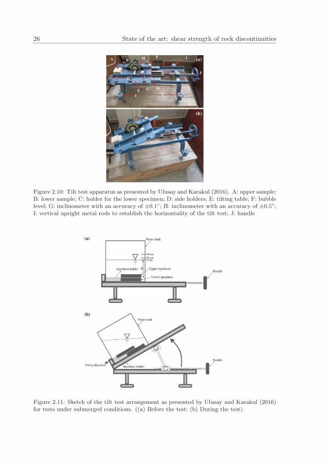
26 State of the art: shear strength of rock discontinuities
Figure 2.10: Tilt test apparatus as presented by Ulusay and Karakul (2016). A: upper sample;B: lower sample; C: holder for the lower specimen; D: side holders; E: tilting table; F: bubblelevel; G: inclinometer with an accuracy of ±0.1◦; H: inclinometer with an accuracy of ±0.5◦;I: vertical upright metal rods to establish the horizontality of the tilt test; J: handle
Figure 2.11: Sketch of the tilt test arrangement as presented by Ulusay and Karakul (2016)for tests under submerged conditions. ((a) Before the test; (b) During the test).

Conclusions of this chapter 27
Last contributions in this area have been carried out by some authors who haveput efforts on a better understanding of tilt test results through different methods(Jang et al., 2018) taking advantage of upgraded direct-shear-test, compression-testand tilt-test apparatuses, like that shown in Figure 2.12. Other recent studies werefocused on the estimation of the basic friction angle of rock surfaces through three-core-arrangement tests (Li et al., 2017; Zhang et al., 2019) from an experimental pointof view.
Figure 2.12: Modern tilting table designed by AceOne Tech as presented in Jang et al. (2018).
2.5 Conclusions of this chapter
In this chapter, an overview of the shear strength of rock discontinuities is presented.Firstly, a general description of the mechanical properties of discontinuities is carriedout, giving way to a review of the main shear strength criteria for discontinuities.Then, different proposals for tilt-test arrangements and procedures developed so farwere analysed.
All shear strength criteria can be considered as sophisticated or evolved versionsof the Mohr-Coulomb criterion (Coulomb, 1776). This means that, for planar, smoothrock surfaces, the majority of these criteria become a Coulomb-type equation, in whichthe shear strength depends only on the normal stress and the basic frictional compo-nent.
In the 70’s, a great advance was observed with the appearance of the Barton’sshear strength criterion (Barton, 1973), later updated as the Barton-Bandis criterion(Barton and Bandis, 1982), which allowed rather rigorous and practical estimation ofthe shear strength of discontinuities through simple equation inputs. Another charac-teristic was being able to take into account the scale effect.

28 State of the art: shear strength of rock discontinuities
Despite this fact, it has been observed that the majority of studies devoted todevelop the shear strength equations have particularly put many efforts on rock sur-face characterisation of the joints. Nevertheless, a reliable estimation of the basicfriction angle as well as a straightforward description of the procedure to obtain thatparameter are frequently omitted in the corresponding papers reporting the new shearcriteria. Another fact to keep in mind is that many of the inputs for the describedcriteria have little physical meaning.
It has been detected a general disregard for a reliable estimate of the basic frictionangle in a good number of the shear strength criteria, as well as a general omission ofthe procedures at issue. Additionally, it is considered that, in spite of the efforts madeby several authors in the estimation of the basic friction angle by tilt test, a generalizedprocedure that serves for a standard calculation of the parameter is missing, a gapthat this PhD thesis aims to fill.

Chapter 3
Experimental studies ontilt-test
The present chapter describes the experimental program undertaken to determinethe influence of different factors (such as mineralogy and rock type, type of saw bladeand cutting velocities, specimen geometry, tilting rate, wear and roughness) on tilt-test results. The study is complemented by a preliminary numerical study carried outwith UDEC (Itasca, 2016), which aimed at assessing the stress distribution on differenttilt-test arrangements. Moreover, the experimental results obtained from a benchmarkexperiment in which the author of this dissertation has taken part are presented. Mainresults presented in the current chapter have been published in the following researchpapers:
• Perez-Rey, I., Alejano, L. R., and Muralha, J. (2019a). Experimental Study of Fac-tors Controlling Tilt-Test Results Performed on Saw-Cut Rock Joints. Geotech-nical Testing Journal, 42(2):307–330
• Alejano, L. R., Muralha, J., Ulusay, R., Li, C. C., Perez-Rey, I., Karakul, H.,Chryssanthakis, P., Aydan, O., Martınez, J., and Zhang, N. (2017). A BenchmarkExperiment to Assess Factors Affecting Tilt Test Results for Sawcut Rock Surfaces.Technical Note. Rock Mechanics and Rock Engineering, 50(9):2547–2562
3.1 Introduction
Tilt tests involve the progressive inclination of two rock surfaces until sliding occurs,as in the case of slab-like specimens (Alejano et al., 2012a, 2018a), the case of three-core method with two linear contacts (Stimpson, 1981; Li et al., 2017), or the caseof the two-core method with only a single linear contact (Barton, 2011; Ruiz and Li,2014). The sliding mechanisms affecting the rock specimens are governed by a rangeof factors (several illustrated in Figure 3.1), including geological origin, degree ofweathering, specimen preparation, surface cutting and finishing, specimen shape andsize, the tilting rate, equipment vibrations, the number of repetitions and surface wear.
29

30 Experimental studies on tilt-test
Several authors have studied the influence of these different factors in evaluatingthe basic friction angle of rock surfaces using tilt tests. In this section, the main as-pects controlling tilt test results will be assessed based on former references but mainlyfounded on laboratory and numerical studies carried out by the author of the presentdissertation.
Figure 3.1: Factors controlling the basic friction angle of saw-cut rock surfaces in laboratorytilt tests.
3.2 Mineralogy and rock type
One intrinsic characteristic of tested materials is the mineralogical composition, whichhas been reported by various studies to affect the frictional behaviour of rock sur-faces (Ramana and Gogte, 1989; Ulusay and Karakul, 2016). This factor is especiallysignificant when analysing nominally planar rock surfaces, such as those obtained bysaw-cutting. In addition, according to Cruden and Hu (1988), the frictional behaviourof some carbonated rock specimens also present dependence on the grain size.
Ramana and Gogte (1989) studied how rock nature and composition influence thefrictional behaviour of the rock surfaces of rock sampled from several different placesin India. Using a form of tilt test performed with rectangular-based slabs, they studiedboth fractured and saw-cut planar surfaces in order to analyse static friction coeffi-cient dependence o mineralogy, including twelve different rocks associated with theobserved frictional properties (Table 3.1).
According to Table 3.1, carbonated rocks may yield higher friction angles than, forinstance, metamorphic quartzites, granites, or dolerites with higher quartz contents.

Saw blades and cutting velocities 31
Table 3.1: Coefficient of sliding friction and the corresponding basic friction angle for saw-cutrock (adapted from Ramana and Gogte (1989)).
.Rock type μk φb[
◦] Rock type μk φb[◦]
Grey granite 0.54 28Sandstone
0.62 310.73 360.42 23
Pink granite 0.48 25Limestone
0.69 340.62 32
Gneissic granite 0.46 24 Dolerite 0.44 23Charnockite 0.46 24 Biotitic quartzite 0.53 28
Deccan basalt (fresh)0.45 24
Micaceous phyllite0.53 28
0.55 28Deccan basalt (weathered) 0.48 25 Amphibolite 0.53 28
Nonetheless, the influence of rock mineralogical composition on tilt test results has tobe interpreted with caution because other features may affect the frictional behaviourof rock specimens. Although aspects related to rock lithology cannot be controlledby rock mechanics practitioners, understanding them may be of help when analyzingtilt-test results.
3.3 Saw blades and cutting velocities
The cutting process is another factor influencing tilt-test results. Roughness and pla-narity are affected by the type and condition of the saw blade used to obtain testsurfaces, and the final surface condition can be affected by the cutting speed andforces exerted by the rock slab against the blade. Figure 3.2 illustrates how usingdifferent blade types to obtain tilt test specimens, results in apparently flat planarsurfaces looking rather different under a binocular microscope.
From a mechanical perspective, it is important to assure that the sliding processoccurs under compressive stresses, as these can be better controlled when specimenshave faces as planar as possible. This feature is related to geometrical considerationswhich will be assessed in the section 3.4.
A somewhat unavoidable consequence of the common rock cutting processes is re-lated to imperfectly flat contact surfaces. When performing some tests for the presentresearch, mismatched zones were detected, particularly at slab edges (Figure 3.3a).This type of flaw is associated with blade vibrations at the start and at the end ofthe cutting process, when blade spin is less stable. After several tests, it was foundthat this effect could be avoided by using two waste-rock blocks placed in front of andbehind the original slab. Clamped together, the three blocks form a solid set thatstabilizes and guides the saw blade an so avoids defective edges and greatly reducesthe non-planarity of the final surface (Figure 3.3b).
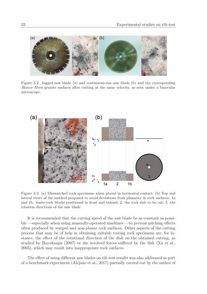
32 Experimental studies on tilt-test
Figure 3.2: Jagged saw blade (a) and continuous-rim saw blade (b) and the correspondingBlanco Mera granite surfaces after cutting at the same velocity, as seen under a binocularmicroscope.
Figure 3.3: (a) Mismatched rock specimens when placed in horizontal contact; (b) Top andlateral views of the method proposed to avoid deviations from planarity in rock surfaces: 1aand 1b. waste-rock blocks positioned in front and behind; 2. the rock slab to be cut; 3. therotation directions of the saw blade
It is recommended that the cutting speed of the saw blade be as constant as possi-ble —especially when using manually-operated machines —to prevent pitching effectsoften produced by warped and non-planar rock surfaces. Other aspects of the cuttingprocess that may be of help in obtaining suitable testing rock specimens are, for in-stance, the effect of the rotational direction of the disk on the obtained cutting, asstudied by Buyuksagis (2007) or the involved forces suffered by the disk (Xu et al.,2003), which may result into inappropriate rock surfaces.
The effect of using different saw blades on tilt-test results was also addressed as partof a benchmark experiment (Alejano et al., 2017) partially carried out by the author of

Specimen geometry and involved tilt-test stresses 33
the present dissertation, as it will be presented in Section. Combining statistical tech-niques, tilt-test results for four rock types (granite, basaltic andesite, limestone andquartzite) were analysed and found to be reproducible, provided saw blades with dia-mond counts in the range of 0.6–1.0 carat/cm3 and grit sizes of 50–100 Mesh US wereused to cut. This finding is in line with performance studies of rock cutting processes(Ersoy and Atici, 2004). To conclude, diamond saw blades with those characteristics,along with constant feed rates, would enable sufficiently representative rock surfacesto be obtained for tilt testing.
3.4 Specimen geometry and involved tilt-test stresses
The earliest studies of the influence of the geometry of slab-like specimens on tilt-testresults were carried out by Hencher (1977), who developed an analysis of the slidingbehaviour of prismatic wooden blocks that was later extended to rock sliders. Thesliding mechanisms of these specimens were studied in terms of stress distribution,surface wear, and influence of the specimen position during testing, as well as in termsof the normal loads applied to both wooden and rock blocks. Hencher (1977) formu-lated two expressions for calculating the rear (σA) and front (σB) compressive stressesexerted by a prismatic block with weight, W, resting on a plane inclined β degrees.
σA =W
lb cosβ
(1− 3h
ltanβ
)(3.1)
σB =W
lb cosβ
(1 +
3h
ltanβ
)(3.2)
According to Equation 3.1, in order to theoretically ensure that all stresses on thecontact surface are compressive during sliding, the length-to-height ratio of the upperslab must be greater than 3× tanβ.
Alejano et al. (2012a) undertook a detailed study aimed at assessing basic fric-tion angle results obtained for different geometrical shapes of specimens. Tested werecylindrical-shaped specimens obtained from rock cores (Stimpson, 1981), lengthwise-cut cylinders, disc-shaped (Brazilian test) specimens and slab-like specimens. Theyalso recommended the use of slab-like specimens (exceptionally, lengthwise-cut rockcores) presenting surfaces greater than 50 cm2 and length-to-height ratios (l/h) greaterthan two (at least) to ensure sufficiently regular normal stress distributions under com-mon test conditions. This is particularly important when testing rocks with relativelyhigh mineralogical friction coefficients.

34 Experimental studies on tilt-test
Figure 3.4: Compressive stress distribution on the base of a prismatic block on an inclinedplane [adapted from Hencher (1977)].
Figure 3.5: Different configurations for laboratory tilt testing: (a) cylindrical specimens(Stimpson, 1981), (b) a lengthwise-cut cylinder, (c) disc-shaped specimens, and (d) slab-likespecimens [adapted from Alejano et al. (2012a)].

Specimen geometry and involved tilt-test stresses 35
Some simple analytical approaches, based on basic Mechanics, have been presentedhere to estimate normal stress distributions along the contact boundary of two slab-likerock specimens (Hencher, 1976). Other studies for oval or circular-section specimens,based on foundation-design theories were carried out by (Kim et al., 2016). As pre-viously indicated, somewhat simple formulation to estimate maximum and minimumstresses exerted by a rectangular-based specimen resting on an inclined plane is pre-sented by Equations 3.1 and 3.2. Although these analytical solutions are simple andsomewhat useful, they do not represent a practical way to analyze geometrical scenar-ios beyond perfectly-defined prismatic slabs; that is, for example, in the case of partsof the upper slab overhanging (Figure 3.6) or for testing specimens with geometricalflaws.
Figure 3.6: Detail of the overhanging part of the upper specimen when subjected to a tilttest carried out with two equi-dimensional specimens.
In order to better understand normal stress distributions for these situations andto complement the previous assessment of the influence of geometry, very simple nu-merical analyses were carried out by using UDEC 6.0 (Itasca, 2016), as introduced inthe following section 3.4.1.
3.4.1 Numerical analysis of normal stress distributions for tilt-test specimens of different geometry
Although the mechanics of the tilt-test is, a priori, quite simple, there are certainaspects that deserve further study since they can help on understanding test results.Figure 3.7 shows four different sketches illustrating some common situations that, asaforementioned, could arise when performing tilt tests on saw-cut rock surfaces: model(a) (Figure 3.7a) corresponds to a conventional lay out (two blocks of equal size, oneresting above the other); model (b) (Figure 3.7b) presents different size for the upperand lower (longer) block, allowing a constant sliding surface for all the test; model (c)(Figure 3.7c) is intended to represent a defective upper specimen, as a consequence ofbad cutting at the front edge; the last one model (d) (Figure 3.7d), aims to representan interlocking of the upper specimen (i.e. due to an untrimmed grain) at the back.

36 Experimental studies on tilt-test
Figure 3.7: Models proposed for the assessment of the influence of geometrical features (mea-surements are in mm and red arrow indicates sliding direction).
The presented numerical simulation aims at reproducing the successive inclinationof the blocks observed during the development of a real tilt test. Instead of tiltingthe blocks, what was proposed for the present case simply involved the rotation ofthe gravity vector by one-degree (◦) steps. This rotation cycle was implemented from0◦ until a value slightly greater (28◦) than the selected parameter jfriction = 26◦
(Itasca, 2016). Figure 3.8 shows unbalanced forces for each 10000 steps and Figure3.9 evidences, by representing x-displacement, the sliding of the upper block when thefriction component is overpassed.
Figure 3.8: History of unbalanced forces versus number of cycles.

Specimen geometry and involved tilt-test stresses 37
Figure 3.9: History of x-displacements versus number of cycles.
Tilting mechanism was implemented by a counterclockwise rotation of the gravityvector in steps of a degree. Then, all models were computed to analyze normal stressdistributions on the contact. Figure 3.10 corresponds to a UDEC plot showing ge-ometry for the simplest case, simply considering two rectangular-based slabs of equallength subjected to the same forces as experience in a tilt test.
Figure 3.10: Geometry of the simplest model (two rectangular-based slabs of equal length).
As can be appreciated in Figure 3.10, the partial sliding of the upper specimen isattained. Part of the upper block overhangs similarly as presented in Figure 3.6. Ac-cording to Figure 3.11, the normal stress distribution along the boundary is displayed.The maximum value reaches 2.446 kPa and the minimum value is 0.272 kPa, locatedat the front and rear contacts between the two specimens, respectively.

38 Experimental studies on tilt-test
Figure 3.11: Corresponding normal stress distribution along the contact surface for specimensanalysed in the model presented in Figure 3.10
Figure 3.12 shows a different lay-out for the test. In this case, a longer plane ofsliding (lower specimen) is used. Compressive normal stress along the contact surfacesis provided in Figure 3.13 where it can be appreciated a linear stress distribution allthroughout the contact surface. A maximum stress of approximately 0.774 kPa isexerted by the upper block at the front contact edge and a minimum stress equal to0.284 kPa at the rear edge.
Figure 3.12: Geometry of the model considering a longer lower (static) specimen

Specimen geometry and involved tilt-test stresses 39
Figure 3.13: Corresponding normal stress distribution along the contact surface for specimensanalysed in the model presented in Figure 3.12
Figure 3.14: Geometry of the model with a cutting flaw at the front.
A cutting flaw had commonly been detected during the obtaining of some rectangular-based rock specimens (Figure 3.3). A reduction of specimens’ height was observed dueto an uncontrolled vibration of the sawblade, particularly affecting the initial partunder cutting. Figure 3.14 depicts the already mentioned flaw, implemented as a pro-gressive reduction of the upper specimen’s height along 20 mm at the front side, froma maximum aperture of 1 mm until the contact is attained.

40 Experimental studies on tilt-test
As can be appreciated in Figure 3.15, this flaw has a direct effect on compressivestresses along the contact, generating a non-linear distribution. The maximum exertedstress can be observed at the front, with a value of 1.923 kPa, reaching a null value atthe rear part of the specimen contact.
Figure 3.15: Corresponding normal stress distribution along the contact surface for specimensanalysed in the model presented in Figure 3.14
The last proposed model intends to represent a particular effect detected by theauthors while carrying out actual tests. This effect is related to a random presence ofabnormally-high values —statistically interpreted as outliers (Perez-Rey et al., 2018).These abnormally-high values may occur due to the interlocking between untrimmedgrains and/or grooves, as a result of a defective cutting process.
This effect is presented in Figure 3.16 as a slight protrusion located at the back ofthe boundary. Figure 3.17, in which normal stress is displayed against the length ofthe specimen, shows the loss of compressive stress at the back, reaching a maximumof 1.152 kPa at the front edge contact. If the normal stress is plotted just for theback flank of the defect (Figure 3.18), a relevant local increase of the normal stress isevidenced, with a maximum value of 3.137 kPa.

Specimen geometry and involved tilt-test stresses 41
Figure 3.16: Geometry of the model showing an untrimmed grain at the back.
Figure 3.17: Corresponding normal stress distribution along the contact surface for specimensanalysed in the model presented in Figure 3.16

42 Experimental studies on tilt-test
Figure 3.18: Corresponding normal stress distribution at the back flank of the grain in themodel presented in Figure 3.16
Figure 3.19 summarizes all normal stress results in kPa for all the considered scenar-ios. Black line represents compressive stresses for the model considering two specimenswith equal length; red line also indicates compressive stresses but for a specimen slid-ing on a longer lower slab. Blue line represents a specimen with a 20-mm cutting flawat the frontal edge and the magenta line holds for a specimen presenting a defect at theback (idealization of interlocking contact surfaces due to the presence of untrimmedgrains).
0 0.01 0.02 0.03 0.04 0.05 0.06 0.07 0.08Relative (x-axis) coordinates referred to the upper specimen [m]
0
0.5
1
1.5
2
2.5
3
3.5
Nor
mal
str
ess
Equal length sp.Diff. length sp.Front flaw sp.Back flaw sp.
Figure 3.19: Normal stress [kPa] plotted at each contact, for all cases analysed

Specimen geometry and involved tilt-test stresses 43
All results for maximum and minimum compressive stresses recovered from thisUDEC-based numerical study are presented in Table 3.2. Location for each of themalong the contact boundary (y = 0.025 m) is provided.
Table 3.2: Maximum and minimum normal stresses and their locations on the boundary (y= 0.025 m for all models). Referred models correspond to those shown in Figure 3.7.
Model Max. normalstress (MNS)
MNS location (x-axis)
Min. normalstress (mNS)
mNS location (x-axis)
[kPa] [m] [kPa] [m]
(a) 2.446 x = 0 0.272 x = 0.07(a) 0.774 x = 0.035 0.284 x = 0.016(a) 1.923 x = 0.057 0 x = 0.107(a) 2.446 x = 0 0.272 x = 0.05
3.137 x = 0.065 3.023 x = 0.07
Theoretical approaches addressed to estimate the normal stress distribution alongcontacts between two-slab like specimens, evinced a linear decay for the compressivestress. This happens from the front edge (maximum exerted stress) to the rear allalong the contact boundary. This statement holds for rectangular-based specimenspresenting length-to-height ratios l/h > 3 × tanβ. Nevertheless, these solutions lackof practicality when applied to complex geometries or when specimens are affected bythe process of cutting, that is, slightly modified geometries (a common fact in rockmechanics laboratories).
According to compressive-stress distributions obtained in the models, it is evi-denced that for two specimens of equal length (first considered scenario), a relevantincrease at the frontal contact area arises. This is attributed to the overhanging part ofthe upper specimen. For multiple sliding series on the same surface, this stress increasemight relevantly wear the sliding surface, especially at the frontal part. The unde-sired effect of wear causes a decrease on basic friction angle as number of test increases.
For the second proposed scenario (a sliding specimen of smaller length than thelower one), it can be observed that for specimens fulfilling recommended length-to-height ratio, the stress distribution is completely linear and always compressive duringsliding. Difference between maximum and minimum stress is roughly 0.5 kPa. Thissomewhat smooth stress distribution is considered the most appropriate for carryingout tilt tests.
The effect of a cutting flaw affecting geometry of the upper specimen has beenalso simulated (third considered scenario). This flaw is associated to the uncontrolledswinging of the sawblade when starting the specimen cutting. Based on experimentalobservations, a height reduction of the upper specimen had been detected and thoughtto affect stress distribution. As deduced from the stress distributions obtained withthe numerical simulation, this geometry causes a relevant increase on the compressivestress at the front edge, leaving the back part of the sliding specimen without load.

44 Experimental studies on tilt-test
Last model aims to represent a test where specimens become interlocked, by thepresence of untrimmed grains or grooves caused by an uncontrolled cutting. Even fornominally flat saw-cut rock joints, which can seem planar for the naked eye, a slightinterlocking of few grains will obviously produce overestimation of the basic frictionangle. Consequently, normal stress increases on the zones where the interlocking oc-curs.
Based on this numerical study, rectangular-based specimens allocated to carry outtilt tests should present surfaces as planar as possible, obtained through controlled sawcutting. Length-to-height ratios of the specimen (l/h) greater than 4 complementedwith longer specimens at the bottom of the arrangement (or a limitation of the totalsliding run) help on achieving completely compressive-stress distributions on the con-tact.
3.4.2 Influence of specimen width on tilt test results
Following up on several geometric studies (Hencher, 1977; Alejano et al., 2012a) andintending to analyze the effect of specimen width on tilt-test results and the scale effectsomehow, an experimental study were planned during the stay of the author of thisdissertation at the ’National Laboratory for Civil Engineering’ (LNEC) in Lisbon (Por-tugal), in the months from March to May 2017. This experimental program includedthe preparation of seven pairs of a medium-grain granite specimens, with a 500-mm-diameter segmented saw blade. The mean dimensions and the corresponding massesof the specimens are presented in Table 3.3. For each pair of specimens —except forblocks 12 A-12 B and 12 C-12 D—, the two possible contact surfaces correspondingto each cut side were tested 15 times and cleaned with a soft brush after each rep-etition. This yields a total of 12 series, with a total number of 180 tilt tests carried out.
Table 3.3: Mean dimensions and masses of 14 specimens used for assessing the specimen-widtheffect on tilt-test results.
Specimen L, mm b, mm h, mm l/h Mass, g
11A 188.0 161.0 22.48 8.4 1,781.011B 180.7 161.6 20.89 8.6 1,601.534A 155.0 132.7 21.12 7.3 1,150.534B 155.7 131.7 20.91 7.4 1,131.523A 153.3 119.7 22.37 6.9 1,096.023B 155.0 119.0 22.24 7.0 1,081.012A 161.0 86.2 38.37 4.2 1,342.512B 160.7 88.5 33.59 4.8 1,184.012C 152.3 89.3 23.53 6.5 805.012D 153.0 95.0 29.66 5.7 879.013A 154.8 61.7 22.45 6.9 566.513B 155.0 60.0 22.05 7.0 537.514A 155.0 48.2 20.91 7.4 411.014B 155.7 48.5 21.06 7.4 425.0

Specimen geometry and involved tilt-test stresses 45
As can be appreciated in the graphs in Figure 3.20, the experimental results indi-cated no relationship or dependence trends between specimen size and sliding anglevalues. Figure 3.20a shows all median values from the first five tests in each series untilthe whole 15 tests are carried out. Three of a total of twelve series presented abnormalresults that went against the general trend. For the smallest series (13Ai-13Bi), thiswas because of poor matching between the upper and lower specimens, particularlyat the edges (as illustrated in Figure 3.20a). This effect possibly leads to prematuresliding as a consequence of a slight toppling of the upper block.
In contrast, higher values than expected were obtained for two other series (12A-12B and 23As-23Bs), in relation to the mean and median of the whole dataset, andthis was thought to be due to irregularities observed on the surface and also due tothe shape and weight of a single specimen (particularly, 12B). This would exemplifythe influence of the cutting process and specimen geometry on results, highlightingthe need to consider such factors when carrying out tilt tests.
Figure 3.20: (a) Evolution of median values for the datasets for the different specimens; (b)median of sliding angles versus specimens’ width; and (c) histogram of frequencies for allrepetitions and fitted normal distribution curve (mean and standard deviation provided).
Figure 3.20b depicts the medians of all 15 tests carried out with each pair of spec-imens, which are represented against specimen width (this represented in terms ofmaximum width of larger specimen, b = 188 mm). As can be seen, there is no evidenttrend, which indicates that there is no sliding friction dependence on width for theanalyzed geometries. Supporting this fact, for raw values plotted by a histogram of

46 Experimental studies on tilt-test
frequencies, around 60% of sliding angle values fall within the range of 24◦–27◦ andmedian values also tend to fall within the same range (Figure 3.20c). It can there-fore be concluded that specimens fulfilling both the surface conditions recommendedin Alejano et al. (2012a) and the length-to-height ratios of, at least, two, will yieldsufficientely reproducible and representative tilt-test results. Regarding practical as-pects, provided the specimen width b is greater than 55 mm, it is recommended thatlengthwise-cut standard NX rock cores be used for testing when necessary.
3.5 Test platform tilting rate and induced vibrations
3.5.1 Tilting rate
The characteristic tilting movement in a tilt test can be carried out at different tiltingrates, with the possibility that this procedure affects the results. Tilt tests are com-monly run in laboratorioes —both for research and engineering purposes —at differentvelocities, ranging from hundreths to a few tenths of degree per second (Cruden andHu, 1988; Alejano et al., 2012a; USBR, 2009; Gonzalez et al., 2014; Ruiz and Li, 2014).
To assess these different practices, an experiment that consisted of 20 series of tilttests performed at different angular velocities was conducted using a motorized tiltingtable and tilting rates of 2◦, 4◦, 7.5◦, 12.5◦ and 25◦ per minute —that is, embracingthe entire range covered in the previously mentioned references.
A total of 20 specimens measuring 115 × 100 × 25 mm each were cut from two pri-mary granite rock blocks of 300 × 120 × 120 mm. To take the maximum advantage ofthe available surfaces, rock specimens were tested on both sides. A 350-mm-diameterand 3.4-mm-thick saw blade used for cutting had 23 teeth of a bronze alloy matrix withdiamond concretion of approximately 6 carat/cm3 and a teeth grit of approximately50-60 Mesh US.
Lithologically, the rock was a moderately weathered, medium-grained granite,which is very common in the northwest of the Iberian Peninsula. This granite hasa density of 2.61 g/cm3, a mean uniaxial compressive strength (UCS) value of roughly75 MPa, and a tensile strength of about 7 MPa. Five tilt tests were included in eachseries, and raw test results are grouped by tilting rates in Table 3.4.
To study dependence on tilting rates, test results were simply represented againstangular velocities and test repetitions. Adjusting a linear function for both datasets, itcan be observed that there is no dependence between basic friction angles and angularvelocity; this fact is mathematically evidenced by a low coefficient of determination,R2 = 0.0517 (Figure 3.21a). Nevertheless, when test results are plotted against theircorresponding repetitions, a clear decaying trend can be observed (Figure 3.21b) inthe sliding angles, that is associated with a wearing effect on the rock surfaces that isdue to repeated sliding. In this case, the coefficient of determination is much closer to1 R2 = 0.939, what means a better correlation between results and the linear fit.

Test platform tilting rate and induced vibrations 47
Table 3.4: Basic friction angles obtained from tilt tests performed at different tilting rates.
RepetitionsSeries ω [◦/min] φb[
◦] φb[◦] φb[
◦] φb[◦] φb[
◦]
TR-1 25 32.5 30.9 30.2 29.8 27.6TR-2 25 29.0 26.3 25.4 25.3 25.4TR-3 25 31.3 32.7 31.7 31.5 31.2TR-4 25 30.9 31.1 30.7 30.8 29.5TR-5 12.5 29.2 29.2 31.0 28.9 28.9TR-6 12.5 27.5 26.8 27.3 25.4 29.1TR-7 12.5 27.1 27.2 26.4 26.7 27.2TR-8 12.5 29.1 31.3 27.5 26.1 26.1TR-9 7.5 30.7 30.8 29.4 30.0 29.6TR-10 7.5 29.2 29.4 27.6 25.6 28.6TR-11 7.5 32.2 29.6 30.7 29.8 28.0TR-12 7.5 29.3 28.0 27.9 29.1 30.8TR-13 4 31.1 32.2 31.0 30.4 30.2TR-14 4 30.6 30.6 28.0 26.7 26.6TR-15 4 28.9 28.7 30.8 29.6 30.2TR-16 4 30.1 30.3 30.7 29.8 28.9TR-17 2 32.2 30.0 28.6 29.9 26.6TR-18 2 30.9 27.9 27.8 26.3 27.7TR-19 2 30.2 25.6 32.1 24.1 23.4TR-20 2 30.3 30.7 28.5 27.6 27.8
Boxplots were used to analyze the dispersion of results for both the completedatasets and each selected tilting rate and repetition (Figure 3.22).
This kind of representation depicts numerical data groups using quartiles and indi-cates variability of results using vertically extended lines (whiskers) and single pointsto show outliers. The trend and conclusions are the same as for Figure 3.21.
The one-way analysis of variance test (ANOVA) was used to analyze the depen-dence between the sliding angle and the tilting speed of the tilting table so as to checkwhether the results of different tests carried out at different tilting rates (from 2◦ to25◦/min) belonged to the same statistical population.
As a consequence of consecutive sliding, wear affects rock contacts and results indifferent surface conditions for each testing stage. This fact makes it necessary toapply a correction to the ANOVA to be able to analyze statistical belongingness to apopulation. Thus, based on the linear equation presented in Figure 3.21b, values werefirst adjusted by adding to each raw result the corresponding value of the slope timesthe repetition. This added value represents the angular decay or loss for each testingstage. The effect of wear detect here, will be analysed in more detail below.

48 Experimental studies on tilt-test
Figure 3.21: (a) Sliding angles and tilting rates; (b) sliding angles and test repetitions (coef-ficients of determination are shown for group averages)
Figure 3.22: Boxplot representations (a) for sliding angles and tilting rates (b) for slidingangles and test repetitions.

Wear and time 49
Once raw tilt test results were corrected so as to make data presumably dependentonly on tilting rates, the ANOVA test was applied to this new dataset, which wasmade up of the mean results of four series for each tilting rate (leaving five new groupsof four data items). After applying ANOVA for the significance level of α = 0.05(commonly used in statistical studies) and after taking into account F , which is thevalue of the statistic for the considered degrees of freedom (four between groups and15 within groups for this case), the resulting test output is F (4, 15) = 1.377, withp = 0.289. Because this p-value is greater than the significance α, it can be statedthat the tilting rate —within the selected range of angular velocities —does not affecttilt-test results.
This experimental study along with the statistical interpretation of results demon-strate that tilting rates in the range of 2◦ to 25◦/min —values commonly found inother studies (Cruden and Hu, 1988; Ruiz and Li, 2014; Gonzalez et al., 2014; Alejanoet al., 2012a; USBR, 2009) —do not affect basic friction angle results obtained from tilttests, at least when a motorized table is used. To account for both the reliability andpragmatism of the testing procedures, it would appear that tilting rates in the rangeof 10◦ to 15◦/min seem appropriate for tilt tests. In parallel to these experiments,it was observed that the effect of wear affected results to a relevant degree, even fora reasonably low number of test repetitions, and especially for moderately to ratherweathered rocks. This, therefore, is another effect that should be taken into accountwhen analysing tilt test results.
3.5.2 Vibrations and accelerations
Recent experiments, partially carried out by the author of the present dissertationand presented in Alejano et al. (2017) suggest that conclusions regarding tilting ratesmay not hold when using hand-operated tilting platforms because vibrations (or ac-celerations) may be induced during tilting, although these can be measured by ac-celerometers (nowadays, these are available as free apps for standard smartphones oras low-cost sensors (Muniz-Menendez et al., 2019)). As a practical recommendation,accelerations smaller than 0.005g can be considered negligible in terms of tilt test re-sults carried out with slab-like specimens.
3.6 Wear and time
The basic friction angle is a parameter representative of the frictional strength of aplanar, unfilled and non-weathered joint, as defined by Barton (1973) and Barton andChoubey (1977). According to these authors, a planar rock joint will present a nullJRC value and nonweathering can be assumed when the joint UCS corresponds tothat of sound rock. A surface that satisfies these conditions can be obtained by sawcutting. Nevertheless, although a saw-cut rock surface may appear to be planar tothe naked eye, surface microroughness that may affect frictional behaviour will alwaysbe present, as observed in some studies (Krahn and Morgenstern, 1979; Reeves, 1985;

50 Experimental studies on tilt-test
Hencher and Richards, 2015), which highlight the influence of microroughness on thestrength behaviour of apparently planar rock surfaces.
Another factor considered to affect tilt test results is the wear of rock surfaces,which is a consequence of multiple sliding on the same surface or contact. Variousauthors (Hencher, 1976; Gonzalez et al., 2014; Perez-Rey et al., 2019a) have reporteddecaying trends in results when performing tilt tests without allowing rock powder toaccumulate, that is, cleaning the rock surface after each run.
Finally, but not less importantly, the time elapsing between cutting and testingmay have a bearing on the results, as environmental conditions may affect the speci-mens.
3.6.1 Wear
Wear is understood as surface damage, commonly with loss of substance, arising frommechanical contact between two bodies that have suffered progressive damage becauseof sliding mechanisms (Hencher, 1977; Zum Gahr, 1987; Blau, 2016). This effect canbe observed in saw-cut rock surfaces subjected to repetitive sliding, as in the case ofspecimens used to estimate basic friction angle by means of tilt tests.
One of the first studies describing some conclusions on the effect of wear on a rocksurface was carried out by Coulson (1972). Years later, Hencher (1977) developed anexhaustive study describing wear effects as well as other features concerning tilt testson rock surfaces. The effect of removing rock powder produced by friction betweenrock surfaces is particularly addressed. All these features are related with their effecton the estimation of basic friction angle by means of tilt tests.
To study how saw cut rock surfaces are affected by wear and rock powder and toassess how progressive damage may affect basic friction angle results, an experimentwas carried out in the core of this thesis (Perez-Rey et al., 2019a) on three rock types,namely: a serpentinized dunite, an orthogneiss and a migmatite, that where testedas slab-like specimens measuring 100×100×40 mm, 80×110×25 mm and 80×110×40mm, respectively. For each case, 300 repetitions were carried out.
The sliding angles of each rock according to sliding distance were represented inFigure 3.23. In this case, tests were carried out after removal of the rock powder gen-erated after each test for the first 100 runs (serpentinized dunite and orthogneiss) andfor the second 100 runs (migmatite). The remaining tests were carried out allowingrock powder to accumulate between runs.
The trends observed in Figure 3.23 are consistent with the observations made byHencher (1977). Results obtained for serpentinized dunite vay from 30◦ to 10◦ for thefirst 100 tests (with rock powder removed) and move to about 22◦ for the second 100runs (when rock powder is allowed to accumulate). When surfaces are cleaned between

Wear and time 51
tests, the sliding angle drops to a value of around 10◦ after the last 100 repetitions.For orthogneiss, a similar trend can be observed. The sliding angle decreases from 25◦
to 10◦ during the first 100 repetitions (when rock powder is removed) and reaches 20◦
to 24◦ after the second 100 runs (when rock powder is allowed to accumulate). For thelast 100 repetitions, a minimum value of 10◦ is attained when rock surfaces are cleaned.
Figure 3.23: (a) Rock specimens prior to testing. Sliding angles for (b) migmatite, (c)orthogneiss, and (d) serpentinized dunite, according to accumulated sliding distance (dis-placement). Red squares represent tests in which rock powder was removed after each run,and black squares represent tests in which rock powder was allowed to accumulate
The procedure applied to migmatite was the reverse of that used for the two otherrocks. For the first 100 repetitions, rock powder was allowed to accumulate, producingsliding angle results in the range of 25◦ to 32◦. The second 100 repetitions, when rocksurfaces were cleaned after each run, produced a decay in the sliding angle startingat 32◦ and ending at about 10◦. The last 100 runs, which allowed rock powder toaccumulate after each run, obtained values similar to those observed for the first 100repetitions but without surface cleaning (25◦). During these tests of saw-cut rock sur-faces, it should be appreciated that neither the effect of wear, which tends to decreasethe sliding angle, nor the effect of accummulated rock powder between runs, whichtend to increase the sliding angle, is overlooked.
To extend this study, additional tilt tests were performed on three other rock types

52 Experimental studies on tilt-test
(sandstone, granite and slate), cleaning the surfaces between runs (Perez-Rey et al.,2015). Results are presented in Figure 3.24, which depicts decaying trends for all sixrocks. A semi-logarithmic equation was able to capture the sliding angle drop withrespect to sliding distance. The coefficients of determination showed reasonably goodcorrelations of data with suggested expressions.
Figure 3.24: Sliding angle and accumulated sliding distance (displacement) results in semi-logarithmic axes for six different rocks: (a) migmatite, (b) granite, (c) serpentinized dunite,(d) gneiss, (e) slate, and (f) sandstone. Fitting functions and coefficients of determinationfor each dataset are provided.
These tests indicate that tilt tests are affected by the accumulated sliding distance.The decaying trends could be related in some manner with rock abrasiveness and fric-tional strength, as rocks more prone to disaggregation (sandstone) or with soft mineralswithin the group of phyllosilicates (serpentinized dunite) show steeper decaying trendsthan other harder, crystalline rocks, like granite. These results suggest that only theinitial tilt tests truly represent the frictional behavior of planar discontinuities. Weareffects tend to be complex and are associated with the types of minerals forming thegrains, grain size distribution, and contact behavior between grains. Although a pol-ishing effect systematically occurs in all rock surfaces, the evolution of the effect andits impact on the basic friction angle is difficult, if not impossible, to control. Withthe aim of removing this effect, the authors propose that wear be avoided as muchas possible when performing tilt tests. This can be achieved in the practical way ofblocking the sliding distance of the upper rock slab by allowing only a slight displace-ment amounting to 5% to 10% of the total length of the specimen. This approach alsoprevents the upper block from slightly toppling at the base edge when sliding —notonly an undesired effect regarding test mechanics but also an aggravator of wear effects.

Wear and time 53
3.6.2 Time
The observation of anomalous values for a number of tests on specimens that had beenstudied years previously piqued the interest of the author regarding the possible effectof time on tilt test results. Specifically, a systematic decrease of between 5 and 10 wasobserved for previously measured angles for Blanco Mera granite specimens. Becausethe number of tests performed on those specimens was not clear, it was decided toconduct an experiment to further analyze whether these decreases were due to thepassage of time or associated with repetitive sliding (wear).
This experimental program involved the preparation of six pairs of slab-like speci-mens, measuring 150 × 50 × 50 mm, kept under controlled laboratory conditions fromthe cutting stage until test completion for six months: temperature in the range of 20◦C–24◦C and relative humidity in the range of 45–53 %. One pair (B601-B602) wastested six times (that is, once a month), a second pair (B603-B604) was tested fivetimes (again, once a month starting a month after the first pair), and so on to the lastpair (B611-B612), which was tested only once (five months after the first pair). Theoutcome was a total of 105 values, with results as shown in Figure 3.25.
Figure 3.25: Test series carried out at different times during a six-month experimental pro-gram. The red line indicates a series included as representative of a nonplanar and irregularsurface resulting from incorrect saw cutting. Each point represents a mean of five repetitions.
The test series depicted in Figure 3.25 show that first values of each series werevery close, lying approximately within a 2◦ window independently of the momentthey were tested. This would indicate that time (on a monthly scale) does not affecttilt test results. Nevertheless, even for a scant number of repetitions, the effect ofwear is evident as sliding angle values are lower. That said, this conclusion does not

54 Experimental studies on tilt-test
apply to series B603-B604, as initial values were somewhat lower than for the otherseries. This is explained by bad matching between rock specimens resulting frominappropriate cutting, which only highlights, yet again, the importance of geometryand cutting in obtaining representative results.
3.7 Participation in a benchmark experiment
3.7.1 Introduction
This section contains the experimental results obtained from a benchmark experimentperformed by four laboratories (University of Vigo, Spain; National Laboratory forCivil Engineering, Portugal; Hacettepe University, Turkey and Norwegian Universityfor Science and Technology (NTNU), Norway) in which the author of the present dis-sertation has participated by carrying out and analysing about 490 tilt tests. Thisexperiment was intented to shed light on the observed variability in sliding angle re-sults from tilt tests. The work —entitled A Benchmark Experiment to Assess FactorsAffecting Tilt Test Results for Sawcut Rock Surfaces —has been published in theformat of Technical Note’ in Rock Mechanics and Rock Engineering journal (Alejanoet al., 2017).
A large number of tilt tests in different conditions have already been carried out,including those reported in Alejano et al. (2012a) and in some more recent stud-ies (Gonzalez et al., 2014; Ruiz and Li, 2014; Ulusay and Karakul, 2016; Li et al.,2017) as well as several other tests not presented in the literature. Results suggest areasonable degree of reproducibility of tilt testing under controlled conditions. Theaforementioned studies typically used different cutting machines, tilting tables andtesting procedures. It was therefore deemed interesting to check reproducibility byanalysing tilt test results carried out in different laboratories in very similar controlledconditions, in order to analyse how and why results were different. The initial ideawas to test 7 contacts of 7 specimens of a particular rock type (granite) 7 times, inthe different cutting and tilting conditions inherent to the equipment from each labo-ratory. However, 3 other rock types (limestone, quartzite and basaltic andesite) werealso tested under 3 or 4 different conditions to take into account possible differencesresulting from different mechanical characteristics, associated with the type of rock.A total of 1078 tilt tests were carried out among the four laboratories.
The main objectives of the experiment were to identify and single out features thatsignificantly affect tilt test outcomes (presented within this section) and to assess thereproducibility of tests performed in different laboratories (Chapter 4).
3.7.2 Experimental approach
The authors prepared a good number of sample blocks of the same rock with dimen-sions 30 × 8 × 7 cm and weight 4-5 kg per block (Figure 3.26) that could be easilymailed to the 4 laboratories that participated in the multi-laboratory experiment. Thebenchmark procedure was to ask each laboratory to cut 7 slab-like specimens with di-

Participation in a benchmark experiment 55
mensions of about 8×7×2.5 cm using the own saw machines and to perform tilt testsusing the available tilting tables (Figures 3.26b and c). Thus, each slab-like specimenwould have 2 faces with a surface of approximately 56 cm2 to carry out tilt tests.This area is slightly over the recommended value of 50 cm2 established in previousexperiments to ensure a large enough tilt surface and to avoid problems related to thecurvature of the saw-cut surfaces (Alejano et al., 2012a). The slab specimens fulfilledthe minimum recommended length-to-width ratio of 2 (for this case it was, in fact,greater than 3) ensuring that contact stresses remained compressive when sliding oc-curs.
Figure 3.26: (a) Original block of granite with its dimensions; (b) Cutting process to produce7 slabs (leaving some spare pieces for use if needed); (c) 7 slabs cut from the original block.
Since 7 slab specimens with 2 surfaces —labelled ‘a’ and ‘b’ (Figure 3.26b)—wereobtained from each original rock block, it was possible to carry out tilt tests on numer-ous contacts. The benchmark experiment tests were carried out on 7 of the possiblecontacts between surfaces 1a-2a, 1b-2b, 3a-4a, 3b-4b, 5a-6a, 5b-7b and 6b-7a. Tilttests were repeated for each contact 7 times, with blocks held in the same initial po-sitions and tested along the same sliding direction.

56 Experimental studies on tilt-test
The following procedure for carrying out the tilt tests was agreed:
1. Clean specimen surfaces to remove dust and free particles.
2. Place the specimen horizontally over the other specimen so that the upper blockslides along the longer dimension (H).
3. Ensure that the sliding surface is positioned horizontally using (preferably) abubble level.
4. Tilt the table steadily until the upper slab slides along the lower slab at a (prefer-able) tilt velocity of 10◦/min (i.e., 3 minutes for 30◦ sliding).
5. Register the platform sliding angle value β (◦) and tilt velocity (◦/min), roomtemperature and relative humidity.
6. Repeat points 1 to 6 a total of 7 times for the 7 surfaces.
Ultimately, 7 tilt tests were carried out on each of the 7 surfaces, yielding 49 slidingangle values for each original rock block.
3.7.3 Tested rocks
Tested were 4 different rocks (igneous intrusive and volcanic, metamorphic and sedi-mentary) in at least 3 laboratories (Figure 3.27):
• Granite from north-west Spain (locally known as Blanco Mera). This brightwhite-coloured granite has a coarse-grained texture showing grains with sizestypically ranging from 1-6 mm and unconfined compressive strength (UCS) ofroughly 130 MPa.
• Limestone from Portugal. This fossiliferous bioclastic Cretaceous beige limestone(biosparite), mostly made up of calcium carbonate with an abundance of fossilsand fossil traces, is a hard, low-porosity limestone with a UCS of about 100 MPa.
• Quartzite from Portugal. This very hard rock, mainly consisting of quartz andvery small amounts of mica, has rather regular quartz grains of sizes varyingbetween 1 and 3 mm and a UCS of over 200 MPa.
• Basaltic andesite from Turkey. This slightly altered, vesicular, hypocrystallineand porphyritic rock, mainly containing minerals such as biotite, klinopyroxeneand plagioclase and including abundant vesicles, has strength (indirectly mea-sured with a Schmidt hammer) in the range 60-80 MPa.

Participation in a benchmark experiment 57
Figure 3.27: Surfaces of slab specimens (about 80× 70 mm) before testing. (a) Granite; (b)Limestone; (c) Quartzite; (d) Basaltic andesite
.
3.7.4 Cutting devices
Different cutting machines and saw blades (or disks) were used to cut the specimens.Since the impact of the cutting process was considered to be possibly relevant, themain specifications of the disks used are presented in Figure 3.28 and Table 3.5.
The circular saw blades for hard rock are described in terms of blade diameterand blade thickness, as well as number of teeth and tooth width for jagged blades.The bonding matrix of the cutting material, the observed size of diamonds in the basematerial (tooth grit), the estimated quantity in carats per cm3 and other possiblyrelevant data are also summarized.
On studying the surfaces of the granite slabs under a binocular microscope, itwas observed that those cut with jagged saw blades (A and B) had deeper and morediscontinuous grooves than those cut with continuous rim saw blades (C and D), adifference which may affect tilt test results.

58 Experimental studies on tilt-test
Figure 3.28: Saw blades used in the benchmark experiment: (a to d) University of Vigo(Spain); (e) University of Hacettepe (Turkey); (f) LNEC (Portugal); NTNU (Norway)
.
Table 3.5: Main saw-blade features (see Figure 3.28) used by 4 laboratories to cut rockspecimens.
FeatureBlade typeA-UVIGO
B-UVIGO
C-UVIGO
D-UVIGO
C-HU E-LNEC
D-NTNU
Blade diameter [mm] 350 600 300 230 300 500 250Blade thickness [mm] 3.4 3.5 2.4 2 2 4 2Number of teeth 23 42 24 c.r. 22 60 c.r.Tooth width [mm] 15 15 10 10 11 20 10Bonding material B B+Co B B B BDiamond count [ct/cm3] 0.60 0.97 0.79 0.62-
0.790.6-0.8 — 0.62-
0.79Tooth grit (US Mesh estimate) 50-60 50-60 80-100 60-80 80-100 — 60-100Other features — Brand-
newsawingma-chine
— — — Much-usedsawblade
—

Participation in a benchmark experiment 59
3.7.5 Tilting tables
Figure 3.29 shows the 4 tilting tables used to carry out the tilt tests in the 4 labora-tories:
Figure 3.29: Tilting tables used for tilt tests by 4 laboratories: (a) University of Vigo (Spain),(b) Hacettepe University (Turkey), (c) LNEC (Portugal) and (d) NTNU (Norway).
• The UVIGO tilting table (Figure 3.29a) is motorized and has a regulation systemthat allows tilt velocity to be set at 2.5–36◦/min with almost no vibration. Forthis experiment, a velocity of 10◦/min was used for all the tilt tests.
• The HU tilting table (Figure 3.29b) is hand-operated: a wheel connected to ascrew is spun to make the platform tilt. Tilt tests for this experiment werecarried out at an average velocity of 24◦/min.
• The LNEC tilting table (Figure 3.29c), also hand-operated, has quite a robustsystem, consisting of a screw and a rotating system with various levers, forcarrying out tilt tests. Tests for this experiment were carried out at an averagetilting velocity of 10◦/min.
• The tilting table at NTNU (Figure 3.29d), controlled by a lifting cylinder drivenby compressed air, is quite accurate and shows no signs of vibration. It has aconstant tilting velocity of approximately 36◦/min.

60 Experimental studies on tilt-test
Tilt table available at the LNEC used a blocking plate (Figure 3.30a1, a2) to avoidfull sliding of the upper block, that stops after a small run of approximately 1 cm forthese tests. This issue was not considered for tests carried out at the other 3 labora-tories, where the upper slab is allowed to slide along its full length (Figure 3.30b1, b2).
Figure 3.30: Different tilt test sliding displacements. (a1, a2) Equipment allowing full slidingof the upper slab (HU, UVIGO and NTNU); (b1, b2) Equipment with a blocking system tostop upper slab after a short displacement of about 1 cm.
.
In a previous study carried out by the author of the present dissertation with a mo-torized tilting table, it had been found that tilt velocity did not significantly affectedresults (Perez-Rey et al., 2016). Therefore, velocity for this benchmark experimentwas not defined in a precise manner, although a value of 10 ◦/min was recommended.Due to the large number of tests, some laboratories (HU and NTNU) used higherangular velocities of 24◦ and 36◦/min, respectively.
Since acceleration occurred in the platform of the hand-operated tilting deviceused in HU, caused by variations in manually controlled velocity, the impact vibra-tions were theoretically and experimentally investigated. According to basic statics,the equilibrium of a block on an inclined plane was computed considering upper blockhorizontal acceleration of ±αg, where α is the horizontal acceleration coefficient, thatis, the ratio of horizontal acceleration to which the block is subjected due to vibrationin relation to gravity, denoted by g.
φ±a = β ± arctanα (3.3)

Participation in a benchmark experiment 61
This means that in case an outwards acceleration αg is applied to the potentiallysliding block, the sliding angle will be the basic friction angle decreased in arctanαdegrees. Analogously, the sliding angle observed will increase in tanα−1 degrees whena horizontal inwards acceleration αg is applied to the potentially sliding block. Figure3.31 also illustrates how to estimate the friction angle of the contact surface for severalvalues of α, given the observed sliding angle β. As shown in Table 3.6, for a slidingvalue of β = 38◦ and a vibration coefficient α = 0.10, the friction angle φ+a will be43.71◦ in the case of outwards acceleration or φ−a = 31.71◦ in the case of inwardsacceleration.
Figure 3.31: Sketch showing the acceleration components of tilt test slabs on an inclinedplane subjected to vibrations.
To check for the impact of vibration on determination of the basic friction an-gle, tilt-induced accelerations were experimentally measured. These measurementswere made for the hand-operated tilting devices (hard-running and smooth-runningmachines) used in HU and in the University of the Ryukyus (UR). A QV3OAM-SYC-type accelerometer, based on smart monitoring technology, as developed by Aydan(2015), with a measuring capacity of 2g and storage and filter capacities of 2 GB and100 Hz, respectively, was used.
Two accelerometers were mounted on the tilting table and the base. For the HUtilting device, vibrations were measured for tilting rates of 22◦/min, 32◦/min and39◦/min, while for the University of the Ryukyus (UR) device, they were measuredfor a tilting rate of 27◦/min. Only acceleration responses for the tilting tables andtilting angle variations over time were recorded. Maximum acceleration during HUmeasurements was 0.030 − 0.055g and acceleration at the time of sliding was 0.002g.According to Table 3.6, this level of acceleration may cause about 2◦ difference be-tween the true friction angle and the sliding friction angle. The maximum tilt-inducedacceleration of 0.004g for the UR tilting device was negligible. Additionally, using asmartphone application called ‘Accelerometer Analyzer’, it was confirmed that max-imum measured acceleration for the UVIGO, LNEC and NTNU devices was alwaysless than 0.005g, 0.006g and 0.003g, respectively, and therefore practically negligible.

62 Experimental studies on tilt-test
Table 3.6: Impact of horizontal acceleration on tilt tests associated with vibration of the tilttesting device.
β [◦] α φ+a [◦] φ−a [◦]30 0.00 30.00 30.00
0.02 31.15 28.850.04 32.29 27.210.06 33.43 26.570.08 34.57 25.430.10 35.71 24.29
34 0.00 34.00 34.000.02 35.15 32.850.04 34.29 31.710.06 37.43 30.570.08 38.57 29.430.10 39.71 28.29
38 0.00 38.00 38.000.02 39.15 36.850.04 40.29 35.210.06 41.43 34.570.08 42.57 33.430.10 43.71 22.29
3.7.6 Environmental conditions
No constraints related to environmental conditions were stipulated for the benchmarktests, although temperature and relative humidity had to be recorded during testing.Average temperature and relative humidity values and ranges recorded at each labora-tory during tilt tests are summarized in Table 3.7. While temperature is not deemedto significantly affect tilt test results, it is unclear whether relative humidity mighthave affected contact behaviour in particular cases.
Table 3.7: Average temperature and relative humidity values and ranges recorded during tilttesting at 4 laboratories.
Temperature (◦C) Relative humidity (%)
HU 28 (25–32) 45 (35–50)NTNU 20 (19–21) 36 (30–40)UVIGO 23 (22–26) 53 (45–60)LNEC 22 (20–25) 62 (50–75)

Participation in a benchmark experiment 63
3.7.7 Results
Raw data resulting from some 1000 tilt tests of different rocks, cut with different disksand tested in different laboratories are described in the following. Sliding angle valuesfor the 7 test repetitions on every surface are denoted β1–β7.
Table 3.8 summarizes the series of 49 tests (7 repetitions for 7 surfaces) performedin each laboratory for the different rock types.
Table 3.8: Series of 49 tests (7 repetitions for 7 surfaces) performed in 4 laboratories (21datasets).
Granite Limestone Quartzite Basaltic andesite
HU 1 1 1 1NTNU 1 — — —UVIGO 4 (distinct discs) 4 (distinct discs) 2 (distinct discs) 1LNEC 2 (same disc) 2 (same disc) 2 (same disc) 1
Graphs with the results for each series of 49 tests for the 21 datasets in groupsof 7 repetitions were plotted. For illustrative purposes, Figure 3.32 shows one suchplot: the results of a set of 7 repetitions of a granite specimen test performed at theUniversity of Vigo. An analysis of the graphs immediately allowed some conclusionsto be drawn. Wear effects were more relevant in the UVIGO tests, with varying levelsevident on the surfaces of different specimens from the same rock block. This suggeststhat it is convenient to try to avoid this effect. Particularly evident wear effects wereobserved for 2 sets of the 7 tests of limestone cut with saw blade C. This wear effect,accompanied by a significant reduction in the sliding angle since the first repetitions,can be attributed to the small grain size, which can rapidly produce a polished effect.In the case of UVIGO, this effect was amplified by high relative humidity and, possi-bly, more thorough cleaning.
In the LNEC tests on quartzite, a single set of tests for each rock block resulted inunusually low values. This was attributed to the low planarity of surfaces, with groovesinduced in this particularly hard rock by the (purposely) much-used saw blade. Defec-tive contact between surfaces, which can actually be felt by touch, may have drasticallyreduced the sliding angle. However, this phenomenon was only observed in 2 sets oftests (out of 14) and in the most strenuous conditions, that is, the hardest rock cutwith the weakest disk.
As would be expected, for both limestone in UVIGO and quartzite in LNEC, theresults revealed greater scattering and less reliability. These 2 examples also illustratehow small details or lack of due care may easily lead to unexpected test results, sug-gesting that the occurrence of outliers is not rare in tilt tests. It is therefore evidentthat outliers should be excluded when interpreting tilt test results.

64 Experimental studies on tilt-test
To start analysing the data, Table 3.9 compiles the means and standard deviationsfor each set of 49 results (7 test repetitions for 7 surfaces of the same rock testedunder the same conditions), as well as the means and standard deviations for the first7 tilt tests from each surface. Bear in mind that if wear deteriorated the surface, thefirst repetition values would be representative of sliding along the undamaged surface.Table 3.9 also includes values for the average slope for the 7 test repetitions for eachblock (see Figure 3.32). This slope is a simple statistic describing the decrease of thesliding angle with consecutive repetitions, i.e. reflecting surface wear.
Table 3.9: Means (average) and standard deviations for each set of 49 tests conducted in 4laboratories, means and standard deviation for each set of 7 first slides performed and averageslopes for the sliding angles with repetitions.
Rock type Laboratory All values First slidevalues
Averageslope
Mean [◦] SD [◦] Mean [◦] SD [◦]Granite HU-C 27.18 1.00 27.63 1.22 -0.12
NTNU-D 30.69 2.97 31.07 3.08 -0.04UVIGO-A 28.55 2.92 31.66 1.42 -1.03UVIGO-B 27.35 3.09 31.13 1.61 -1.31UVIGO-C 27.28 3.29 32.14 0.86 -1.48UVIGO-D 27.05 3.88 31.60 2.46 -1.28LNEC-E1 30.74 2.05 31.40 2.93 -0.13LNEC-E2 30.44 2.36 29.99 2.44 +0.11
Limestone HU-C 35.67 1.52 35.69 1.50 -0.04UVIGO-B 34.03 5.03 37.39 1.32 -1.74UVIGO-C 30.50 8.04 36.74 1.54 -2.47LNEC-E1 38.12 1.84 37.87 2.04 +0.08LNEC-E2 38.17 1.14 39.37 1.26 -0.29
Quartzite HU-C 22.29 1.79 24.00 1.25 -0.53UVIGO-B 27.45 3.43 31.04 1.93 -1.14UVIGO-C 29.94 2.91 32.96 1.81 -1.15LNEC-E1 27.84 3.18 29.59 4.04 -0.37LNEC-E2 27.12 3.21 29.21 3.09 -0.40
Basaltic andesite HU-C 26.10 2.83 27.64 2.07 -0.62UVIGO-B 31.58 3.61 34.25 1.31 -1.55LNEC-E1 34.71 2.09 34.94 2.04 -0.18
Overall, mean values from HU and UVIGO were lower than those obtained in theother laboratories. Looking only at the first slide means (no wear effect is reflected),it can be observed that it was mainly the HU values which were lower than those ofthe other laboratories. For limestone, the differences were small (2◦–3◦), but for thebasalt they were large (8◦–9◦).
A possible reason for these low HU values may be the acceleration detected in thetilting table. Another reason may be the micro-roughness created by the saw blades.As can be seen in Table 3.9, the sliding angles for the specimens cut using continuousrim saw blades (Figure 3.28) in HU (C) and UVIGO (C and D) were smaller thanthose cut using jagged saw blades. As also previously mentioned, jagged or teetheddisks (A and B in Figure 3.28) produce deeper but more discontinuous grooves than

Participation in a benchmark experiment 65
the continuous rim saw blades (C and D in Figure 3.28). Surfaces cut with the C-typeblades thus had less micro-roughness, which would suggest that these specimens mayslide at lower angles than specimens cut with teethed disks.
Regarding the impact of the repetitions, the data clearly indicate that the slopewas systematically much greater for UVIGO than for the other laboratories (between−1◦ and −2◦ vs. between +0.1◦ and −0.6◦). The main explanation for this differenceis related to the distance that the different equipment allowed the upper block to slide(Figure 3.30). LNEC, where a blocking system was used, had the lowest slope values(an average of 0.17◦/repetition); at NTNU also, blocks were not allowed to slide thefull length since they were stopped once the upper block began to move. Other causesmay relate to differences in the pre-test cleaning procedures (with a brush or with acloth) followed in different laboratories.
3.7.8 Wear-corrected data
Surfaces clearly wore when tests were repeated. This effect was particularly evident inthe results obtained for UVIGO (half of all the results). To enhance the comparabilityof data, all sliding angle data sets were corrected in the simplest possible manner forthis wear effect; for each set of 7 repetitions for each contact, the slopes (as shown inFigure 3.32) were calculated using linear least squares and the values of the repetitionswere corrected according to this slope. Thus, the first sliding value was retained and,for the rest of the results, the value of the slope multiplied by the number of previousrepetitions was subtracted.
Table 3.10 includes the most important results for the corrected data: means,standard deviations and coefficients of variation. The first slide values are also includedfor comparison purposes, as also the median of the first 3 corrected values, so as tosimplify standardization of the tilt testing.
Correlations are plotted in Figures 3.33 and 3.34. The correlation between themean first-sliding angles —expected to be the most reliable—and mean corrected val-ues as plotted from Table 3.10 was very satisfactory (Figure 3.33), as also was the cor-relation between mean first-sliding angles and the median of the first 3 wear-correctedrepetitions (Figure 3.34). These results would suggest that any of these parameterscould be a good estimator of first-sliding angle values.

66 Experimental studies on tilt-test
1 2 3 4 5 6 7Repetition [no.]
0
5
10
15
20
25
30
35
40
Slid
ing
angl
e,
[º]
Figure 3.32: Results for a set of 7 tilt-test repetitions for granite as tested in UVIGO. Redline corresponds to a linear fit (least squares approach) to obtained values (y = m·x + b)where m = slope and b = y-intercept.
20 22 24 26 28 30 32 34 36 38 40Sliding angle [º] (average first slides)
20
22
24
26
28
30
32
34
36
38
40
Slid
ing
angl
e [º
] (m
ean
all d
ata
wea
r-co
rrec
ted)
Figure 3.33: Correlation between average first slide angles and means for all wear-correctedvalues for each block. Red line represents the 1:1 line.

Participation in a benchmark experiment 67
Table 3.10: Means and standard deviations for each set of 7 first slides performed in each labo-ratory, means, standard deviations and coefficient of variation for each set of 49 wear-correctedtests performed in each laboratory and medians for the first 3 wear-corrected repetitions ofthe 7 contacts for each block.
Rock type Laboratory Firstslidevalues(7)
Allwear-correctedvalues(49)
Medianof first3repe-titions(wear-corrected)
Mean[◦]
SD [◦] Mean[◦]
SD [◦] CV[%]
Granite HU-C 27.63 1.22 27.54 1.00 3.63 27.60NTNU-D 31.07 3.08 30.82 2.54 8.24 30.97UVIGO-A 31.66 1.42 31.65 2.11 6.67 31.70UVIGO-B 31.13 1.61 31.27 1.70 5.44 31.15UVIGO-C 32.14 0.86 31.71 1.28 4.04 31.90UVIGO-D 31.60 2.46 30.88 2.24 7.25 30.72LNEC-E1 31.40 2.93 31.14 2.31 7.42 31.14LNEC-E2 29.99 2.44 30.12 2.43 8.07 30.33
Limestone HU-C 35.69 1.50 36.03 1.52 4.22 36.25UVIGO-B 37.39 1.32 39.24 2.20 5.61 39.11UVIGO-C 36.74 1.54 37.91 4.44 11.71 38.70LNEC-E1 37.87 2.04 37.89 2.30 6.07 36.81LNEC-E2 39.37 1.26 39.06 2.27 5.81 39.10
Quartzite HU-C 24.00 1.25 23.94 1.32 5.51 24.30UVIGO-B 31.04 1.93 30.88 2.02 6.54 30.80UVIGO-C 32.96 1.81 33.38 1.87 5.60 33.30LNEC-E1 29.59 4.04 28.94 4.03 13.93 30.30LNEC-E2 29.21 3.09 28.32 3.57 12.61 27.90
Basaltic andesite HU-C 27.64 2.07 27.95 2.44 8.73 28.70UVIGO-B 34.25 1.31 36.24 1.88 5.19 36.05LNEC-E1 34.94 2.04 35.21 2.22 6.25 34.90

68 Experimental studies on tilt-test
20 22 24 26 28 30 32 34 36 38 40Sliding angle [º] (average first slides)
20
22
24
26
28
30
32
34
36
38
40S
lidin
g an
gle
[º] (
med
ian
3 fir
st te
sts,
wea
r-co
rrec
ted)
Figure 3.34: Correlation between average first slide angles and medians for the 3 first wear-corrected sliding values for each block. Red line represents the 1:1 line.
3.8 Roughness and 3D surface topography of rock surfaces
Determining frictional parameters of rock discontinuities is a relevant aspect leading toa correct and safe development of any rock-engineering project (Hencher and Richards,2015). Additionally, the basic friction angle of rock joints represents a determinantinput for the vast majority of shear strength criteria commonly adopted so far for rockengineering analysis, as presented in Chapter 2 (Barton, 1973; Barton and Choubey,1977; Grasselli and Egger, 2003; Zhang et al., 2016; Zhao, 1997b). For the generalpurpose of a tilt test, a planar surface has been classically identified as that presentinga negligible micrometer-scale roughness, in other words, a rock surface presenting anull Barton’s JRC (Barton, 1973). Nevertheless, it is important to remark that thosesaw-cut rock joints presenting JRC = 0, actually show roughness —understood thisas a deviation from an ideally planar surface —, at a scale smaller than the millimetre(Hencher and Richards, 2015; Li et al., 2017).
In the field of geosciences, the experimental study of micro-roughness parametershas been object of research in geophysics (Biegel et al., 1992), geomorphology andearth surface processes (White et al., 1998) or hydromechanics of rock joints (Gia-comini et al., 2008). Nevertheless, from a rock mechanics point of view, in termsof frictional behaviour, the experimental determination and influence of micro-scaleroughness have been scarcely investigated; conversely, the majority of research hasleaned towards the development of theoretical approaches (Reeves, 1985), differentJRC-order-based (millimetrical) rock joint characterization (Maerz et al., 1990; Tseand Cruden, 1979; Wang et al., 2019; Zheng and Qi, 2016) and numerical investiga-tions (Resende et al., 2015; Rıos Bayona et al., 2018).

Roughness and 3D surface topography of rock surfaces 69
Moreover, the influence of the magnitude and, particularly, the distribution of themicrometric-scale roughness on frictional properties of different engineering materialshas been highlighted by various authors (Sedlacek et al., 2012; Tayebi and Polycar-pou, 2004). Having all these aspects in mind and motivated by former (Cawsey andFarrar, 1976; Hencher, 1976) and recent observations during the development of thisPhD thesis on the evolving frictional behaviour of rock surfaces after successive tilttesting, the author have tried to find a link in this study between the wearing effect ofmultiple tilt test results on three different rock surfaces and the micro-roughness onthose tested surfaces. For this task, a micro-scale surface analysis through 3D focus-variation technique (Danzl et al., 2011; ISO, 2010) has been carried out to obtainmain 3D areal surface texture parameters (ISO, 2012) for different testing stages. Theexperimental determination of the surface-texture parameters was carried out by theNanotechnology and Surface Analysis Department of the Scientific and TechnologicalResearch Assistance Centre (CACTI), to which the author acknowledge the guidanceand assitance. Special thanks to Dr. Carmen Serra and her team members (PaulaBarbazan and Tatiana Padın).
In order to characterise some of these saw-cut rock surfaces and to assess thepossible implications between their micro-scale topography and tribological behaviour,it has been resorted to 3D focus-variation surface-texture analysis technique. Severaltilt tests were carried out on two rocks (quartzite and granite) and the involved slidingsurfaces were evaluated at a micro-scale for different testing stages (prior to testingand after repeated tests). It is due to the complexity and range of these analyses thatthis part of the thesis is included in the present separate section.
3.8.1 Tested rocks
Three rock types were selected for the surface topography study, namely: granite,quartzite and limestone. The igneous one is a bright white-coloured granite, with acoarse-grained texture showing grain sizes from 1 to 6 mm. It is locally and commer-cially known as Blanco Mera granite and its UCS is approximately 130 MPa. Thesecond one corresponds to a metamorphic quartzite mainly consisting of quartz andtraces of mica, with rather regular quartz grains measuring from 1 to 3 mm. This isa very hard rock presenting a UCS over 200 MPa. The sedimentary one is fine-grain,fossiliferous bioclastic Cretaceous beige limestone (biosparite), mostly made up of cal-cium carbonate.
3.8.2 Cutting of rock specimens
The cutting process was carried out with an almost brand-new table saw CEDIMACTS-265, for two rectangular-prism shaped blocks for each considered rock type, ofdimensions L = 300 mm, H = 80 mm and h = 70 mm. A 600 mm-diameter jaggeddisk, with a blade thickness of 3.5 mm and 42 teeth of 15 mm-width was employed tocut the specimens. This disk is made of a bronze-cobalt alloy, and each tooth presentsa diamond count of 0.97 carat/cm3 and a grit (US Mesh) in the range of 50-60.

70 Experimental studies on tilt-test
All tests performed for this surface study were carried out on pairs of rectangular-based slabs, measuring H = 80 mm, h = 70 mm and w = 25 mm, which were obtainedfrom each original block by cutting them orthogonally to their maximum dimension,L. These specimens fulfilled length-to-height ratios equal to 3.2 and surfaces greaterthan 50 cm2. Testing procedure followed guidelines suggested by ISRM (Alejano et al.,2018a), with surface cleaning between each repetition and being the sliding directionalways kept parallel to maximum dimension, H. The laboratory testing program en-compassed 50 repetitions for each surface (couple of slabs) giving a total number of100 tilt test for this experiment.
3.8.3 Laboratory testing
Testing program was divided into two phases for carrying out the 3D surface charac-terisation as described in Section 2.4: the first one consisting of 15 repetitions and thesecond one, the remaining 35. Laboratory environmental conditions were kept almostconstant during testing, with temperatures in the range of 20–22◦C and relative airhumidity of about 50 to 60%. Tilting rate was set to 24◦/min and vibrations wereverified to be always under 0.005g by using the accelerometer included in a commonsmartphone.
3.8.4 3D surface topography analysis
Obtained rock surfaces were analysed through 3D-focus variation non-destructivemethod (Danzl et al., 2011), before testing and after 15 and 35 more repetitions.Micro-scale topographic characterisation of surfaces was normally carried out so farby means of tactile systems, usually consisting of a diamond stylus able to move ver-tically and horizontally in contact with the surface to be characterised. Despite thesesystems are nowadays still able to perform area-based measurements, 3D-focus vari-ation present certain advantages respect to them: firstly, the measurement time isshorter, allowing to perform a complete surface characterisation for each rock surfacein a short time. Secondly, this technique operates without touching the specimen,so the surface is not damaged. They also avoid the smoothing effect created by theminimum resolution imposed by the stylus tip radius. Finally, they deliver true colourinformation, superimposable to the 3D surface data.
The analyses for this work were carried out by using a motorised 3D focus-variationapparatus Alicona InfiniteFocus 5L. A 10x-objective, with a minimum sampling dis-tance of 1 μm, and a vertical resolution of 100 nm was the used lens for acquiring allimages. The measurement field, for these conditions, is 2×2 mm2, with a minimummeasurable mean roughness (Sa) of about 150 nm.
Some characteristic parameters of the surfaces, presented in Table 3.11, were re-covered. Mean roughness (Sa) and root mean square roughness (Sq) give an idea ofthe absolute values of the heights, measured from an averaged plane (x, y) of the realsurface, being the latter more sensitive to outliers; skewness coefficient (Ssk) indicates

Roughness and 3D surface topography of rock surfaces 71
the main presence of peaks or pits, whereas kurtosis coefficient (Sku) represents theirsharpness. Sp and Sv are the maximum peak and pit height, correspondingly. Themaximum height of the surface (Sz) can be obtained as Sp − Sv.
Table 3.11: Common parameters used to characterise a 3D surface topography (for a givensurface x, y) according to ISO (2012).
Parameter Defining expression Description
Sa Sa =
∫∫|Z(x, y)|dxdy Arithmetical mean height of the sur-
face
Sq Sq =
√∫∫(Z(x, y))2dxdy Root mean square roughness
Ssk Ssk =1
Sq3
∫∫(Z(x, y))3dxdy Skewness
Sku Ssk =1
Sq4
∫∫(Z(x, y))4dxdy Kurtosis
Sp — Maximum peak heightSv — Maximum valley depthSz Sp − Sv Maximum height of the surface
Figure 3.35: Idealised roughness profiles with corresponding distributions, for constant valueof Sa: (a1) left-skewed —predominance of peaks—and (a2) right-skewed —predominanceof valleys—distributions and (b1)platykurtic —wider or blunt valleys and peaks—or (b2)leptokurtic —narrower/spike valleys and peaks—distributions.

72 Experimental studies on tilt-test
Figure 3.35 shows different idealised roughness profiles presenting the same valueof mean roughness. These diagrams present, on the one hand, the inadequacy of us-ing only parameter Sa for defining a surface in tribological terms (different surfacespresent same value of Sa). On the other hand, the frictional behaviour of a surfacecould depend on the shape and distribution of its topography (peaks and valleys).
As figure 3.35 clearly depicts, the skewness of roughness distributions (Ssk) is anindicator of the occurrence of peaks and valleys. A positive value of Ssk indicates asurface showing many peaks over a more or less flat platform whereas a negative valuewill represent the presence of many valleys or pits under a plateau level. In a similarmanner, kurtosis of roughness distribution (Sku ) is an indicator of the narrownessof peaks and valleys, with narrow features for Sku over 3 and wider valleys or milderpeaks for Sku less than 3 including the negative range.
Contact surfaces corresponding to rock specimens measuring 80 mm × 70 mm ×25 mm, were used to perform the 3D surface characterisation. Two zones of 20 × 20mm2 each were selected both on the lower (static) and on the upper (mobile) slab forthe three pairs of the studied specimens (Figure 3.36) giving, therefore, twelve zonesfor analyses. Due to the limited measurement field of the apparatus (2×2 mm2), itwas necessary to stitch about 100 shots per zone (a total number of 800 photos for thestudy). Such wide areas of analysis are quite uncommon in the field of micro-scale 3Dsurface characterization. Nevertheless, the fact of having so much information aboutthe surfaces allowed a high statistical significance of parameter distributions.
Figure 3.36: (a) Sketch showing zones to be analysed (in red) by means of focus-variationtechnique; (b) actual quartzite (bottom) specimen with a plastic stencil to ensure and alwayskeep the same zones for surface analyses.

Roughness and 3D surface topography of rock surfaces 73
The surface topography analyses were performed at three stages for the threelithologies: a reference one —just after the rock was saw-cut (when no test was yetperformed)—, another one after 15 tilt test repetitions and the last one after 50 tilttest runs. This allowed to analyse the initial state of the surface-texture parameters,as well as their evolution as the number of repetitions increased.
A common practice in the field of 3D surface characterisation is the form removal(Smith, 2002), a process to separate the low-frequency wave length components fromthe high-frequency wave length ones. Among the first type are the form —the compo-nent of topography having a wavelength almost equating to the object’s length—andthe waviness —the component with a wavelength varying from 0.25 to 0.5 mm—.
Figure 3.37: (a) 2D real layer (granite); (b) 3D topographical layer (note the radial tracescreated by the saw-blade); (c) Identified 3D layer to be eliminated; (d) Resulting (corrected)3D topographic layer.

74 Experimental studies on tilt-test
The high-frequency components are the roughness and the micro-roughness. Forthe present study, the cutting process creates flaws (due to saw-blade vibration) anda sort of waviness, attributable to the joint effect of the saw-blade rotation and themovement of the cutting table (evidenced, for example, in Figure 3.37b). Therefore,these effects had to be removed in order isolate the micro-roughness component tocorrectly assess results.
Figure 3.37 illustrates the typical results obtained for each analysed surface as wellas the process of form removal for one of the granite rock surfaces studied. For thepresent work, the form separation was carried out by applying a polynomial approx-imation. This method consists of finding the polynomial expression that best fits tothe surface or profile to be measured. The coefficients of the polynomial are calcu-lated by the least-squares technique, imposing the only constraint of the degree n ofthe polynomial, which defines the complexity of the form to be subtracted (Smith,2002), in such a way that the higher n becomes, the more the polynomial mimics thesurface relief. A grade-7 polynomial was used for the form removal in the present study.
3.8.5 Sliding angle from tilt test results
All results gathered from the testing program are also presented in Table 2. As itcan be appreciated, the obtained sliding angles, β, follow a decreasing trend as thenumber of repetitions become increased, in line with former observations made bydifferent researchers (Gonzalez et al., 2014; Hencher, 1977; Jang et al., 2018). Resultsof this table are graphed in Figure 3.38.
0 5 10 15 20 25 30 35 40 45 50
Repetition [no.]
0
5
10
15
20
25
30
35
40
45
50
Slid
ing
angl
e,
[º]
QuartziteLimestoneGranite
Figure 3.38: Results from tilt tests (sliding angles, β) plotted against repetitions. Stagesconsidered for surface-texture analyses are indicated.

Roughness and 3D surface topography of rock surfaces 75
In all three rocks, starting from friction angle in the range 28–38◦, a relevant reduc-tion of more than 10◦ in this value is observed after the first 15 tests clearly associatedto wear of the surface. Interestingly, the largest drop occurs in the initially morefrictional material: the limestone from 38 to 16◦. The second largest takes place forquartzite from 30 to 18◦, and the less marked for granite, initially less frictional sur-face, from 29 to 20◦. After these initial 15 tests, continuous testing tend to still lowerthe friction angle, but in a much slower manner and very similar trends are observedfor all three rock type contacts with a reduction of further 4-5◦ in all cases after 35more tests (Figure 3.38).
3.8.6 Interpretation of 3D surface-texture parameters in drysliding conditions
Seven surface-texture parameters were recovered for all specimens on the four pre-defined areas, as shown in 3.36. Averaged results of parameters Sa, Sq, Ssk, Sku andSz for all specimens analysed and for the three testing stages are presented in Table3.12. The analyses of results are presented in the following two sections: the firststage only is considered (specimens just after the cuts, without testing) and the mainparameters are analysed. In Section 3.8.8, the same parameters are evaluated but inthis case by considering the effect of repeated testing on the rock surfaces.
Table 3.12: Mean results for the 3D profilometric analyses on the three rocks (SC1 = resultswith form removal; SC0 = raw results (without form removal).
Rock No. repetition Sa[μm] Sq[μm] Ssk Sku Sz[μm]
Granite (SC1)0 6.32 11.34 -4.01 36.25 281.8815 6.14 10.64 -4.24 33.18 233.1250 6.46 11.07 -4.09 30.67 238.73
Granite (SC0)0 34.97 42.68 -1.43 10.92 314.4315 10.49 14.69 -2.49 18.34 251.9450 10.69 15.02 -2.47 17.43 259.80
Quartzite (SC1)0 10.61 17.54 -3.84 30.11 393.6515 10.96 17.99 -3.92 29.95 371.4850 10.33 16.85 -4.03 32.78 369.50
Quartzite (SC0)0 23.62 30.65 -1.98 14.65 415.6315 12.78 19.73 -3.40 24.93 374.1550 12.16 18.63 -3.39 26.10 384.72
Limestone (SC1)0 10.61 17.54 -3.84 30.11 393.6515 10.96 17.99 -3.92 29.95 371.4850 10.33 16.85 -4.03 32.78 369.50
Limestone (SC0)0 23.62 30.65 -1.98 14.65 415.6315 12.78 19.73 -3.40 24.93 374.1550 12.16 18.63 -3.39 26.10 384.72

76 Experimental studies on tilt-test
3.8.7 Assessment of surface texture parameters prior to testing
Firstly, roughness is analysed by observing parameter Sa (or Sq) for the three rocksin the original state just after cuts were carried out (prior to any testing).
Lowest roughness value correspond to the limestone, showing a mean Sa = 5.08μm and a mean Sq = 7.52 μm; at the other end, quartzite presents the highest values,Sa = 10.61 μm and Sq = 17.54 μm. Between these results are the mean roughnessvalues for the selected granite, presenting a value of Sq = 6.32 μm and a Sq = 11.34μm.
In a similar way as that observed for other materials (Sedlacek et al., 2012, 2009;Tayebi and Polycarpou, 2004), it can be expected that rougher surfaces (those withhighest Sa) would present lower sliding (friction) angle values, whereas those present-ing lowest Sa will show highest sliding (friction) angle values. This aforementionedfact particularly occurs for very low normal stress levels (for the present study, about0.5 kPa). In this line, Sa and Sq were compared with the basic friction angles (φb)of each rock surface, estimated according to the methodology proposed as part of thisPhD thesis (ISRM Suggested Method (Alejano et al., 2018a)), in such a way thatthe surface presenting the lowest mean roughness value (limestone) yields the high-est basic friction angle (φb,g = 30.2◦). Conversely, the highest roughness parametervalue, which has been found for quartzite, corresponds to the lowest basic frictionangle (φb,q = 26.0◦). Results for granite fall in-between those extremes, with a basicfriction angle, φb,g = 28.9◦
Another fact that may explain these results is the actual area of contact of thesurfaces, in such a way that, for similar normal stresses, contact becomes greater forsofter rocks (or, at least, those presenting softer minerals like micas and feldspars,like in the case of granite), increasing the friction coefficient. These results were alsoobserved at much larger scale when comparing tilt-test results on weathered and fresh(sound) granite blocks (Alejano et al., 2012b) and it agrees with observations in mis-matched rock joints (Zhao, 1997b).
Nevertheless, Sa and Sq are not sufficient to completely characterise the surfacetexture since these parameters make no distinction between peaks and valleys. Havinga look at Table 3.12, negative values of Ssk (prevalence of valleys) can be found onreference surfaces (those without any testing) for the three rocks. The kurtosis coef-ficients Ssk are all much greater than 3, what means that the main presence of pits,evidenced by the negative skewness, will tend to be narrow and spiked.
The origin of these valleys or pits may be attributed to voids created during therock formation, intersected by the sawblade, but also due to micro-grains released fromthe rock matrix during the cutting process. Figure 3.39 shows an image obtained withthe 3D focus-variation system where the presence of these pits, besides the complextexture can be observed for a 4 mm2 saw-cut granite surface. Surface-texture resultsare in line with observations made by other researchers Sedlacek et al. (2012), where

Roughness and 3D surface topography of rock surfaces 77
negative Ssk combined with high Sku values contribute on lowering friction coeffi-cients, as can be observed for all rocks in the present case.
Figure 3.39: Realistic image obtained by means of 3D focus-variation measurement systemAlicona Infinite Focus SL (photographed area is approximately 4 mm2). Lowest area is shownby a darker colour.
3.8.8 Assessment of surface texture parameters with repeatedtesting
The second part of the present experimental program consisted of carrying out severaltilt tests on the same surface in order to analyse those possible changes occurring ata micrometric scale. In this line, two complete surface analyses were performed forthe three rocks, with form removal, at the four areas selected: one after 15 repetitions(tilt-tests) and the other one after 50. The relevant effect that repeated testing causeson the sliding angle is evidenced in Figure 3.38 for the three rocks studied.
By separating results for these rocks, it is possible to plot sliding angle values and,superimposed, the four main surface-texture parameters (Sa, Ssk, Sku and Sz) ob-tained at the initial stage and after 15 and 50 tilt tests correspondingly. Accordingto these results, for Figure 3.42 (a1, b1), repeated testing (wear) on the same surfacecauses a negligible effect on parameter Sa for granite and quartzite surfaces (variationsbeneath 0.5 μm). This negligible influence of repeated testing on granite and quartzitesurface roughness can be attributed to the higher strength of these rocks, a fact thatmay keep surfaces less affected than, for instance, limestone (of a much softer strengthnature) after repeated testing.

78 Experimental studies on tilt-test
Regarding parameter Ssk, it has been observed that all values are negative andtend to diminish or, at least, to stabilise (in the case of limestone) as the numberof tests is increased. This means, in practical terms, that the presence of valleys asanalysed from the mean plane, is gaining relevance. This result can be explainedby the effect of repeated testing, that trims and polishes those few remaining peaks,evolving to an idealised surface profile similar to that presented in Figure 3.40.
Figure 3.40: (1) Idealised profile of a saw-cut rock surface presenting negative Ssk (prior totesting) and (2) The same idealised profile after several tilt tests were carried out. Note thatSsk,2 < Ssk,1.
Finally, with respect to parameter Sku, it has been observed that it has beenkept positive all throughout the experiment for the three rocks, which means that thestructures found on surfaces (mainly valleys) tend to be narrow (leptokurtic heightdistributions) as ideally presented in the profile shown in Figure 3.41.
Figure 3.41: Idealised profile of a saw-cut rock surface presenting a leptokurtic height distri-bution
The most relevant changes have been found for limestone, whose Sku value after 50repetitions (Sku = 57.73) almost duplicated that observed at the initial stage (Sku =25.27). Having in mind that the process of repeated testing was complemented with

Roughness and 3D surface topography of rock surfaces 79
a cleaning stage between each repetition, it has to be taken into account that thisprocess may damage limestone surface due to its softer mechanical nature.
However, a polishing effect seems to have occurred in all cases, where starting froma surface characterized by the occurrence of many narrow valleys and a few peaks, thevalley structures have not seem to change much but the peaks, less high than valleysdeep, have been somewhat polished, a wear effect not well reflected by the 3D topo-graphical techniques, but with a relevant influence on the frictional response of thesurface contact.
It has been observed that the mean roughness parameter is not enough when char-acterizing a surface in tribological terms, therefore, the presence of valleys or peaksand their geometry has to be analysed.
The studied surfaces present prevalence of valleys of narrow geometry. This can beexplained, at a first stage, due to the cutting saw generates a polishing effect on thesurface, leaving it practically without peaks. Valleys can be due both to remainingvoids of natural origin in the formation of the rock and to small grains released duringthe cutting process. As the number of tests increases, a greater prevalence of valleysis observed, attributable to the continuous polishing effect of the sliding of one surfaceon the other.
Nevertheless, some weaknesses have been found in this process that can help toimprove the understanding of the frictional behaviour of typical saw-cut rock joints.On the one hand, the surface analysis can be extended to the whole specimen; eventhough this will cause a considerable increase in data analysis and processing time,it can help to study areas where greater contact exist. On the other hand, takinginto account the sliding movement inherent to the test, a directional interpretation ofroughness, such as the analysis of the root mean square of the first derivative of thesurface slopes (Z2) is deemed necessary to better understand the phenomena underscrutiny.
Overall, 3D focus variation microscopy has been found as a powerful tool to as-sess surface-texture parameters besides being useful application to understand somefeatures the tribological behaviour of apparently planar saw-cut rock surfaces.

80
Experim
entalstu
dies
ontilt-test
0 10 20 30 40 50
Repetitions [no.]
0
5
10
15
Mea
n ro
ughn
ess,
Sa[
m]
0
10
20
30
40
Slid
ing
angl
e,
[º]
(a1)
Sa
Raw values ( )
0 10 20 30 40 50
Repetitions [no.]
-5
-4.5
-4
-3.5
-3
-2.5
-2
Mea
n sk
ewne
ss c
oeff.
, Ssk
0
10
20
30
40
Slid
ing
angl
e,
[º]
(a2)
Ssk
Raw values ( )
0 10 20 30 40 50
Repetitions [no.]
0
10
20
30
40
Mea
n ku
rtos
is c
oeff.
, Sku
0
10
20
30
40
Slid
ing
angl
e,
[º]
(a3)
Sku
Raw values ( )
0 10 20 30 40 50
Repetitions [no.]
0
100
200
300
400
500
Max
imum
sur
face
hei
ght,
Sz
0
10
20
30
40
Slid
ing
angl
e,
[º]
(a4)
Sz
Raw values ( )
0 10 20 30 40 50
Repetitions [no.]
0
5
10
15
Mea
n ro
ughn
ess,
Sa[
m]
0
10
20
30
40
50
Slid
ing
angl
e,
[º]
(b1)
Sa
Raw values ( )
0 10 20 30 40 50
Repetitions [no.]
-5
-4.5
-4
-3.5
-3
-2.5
-2
Mea
n sk
ewne
ss c
oeff.
, Ssk
0
10
20
30
40
50
Slid
ing
angl
e,
[º]
(b2)
Ssk
Raw values ( )
0 10 20 30 40 50
Repetitions [no.]
0
10
20
30
40
Mea
n ku
rtos
is c
oeff.
, Sku
0
10
20
30
40
50
Slid
ing
angl
e,
[º]
(b3)
Sku
Raw values ( )
0 10 20 30 40 50
Repetitions [no.]
0
100
200
300
400
500
Max
imum
sur
face
hei
ght,
Sz
0
10
20
30
40
Slid
ing
angl
e,
[º]
(b4)
Sz
Raw values ( )
0 10 20 30 40 50
Repetitions [no.]
0
5
10
15
Mea
n ro
ughn
ess,
Sa[
m]
0
10
20
30
40
Slid
ing
angl
e,
[º]
(c1)
Sa
Raw values ( )
0 10 20 30 40 50
Repetitions [no.]
-5
-4.5
-4
-3.5
-3
-2.5
-2
Mea
n sk
ewne
ss c
oeff.
, Ssk
0
10
20
30
40
Slid
ing
angl
e,
[º]
(c2)
Ssk
Raw values ( )
0 10 20 30 40 50
Repetitions [no.]
0
10
20
30
40
Mea
n ku
rtos
is c
oeff.
, Sku
0
10
20
30
40
Slid
ing
angl
e,
[º]
(c3)
Sku
Raw values ( )
0 10 20 30 40 50
Repetitions [no.]
0
100
200
300
400
500
Max
imum
sur
face
hei
ght,
Sz
0
10
20
30
40
Slid
ing
angl
e,
[º]
(c4)
Sz
Raw values ( )
Figure 3.42: Representation of the sliding angles (right y-axes) against the number of accumulated repetitions (a = quartzite; b =granite). Superimposed are the form-removed mean roughness, Sa (a1, b1, c1), mean skewness coefficient Ssk (a2, b2, c2) and meankurtosis coefficient, Sku (a3, b3, c3) and maximum surface height Sz (a4, b4, c4) evaluated at three stages (after 0, 15 and 50 repetitions)represented in terms of left y-axes.

Conclusions of this chapter 81
3.9 Conclusions of this chapter
In the present chapter the effects of several experimental factors affecting sliding an-gles as obtained from tilt tests have been reviewed.
Even though the frictional behavior of sliding rock surfaces is affected by miner-alogy, from a practical point of view, more relevant factors affecting tilt test resultsare related to cutting procedures, the geometrical shape of the specimens, and wearmechanisms.
Cutting procedures were found to affect the shape of the specimens in terms offlatness (non planarity). This effect may in turn affect the sliding angles obtainedfrom tilt tests by undesirably anticipating sliding of the upper specimen. A practicalsolution is proposed to ensure planarity of saw-cut rock surfaces, and the use of sawblades with diamond counts of 0.6–1.0 carat/cm3 and grit sizes of 50–100 Mesh US isrecommended.
The geometry of rock specimens was found to significantly affect sliding angles.Proposed as the most suitable geometry for tilt tests is a slab-like specimen; in par-ticular, length-to-height ratios greater than 4 are recommended to ensure compressivestress distributions when sliding occurs. Results obtained from a numerical study car-ried out with UDEC Itasca (2016) also support this conclusion, evidencing undesiredstress distributions for specimens with geometries affected by poor cutting. Addition-ally, contact surfaces greater than 50 cm2 and a specimen width of at least 55 mmwere also recommended. This latter minimum dimension means that, when available,lengthwise-cut standard NX rock cores may be used, although larger contact surfacesas found in slab-like specimens are recommended.
As for wear, it has been observed that results are affected not only by the numberof sliding runs involving the same surface but also by the sliding distance. Sliding an-gles were found to decrease as the number of sliding repetitions increases. A blockingsystem that limits the sliding distance is proposed as a way of mitigating this effectand is recommended to be within 5–10 % of the maximum length.
Tilting rate of the testing platform has been found as a factor that hardly affectsresults, although angular velocities in the range of 10–15◦ seem appropriate to carryout tilt tests, accounting for both reliability and pragmatism of the testing proce-dures. Main conclusions derived from specific experimental studies (Perez-Rey et al.,2015, 2016, 2019a) carried out in the core of this PhD thesis were confirmed withthe development of the presented benchmark experiment (Alejano et al., 2017). Theacceleration caused by vibration of the testing platform was also found to relevantlyaffect results, being the limit established in 0.005g.
For tilt tests, carried out at very low normal stresses, those surfaces presentinghigher mean roughness (Sa) values will show lower basic friction angles than thosewith lower Sa. It has been found that mean roughness was not sufficient to completely

82 Experimental studies on tilt-test
characterise the involved surfaces, needing other surface-texture parameters such asskewness (Ssk) and kurtosis (Sku) of the surface height distribution to better charac-terise the tribological behaviour. Nevertheless, more research is required, particularlythe analysis of directional parameters such as the root mean square of the first deriva-tive of the heights (Z2).
If all these presented experimental factors are appropriately controlled, a reason-able degree of repeatability and reproducibility of tilt-test results can be obtained.These observations indicate the validity of the tilt test as a means for estimating thebasic friction angle of planar rock surfaces.
Due to all these observations and conclusions, it has been deemed appropriate todevelop a suggested methodology for tilt test, which is presented in Chapter 5 of thepresent thesis. It aims at avoiding common errors when performing tilt tests in thefield of rock engineering.

Chapter 4
Statistical assessment oftilt-test results
The current chapter is dedicated to the statistical assessment of tilt test resultsgathered from the experimental programs carried out in this thesis. Firstly, a statisticalstudy developed as part of the benchmark experiment (Alejano et al., 2017) in whichthe author has participated, is presented. Secondly, a statistical assessment of resultsfrom tilt tests performed by combining three experimental factors, reported to havepotential influence on tilt-test results (length-to-thickness ratio, type of saw blade andtilting rate of the testing platform) are also expounded. This chapter is based on thefollowing research papers:
• Alejano, L. R., Muralha, J., Ulusay, R., Li, C. C., Perez-Rey, I., Karakul, H.,Chryssanthakis, P., Aydan, O., Martınez, J., and Zhang, N. (2017). A BenchmarkExperiment to Assess Factors Affecting Tilt Test Results for Sawcut Rock Surfaces.Technical Note. Rock Mechanics and Rock Engineering, 50(9):2547–2562
• Perez-Rey, I., Alejano, L., Martınez, J., Muniz, M., and Muralha, J. (2018).Understanding tilt-test results on saw-cut planar rock surfaces from a statisticalperspective. In Litvinenko, V., editor, Geomechanics and Geodynamics of RockMasses, Volume 1: Proceedings of the 2018 European Rock Mechanics Symposium,pages 377–382, Saint Petersburg. Taylor & Francis Group.
4.1 Introduction
As a result of the experimental studies developed within this doctoral thesis, a sig-nificant amount of sliding-angle values has been obtained. On the one hand, about1000 tilt tests have been carried out within the benchmark experiment described inSection 3 (Alejano et al., 2017), evaluating the influence of experimental variables
83
84 Statistical assessment of tilt-test results
such as the type of tilting table and test procedure or the saw blade used for cuttingspecimens. On the other hand, an additional study is presented in order to assess theeffect of three experimental variables reported to have potential influence on tilt-testresults (Alejano et al., 2017; Hencher, 1977; Perez-Rey et al., 2016), like the length-to-thickness ratio, the cutting speed of the saw blade and the lifting velocity of the tiltingtable. If combined with each other, these parameters form 27 different experimentalscenarios, which were assessed in the laboratory by performing 11 tilt tests for eachcombination. This resulted in a total of 297 results.
Diverse statistical techniques were resorted for an appropriate assessment and un-derstanding of gathered datasets. This fact has also been considered for a rigorousevaluation of the influence of the experimental parameters on tilt-test results. For thistask, descriptive statistics —such as boxplots, assessment of outliers and histogramswith fitted normal distributions—were first used.
All results were interpreted afterwards through inferential studies, in the presentcase by employing tools like the one-way analysis of variance (one-way ANOVA). Thismodel corresponds to a particular form of statistical hypothesis test, used in the anal-ysis of experimental data. A test result is called statistically significant if it is deemedunlikely to have occurred by chance, assuming the truth of the null hypothesis. Astatistically significant result, when a probability (p-value) is less than a threshold(significance level, 0.05 used in the presented studies), justifies the rejection of thenull hypothesis. The null hypothesis has been established as that all tested groupsare simply random samples of the same population, that is, they belong to the samepopulation. One-way ANOVA is quite useful to check the repeatability of tests and, inthis research, to assess the influence of cutting with different disks, the use of differenttilting tables and procedures, tilting rates and length-to-thickness ratios of the rockspecimens.
In what follows, results from the benchmark experiment are firstly assessed in sta-tistical terms (Section 4.2) and afterwards, the statistical study in which the effect ofcombining different experimental variables is presented (Section 4.3).
4.2 Statistical assessment of results obtained from a bench-mark experiment (Alejano et al., 2017)
Due to surfaces clearly wore as a consequence of repeated sliding, as pointed out inSection 3.7.8, all data were corrected for wear effects prior to perform any statisticalanalysis. The correction procedure is described within Section 3.7.8, based on Figure3.32.
4.2.1 Boxplot representations
Firstly, wear-corrected data were represented by means of boxplots as shown in Fig-ures 4.1, 4.3, 4.2 and 4.4. For each dataset, median and 25th and 75th percentiles

Statistical assessment of results obtained from a benchmark experiment (Alejanoet al., 2017) 85
are indicated by the central mark and box edges in each boxplot, respectively. Anyvalues located out of the whiskers were considered to be outliers (indicated by red +signs). For all studied datasets, the fact that the boxplots were found to be reason-ably symmetric in terms of edges and whiskers was an indicator of the normality ofthe distributions. Referring to Figure 4.1, for tilt tests carried out with granite (G)specimens, medians were generally similar except for the HU dataset, whose valuefor the median was lower —something that has already been detected for the case ofmeans analysed above.
G-HU-C G-NTNU-D G-UVIGO-A G-UVIGO-B G-UVIGO-C G-UVIGO-D G-LNEC-E1 G-LNEC-E2
20
25
30
35
40
45
Slid
ing
angl
e [°
]
Figure 4.1: Boxplots for wear-corrected results for granite for all laboratories involved in thebenchmark experiment.
For quartzite (Q) (Figure 4.2), median values were found to be more variable,ranging from a low of 24.23◦ (HU dataset) to a high of around 34◦ (Q-UVIGO-C).In terms of scattering, the UVIGO and HU datasets showed less dispersion than theLNEC dataset. These last datasets (Q from HU and UVIGO) were more left-skewedthan the others, attributable to the polishing of surfaces.

86 Statistical assessment of tilt-test results
Q-HU-C Q-UVIGO-B Q-UVIGO-C Q-LNEC-E1 Q-LNEC-E2
20
25
30
35
40
45
Slid
ing
angl
e [°
]
Figure 4.2: Boxplots for wear-corrected results for quartzite for all laboratories involved inthe benchmark experiment.
L-HU-C L-UVIGO-B L-UVIGO-C L-LNEC-E1 L-LNEC-E2
20
25
30
35
40
45
Slid
ing
angl
e [°
]
Figure 4.3: Boxplots for wear-corrected results for limestone for all laboratories involved inthe benchmark experiment.
For limestone (L) (Figure 4.3), similar medians were obtained for UVIGO andLNEC, and a somewhat smaller median was obtained for HU. Limestone was therock for which the highest sliding angle was observed and where most variability andoutliers were detected. As for the basaltic andesite (BA) tilt test results (Figure 4.4),

Statistical assessment of results obtained from a benchmark experiment (Alejanoet al., 2017) 87
the HU dataset again rendered the lowest median. The LNEC dataset was the mostsymmetric and little left-skewness could be observed for the HU and UVIGO datasets.
BA-HU-C BA-UVIGO-B BA-LNEC-E
20
25
30
35
40
45S
lidin
g an
gle
[°]
Figure 4.4: Boxplots for wear-corrected results for basaltic andesite for all laboratories in-volved in the benchmark experiment.
Considering in conjunction the boxplot results and the mean values shown in Table3.10, it can be observed that the sliding angle values for granite obtained by NTNU,UVIGO and LNEC were quite similar. They were also comparable to the averagewear-corrected sliding angles for limestone, quartzite and basaltic andesite obtainedby UVIGO and LNEC. Values for HU tended to be lower than those for the otherlaboratories —a fact that is attributed to vibrations in the tilting table. Typicalcoefficients of variation ranged between 3% and 14% —within the range typicallyobserved when testing other geomechanical properties such as UCS.
4.2.2 One-way analysis of variance (one-way ANOVA)
The one-way analysis of variance was applied to raw data and results were groupedaccording to the repetitions. Thus, for each set of results for the same rock type pro-duced by a given laboratory, 7 groups were considered.
Table 4.1 summarizes the results for raw data and wear-corrected data. In bothcases, the null hypothesis was that the groups belonged to the same population, thesignificance level was p > 0.05 (reflecting a probability of 0.05 that the null hypothesiswould be rejected) and the critical value of Fisher-Snedecor’s F (which is the value ofthe statistic for the considered degrees of freedom) was F crit = 2.32.

88 Statistical assessment of tilt-test results
Table 4.1: ANOVA for results for 4 rock types for groups of 7 tests (first slide, second slide,...). [A = accepted; R = rejected]
Rock Laboratory Rawdatavalues
Wear-correctedvalues
p (ifp >0.05,A;else,R)
F (ifp >0.05,A;else,R)
Nullhyp.
p F Nullhyp.
Granite HU-C 0.364 1.125 A 0.736 0.590 ANTNU-D 0.983 0.170 A 0.966 0.226 AUVIGO-A 0.000 7.539 R 0.996 0.102 AUVIGO-B 0.000 23.528 R 0.438 1.001 AUVIGO-C 0.000 39.883 R 0.153 1.667 AUVIGO-D 0.000 6.049 R 0.808 0.496 ALNEC-E1 0.981 0.178 A 0.999 0.040 ALNEC-E2 0.993 0.119 A 0.999 0.053 A
Limestone HU-C 0.856 0.427 A 0.922 0.320 AUVIGO-B 0.000 9.393 R 0.000 5.904 RUVIGO-C 0.001 4.627 R 0.938 0.290 ALNEC-E1 0.969 0.218 A 0.995 0.105 ALNEC-E2 0.001 4.560 R 0.606 0.758 A
Quartzite HU-C 0.000 5.259 R 0.989 0.143 AUVIGO-B 0.000 6.125 R 0.957 0.247 AUVIGO-C 0.000 13.137 R 0.917 0.330 ALNEC-E1 0.691 0.648 A 0.991 0.133 ALNEC-E2 0.672 0.672 A 0.990 0.138 A
Basaltic andesite HU-C 0.082 2.036 A 0.925 0.315 AUVIGO-B 0.000 41.319 R 0.003 3.996 RLNEC-E1 0.791 0.519 A 0.949 0.267 A
Table 4.1 shows that raw data results for all contacts tested at UVIGO in groupsof 7 (first slide, second slide, etc) and those for LNEC-E2 for limestone and HU-C forquartzite do not belong to the same original population. This means that the tilt anglereduction induced by surface wear from previous tests in these cases is relevant andso has to be accounted for. The ANOVA results for the wear-corrected values supportthis conclusion, since after correction, almost all data (except for those correspondingto two UVIGO cases) can be considered as random samples drawn from the samepopulations.
To check whether results for groups of specimens cut with the same saw blade andtilted with the same tilting table were similar or reasonably repeatable, LNEC resultsfor granite, limestone and quartzite (for which there were 2 groups of results) wereanalysed, finding that the block tests comprehending 7 groups of 7 tests belonged tothe same population. If the null hypothesis was accepted and means and standard

Statistical assessment of results obtained from a benchmark experiment (Alejanoet al., 2017) 89
deviations were similar, then it would be possible to conclude that the tests werereasonably repeatable. Table 4.2 shows that the null hypothesis was accepted forLNEC-E1 and LNEC-E2 for granite, limestone and quartzite, as the groups yieldedsimilar mean values (31.14◦ and 30.12◦ for granite, 37.89◦ and 39.06◦ for limestone,and 28.94◦ and 28.32◦ for quartzite) (see Chapter 3, Table 3.10). It could thereforebe concluded that the tests were reasonably repeatable.
Table 4.2: ANOVA results by group.
Rock Datasets: rock type, laboratory and disc type One-way ANOVA resultsF p F crit. Null
hyp.Granite LNEC (E1, E2) 0.354 0.9801 1.839 ALimestone LNEC (E1, E2) 0.901 0.5554 1.839 AQuartzite LNEC (E1, E2) 0.170 0.9995 1.839 AGranite UVIGO (A, B) 0.467 0.9372 1.839 AGranite UVIGO (C, D) 1.074 0.3925 1.839 AGranite UVIGO (A, B, C, D) 0.735 0.8256 1.552 AGranite UVIGO (A, B, C, D) + LNEC (E1, E2) 0.739 0.8775 1.438 AGranite NTNU (D) + UVIGO (A, B, C, D) 0.639 0.9402 1.486 AGranite HU (C) + UVIGO (A, B, C, D) 6.067 3.5×10⁻¹⁷ 1.486 RGranite NTNU (D) + LNEC (E1, E2) 0.303 0.9984 1.655 AGranite HU (C) + LNEC (E1, E2) 3.733 2.8×10⁻⁶ 1.655 RGranite HU (C) + NTNU (D) 5.190 1.1×10⁻⁶ 1.839 RGranite NTNU (D) + UVIGO (A, B, C, D) + 0.643 0.9677 1.401 A
LNEC (E1, E2)Granite HU (C) + NTNU (D) + 2.824 5.5×10⁻⁹ 1.373 R
UVIGO (A, B, C, D) + LNEC (E1, E2)
With the aim of checking whether results for the same rock type tilted with thesame table, but cut with different saw blades, were repeatable, the four UVIGO gran-ite data sets were grouped in different manners to test the null hypothesis. Groupingthese data sets two by two (A and B, C and D) or all together (A, B, C and D)the null hypothesis was accepted, indicating that all the groups belonged to the samepopulation (Table 4.2). Since mean values were also similar (31.65◦, 31.27◦, 31.71◦
and 30.88◦) (see Chapter 3, Table 3.10), the tests can also be considered reasonablyrepeatable. This means that, for UVIGO, the type of saw blade used apparently hadno significant effect on the results.
Finally, to check that results for the same rock type cut with different machinesand tested in different laboratories were similar, granite results for NTNU, UVIGOand LNEC were grouped in twos and in a single group. Again, the null hypothesiswas accepted in all cases (Table 4.2). Mean values were also similar, indicating thatthe tests performed in groups of 7 in 3 different laboratories using 6 different sawblades and 3 different tilting platforms were considered repeatable. However, whenHU test results for granite were included, the null hypothesis was rejected, indicatingthat groups of results did not belong to the same population. The null hypothesiswas also rejected when results from HU were combined with any other results fromNTNU, UVIGO and LNEC.

90 Statistical assessment of tilt-test results
This was deemed to be an indication that tilt-test results were reasonably re-peatable. Some deeper studies were done to understand why the results obtained inHU do not belong to the same population than the rest. Based on the repeatabilityof the results, it was considered interesting to advance towards some procedures tostandardise this test, trying to avoid the problems encountered when performing andunderstanding results in different laboratories.
4.3 Statistical assessment of tilt-test results combining threeexperimental variables (Perez-Rey et al., 2018)
The statistical analysis performed in this section is based on tilt-test results carriedout on the same rock type (locally known as Blanco Mera), also used in other partsof this dissertation (already described in Sections 3.7.3 and 3.8.1).
4.3.1 Experimental features
As previously disclosed, rock specimens and performed tests were obtained and carriedout by varying three controllable features, that is, length-to-thickness ratio (L/h), tilt-ing rate of the testing machine and type of saw blade. The used saw blades correspondto a 350 mm-diameter, bronze-alloy matrix, with an estimate tooth grit of about 50–60US Mesh and a diamond count close to 0.60 ct/cm3 jagged disk (sawblade type A); a600 mm-diameter, bronze/cobalt alloy matrix, with a tooth grit 50–60 US Mesh anda diamond count of 0.97 ct/cm3 jagged disk (sawblade type B); sawblade type C isa 300 mm-diameter, continuous-rim disk, with a rim grit of 80–100 US Mesh and adiamond count of 0.79 ct/cm3.
Three different saw blades were used to produce three clusters of 12 specimens each,as presented in Figure 4.5(a) presenting three different length-to-thickness (L/h) ratios,in the sketches shown in Figure 4.5(b). The selected tilting rates were 5◦/min, 10◦/minand 25◦/min, covering an acceptable range as proposed in diverse bibliography (Perez-Rey et al., 2019a; Alejano et al., 2017).
4.3.2 Minimum number of experiments
In any experimental study, it is critical to define an appropriate population or samplesize, that is, for this particular case, to determine the minimum number of runs ortilt tests that should be carried out to have a reliable statistical significance. Thisis done with the aim of providing statistical robustness to the study. The minimumnumber of experiments (n) can be approximately calculated by means of Equation 4.1.
n =Zα
2 × σ
d2(4.1)
where Zα is the coefficient of the assigned level of confidence α (for this case,α = 0.95 and, correspondingly, Zα = 1.96); σ is the standard deviation and d is the

Statistical assessment of tilt-test results combining three experimental variables(Perez-Rey et al., 2018) 91
desired (or required) precision of the experiment (for this case, d = 0.2 was selected,as explained below).
Figure 4.5: (a) Rock specimens used in this study (A, B and C refer to the correspondingsaw blade); (b) geometrical features of individual specimens (L1 = 50 mm, L2 = 90 mm, L3
= 150 mm and h = 30 mm)
The value of the standard deviation was estimated with basis in the aforemen-tioned benchmark experiment study (Alejano et al., 2017), partially carried out bythe author of this dissertation which included a good number of tests performed onthe same rock. By comparing standard deviations from the already mentioned studywith those carried out for the present one, an average value of σ = 2.2◦ has beenproposed. The precision of the experiment is limited by the measuring device (in-clinometer Leica Distometer), which yields an accuracy of 0.1◦; therefore, a valued = 0.2◦ has been proposed to limit this study to an eventually practical and afford-able testing program. By equating previous figures, at least 211 experiments or tilttests should be performed. For the development of the present statistical analysis, 27possible combinations have been considered for the three selected variables and 11 tilttests were carried out for each series, thus generating a total amount of 297 results,fulfilling the minimum number of tests derived from Equation 4.1.
Tests were carried out with a motorized tilting table available at the ‘John P.Harrison’ rock mechanics laboratory in the University of Vigo, by selecting the threepreviously presented tilting rates (Section 4.3.1 Experimental features). The horizon-tality of specimens to be tested was ensured by a spirit level prior to any test. Thesliding distance was limited to a 10% of the maximum dimension of the specimen.

92
Statistica
lassessm
entoftilt-test
results
Table 4.3: Raw values obtained for all the performed tilt tests
.
Series Sawblade
ω[◦/min]
l/h βb1 βb2 βb3 βb4 βb5 βb6 βb7 βb8 βb9 βb10 βb11
a-5-5 A 5 5 33.2 30.4 32.4 31.3 31.6 32.4 32.8 31.6 31.0 30.7 30.9a-5-10 A 5 10 35.7 34.4 34.3 32.9 32.3 32.0 32.0 32.5 32.6 31.9 31.8a-5-25 A 5 25 29.9 27.9 28.2 28.4 28.0 28.2 27.5 29.2 26.9 29.1 28.6a-3-5 A 3 5 28.5 27.0 27.0 27.3 25.4 27.1 26.2 26.9 26.2 26.8 27.8a-3-10 A 3 10 29.3 29.9 28.4 29.0 27.6 28.1 29.8 27.6 28.7 28.0 28.2a-3-25 A 3 25 29.7 28.4 28.5 28.5 27.5 29.0 28.3 29.9 28.9 29.7 29.1a-17-5 A 1.67 5 32.2 32.1 31.4 31.8 31.0 30.5 31.1 30.4 30.4 30.5 31.8a-17-10 A 1.67 10 35.2 27.1 33.1 29.9 27.6 25.9 28.4 29.3 26.7 25.9 26.3a-17-25 A 1.67 25 32.5 30.7 31.6 31.0 31.4 31.6 30.4 30.3 29.6 30.3 30.6
b-5-5 B 5 5 30.4 28.2 27.5 28.6 30.8 27.9 30.0 27.9 27.9 27.5 28.6b-5-10 B 5 10 29.4 25.6 27.0 27.4 26.3 25.0 22.5 24.5 25.5 23.5 25.5b-5-25 B 5 25 36.0 30.8 31.3 30.7 29.4 30.0 30.4 30.0 30.7 32.0 29.8b-3-5 B 3 5 30.1 27.2 28.6 29.1 27.9 27.9 28.5 28.0 28.0 32.4 28.2b-3-10 B 3 10 30.6 28.2 28.3 28.4 28.9 26.7 28.2 28.4 27.8 27.9 29.9b-3-25 B 3 25 32.5 32.2 29.8 28.8 29.7 28.7 28.8 29.1 27.7 28.9 28.5b-17-5 B 1.67 5 30.9 27.7 25.7 26.8 28.3 27.7 27.0 26.6 27.2 28.3 27.4b-17-10 B 1.67 10 24.0 24.2 26.3 23.7 25.2 27.3 24.2 23.5 23.8 24.8 25.3b-17-25 B 1.67 25 36.0 30.8 31.3 30.7 29.4 30.0 30.4 30.0 30.7 32.0 29.8
c-5-5 C 5 5 32.0 31.2 29.4 29.9 30.0 28.9 29.9 29.8 29.1 28.3 29.1c-5-10 C 5 10 32.5 30.4 30.3 30.0 29.5 31.1 30.1 29.2 29.8 33.1 28.9c-5-25 C 5 25 32.1 32.4 31.1 31.1 30.5 32.1 30.7 31.8 30.5 30.6 31.1c-3-5 C 3 5 28.9 27.9 27.2 27.8 27.8 27.1 27.2 27.1 27.0 27.2 26.9c-3-10 C 3 10 30.6 26.4 27.3 28.2 28.0 28.7 27.9 28.3 27.7 28.9 29.3c-3-25 C 3 25 32.2 31.2 31.4 30.8 31.3 31.2 31.0 29.9 30.1 29.8 29.3c-17-5 C 1.67 5 32.4 29.2 29.7 30.1 29.9 28.9 28.3 27.7 29.1 27.3 27.5c-17-10 C 1.67 10 31.7 30.6 30.6 30.7 28.9 29.2 29.7 28.3 28.3 29.5 29.8c-17-25 C 1.67 25 33.5 31.2 32.1 32.3 29.5 28.5 28.3 27.9 29.1 28.0 28.6

Statistical assessment of tilt-test results combining three experimental variables(Perez-Rey et al., 2018) 93
4.3.3 Statistical assessment of results
Results obtained in this experimental study were analysed by means of different sta-tistical tests and techniques, in a similar way as performed in Section 4.2. The firstassessment consisted of a basic descriptive analysis of data. Then, histograms andboxplots were used to study dispersion of datasets as well as presence of outliers.Finally, a one-way analysis of variance (one-way ANOVA) was performed.
4.3.4 Descriptive analysis
Different sample statistics have been estimated for each test series. Mean, median,standard deviation, kurtosis, skewness, range and minimum and maximum values werecalculated for all series and presented in Table 4.4.
Table 4.4: Sample statistics calculated for each series of 11 tilt tests and for all results
.Series Mean Median Mode Std.
devi-ation
Excesskur-tosis
Skewness Range Min.value
Max.value
a-5-5 31.66 31.60 32.40 0.92 -1.12 0.35 2.80 30.40 33.20b-5-5 28.66 28.20 27.90 1.19 -0.65 0.94 3.30 27.50 30.80c-5-5 29.78 29.80 29.90 1.05 0.95 0.96 3.70 28.30 32.00a-3-5 26.93 27.00 27.00 0.83 0.84 0.06 3.10 25.40 28.50b-3-5 28.72 28.20 27.90 1.44 4.21 1.95 5.20 27.20 32.40c-3-5 27.46 27.20 27.2 0.59 2.65 1.60 2.00 26.90 28.90a-17-5 31.20 31.10 31.80 0.70 -1.69 0.16 1.80 30.40 32.20b-17-5 27.60 27.40 27.70 1.33 3.66 1.45 5.20 25.70 30.90c-17-5 29.10 29.10 n.a. 1.46 1.53 0.96 5.10 27.30 32.40a-5-10 32.95 32.50 32.00 1.28 0.58 1.26 3.90 31.80 35.70b-5-10 25.65 25.50 25.50 1.89 0.61 0.31 6.90 22.50 29.40c-5-10 30.45 30.10 n.a. 1.31 0.54 1.12 4.20 28.90 33.10a-3-10 28.60 28.40 27.60 0.81 -1.05 0.44 2.30 27.60 29.90b-3-10 28.48 28.30 28.20 1.04 1.22 0.67 3.90 26.70 30.60c-3-10 28.30 28.20 n.a. 1.10 1.31 0.49 4.20 26.40 30.60a-17-10 28.67 27.60 25.90 3.04 0.90 1.29 9.30 25.90 35.20b-17-10 24.75 24.20 24.20 1.19 0.68 1.14 3.80 23.50 27.30c-17-10 29.75 29.70 30.60 1.07 -0.57 0.24 3.40 28.30 31.70a-5-25 28.35 28.20 28.20 0.83 0.24 0.19 3.00 26.90 29.90b-5-25 31.01 30.70 30.70 1.81 6.70 2.42 6.60 29.40 36.00c-5-25 31.27 31.10 31.10 0.71 -1.47 0.45 1.90 30.50 32.40a-3-25 28.86 28.90 29.70 0.72 -0.26 -0.20 2.40 27.50 29.90b-3-25 29.52 28.90 28.80 1.51 0.91 1.32 4.80 27.70 32.50c-3-25 30.75 31.00 31.20 0.86 -0.63 -0.19 2.90 29.30 32.20a-17-25 30.91 30.70 31.60 0.81 0.14 0.44 2.90 29.60 32.50b-17-25 29.45 29.20 n.a. 1.17 -0.70 0.62 3.60 27.90 31.50c-17-25 29.91 29.10 n.a. 2.00 -1.07 0.73 5.60 27.90 33.50
all data 29.21 29.10 27.90 2.19 0.40 -0.05 13.5 22.50 36.00

94 Statistical assessment of tilt-test results
A more detailed look at Table 4.4 shows that mean and median are consistentlysimilar for all series. The median values are slightly lower than the mean values dueto the first variable does not explicitly consider abnormally high values (outliers).Regarding standard deviations, the majority of them can be encountered within therange of 2 to 7% of the mean value.
Kurtosis (γ2) and skewness (γ1) are statistical descriptors that give an idea of theshape of a certain probability distribution. Whereas kurtosis measures tailedness (acondition of a dataset in having a certain form of tail) of a particular distribution,skewness refers to the asymmetry of the probability distribution of a variable aboutits mean. All these descriptors are compared with a normal distribution (which is thatpresenting γ2 = 3 and γ1 = 0). Regarding Table 4.4, kurtosis values indicate that 10series (presenting negative values of the so-called excess kurtosis, defined as (γ2 − 3))can be considered platykurtic: this means that they present thinner tails, interpretableas a lesser presence of outliers. With respect to the opposite case, 17 series presentedγ2 values > 0 (leptokurtic distributions), a fact that indicates presence of fatter tailscompared to a normally-distributed dataset. This implies a higher presence of out-liers within data. With respect to skewness, the majority of datasets recovered fromtilt test series present values greater than 0; it means that the majority of series in-cluded abnormally high values, which usually correspond to the first test of each series.
Maximum and minimum values of the series fall in the range of 2◦ to almost 10◦.It has been observed that smaller L/h ratios produced more scattering of results and,consequently, observed ranges are higher.
All statistics analysed for each particular series were also studied for the completedataset, including 297 results. These results are presented in Table 4.4 as bold textat the lowest row. The kurtosis coefficient γ2 = 0.40 indicates that data distributioncan be considered quite close to a normally distributed one, supported by a skewnessγ2 = 0.05, which is almost null. Range value becomes logically greater than thatobserved for each individual series, since this dataset includes all tests. Mean andmedian are very close amongst each other (variation of 0.1◦) as well as in line withother already published results (Gonzalez et al., 2014; Alejano et al., 2012a, 2017).
4.3.5 Histograms and boxplots
Histograms are used to show representations of the distribution of numerical data.They can be used to estimate the probability distribution of a continuous variable.With the aim of providing an overview of the distribution of results obtained in thepresent study, all 297 sliding angle values were plotted by means of a histogram (Figure4.6). A normal fit for the considered data is provided, superposed to the histogrambars.

Statistical assessment of tilt-test results combining three experimental variables(Perez-Rey et al., 2018) 95
20 21 22 23 24 25 26 27 28 29 30 31 32 33 34 35 36 37 38 39 40sliding angle [°]
0
5
10
15
20
25
30
35
40
45
50
55
60fr
eque
ncy
[nr.
]all resultsnormal fit
Figure 4.6: Histogram representing all 297 results and normal fit (mean = 29.21◦ and standarddeviation = 2.19◦).
The histogram presented in Figure 4.6 can be considered reasonably symmetricand unimodal. The data arrangement appears quite similar to a normal distribution.This is evidenced by a kurtosis coefficient which is almost null (γ2 = 0.40). This factis presented in line with previous observations, in terms of normality, made for thesame rock (Alejano et al., 2017) and for the same type of test (tilt test), carried outfor different rocks (Ulusay and Karakul, 2016). Skewness (γ1) is presented almost nullfor all data, supporting the normality condition.
If data are clustered according to selected parameters (different length-to-thicknessratios, used saw blades or tilting rates), histograms like those shown in Figure 4.7 (a,b, c) can be obtained.
With the aim of better understanding results, boxplots for the same groups of dataare provided in Figure 4.8 (a2, b2 and c2). Each boxplot displays median (50th per-centile) and 25th and 75th percentiles by the central mark and box edges, respectively.Those values located out of the whiskers, if applicable, are considered outliers and areidentified with red crosses. For the first case —histograms for different L/h ratios,Figure 4.7a—, one can see that the most homogeneous results are those correspond-ing to L/h = 3 (all-3 series). This can be attributed to a relatively small size of theblock, which allows a more flat and homogeneous cutting than that for larger blocks(presenting ratios L/h = 5, in this study).

96 Statistical assessment of tilt-test results
15 20 25 30 35 40sliding angle [°]
0
5
10
15
20
25
30
35
40
45
freq
uenc
y [n
r.]
Results for different l/h ratios
all-5fit-5all-3fit-3all-17fit-17
15 20 25 30 35 40sliding angle [°]
0
5
10
15
20
25
30
35
40
45
freq
uenc
y [n
r.]
Results for different saw blades
all-Afit-Aall-Bfit-Ball-Cfit-C
15 20 25 30 35 40sliding angle [°]
0
5
10
15
20
25
30
35
40
45
freq
uenc
y [n
r.]
Results for different tilting rates
all-tr5fit-tr5all-tr10fit-tr10all-tr25fit-tr25
Figure 4.7: (a) Histograms for data clustered by length-to-thickness ratio (blue: L/H = 5;orange: L/H = 3; purple; L/H = 1.67); (b) Type of saw blade (blue: type A; orange: typeB; purple; type C) and (c) Tilting rate (blue: 5◦/min; orange:10◦/min; purple:25◦/min).
Nevertheless, when ratio L/h is smaller (L/h = 1.67), compressive strength is notcompletely distributed on the contact surfaces (Hencher, 1976), generating more scat-tered results than for the other cases, despite rock specimens are thought to presentflatter surfaces. A somewhat low contact surface may also contribute to scattering ofresults, an effect that has evinced in other studies (Alejano et al., 2012a) that carriedout tilt tests with Brazilian-test (indirect tensile strength) specimens.
If histograms for results grouped by saw-blade type (A, B or C) (Figure 4.7b areanalysed, it can been observed that specimens cut with sawblade C (a continuous-rimsawblade) yielded tilt test results with less dispersion than the other ones. This factcan be associated to surfaces presenting more flatness (because of the cut producedby this type of saw blade) than those cut with the other jagged disks as A or B.
The last parameter, tilting rate, had been also assessed in other studies by theauthor of the present dissertation (Perez-Rey et al., 2016, 2019a) and results obtainedfor this experiment present similar trends. Although mean and median values forthe three studied histograms are located very close, scattering becomes lower for testresults carried out at 25 ◦/min. This fact can be attributed to the used velocity.Although it produces similar mean and median results, this somewhat high velocityintroduces an effect that makes the beginning of the sliding dependent on the mobi-lizing component, besides on the friction of the material or other features itself.

Statistical assessment of tilt-test results combining three experimental variables(Perez-Rey et al., 2018) 97
l/h=5 l/h=3 l/h=1.670
5
10
15
20
25
30
35
40
Slid
ing
angl
e [°
]
Saw blade A Saw blade B Saw blade C0
5
10
15
20
25
30
35
40
Slid
ing
angl
e [°
]
5 \circ/min 10 \circ/min 25 \circ/min0
5
10
15
20
25
30
35
40
Slid
ing
angl
e [°
]
Figure 4.8: Boxplots for data clustered by length-to-thickness ratio (a), saw blade (b) andtilting rate (c).
A group of boxplots for each carried out series is provided by Figure 4.9. Thisrepresentation allows to identify those abnormally high values within series, that is,the outliers. As can be appreciated, median of these raw values fall within a bandranging from 25◦ to 32◦ approximately, and some variability is observed. Those valuesconsidered outliers (displayed out of the whiskers), were identified as the first slidingof each series, for the majority of datasets. This may be due to the condition of thesaw-cut surface at the first stage, which has not been worn yet due to the progressivesliding and, for some cases, may present some kind of grains or unevenness whichwould prevent the upper block to slide at the actual tilt.

98
Statistica
lassessm
entoftilt-test
results
a0505 b0505 c0505 a0305 b0305 c0305 a1705 b1705 c1705 a0510 b0510 c0510 a0310 b0310 c0310 a1710 b1710 c1710 a0525 b0525 c0525 a0325 b0325 c0325 a1725 b1725 c1725
Series
0
5
10
15
20
25
30
35
40
Slid
ing
angl
e [°
]
Figure 4.9: Boxplots for each carried out series (x-axis code: a, b, c are the corresponding saw blades; first two numbers are the l/h ratioand last two numbers are the tilting rate [◦/min]).

Statistical assessment of tilt-test results combining three experimental variables(Perez-Rey et al., 2018) 99
4.3.6 One-way analysis of variance (one-way ANOVA)
The one-way analysis of variance was applied to different datasets. First, all data weregrouped into 27 series, organized by columns to be input into MATLAB (MathWorks,2017), and analysed with this test. The whole dataset was also divided into differentgroups, according to the three proposed factors (sawblade, L/h ratio and tilting rate)and studied by means of the one-way ANOVA test. These arrangements were studiedfor two cases: mean and median of each series. Results for these analyses are presentedin Table 4.5.
Table 4.5: Results for one-way ANOVA analyses. [A = accepted; R = rejected]
Dataset analysed p-value F Acceptanceof nullhypoth-esis
All 27 series <0.05 21.14 RMeans of clusters, classified by type of sawblade A, B, C 0.12 2.29 AMedians of clusters, classified by type of sawblade A, B, C 0.08 2.74 AMeans of clusters, classified by L/h ratio: 5, 3 and 1.67 0.28 1.34 AMedians of clusters, classified by L/h ratio: 5, 3 and 1.67 0.31 1.24 AMedians of clusters, classified by tilting rate: 5, 10 and 25 [◦/min] 0.26 1.42 AMedians of clusters, classified by tilting rate: 5, 10 and 25 [◦/min] 0.25 1.49 A
Once data is subjected to a one-way ANOVA, it is possible to conclude that thosedatasets classified by type of saw blade, L/h ratios and tilting rates all belong to thesame statistical population or, in other words, they do not depend on any factor beyondthe inherent frictional component of the contact surfaces. Moreover, the analysis doesnot depend neither on mean nor on median values, being results very close in terms ofp-value. Nevertheless, when all results are subjected to the one-way ANOVA analysis,the null hypothesis cannot be accepted. This was probably due to the presence ofsome outliers in some series as well as due to the natural variability of the process,especially taking into account the wide number of carried out repetitions.
4.3.7 Study of median
Median value of a tilt test series seemed to be a good estimator for the basic frictionangle of a planar saw-cut rock surface (Alejano et al., 2012a). This is because thisstatistic is quite robust when dealing with abnormal values (outliers) since it does notconsider them in an explicit manner as, for example, mean value does. Median valuestend to stabilise as the number of tests increases within a particular series. Based onthis fact, a preliminary criterion, as presented in Equation 4.2, has been proposed.This equation could help to decide whether a certain number of tests can be represen-tative to obtain a reliable value of the basic friction angle of a couple of rock surfaces.
ti = abs[median (βj)
ij=1 −median (βj)
i−1j=1
]< 0.2 ∀ i = 6, 7..., 11 (4.2)

100 Statistical assessment of tilt-test results
When ti value becomes less than a threshold value, set as 0.2 (in this case, 10% ofthe considered standard deviations has been estimated as appropriate as for being inthe range of common laboratory inclinometers), median can be considered stabilizedand the number of carried out tests. This equation has been applied to all of theperformed series in the present section (11 tests per series). In order to illustrate thisanalysis, Figure 4.10 was created. The fulfillment of Equation 4.2 was represented, foreach series, by grey-colored cells, whereas the non-fulfillment by blank cells. As canbe appreciated, the majority of carried out series fulfilled the proposed criterion for11 repetitions.
Figure 4.10: Graphical description of median evolution, regarding Equation 4.2.
4.4 Conclusions of this chapter
The statistical analyses carried out in this chapter indicate that sliding angle resultsfor contact surfaces of the same rock type, cut with different saw blades and tested indifferent tilting devices are similar, that is, the results can be attributed with a rea-sonable degree of confidence to the same original population. Additionally, althoughslight variations on the specimen length-to-thickness ratios have not produced rele-vant variations on sliding angles, they do show results with more scattering, leadingto the use of L/h ratios greater than 4, as previously analysed in Chapter 3 (Section 4).
Surface wear as affected by cutting procedure, cleaning practices and rock hardnessrelevantly affect results. To mitigate this effect and reflect non-worn behaviour in re-sults, it seems wise to carry out a limited number of tests with each pair of specimensand to limit the sliding of the upper block to a maximum of 10% of the specimen length.
The cutting process and the ensuing surface finishing may also affect interlockingor microtextures of rock surfaces and influence sliding angle results. From the secondstudy, the limited number of values considered outliers are almost always manifestedfor the first test of each series, which leads to think that it is the condition of the in-tact rock (immediately after being cut) that determines these abnormally high values

Conclusions of this chapter 101
more than other aspects. In general terms, the benchmark experiment has statisticallydemonstrated that various laboratories using different cutting tools produced reason-ably similar results. The cutting process appears to affect the scattering of results(standard deviations) more than average values.
Median has been considered a sufficiently robust estimator to evaluate results ofthis test (at least better than mean, since it mathematically takes into account theoutliers). The median of the values becomes almost completely stabilized for the ma-jority of performed series after 11 tests were carried out. Regarding this analysis, itis recommended to always carry out a minimum number of tests between 5 and 7repetitions, from a practical point of view.
This statistical study suggests that the basic friction angle can be considered areproducible parameter as long as certain factors are controlled when performing lab-oratory tests. This conclusion holds for the parameter variations selected for thisstudy. Being so, it seems wise to try to standardise the tilt-test procedure with theaim of helping people avoid typical errors made when starting to carry out these testswithout guidance.

102 Statistical assessment of tilt-test results

Chapter 5
Development of an ‘ISRMsuggested method’ for tilt test
In the current chapter, the final version of the ‘ISRM Suggested Method for Determining theBasic Friction Angle of Planar Rock Surfaces by Means of Tilt Tests’ (Alejano et al., 2018a) ispresented. This research has been jointly carried out by the author of this PhD dissertation andby a group of researchers from different universities and organizations worldwide, namely: Prof.Leandro R. Alejano (chairman of the Working Group that developed this SM and supervisor ofthe present PhD thesis, University of Vigo, Vigo, Spain), Dr. Jose Muralha (National Laboratoryfor Civil Engineering, Lisbon, Portugal (LNEC), Lisbon, Portugal), Prof. Resat Ulusay (CurrentPresident of the ISRM and ISRM Comission on Testing Methods, Hacettepe University, Ankara,Turkey), Prof. Charlie Chunlin Li (Norwegian University of Science and Technology (NTNU),Trondheim, Norway), Assistant Prof. Hasan Karakul (Izmir Katip Celebi University, Turkey),Mr. Panos Cryssanthakis (COWI, Oslo, Norway) and Prof. Omer Aydan (University of theRyukyus, Okinawa, Japan). This Suggested Method has been published in the journal ‘RockMechanics and Rock Engineering’:
• Alejano, L. R., Muralha, J., Ulusay, R., Li, C. C., Perez-Rey, I., Karakul, H., Chrys-santhakis,P.,and Aydan,O.(2018a). ISRM Suggested Method for Determining the BasicFriction Angle of Planar Rock Surfaces by Means of Tilt Tests. Rock Mechanics and RockEngineering, 51(12):3853–3859
5.1 Introduction
The basic friction angle plays a key role when estimating the shear strength of discon-tinuities for rock engineering projects, since a large body of research has showed thatrock joint shear strength models that consider it are able to provide rather realisticresults (Barton, 1973; Barton and Choubey, 1977; Kulatilake et al., 1995; Grasselliand Egger, 2003; Xia et al., 2014; Tang and Wong, 2016).
The concept behind this basic friction component is related to the angle of reposeobserved for solid bodies on inclined surfaces or granular materials. Based on this
103

104 Development of an ‘ISRM suggested method’ for tilt test
analogy, the basic friction angles of planar rock surfaces can be determined by meansof tilt tests. Gravity supplies both the shear and normal stress components in tilt tests.In this suggested method (SM), the testing device, specimen preparation, shapes andsizes, and testing procedure are described. In addition, other issues related to tilt testand basic friction angle, such as the effect of vibrations caused by acceleration on thetesting machine are also briefly presented in the last section.
5.2 Scope
According to the ISRM, Suggested Methods are explanations of recommended proce-dures to follow in the various aspects of rock characterization, testing and monitoring.The term ‘Suggested Method’ refers to the fact that it is not a standard per se. Indeed,they may be used as standards for particular projects if required, but they are intendedas a guidance. The main purpose of the present ‘Suggested Method for Determiningthe Basic Friction Angle of Planar Rock Surfaces by Means of Tilt Tests’ is to providelaboratory procedures to determine the basic friction angle component of the shearstrength of unfilled rock discontinuities by means of tilt tests of planar rock surfaces.
This SM only makes reference to the determination of the quasi-static basic fric-tion angle, which corresponds to the use of constant tilting velocities of the testingplatform. Recommended velocities are provided in this document.
Two arrangements are proposed in this SM with regard to the type of contactprovided by the specimens: two slab-like specimens and lengthwise-cut rock core spec-imens (Barton, 1973) each of the above with reference to a pair of planar surfacecontacts, and three-core (Stimpson, 1981; Gonzalez et al., 2014; Li et al., 2017) andtwo-core arrangements (Barton, 2011; Ruiz and Li, 2014) corresponding to linear con-tacts. Examples of these types of contacts and arrangements are presented in Figure5.1.
5.3 Testing equipment
5.3.1 Apparatus
Determination of basic friction angle of planar rock discontinuities can be carried outby means of various apparatuses differing in some characteristics, but essentially con-sisting of a rigid plane, which can be rotated around an axis (Figure 5.2). This planemust be horizontal at the start of rotational movement and a pre-established, ideallyconstant tilting velocity must be used. The machine has to be able to stop the tiltingprocess when desired. The main differences between machines relate to the mobiliza-tion system (by means of an electrical motor, a lifting cylinder operated by compressedair or a manually-operated screw or reduction gear, among other possibilities).
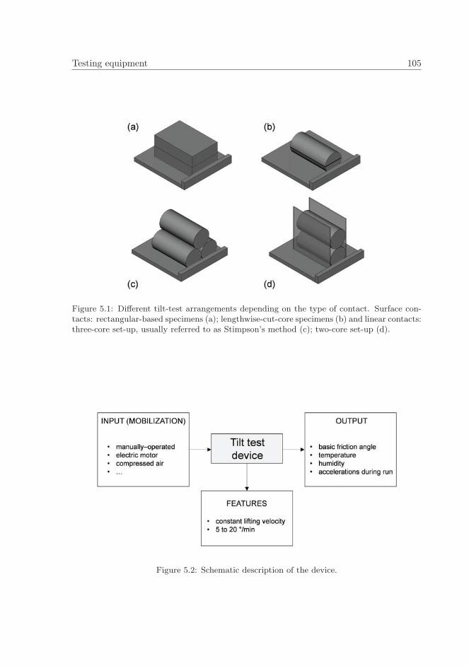
Testing equipment 105
Figure 5.1: Different tilt-test arrangements depending on the type of contact. Surface con-tacts: rectangular-based specimens (a); lengthwise-cut-core specimens (b) and linear contacts:three-core set-up, usually referred to as Stimpson’s method (c); two-core set-up (d).
Figure 5.2: Schematic description of the device.
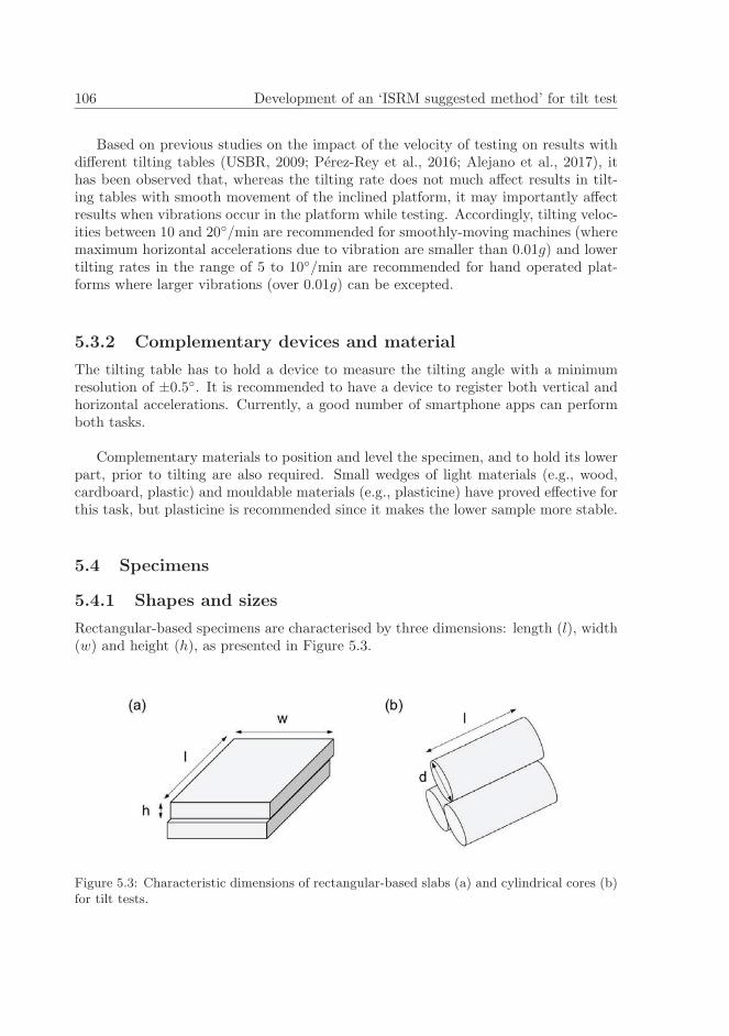
106 Development of an ‘ISRM suggested method’ for tilt test
Based on previous studies on the impact of the velocity of testing on results withdifferent tilting tables (USBR, 2009; Perez-Rey et al., 2016; Alejano et al., 2017), ithas been observed that, whereas the tilting rate does not much affect results in tilt-ing tables with smooth movement of the inclined platform, it may importantly affectresults when vibrations occur in the platform while testing. Accordingly, tilting veloc-ities between 10 and 20◦/min are recommended for smoothly-moving machines (wheremaximum horizontal accelerations due to vibration are smaller than 0.01g) and lowertilting rates in the range of 5 to 10◦/min are recommended for hand operated plat-forms where larger vibrations (over 0.01g) can be excepted.
5.3.2 Complementary devices and material
The tilting table has to hold a device to measure the tilting angle with a minimumresolution of ±0.5◦. It is recommended to have a device to register both vertical andhorizontal accelerations. Currently, a good number of smartphone apps can performboth tasks.
Complementary materials to position and level the specimen, and to hold its lowerpart, prior to tilting are also required. Small wedges of light materials (e.g., wood,cardboard, plastic) and mouldable materials (e.g., plasticine) have proved effective forthis task, but plasticine is recommended since it makes the lower sample more stable.
5.4 Specimens
5.4.1 Shapes and sizes
Rectangular-based specimens are characterised by three dimensions: length (l), width(w) and height (h), as presented in Figure 5.3.
Figure 5.3: Characteristic dimensions of rectangular-based slabs (a) and cylindrical cores (b)for tilt tests.

Specimen preparation 107
Concerning the top sample, the length-to-height ratio (l/h) of this type of speci-mens must be greater than 6, and h/w should be greater than 4, and contact surfaces(l×w) have to be greater than 50 cm2 and specimen width (w) should be larger than10 times the rock grain size, with a minimum of 50 mm.
Rock cores can be used to prepare lengthwise-cut core specimens. This type ofgeometry is similar to rectangular-based specimens. Rock cores should have a diame-ter equal to or greater than 50 mm, and they should have a length-to-diameter ratiol/d ≥ 3.
Rock cores drilled by means of impregnated diamond drill bits, either in the labo-ratory or in the field, can be used to prepare specimens for linear contact tests. Thesespecimens should have a length-to-diameter ratio of 3 or larger. Rock cores of atleast 50 mm diameter are preferred, in order to avoid deficient contact associated toirregularities in the core surface, which tend to be more relevant in smaller specimens.Because of the possibility of polishing’ in the case of worn core bits and/or extremelyhard rock, a quick sand-blasting of the surfaces should be performed, as also in thecase of diamond sawn surfaces. It is important to expose the mineralogy, rather thanwork-hardened (polished) versions (Barton and Choubey, 1977).
5.5 Specimen preparation
The specimens and testing surfaces for rectangular slabs and lengthwise-cut cores haveto be obtained using a circular sawing machine. Recommended saw blades for obtain-ing rock specimens should present teeth or rim grits on the range of 60–100 US Meshand tooth diamond counts within 0.6 to 0.8 carat/cm3. Additionally, the saw bladeshould have a diameter large enough to cut the testing surface with a single operation.The relative speed of the block against the saw blade should be as constant as possible.
Planarity of the surface to be tested can be visually checked and further controlledusing more elaborate means (e.g., roughness profilometer, surface scanner). Smooth-ness of the surface and the occurrence of grooves resulting from cutting should also beexamined, and consequently, non-planar and rough surfaces should be discarded.
Ordinary impregnated diamond drill bits are acceptable to core the rocks in placeor at the laboratory. Similar characteristics as those recommended for saw blades(teeth/rim grits on the range of 60–100 US Mesh and tooth diamond counts within0.6 to 0.8 carat/cm3) can be applied. Cores with irregular surfaces associated todrilling, for instance diameter changes, coarse grooves or indentations, should be dis-carded.

108 Development of an ‘ISRM suggested method’ for tilt test
5.6 Testing procedure
Each test encompasses various repetitions of the following tilting sequence.:
1. The lower part of the specimen(s) is fixed to the tilting platform and the hori-zontality of the surface or contacts have to be assured by means of a spirit-levelor electronic level.
2. Before each tilt-test repetition (5 tests are recommended on each sample) thesurface must be cleaned and rock powder must be removed using a soft paintbrush.
3. The upper part of the specimen has to be placed on top of the other piece(s)with their correspondent surfaces in contact and the relative position of all piecesof the specimen has to be verified, in order to be reproduced in subsequentrepetitions. The sliding direction should be along the maximum dimension ofthe specimen (l).
4. Register the angle of the tilting table at the start of the sliding-movement witha minimum accuracy of 0.5◦.
5. Temperature (◦C) and relative air humidity (%) are recorded during repetitions.
6. A constant fixed rotational-velocity, selected from the interval of 5 to 20/min, isused for tilting the specimens until the upper one starts to slide. At this point,the process is stopped.
7. Maximum sliding distance should not exceed 10% of the maximum length of thespecimen (l), as shown in Figure 5.4, aiming to minimize the wear or polishingof the contact surface.
8. Record the tilt angle βas the difference between the angle when first sliding andthe angle at the horizontal position.
It is recommended to conduct 5 repetitions on each contact surface and to use themedian to obtain a final result. The median is recommended instead of the mean oraverage to avoid errors associated with the occurrence of outliers.
Figure 5.4: Scheme to limit the sliding of the upper part of the specimen

Calculations 109
5.7 Calculations
5.7.1 Rock surfaces (surface contact)
For rock surfaces, the basic friction angle (φb) shall be the calculated as the medianvalue of the 5 repetitions performed (Equation 5.1):
φb = median βi=1,...,5 (5.1)
If more than five repetitions are performed, change the equation accordingly.
5.7.2 Rock cores (linear contact)
For three-core contacts, the basic friction angle (φb) shall be calculated using Equation5.2, as the median value of the tilt angles of the five repetitions performed:
φb = median[tan−1
(√32 tanβi=1,...,5
)](5.2)
If more than five repetitions are performed, change the equation accordingly.
5.8 Reporting of results
The report containing results of a particular tilt testing programme should include thefollowing information:
(a) Lithological description of tested rock(s).
(b) At least, one photograph of the specimens involved in each test; name/identificationof testing surfaces should be clearly shown in the photograph.
(c) Source of the specimens: geographic location of the rock formation, date ofcutting from original rock blocks and storage conditions (temperature (◦C), hu-midity (%)).
(d) For rock-core specimens: project no., borehole no. and depth of specimen fromborehole collar.
(e) Characteristics of saw blade used for cutting the specimens: this section shouldinclude blade diameter, tooth/rim width, grit size and diamond count (andwhether sand blasting was used to reduce/remove ‘polishing’).
(f) Number of specimens tested.

110 Development of an ‘ISRM suggested method’ for tilt test
(g) Dimensions of all specimens —length, width, height and diameter (for rock core).These values should be measured with a device (a caliper gauge is recommended)allowing a resolution of at least 1 mm. Three measurements have to be performedof the three dimensions.
(h) Tilting rate selected for performing all tests.
(i) Date of testing.
(j) Results from tests (φb), including all repetitions (βi) (suggested example can befound at the end of this chapter (Table 5.1).
5.9 Notes and recommendations
Tilt tests replicate small-scale basic principles of sliding behaviour, regarding the defi-nition of friction angle, such as the angle of repose, and they reproduce the conditionsof sliding rock blocks on slopes. However, it has been recognized that adhesion andinterlocking of microscopic roughness may influence the results from tilt tests con-tributing to their non-reproducibility and excessive variability (Hencher and Richards,2015). Results from a benchmark experiment suggest that tilt tests show a reasonabledegree of reproducibility when tilt testing under controlled conditions (Alejano et al.,2017).
Surface finishing (’polishing’) and wear, tilting velocity and equipment vibration,relative humidity and adhesion are some issues that may affect the results of tilt tests.In this section, several notes and recommendations are given, in order to minimize theimpact of these potential problems.
Surface finishing is strongly influenced by the rock minerals, grain size and hard-ness, by the saw blades or disks and the cutting equipment, and particularly by theexpertise of the personnel. Though this SM recommends a particular type of sawblade, planarity and smoothness of the final surfaces can be achieved with differenttools and careful cutting.
So, examining planarity of the rock surfaces is important, and for this purpose therock surface should be positioned on top of a flat surface and the contact inspectedagainst a light source. If a perfect contact is not seen (Figure 5.5), the surface shouldbe discarded.
Surface wear resulting from successive repetitions may yield unreliable results.Small hard debris may cause rolling sliding and decrease the tilt angle, while very finerock powder resulting from surface milling or hard rock polishing may increase the tiltangle. Thus, cleaning of the surfaces prior to all repetitions is essential. This ratherplain task should be carefully performed using such a brusher that neither damagethe rock surface nor leave brusher materials on the surface. Soft tissues are also notrecommended as cleaning materials since they may leave small threads on the surfaces.In any case, limiting sliding of the upper part of the specimen to 10% of the contact

Notes and recommendations 111
length (Figure 5.4) ensures less variable and more representative results. It may benoted that the normal stress acting when sliding occurs is likely to be less than 0.01MPa if the sample dimension (h) is limited to a few centimetres.
Figure 5.5: Detailed view of bad matching observed between two specimens representingundesirable cutting.
According to recent studies (Jang et al., 2018), scale-effect has been reported tohave negligible influence on tilt-test results at a laboratory scale (specimen lengthsranging from 10 to 20 cm-length and l/h ratios greater than 3). A minimum contactsurface (50 cm2) had been stablished as a lower limit (Alejano et al., 2012a) to avoidpoor contact of surfaces. Along these lines, setting a minimum surface better assuresa completely compressive-stress distribution on the contact surface when carrying outthe tilt test.
It has been established that the angular velocity does not affect the results oftilt tests conducted under mechanically controlled conditions (Perez-Rey et al., 2016).However, results may be significantly affected when manually-operated tilting plat-forms are used due to vibrations associated with an imperfectly controlled testing pro-cedure or to mismatching in the mechanical tilting system. So, for manually-operatedtilting tables, a low tilting velocity between 5 and 10◦/min should be used to controlacceleration and ensure comparable results.
Vibrations of the tilting equipment may also influence the results of tilt tests (Ale-jano et al., 2017). It is recommended to use common portable measuring devices todetermine maximum vibrations of the equipment. Values below 0.005g can be consid-ered negligible. Nevertheless, hand-operated 1:100 or 1:200 reduction-gear tilt-tablesare largely without vibration since the rotating mechanism weighs many kg. A concretelaboratory floor area, and heavy and stable benches/tables are a logical assumptionin this regard.

112 Development of an ‘ISRM suggested method’ for tilt test
It is a proven fact that moisture activates adhesion between two slickensided rocksurfaces (Mehrishal et al., 2016, 2017). Since it is not fully recognized if relative hu-midity influences the results of tilt tests, it is recommended to perform the tests underenvironmentally stable conditions (e.g., relative humidity between 50 and 55% andtemperature around 20◦ ± 2◦).
Recent studies by (Li et al., 2017) revealed a small mean difference (2◦) betweenresults from tilt tests using three core linear contacts and surface contacts (Figure5.6). Such differences between the different types of tests require further research andadequate recognition by practitioners that utilize the values of tilt tests to determinethe basic friction angle. In the three-core test, it is important to maintain a tight con-tact between the two lower cores. The upper core will eventually get wedged if the twolower cores are allowed to separate. Two-core tests with loose vertical guiding wallsare recommended in preference to three-core tests. The core axes in both two-coreand three-core tests must be parallel to the dip direction of the tilt table. A deviationof the core axes would lead to an increase in the measured friction angle.
Figure 5.6: Friction angles measured on three-core linear contact specimens (φ3C) and onlengthwise-cut-core (surface contact) specimens (φ3C).
In tests with cores in hard rocks, grooves or irregular profiles are sometimes ob-served on the core surfaces due to poor drilling. In these cases, quick sand-blastinghas shown to produce more reliable results. One of the aims of this suggested methodis to provide guidelines to avoid the common mistakes made when carrying out thesesimple tests without due care. Although the test is apparently a very simple one, itmay involve various physical phenomena associated with the behaviour of the con-tact surfaces, which may result in complex sliding results. The tilt test results may

Conclusions of this chapter 113
be associated not only with frictional but also with adhesion and textural (micro-roughness) phenomena under particular circumstances (Mehrishal et al., 2017; Hencherand Richards, 2015; Aydan et al., 1995). Therefore, a cautious application of the basicfriction angle values obtained is recommended.
Table 5.1: Suggested table for reporting basic friction angle results obtained from tilt tests.
Test arrangement: choose between the following: surface contact, linear contact betweentwo cores or linear contact between three cores.
Date: Tilting rate (◦/min):
Rock type: Specimen identification:
Series β1 β2 β3 β4 β5 T W φba
(◦) (◦) (◦) (◦) (◦) (◦C) (%) (◦)Series 1Series 2. . .Series iaEstimated using Equation 5.1 in the case of surface contact and linear contact betweentwo cores, or using Equation 5.2 for linear contact between three cores.
5.10 Conclusions of this chapter
An ‘ISRM Suggested Method for Determining the Basic Friction Angle of Planar RockSurfaces by Means of Tilt Tests’ was proposed. The aim of this suggested procedureis to avoid errors in tilt-tests performance and in the interpretation of results, by pro-viding a basis for further amendments in the future.
For some time now, the ISRM has been publishing on its website, for educationalpurposes, some representative videos of the Suggested Methods with detailed expla-nations on how to proceed to carry out different types of common laboratory tests,such as the determination of the shear strength of rock joints or a basic rock samplepreparation.
Aiming at contributing to this initiative, the author of this PhD dissertation —to-gether with two lab-colleagues and under the scientific guidance of the supervisor ofthis PhD thesis—have developed a video where the procedure for the estimation of thebasic friction angle of a planar rock surfaces, as presented in this chapter, is described.The video was approved by the ISRM Commission on Testing Methods and it can beaccessed from the ISRM website (https://www.isrm.net/gca/?id=1233).

114 Development of an ‘ISRM suggested method’ for tilt test
Chapter 6
Implications of the basicfriction angle in a case study
In the core of a a case study devoted to assess the stability against sliding andtoppling mechanisms of a paradigmatic granitic boulder (Pena do Equilibrio boulder)located in the SW of Galicia (NW Spain), the relevance of a realistic estimation of thebasic friction angle through the methodology developed within this PhD thesis is broughtto light in the present chapter. The present chapter has been submitted for publicationto the International Journal of Rock Mechanics and Mining Sciences:
• Perez-Rey, I., Alejano, L. R., Riquelme, A., and Gonzalez-deSantos, L. (2019).Failure mechanisms and stability analyses of granitic boulders focusing a casestudy in Galicia (Spain) [Submitted for publication]. International Journal ofRock Mechanics and Mining Sciences
Some comments regarding other studies in which the author has participated and wherethe basic friction angle has relevance are briefly presented at the end of this chapter.
6.1 Introduction
Large granite boulders are distinctive geomorphological elements or structures usuallyfound in mountain or abrupt granitic humid areas. A large amount of rainfall con-tributes to the processes eventually leading to the formation of these boulders, so theytend to be more common in wet temperate climates. Therefore, these granite bouldersare common all over the world but particularly in regions such as northern Spain (Ale-jano et al., 2010; Ayala-Carcedo et al., 2003), Portugal (Vidal-Romanı, 1989; Migonand Vieira, 2014), Italy (Pera and Sorriso-Valvo, 2000), Turkey (Aydin, 2006), USA(Tolman and Robertson, 1969; Fisher, 2004; Chapin et al., 2014), Southern Australia(Twidale, 1982, 1989), Brazil (Valeriano and Magalhaes, 1984), Hong-Kong (GEO,2017) or Malaysia (Md Dan et al., 2015).
115

116 Implications of the basic friction angle in a case study
Occasionally, the instability of these boulders represent a potential risk for peopleor infrastructures (Alejano et al., 2010; Christianson et al., 1995).
These boulders are formed through evolving spheroidal weathering (Ollier, 1971;Migon, 2006) so they tend to present roughly spheroidal or ellipsoidal shape, but inpractice they often show surface irregularities associated with the heterogeneous na-ture of granitic rock and with the occurrence of pre-existing rock mass discontinuitiesthat partially control their formation.
Traditional rock slope engineering studies (Hoek and Bray, 1974; Wyllie and Mah,2004) developed methodologies for analysing the stability of geometrical shaped rockblocks delimited by pre-existing planar discontinuities, such as rock slabs, prisms,wedges or columns. These potentially unstable blocks tend to form when excavatingengineered slopes or rock cuts. Stability against sliding or toppling of individual orsets of these elements can be quantified according to these approaches.
However, methodologies to estimate the stability of naturally occurring graniteboulders of irregular shape have not been developed so far, something the authorsattribute to two facts. Firstly, rarely does the stability of boulders involve a hazardfor people or infrastructures; secondly, the complex geometry of these boulders wasdifficult to measure and their stability cannot be easily quantified according to existingapproaches.
Nevertheless, some studies on the stability of individual or sets of boulders can befound in literature. In this way, Christianson et al. (1995) analysed the stability ofsome Buddha carvings in granite boulders in Japan accounting for potential seismictriggering effects; Alejano et al. (2010) presented a stability analysis of a boulder ina study that partially motivated the development of the current work. The stabilityagainst toppling of rock slabs with rounded corners has been studied, first, in an indi-vidual basis (Alejano et al., 2015) and then for the case of a number of interacting rockslabs in line with the block toppling stability analysis proposed by Goodman and Bray(1976), for the case of sharp-edge and rounded-edge blocks (Alejano et al., 2018b), astudy co-written by the author of this dissertation.
Undoubtedly, a typical granite boulder is nothing but a cubic or slab-shaped ratherirregular granite block subjected to spheroidal weathering. So the approaches devel-oped in the mentioned publications have also served as an input for the developmentof the present study.
Even though the actual majority of these boulders is not usually hazardous, incase the block is located in a cliff or a natural slope it may fall down. This potentialrockfall of unstable boulders has shown to cause accidents and being of concern in acertain number of places (de Almeida and Kullberg, 2011; Topal et al., 2012). In thissense, it is interesting to develop approaches to quantify its stability. Additionally,analysing the stability of granitic boulders could contribute to a better understandingof geodynamical evolution, not only for granitic but also for other rock masses.

Geomorphological context 117
Based on these two mentioned reasons, it has been considered of interest to developa rock mechanics approach to quantify boulder stability. Within this framework, astability study of a paradigmatic granitic boulder —Pena do Equilibrio (’equilibriumstone’)—located in Galicia (NW Spain) is proposed. To do that, it has been first re-sorted to advanced surveying techniques in order to obtain a detailed geometry of theboulder, and to rock characterisation methods to estimate the friction of the rock con-tact surface. Then, and based on physical modelling of engineered small-size blocks,techniques to estimate factors of safety against sliding and toppling for different shapesand positions of irregular blocks have been reviewed. Finally, physical models and cal-culations have been extended to quantify the stability of the granitic boulder underscrutiny, and the obtained results made sense in relation to actual stability observa-tions, also agreeing reasonably well with a 3D-printed physical model of the boulder.
The presented approach can be extended or adapted to quantify the stability ofother cases involving irregularly-shaped granitic boulders.
6.2 Geomorphological context
Boulders can be considered one of the most common and characteristic landforms ofgranitic terrains (Twidale and Vidal-Romanı, 2005). Their origin can be encounteredwithin the typical weathering sequence of granitic rock masses, a process described byDurgin (1977), in which four typical stages can be recognised: fresh rock, corestones,decomposed granitoid and saprolite. The development of these structures is dominatedby the mechanism of spheroidal weathering, a chemical process that mainly affects uni-form, well-jointed rocks like granite, dolerite or basalt, but also other lithologies suchas gabbros and sandstones (Ollier, 1971).
The process of boulder formation is developed in two stages: first, subsurfacedifferential-weathering acts on the granitic rock mass being complemented afterwardswith erosive events (wind, rainfall), which develop the eventual excavation of the core-stone to form a boulder (Figure 6.1). Subsurface weathering principally alters micasand feldspars to produce clays, with the intervention of different chemical processessuch as solution, alteration and hydrolysis (Twidale and Vidal-Romanı, 2005).
Weathering of granitic batholiths presents joint-controlled geomorphic features,which means that it is clearly dependent on the rock mass structure, particularly ontheir main joint sets, usually displayed orthogonally. Fracturing spacing is consideredthe main factor affecting maximum size and shape of boulders, whereas roundness andthe actual size depend on the duration and intensity of subsurface weathering (Migon,2006).
In general terms, boulders appear in different shapes, from almost perfect spheresto ellipsoidal bodies and even slender slabs, depending not only on the weatheringdegree to which they were subjected, but also on the geometrical variability of thejoint sets affecting the granitic rock mass. Migon (2006) has related the presence of
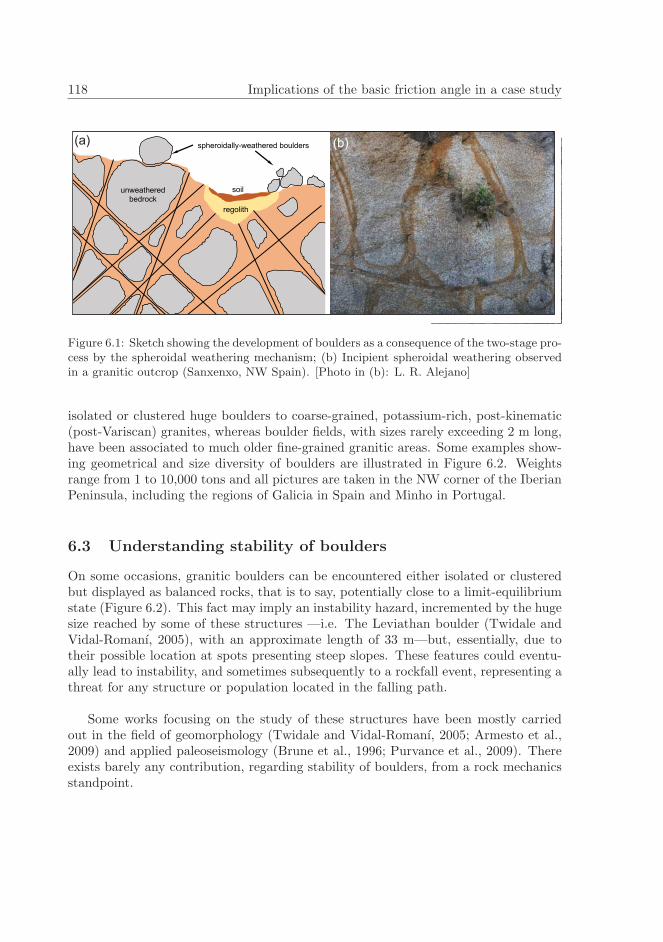
118 Implications of the basic friction angle in a case study
Figure 6.1: Sketch showing the development of boulders as a consequence of the two-stage pro-cess by the spheroidal weathering mechanism; (b) Incipient spheroidal weathering observedin a granitic outcrop (Sanxenxo, NW Spain). [Photo in (b): L. R. Alejano]
isolated or clustered huge boulders to coarse-grained, potassium-rich, post-kinematic(post-Variscan) granites, whereas boulder fields, with sizes rarely exceeding 2 m long,have been associated to much older fine-grained granitic areas. Some examples show-ing geometrical and size diversity of boulders are illustrated in Figure 6.2. Weightsrange from 1 to 10,000 tons and all pictures are taken in the NW corner of the IberianPeninsula, including the regions of Galicia in Spain and Minho in Portugal.
6.3 Understanding stability of boulders
On some occasions, granitic boulders can be encountered either isolated or clusteredbut displayed as balanced rocks, that is to say, potentially close to a limit-equilibriumstate (Figure 6.2). This fact may imply an instability hazard, incremented by the hugesize reached by some of these structures —i.e. The Leviathan boulder (Twidale andVidal-Romanı, 2005), with an approximate length of 33 m—but, essentially, due totheir possible location at spots presenting steep slopes. These features could eventu-ally lead to instability, and sometimes subsequently to a rockfall event, representing athreat for any structure or population located in the falling path.
Some works focusing on the study of these structures have been mostly carriedout in the field of geomorphology (Twidale and Vidal-Romanı, 2005; Armesto et al.,2009) and applied paleoseismology (Brune et al., 1996; Purvance et al., 2009). Thereexists barely any contribution, regarding stability of boulders, from a rock mechanicsstandpoint.

Understanding stability of boulders 119
Figure 6.2: Different examples of granitic boulders in the NW Iberian peninsula: (a) ellip-soidal boulder still surrounded by highly decomposed granite; (b) quasi-spherical boulderrecently released from completely decomposed granite; (c) boulder presenting a sub-verticalcrack; (d) ellipsoidal ‘rocking stone’, something attributed to a concave base; (e) twin boul-ders; (f) large boulder probably fallen down from a close mountain; (g) very large boulder(10,000 tons) in a mountain peak and (g) slab-like rounded cornered blocks. Location ofevery boulder written below every picture and approximate scale reflected.
Moreover, some of these studies have focused on the stability of slender blocks(Alejano et al., 2015; Purvance, 2009), some of them from a rock slope engineeringperspective and mainly revisiting toppling mechanisms (Alejano et al., 2018b; Liuet al., 2010; Bobet, 1999; Yagoda-Biran and Hatzor, 2013).
Other authors have analyzed the maximum boulder size forming in overhangingcliffs associated to tensile failure and the occurrence of earthquakes, but the failuremechanisms analyzed differed from the case of rounded granite boulders under studyhere (Katz et al., 2011; Siman-Tov et al., 2017). Due to all these particularities, ithas been considered important to provide tools for correctly assessing the stability ofpotentially unstable boulders.
In the heart of this case study, it has been observed that the main instability mech-anisms affecting boulders lying on slopes —sliding and toppling—could be relevantlyaffected by some geometrical features, like the actual shape of the boulder, mass dis-tribution and the type of contact between the boulder and the resting surface. In thisline, some approaches, by means of simple engineered rock and 3D printed elements,have been carried out aiming to understand the effect of these factors on block sta-bility. These analyses also served to develop a realistic approach for estimating thestability state of a balanced granitic boulder.

120 Implications of the basic friction angle in a case study
6.4 Laboratory physical modelling of simple geometric models
With the aim of studying the stability of the Pena do Equilibrio boulder, it was con-sidered relevant to review first the traditional procedure for estimating safety factor,particularly for toppling failure (considering gravity as the unique driving force), inorder to be applied later to the boulder under scrutiny. To test the analytical approachand analyse factors at stake, some rock models with symmetric and asymmetric sec-tions were selected and engineered in laboratory by cutting and assembling smallergranitic pieces (Figure 6.3a-f). The advantage of these physical models resides in theirsimple basic geometry, which allows a simple analytical estimation of the angle of top-pling for each specimen. Additionally, it is possible to carry out simple tilt tests undercontrolled environmental conditions and constant lifting velocities (12 ◦/min) by usingthe tilting table partially developed in this doctoral thesis and, thus, analysing in anexperimental manner, the analytically predicted angles (against of toppling or sliding).
The stability against sliding is controlled by the plane dip (β) and the basic frictionangle of the used granite (Equation 6.1) which was found to be 31.2◦ in a large seriesof tilt tests (Alejano et al., 2017).
FoSs =tanφb
tanβ(6.1)
The basic equation controlling the stability against toppling of a rigid block ispresented in Equation 6.2 and it can be used to estimate the factor of safety, andsubsequently, the stability of a block against toppling. This simple equation just con-siders the ratio of the stabilizing and overturning moments, which in the simplest casewhere the only driving force is the weight of the specimen can be computed accordingto the forces acting along x and y-axes, in relation to a rotation axis located in thelower corner of the block in the direction of tilting.
FoSt =
∑Mstabilizing∑Moverturning
(6.2)
The forces involved in the analysis of each specimen result only from its own weightand they are applied at the centres of gravity of the specimens, in the case of sym-metric specimens (Figure 6.3(d, e, g)) or at the centres of gravity of subsections, inthe case of the rest of asymmetric figures (Figure 6.3).
The most prone mechanism, sliding or toppling, will be the one theoretically oc-curring at a lower tilting angle.

Laboratory physical modelling of simple geometric models 121
Figure 6.3: (a)-(g) Rock specimens used for the experimental program to review safety factorequation; (h) Sketch of the specimens used for the experimental determination of the angle oftoppling; (i) Sketch of the subdivision of one specimen for estimating factor of safety againsttoppling, including the location of the centres of gravity of its parts.
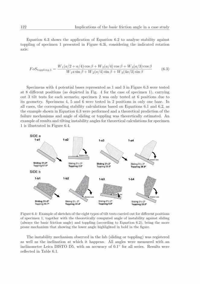
122 Implications of the basic friction angle in a case study
Equation 6.3 shows the application of Equation 6.2 to analyse stability againsttoppling of specimen 1 presented in Figure 6.3i, considering the indicated rotationaxis.
FoStoppling,1 =W 1(a/2 + a/4) cosβ +W 2(a/4) cosβ +W 3(a/3) cosβ
W 1a sinβ +W 2(a/4) sinβ +W 3(4a/3) sinβ(6.3)
Specimens with 4 potential bases represented as 1 and 3 in Figure 6.3 were testedat 8 different positions (as depicted in Fig. 4 for the case of specimen 1), carryingout 3 tilt tests for each scenario; specimen 2 was only tested at 6 positions due toits geometry. Specimens 4, 5 and 6 were tested in 2 positions in only one base. Inall cases, the corresponding stability calculations based on Equations 6.1 and 6.2, asthe example shown in Equation 6.3 were performed and a theoretical prediction of thefailure mechanisms and angle of sliding or toppling was theoretically estimated. Anexample of results and tilting instability angles for theoretical calculations for specimen1 is illustrated in Figure 6.4.
Figure 6.4: Example of sketches of the eight types of tilt tests carried out for different positionsof specimen 1, together with the theoretically computed angle of instability against sliding(always the basic friction angle) and toppling (according to Equation 6.2), being the moreprone mechanism that showing the lower angle highlighted in bold in the figure.
The instability mechanism observed in the lab (sliding or toppling) was registeredas well as the inclination at which it happens. All angles were measured with aninclinometer Leica DISTO D5, with an accuracy of 0.1◦ for all series. Results werereflected in Table 6.1.
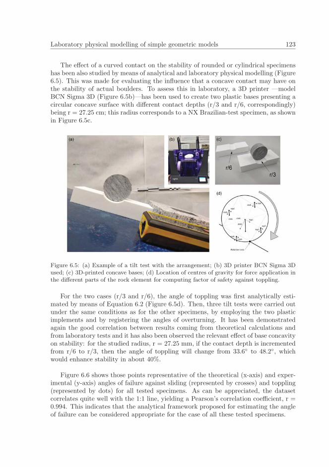
Laboratory physical modelling of simple geometric models 123
The effect of a curved contact on the stability of rounded or cylindrical specimenshas been also studied by means of analytical and laboratory physical modelling (Figure6.5). This was made for evaluating the influence that a concave contact may have onthe stability of actual boulders. To assess this in laboratory, a 3D printer —modelBCN Sigma 3D (Figure 6.5b)—has been used to create two plastic bases presenting acircular concave surface with different contact depths (r/3 and r/6, correspondingly)being r = 27.25 cm; this radius corresponds to a NX Brazilian-test specimen, as shownin Figure 6.5c.
Figure 6.5: (a) Example of a tilt test with the arrangement; (b) 3D printer BCN Sigma 3Dused; (c) 3D-printed concave bases; (d) Location of centres of gravity for force application inthe different parts of the rock element for computing factor of safety against toppling.
For the two cases (r/3 and r/6), the angle of toppling was first analytically esti-mated by means of Equation 6.2 (Figure 6.5d). Then, three tilt tests were carried outunder the same conditions as for the other specimens, by employing the two plasticimplements and by registering the angles of overturning. It has been demonstratedagain the good correlation between results coming from theoretical calculations andfrom laboratory tests and it has also been observed the relevant effect of base concavityon stability: for the studied radius, r = 27.25 mm, if the contact depth is incrementedfrom r/6 to r/3, then the angle of toppling will change from 33.6◦ to 48.2◦, whichwould enhance stability in about 40%.
Figure 6.6 shows those points representative of the theoretical (x-axis) and exper-imental (y-axis) angles of failure against sliding (represented by crosses) and toppling(represented by dots) for all tested specimens. As can be appreciated, the datasetcorrelates quite well with the 1:1 line, yielding a Pearson’s correlation coefficient, r =0.994. This indicates that the analytical framework proposed for estimating the angleof failure can be considered appropriate for the case of all these tested specimens.

124 Implications of the basic friction angle in a case study
Figure 6.6: Comparison of the experimental (x-axis) and theoretical (y-axis) angle of sliding(crosses) and toppling (dots) for all tested specimens.
All results obtained from tilt tests together with those estimated through the ap-plication of Equations 6.1 and 6.2 are presented in Table 6.1 for all specimens andtesting positions. In this table, error is simply the difference between analytical andexperimental angles. It is relevant to remark that the average value of errors from allresults in Table 6.1 is −0.3◦ with a standard deviation of 1.3◦, an indication that forcontrolled geometry and surface strength the stability computing capacity is ratheraccurate. However, it should be pointed out that all these specimens have a constantgranite thickness (they have a vertical symmetry plane, containing their gravity cen-tre, whose projection for the horizontal position falls in the centre of the base) and fortilting they are positioned with the symmetry plane normal to the strike of the tiltingsurface. This makes calculations simpler. For the case of irregular boulders resting onrock planes, this may not always be the case, so stability computations may not bethat straightforward.
To study this scenario in laboratory, it was carried out a tilt test involving twocylindrical specimens with same radius, r = 27 mm (one made up of a gneiss withapproximate density γr = 2700 kg/m3 measuring 100 mm-height and the other onemade up of steel, with approximate density γs = 7800 kg/m3 and measuring 35 mm-height). This test consisted in placing the two specimens in the way shown by Figure6.7, that is with the top piece moved outwards a distance r/2. This position of thetop steel specimen distances the centre of gravity out of the plane of symmetry ofthe lower specimen, as can be appreciated in the front view Figure 6.7. Then, the

Laboratory physical modelling of simple geometric models 125
specimen was progressively tilted until toppling of the entire set occurred, when thetilting angle was registered. The experiment was also repeated with both specimensaligned by their vertical axis.
Table 6.1: Experimental (βi) and theoretical (βtheo.) instability tilt angle for all specimens withdifferent positions tilted in laboratory until sliding (S) or toppling (T) failure occurs. The differentpositions are illustrated in Figure 6.3 for specimen 1 and explained in the text. βtopp. is the angletheoretically computed for toppling instability. βtheo. is the lower value between βtopp. and frictionangle (31 ± 2◦), theoretically indicating the angle at which instability is expected. βmean is theaverage of the observed experimental tilt tests (β1, β2 and β3). Error refers to the difference betweenthe mean experimental angle observed (βmean) and the theoretical angle expected (βtheo.).
Specimen Position βtopp. βtheo. S/T β1 β2 β3 βmean error
1 a1 67.5 31±2 S 33.7 30.2 29.6 31.2 0.2a2 2.5 2.5 T 3.5 3.3 3.3 3.4 0.9a3 58.8 31±2 S 34.8 30.6 27.3 30.9 -0.1a4 26.6 26.6 T 27.4 27.2 26.3 27.0 -0.4b1 56.7 31±2 S 33.0 31.5 28.0 30.8 -0.2b2 31.4 31±2 T 30.9 30.4 30.4 30.6 -0.4b3 9.9 9.9 T 10.8 10.4 10.2 10.5 0.6b4 22.5 22.5 T 22.9 23.1 23.0 23.0 0.5
2 a1 57.5 31±2 S 32.8 25.3 27.3 28.5 -2.5a2 45.0 31±2 S 34.2 31.2 30.6 32.0 1.0a3 28.4 28.4 T 27.8 27.8 27.7 27.8 -0.6b1 61.7 31±2 S 34.6 26.8 27.1 29.5 -1.5b2 32.6 31±2 S 32.3 32.1 32.1 32.2 1.2b3 20.8 20.8 T 22.7 22.1 22.3 22.4 1.6
3 a1 66.0 31±2 S 33.5 30.9 27.0 30.5 -0.5a2 1.4 1.4 T 2.60 2.70 2.70 2.70 1.3a3 61.4 31±2 S 29.0 25.6 26.5 27.0 -4.0a4 < 0 — — — — — — —b1 45.0 31±2 S 30.4 27.2 30.1 29.2 -1.8b2 24.5 24.5 T 25.4 25.3 25.6 25.4 0.9b3 4.0 4.0 T 3.20 3.20 3.10 3.20 -0.8b4 28.6 28.6 T 29.1 29.0 29.2 29.1 0.5
4 a1 20.0 20.0 T 20.2 20.3 20.5 20.3 0.3a2 20.0 20.0 T 21.6 21.8 21.8 21.7 1.7
5 a1 16.1 16.1 T 15.6 15.6 15.5 15.6 -0.5a2 16.1 16.1 T 15.7 15.7 15.8 15.7 -0.4
6 a1 1.80 1.80 T 3.90 4.10 3.80 3.90 2.1a2 26.8 26.8 T 23.8 23.8 24.2 23.9 -2.9
7 a1 33.6 33.6 T 33.3 32.5 32.8 32.9 -0.7a2 33.6 33.6 T 32.7 32.6 32.6 32.6 -1.0
8 a1 48.2 48.2 T 47.3 48.3 48.4 48.0 -0.2a2 48.2 48.2 T 46.7 47.2 49.0 47.6 -0.6
Set rock + steel Left r/2 17.3 31±2 T 16.5 15.9 16.2 16.2 -1.1Centred 17.8 31±2 T 16.9 16.9 16.5 16.8 -1.0Right r/2 17.3 31±2 T 16.1 15.8 16.4 16.1 -1.2

126 Implications of the basic friction angle in a case study
From the whole experiment, two observations (which may be of relevance whenassessing the stability of real boulders) can be extracted. Firstly, for a given tiltingangle (β) the safety factor is reduced with respect to those configurations which keepthe centre of gravity in a symmetry plane (e.g. tilt test with both specimens aligned);secondly, the rotation point, for the not-aligned set, becomes deviated from the lineof maximum slope, as shown by δ angle in Figure 6.7b.
Based on this test configuration (Figure 6.7a) with the top specimen displaced, itis possible to obtain, first, the factor of safety (Equation 6.4) at any moment in thetilting process and also the slope βcrit. at which the set will be unstable (Equation 6.5).Additionally, in this case, the element does not topple in the direction of maximumslope but in a direction forming an angle δ with this one, which can be computed asproposed by Equation 6.6.
Figure 6.7: (a) Three different views of the set used for this experiment (shown in the photo);(b) evolution of the left view of a tilt test in three positions (initial horizontal position, aftersome tilting and at the critical case) indicating the projection on the tilting plane of the baseof the specimen and that of the centre of gravity of the set. Remark instability occurs whenthe projection of the weight attains the border of the base.
FoSt =Mstab.
Movert.=
W × xG−crit. × cosβ
W × zG sinβ=
xG−crit.
xG=
tanβcrit.
tanβ(6.4)
βcrit. = tan−1
(xG−crit.
zG
)(6.5)
δ = tan−1
(yG
yG−crit.
)(6.6)

Laboratory physical modelling of simple geometric models 127
Some detailed calculations for this test are presented in Figure where from anglesof βcrit. = 17.3◦ and δ = 14.2◦ were obtained, consistent with the results observed inthe tilt tests. The authors have carried out three repetitions of tests for the case ofthe steel piece offset r/2 in both directions and for the case with the sample centred.Results are presented in the last lines of Table 6.1 showing good agreement. The 1◦
difference between the analytical and experimental results can be attributed to a smallrounding in the base of the gneiss specimen. In addition, the fact of not toppling inthe maximum slope direction was observed by justifying the computed δ angle.
6.4.1 Effect of rounding on the stability of boulders
The rounding of block edges and corners represent the evident effect of the spheroidalweathering mechanism affecting rock masses. From an engineering point of view, thiseffect may have relevant influence on the stability of slender rock slabs against top-pling, but also in actual rock slopes prone to fail under this mechanism, as studiedby Alejano et al. (2015, 2018b). The basic influence of a rounded edge associated tothe rotating axis can be quantified according to the equations illustrated in Figure6.8. Readers are referred to the above mentioned references for further analysis. Re-garding the role played by the spheroidal weathering mechanism on the developmentof granitic boulders, the effect of rounding has been found relevant when analysingstability particularly against toppling, but it may also affect sliding slightly.
Figure 6.8: Factor of safety of a single block with sharp edges (a) and rounded edges (b) aspresented by Alejano et al. (2018b).
To gain insight on these effects and based on the presented equations (Figure 6.8),a theoretical 2D rectangular block of length, L and height, H has been analysed interms of stability against toppling failure. The effect of rounding is introduced in thefollowing analysis by a roundness factor, ρ, defined as the percentage, in unit terms,of the half base of the block (L/2), in such a way that ρ = 0 corresponds to a slabwith sharp edges and ρ = 1 a block with completely rounded edges. In this case, it

128 Implications of the basic friction angle in a case study
is possible to create a chart, for different values of the roundness factor and contactplane dip angles, different curves for the factor of safety considering various L/H ratios.
Figure 6.9 shows that sub-vertical ellipsoidal boulders are more prone to instabil-ity than the spheroidal ones and being these spheroidal ones more prone to instabilitythan sub-horizontal ellipsoidal ones. Indicatively, if a value of ρ = 0.5, is taken, whichmeans rounded edges of half of the length of the block, the plump blocks (L/H = 2.7)will be stable when resting on a plane less than 53 dip (around 70◦ for edged blocks),the squared ones (L/H = 1) for less than 27◦ (45◦ for no rounding) and the slenderones (L/H = 0.5) for less than 15◦ (27◦ for no rounding). In conclusion, it is clearthat rounding plays a key role in instability and that this role can be quantified forperfectly-rounded corners.
Figure 6.9: Representative chart for three levels of the factor of safety (1, 1.2 and 1.5) againsttoppling, for increasing rounding of edges (ρ from 0 to 1) and dip angle varying from 0 to60◦.
6.4.2 The case of Pena do Equilibrio boulder
The granitic boulder under scrutiny, locally known as Pena do Equilibrio (‘EquilibriumStone’), is located near the town of Ponteareas in the province of Pontevedra (Gali-cia, NW Spain). Geologically, the rock that forms the boulder has been describedby the Spanish Geological Survey (IGME, 1981) as a fine-to-medium-grained, biotite-amphibole granodiorite. The structure lies over a granitic base, standing some metersabove a road, and forming a sort of granitic plinth, as it can be observed in Figure 6.10.

Laboratory physical modelling of simple geometric models 129
Figure 6.10: General view of the Pena do Equilibrio (‘Equilibrium Stone’).
Some features of this boulder have motivated the assessment of its stability, beingthe obvious one the risk perception. Other particularities are a pseudo-ellipsoidal ge-ometry and rather large dimensions (about 9 m length and 3.7 m height), the positionabove a local road and the natural inclination, β, with which it is displayed respect tothe ground (approximately β = 27◦ dip). Another relevant feature is the small contactarea between the boulder and the base.
6.4.3 3D surveying and geometrical calculations
Regarding the complex shape of the boulder and its small contact area, the first step toperform stability analyses required a painstaking in-situ 3D surveying of the structure.The use of a Terrestrial Laser Scanner (TLR) was successfully applied to determinethe geometry of geological structures by 3D point-cloud acquisition, in particular ofrock boulders (Armesto et al., 2009). This technique was selected to perform the topo-graphical survey of the boulder under study, specifically those parts demanding highaccuracy, like the contact area. To perform this task, a FARO Focus 330X LiDARwas selected. Several scan stations were performed to scan all the boulder surface, andregistered using external targets. A 3D point cloud (3DPC) was generated in a localreference system. All scan stations were levelled, being the vertical axis of the localreference system (z-axis) coincident with the gravity direction. Consequently, dip mea-surements can be directly extracted from the 3DPC. In addition to the external targets,

130 Implications of the basic friction angle in a case study
several targets were placed on the base of the boulder and consequently scanned. Thelocal coordinates of these targets were extracted for further application of the boulderreconstruction. Special attention was paid to the scanning of the boulder-base contact.
Figure 6.11: Different views from the of the boulder under study from aerial photography:West (a), North (b), South (c) and top view (d). Note control points on photos (b) and (c).
The situation and size of the boulder prevented a complete terrestrial scanning,specifically of the upper face. Therefore, the TLS survey was complemented withaerial imagery obtained with a 12 Mpx camera mounted on a Phantom 3 UnmannedAircraft System (UAS). Figure 6.11 shows different aerial photographs, which wereeventually processed and exported as a 3DPC by means of the photogrammetric suitePhotoscan (Agisoft, 2018). The Structure from Motion (SfM) reconstruction processincluded the previously located targets on the base of the boulder. Coordinates ofthese targets were inserted as Ground Control Points (GPC’s) and the SfM recon-struction was registered to the TLS 3DPC (i.e., both 3DPC were defined in the samelocal reference system). Finally, both 3DPC’s were merged into one, providing veryaccurate information of the entire area. Once the complete 3DPC was processed, itwas necessary to isolate the boulder from the general dataset (Figure 6.12a, b), a taskcarried out with the software CloudCompare (Girardeau-Montaut, 2018). The con-tact area was calculated by creating a 3D polyline at the contour corresponding to theintersection between those points of the boulder and those of the lower rock where itrests. The 3D polyline was afterwards projected onto a plane, giving a contact surfaceof approximately 0.61 m2 (Figure 6.12c).
The estimation of volume and centre of mass of the boulder required the generationof a mesh, by using Poisson’s surface reconstruction (Kazhdan et al., 2006), from theSfM-TLS merged 3DPC. This process was carried out with the open software MeshLab

Laboratory physical modelling of simple geometric models 131
Figure 6.12: (a) Realistic view of the 3D point cloud with CloudCompare; (b) isolation of 3Dpoint cloud of the boulder; (c) detail of a horizontal projection (top view) of the 3D pointcloud, including the polyline corresponding to the edge of the contact area.
(Cignoni et al., 2008). For the given mesh, the estimated volume was 142.22 m3 andthe centre of gravity is located at local coordinates x = 7.914 [m], y = –2.851[m], z= 113.036 [m], being z-axes coincident with gravity direction. Table 6.2 summarisessome geometrical parameters of the boulder under study, which were useful to carryout stability analyses against sliding and toppling.
Table 6.2: Geometrical features of the boulder and of the contact plane.
Geometrical parameter Units Value
Volume, V b [m3] 142.22Centre of gravity, (cog) x, y, z coordinates [m] 7.915, –2.854, 113.036Theoretical contact area, A [m2] 0.61Dip direction of the contactplane
[◦] 163
Dip of the contact plane [◦] 27
6.4.4 Geomechanical characterization of the contact
A basic geomechanical characterization was carried out in order to obtain informationregarding parameters needed to quantify stability. This included density and basicrock joint characterization according to the Barton strength criteria. Rock sampleswere collected and cut into slab-like specimens, which were tested for density and forthe basic friction angle (φb). The average density obtained was 2.57 g/cm3, and the
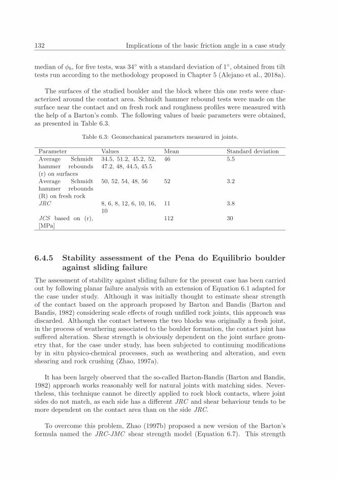
132 Implications of the basic friction angle in a case study
median of φb, for five tests, was 34◦ with a standard deviation of 1◦, obtained from tilt
tests run according to the methodology proposed in Chapter 5 (Alejano et al., 2018a).
The surfaces of the studied boulder and the block where this one rests were char-acterized around the contact area. Schmidt hammer rebound tests were made on thesurface near the contact and on fresh rock and roughness profiles were measured withthe help of a Barton’s comb. The following values of basic parameters were obtained,as presented in Table 6.3.
Table 6.3: Geomechanical parameters measured in joints.
Parameter Values Mean Standard deviation
Average Schmidthammer rebounds(r) on surfaces
34.5, 51.2, 45.2, 52,47.2, 48, 44.5, 45.5
46 5.5
Average Schmidthammer rebounds(R) on fresh rock
50, 52, 54, 48, 56 52 3.2
JRC 8, 6, 8, 12, 6, 10, 16,10
11 3.8
JCS based on (r),[MPa]
112 30
6.4.5 Stability assessment of the Pena do Equilibrio boulderagainst sliding failure
The assessment of stability against sliding failure for the present case has been carriedout by following planar failure analysis with an extension of Equation 6.1 adapted forthe case under study. Although it was initially thought to estimate shear strengthof the contact based on the approach proposed by Barton and Bandis (Barton andBandis, 1982) considering scale effects of rough unfilled rock joints, this approach wasdiscarded. Although the contact between the two blocks was originally a fresh joint,in the process of weathering associated to the boulder formation, the contact joint hassuffered alteration. Shear strength is obviously dependent on the joint surface geom-etry that, for the case under study, has been subjected to continuing modificationsby in situ physico-chemical processes, such as weathering and alteration, and evenshearing and rock crushing (Zhao, 1997a).
It has been largely observed that the so-called Barton-Bandis (Barton and Bandis,1982) approach works reasonably well for natural joints with matching sides. Never-theless, this technique cannot be directly applied to rock block contacts, where jointsides do not match, as each side has a different JRC and shear behaviour tends to bemore dependent on the contact area than on the side JRC.
To overcome this problem, Zhao (1997b) proposed a new version of the Barton’sformula named the JRC-JMC shear strength model (Equation 6.7). This strength
Laboratory physical modelling of simple geometric models 133
criterion takes into account the additional influence of the so-called joint matchingcoefficient (JMC ) a parameter to be estimated based on the matching of the two jointsides.
τ = σn tan
[JRC × JMC × log10
(JCS
σn
)+ φr
](6.7)
This is a variation of the Barton-Bandis formula where the JMC parameter hasto be included. Some studies have shown that this parameter depends on the level ofcontact of the surfaces. Based on an estimation of potential contact of the surface, onprevious experiences developed by the authors on large granite block tilt testing46 andon the recommendation by Zhao (1997b) the JMC should be equalled to 0.3; whenany value lower than this is estimated, JMC was set to this value (JMC=0.3) for thestudied contact.
In order to compute stability, first, the weight of the boulder (Wb) was estimated.Based on the volume recovered from the 3D point cloud (Table 6.2) and consideringthe average specific weight of the rock, γrock = 25.7 kN/m3, the weight of the boulderwas estimated in 3655 kN. Therefore, theoretical normal and shear stresses exerted bythe boulder at the contact plane, as depicted in Figure 6.13, for a dip angle β= 27◦,become (Equations 6.8 and 6.9):
σn,b =W b cosβ
A= 5.34 [MPa] (6.8)
τ b =W b sinβ
A= 2.72 [MPa] (6.9)
Shear strength, τa , available at the contact was computed by means of Equation6.7, considering the following in-situ estimative inputs for the equation:
• Basic friction angle, φb = 34◦
• Number of Schimdt-hammer rebounds for the contact plane, r = 46, so JCS =112 MPa
• Number of Schmidt-hammer rebounds for a fresh rock surface, R = 52
• Joint Matching Coefficient, JMC = 0.3
• Joint Roughness Coefficient, JRC = 11
• Residual friction angle, φb = 34◦= (φb − 20◦) + 20(r/R) = 31.7◦
• Ln = 0.9 (length of contact, as recovered from the 3DPC); so, according toBarton and Bandis (1982): JRCn = 6.8 and JCSn = 54.3 MPa

134 Implications of the basic friction angle in a case study
Figure 6.13: Illustrative screenshot from CloudCompare showing the forces involved on thestability analysis against sliding and toppling for the boulder under study and approximatelocation of the centre of gravity (cog). The coordinate system is also provided.
The results show an estimated peak friction angle of 33.7◦ and a shear strength,τa, available at the contact of 3.56 MPa. The safety factor against sliding (FoS s) canbe computed from Equation 6.1, for two scenarios: the first one without consideringthe seismic effect (FoS s), representative of the actual state of the boulder and thesecond one (FoSα), by taking into account a pseudo-static analysis where the effect ofthe maximum seismic coefficient expected for Spanish design standards is used (IGN,2015) (α = 0.032) and the third one, as recommended for a return period of 475 years(α = 0.052). The seismic effect is accounted for by considering the correspondinghorizontal acceleration applied in the direction of the maximum slope:
FoSs =(W b cosβ − αW b sinβ) tanφpeak
W b sinβ + αW b cosβ(6.10)
Therefore, the safety factor without considering the seismic effects becomes FoS s, a= 1.31; when a seismic design approach is considered (α = 0.032), the safety factoris reduced to FoS s, α = 1.21. α refers to the seismic acceleration for stability anal-ysis and it is the ratio between the maximum expected horizontal acceleration andgravity, which should be applied in the center of gravity of the potentially unstablesolids to account for the effect of earthquakes in the area. This indicates that theboulder is reasonably stable against sliding, even under the worst possible expectablecircumstances. Inputting a combination of the most negative geomechanical values to

Laboratory physical modelling of simple geometric models 135
obtain the lowest possible FoS, the obtained values for the standard case and maxi-mum earthquakes according to seismic act will become 1.16 and 1.07 respectively so,still stable. Therefore, it can be concluded that the Pena do Equilibrio boulder isstable against sliding under foreseeable circumstances.
6.4.6 Stability assessment of the Pena do Equilibrio boulderagainst toppling failure
Toppling failure represents one of the most widespread types of instability affectingrock slopes. The safety factor against toppling failure can be studied, for the boulderunder scrutiny, by taking into account the position of its actual centre of gravity withrespect to the contact plane and following the approach illustrated in Section 6.5.1and Figure 6.13. The fact that the the normal projection of the centre of gravity isoutside the contact base, indicates that if the contact plane had been horizontal, theboulder would have toppled backwards.
Taking advantage of the precise 3D point cloud available for the area under study,it is possible to fit a plane —by using the tool FitPlane included in the softwareCloudCompare (Girardeau-Montaut, 2018)—, to the 3D polyline presented in Section5.1.3. This plane will be representative of the contact area between the boulder andthe rock mass where it rests. In this line, it is possible to obtain from the softwarethe coefficients A = 0.12689, B = 0.44511, C = 0.88643andD = −100.5267, whichcorrespond to the general equation of this mentioned plane (π), as shown by Equation6.11:
π = Ax+By + Cz +D = 0.12689x− 0.44511y + 0.88643z − 100.5267 (6.11)
Since the centre of gravity (cog) of the boulder is represented by a point in thespace (three coordinates, as presented in Table 6.2), it is thus possible to obtain theorthogonal distance (point-plane distance, d) between this point and the contact area.Given the point Pcog(x0, y0, z0) = (7.915,−2.854, 113.036) representative of the cog,the normal distance from the plane to that point is estimated, with Equation 6.12, asZCG = 1.95 m.
d(P cog, π) = ZG =Ax0 +By0 + Cz0 +D
(A2 +B2 + C2)1/2(6.12)
If the cog and the normal component of the weight of the boulder (W b cosα) areprojected onto a horizontal plane (Figure 6.14), a simple estimation of the factor ofsafety against toppling can be computed.

136 Implications of the basic friction angle in a case study
This can be carried out by relating the actual dip of the contact plane (β = 27◦)with the critical angle of toppling (βcrit. = 31.4◦), similarly estimated as by Equation6.2.
Figure 6.14: Projection on the contact plane of the centre of gravity (cog ’) and normalcomponent of the weight (W cosα)’ for estimating safety factor against toppling.
Therefore, the safety factor against toppling for the presented boulder under studybecomes (Equation 6.13):
FoStoppling =tanβcrit.
tanβ=
tan 31.4◦
tan 27◦∼= 1.20 (6.13)
If the maximum expected seismic coefficient in the area, α = 0.032 is taken intoaccount, then FoS will go down to 1.11. Computation of the angle called δ, in asimilar way as in Section 6.2, will yield a value of approximately 20.5◦, indicatingthat the boulder will topple not along the maximum slope line but in a direction form-ing an angle δ with this line towards the position of the centre of gravity of the boulder.
In parallel with all these presented calculations, a polylactide (PLA) plastic replicaof the actual boulder under study was engineered by means of a 3D printer, BCN Sigma3D (Figure 6.15A-C). Once obtained the volumetric mesh corresponding to the origi-nal boulder, it was resized to an approximate 1:50-scale, with the help of the freewareBCN3D Cura (BCN3D, 2018).

Laboratory physical modelling of simple geometric models 137
In the replica, a piece of sandpaper was fix on the base of the block representing thelocation of the contact area, with the aim of avoid sliding through that contact. Thecontact does not represent the shear strength properties of the actual contact in theboulder; however, the geometry of the plastic boulder can represent the overturningproneness of the rock boulder.
Figure 6.15: (a) Screenshot of the BCN3D Cura software to manage 3D printing; (b) top and(c) bottom views of the printed boulder; (d) replica during one of the tilt-tests performed.
This replica was subjected to a series of tilt tests, as those performed for the rockpieces presented in Section 6.1 in order to analyse the angle at which toppling occurs.Five tilt tests were carried out in the way shown by Figure 6.15d. As can be checked,results presented in Table 6.4 (with a mean value of 30.4◦) are in line with the criticalangle of toppling, βcrit. = 31.4◦, as previously presented. It is relevant to remark thatin all tilt tests the toppling of the boulder occurred in a direction (δ = 20◦) slightlydivergent of that of maximum slope, in line with the angle computed.
Table 6.4: Results for the critical angle of toppling, analysed by means of tilt-test carried outwith the boulder replica.
Test 1 2 3 4 5
βtest 30.8 30.4 30.7 29.8 30.3

138 Implications of the basic friction angle in a case study
6.4.7 Stability in the event of a large earthquake
It has been shown that the factors of safety against sliding and toppling of the boul-der were computed in 1.31 and 1.20, respectively. These values diminish to 1.20 and1.11 when considering a horizontal acceleration α = 0.032g, as recommended by theSpanish seismic protection act (MFOM, 2002).
These factors of safety were also computed for a different scenario, as that ex-perienced on the area under study during the occurrence of an extraordinary earth-quake, with epicentre in the SW Portuguese margin in 1755 (Baptista et al., 2011),the so-called Lisbon earthquake. According to Amare Tafalla et al. (2005), the ef-fects of this mega-seism, could be quantified in grade VII for the MKS intensity scale(Medvedev and Sponheuer, 1969) in the municipality where the boulder locates. Themaximum coefficient for seismic acceleration α could be roughly estimated as α = 0.065for these conditions (Brady and Trifunac, 1975). Accounting for this horizontal ac-celeration, the corresponding factors of safety will become FoS s,α=0.065 = 1.12 andFoS t,α=0.065 = 1.03.
Human beings genetically evolved to identify risk. The perception of every personvisiting the stone is that it may fall, so the stone is name ‘Equilibrium Stone’. Thisshould mean that this boulder is not far from equilibrium, something that the abovenumbers seem to confirm.
6.5 Some additional comments on this chapter
Granitic boulders, typical of humid regions, are often odd-shaped rounded-cornerblocks, so analysis of their stability may become a non-straight-forward task. A num-ber of physical model tilt tests performed in small rock elements of various shapeshave help to illustrate some issues regarding stability calculations of these blocks inrelation to sliding and toppling phenomena. For instance, rock elements with asym-metric geometry, concave contacts and rounded-corners were tested.
Based on the study and calculations presented, rather accurate stability estimatesof these odd-shaped blocks can be derived, at least, at the same level of those relatedto more typical failures in rock slope engineering such as planar or wedge failure. Forthe case of toppling instability, the most relevant aspect to be accounted for is thegeometry of the boulder and the location of the rotation point on its base in relationto the center of gravity of the boulder. Since advanced techniques can compute veryaccurately boulder geometry, results are deemed to be reliable. The occurrence of aconvex or concave surface in the base of the boulder may slightly affect results, butinformation on this surface tends to be hidden, so some uncertainty in this regard canbe expected. For the case of sliding instability, the strength response of the contactzone is the most significant issue impacting stability. Since this contact cannot beconsidered a standard rock joint but a contact between two rock pieces the reliabilityof strength is difficult to quantify. Previous empirical tests by the authors (Alejano

Other studies partially developed by the author where the basic friction angle hasrelevance 139
et al., 2012b) on this type contacts for the case of smaller blocks (around 50 kg andaround 2 tons) would indicate standard deviations in friction angles around 2 to 3◦.
The fact that the granite boulders have irregular complex geometrical forms havemade difficult to reliably compute their stability in the past. Application of TerrestrialLaser Scanner in combination with UAS photogrammetric techniques permits nowa-days obtaining a very accurate and comprehensive geometrical representation of theseboulders. This in turn, in combination with point cloud management software pro-vides accurate positioning of the centre of gravity of the boulder and the contact zones.
A good knowledge of the topography of the boulder, including the shape and na-ture of its contact base, together with an appropriate characterisation of its base asa mismatched rock discontinuity, allows carrying out reliable stability computationof boulder under different environmental circumstances, including earthquakes. Inparticular, an accurate geometry representation is critical to analyse stability againstthe toppling of boulders. This approach may contribute to better understanding of anumber of phenomena so far difficult to quantify in the field of engineering geologyand risk assessment. The use of plastic replicas available from 3D printing can behelpful to contribute to stability studies based on physical modelling, even if inherentprintout heterogeneity as well as rounded contact edges could lead to slight differencesbetween analytic and physical model results.
6.6 Other studies partially developed by the author where thebasic friction angle has relevance
During the doctoral stage, the author of this work has participated in other studiesregarding the stability of rock slopes, both involving field work and laboratory testing,in which the role of basic friction angle has shown to have some relevancy (Alejanoet al., 2019, 2018b).
In the analysis of a complex failure (involving both translational and rotationalfailure modes, as sketched in Figure 6.16) in a granodiorite quarry bench (Alejanoet al., 2019) the correct determination of a basic friction angle was relevant when esti-mating the shear strength of rock discontinuities, which largely impacts in the resultsof the stability analysis. In this case, due to the back-analysis nature of the study, ithas been checked that the basic friction angle derived from tilt tests is able to explain,together with other geometrical and geomechanical parameters, the actual instabilityphenomenon observed in the quarry. It is relevant to note that analytical and numer-ical 2D discrete element methods where used to study stability, yielding comparableresults.

140 Implications of the basic friction angle in a case study
Figure 6.16: Sketch of the complex failure mechanism showing block position before and afterdisplacement [from Alejano et al. (2019)].
The importance of a reliable estimation of the basic friction angle is also highlightedin other study (Alejano et al., 2018b), partially carried out by the author. This re-search consisted in the assessment of the influence of rounded-edge blocks in topplingstability. Part of the study resorted to laboratory physical modelling (Figure 6.17),where the estimation of basic friction angle (both for block bases and contact walls)was determinant for a correct analysis of the stability against toppling. The usefulnessof a controlled tilting table for carrying out tests with physical models should also beremarked.
In particular, in this study (Alejano et al., 2018b), a good number of physicalmodels of toppling of the blocks (presented in Figure 6.17) with different granitic andwood bases were carried out. For the different contacts between granitic blocks andbases (wooden base, flat and rough granite bases) and the lateral contacts, differentaverage basic friction angles were estimated, which do affect the failure mechanismreproduced. For this kind of approaches, having available information regarding tilttesting standards would be helpful to understand results.
These studies exemplify the relevance of not only having available a correct esti-mate of the basic friction angle, but also of the convenience of dispose of a standardprocedure for its correct estimation. This has been materialized into the developmentof the ISRM Suggested Method presented. Nevertheless, as it will be pointed outin the discussion, there are still some factors that require a deeper study, somethingthat could be include in future updates or improvements of this proposed methodology.

Conclusions of this chapter 141
Figure 6.17: Two sets of 10 blocks (physical models), with sharp edges (a) and with roundededges (b) [from Alejano et al. (2018b)].
6.7 Conclusions of this chapter
An ellipsoidal granitic boulder of about 142 m3 and 380 t is located in the provinceof Pontevedra (Galicia, NW Spain). Some particularities like its location on the sideof a slope, a somewhat small contact area and the natural inclination with which itis displayed have motivated the study of the stability against slide and toppling failure.
Some laboratory tilt testing was carried out aiming to revisit traditional stabilityequations by employing rock physical models and a tilting table with controlled liftingvelocity. Taking advantage of 3D printing techniques it has been studied the effect ofparticular geometrical aspects —like a circular contact area—on the stability of blocksagainst toppling. As a result of this, the equation for calculating a safety factor fortoppling can be validated and adapted for irregular rock elements with non-planarcontact surfaces. Additionally, it can be noted that tilt test is also a very useful tech-nique for assessing the toppling mechanism in laboratory.
Advanced remote-sensing techniques, such as terrestrial LiDAR and aerial imagery,have been successfully applied, in order to obtain an exact geometry either of the actualcontact area and boulder under study. These techniques facilitated the stability anal-yses, carried out by means of traditional computation, both for sliding and topplingmechanisms under different scenarios. In this line, the management of the recovered3D point clouds allowed a reasonable positioning of the forces and momentum in-volved as well as having available good estimations of the contact area and volume ofthe boulder.

142 Implications of the basic friction angle in a case study
By using the equation proposed by Zhao (1997b), it was possible to assess thestability of the boulder against a sliding failure. Apart from a thorough field datacollection, it has been essential to be able to estimate a reliable value of the basicfriction angle of the contact surface. This was possible by following the methodologysuggested as part of this PhD dissertation.
As a general conclusion, the current stability condition of the boulder can be as-sured both for sliding and toppling with safety factors of 1.31 and 1.20, respectively.In case of accounting for seismic acceleration in line with Spanish seismic standard(α = 0.032) this factors of safety will become 1.20 and 1.11 respectively so the boulderwould still be stable. If an extremely unexpected event occurs, like an earthquakeincreasing the seismic acceleration to α = 0.065, the stability of the boulder might becompromised.
The presented approach may serve as a guideline for further studies on graniteboulder stability, or for other natural rock slope stability phenomena associated withthe occurrence of irregular rock elements. Other studies briefly referred in this chapter(Alejano et al., 2018b, 2019) also put forward the convenience of having available amethodology to carry out controlled tilt tests.

Chapter 7
Discussion
As a result of different experimental and statistical studies carried out in this PhDthesis, tilt test has been proposed as a reliable and reproducible technique for estimat-ing the basic friction angle of planar saw-cut rock surfaces. A suggested methodology(ISRM Suggested Method) jointly carried out by the author of this PhD thesis anda group of researchers, chaired by the supervisor of the present work, is derived withbasis in this PhD study. Additionally, a contribution to the assessment and under-standing of stability mechanisms of irregular-shaped granitic boulders was presented.
In this part, the tilt-test was also found as an appropriate technique both for lab-oratory physical-model testing and for the estimation of a reliable basic friction angleto be input into the shear strength criteria. In addition to proposing a methodologyfor the estimation of the basic friction angle, this thesis aims also to highlight the needfor a realistic estimation of this parameter.
This idea can be observed for the majority of the studies devoted to the develop-ment of shear strength criteria (Singh and Basu, 2018), which have put a lot of efforton characterising roughness or the geometric properties of the joints. Nevertheless, thedetermination of the basic friction angle has hardly been taken into account, leading tosubsequent incorrect and very variable estimations of the shear strength, as describedbelow.
This previously commented weakness is brought to light for instance by a studycarried out by Wines and Lilly (2003), in an open-pit mine in Australia. In this study,an incorrect determination of the basic friction angle through tilt tests with rock cores—due to the application of the incorrect formulation proposed by Stimpson (1981)and, probably, for the use of inappropriate, uneven rock cores—lead to disparity onshear strength results.
Other documents, where the determination of the basic friction angle raised somedoubts about its validity, were those by Nicholson (1994) and Kveldsvik et al. (2008).Whereas the first one observed friction angles for saw-cut contacts in Berea sandstone
143

144 Discussion
varying by 12.5◦, the second group of authors reported basic friction angle values fora rock slope, derived from tilt testing of cores, varying between 21◦ and 36.4◦.
Based on the large number of tilt-tests carried out in the various experimentalprograms associated to this PhD thesis, some guidelines regarding the appropriatesize and shape of specimens to be tested have been proposed and implemented in theISRM Suggested Method. However, it has been observed that normal stresses actingon the contact may play a very relevant role, particularly for the case of non-saw-cutand rough surfaces. Further studies on these issues based on numerical approachesand laboratory testing could shed light on this issue thus deserving further attention.
During the development of the present thesis, the tribological behavior of saw-cutrock surfaces has been found as a complex factor with deserves particular attention.Although some correlations between surface mean square roughness parameters, ob-tained through 3D focus-variation microscopy, and basic friction angle were detected,other parameters were found necessary for an eventual complete understanding of thistribological behavior. The impact of this trobological or wear behavoiur on the fric-tional response of surfaces has been demonstrated for the case of metals and othermaterials, for rock still some studies are in order before clear trends can be identi-fied. Moreover, due to the nature of the tilt test movement, directional parameterssuch as the derivative of the mean square roughness should be obtained and analyzed.Somewhat less relevant may be the use of different saw blades and its influence onthe surface finishing, which could be evaluated by these 3D topographical techniquesdescribed in the core of this dissertation. In this line, the benchmark study indicatedthat, if existing, its influence must not be too large.
In addition, the effect of these surface characteristics related to micro-roughness,may be addressed when implementing eventual numerical modelling, in order to re-assess the compressive stress distributions on the contact between specimens.
The author expects that once an ISRM Suggested Method is available for basicfriction angle estimation based on tilt test and, as far as these guidelines are applied,new potential problems or limits of the methodology would be identified for particularfactors (like humidity) or other conditions. So, after a number of years of applicationand in parallel with scientific advance (regarding, i.e. stress distributions or tribolog-ical aspects), the presented SM will be in a position to be updated.
A number of physical model tilt tests performed in small rock elements of vari-ous shapes have help to illustrate some issues regarding stability calculations of theseblocks in relation to sliding and toppling phenomena. For instance, rock elementswith asymmetric geometry, concave contacts and rounded-corners were tested. Basedon the study and calculations presented, rather accurate stability estimates of theseodd-shaped blocks can be derived, at least, at the same level of those related to moretypical failures in rock slope engineering such as planar or wedge failure.
For the case of toppling instability of the boulder, the most relevant aspect to be

145
accounted for is the geometry of the boulder and the location of the rotation point inits base in relation to the boulder’s center of gravity. Since advanced techniques cancompute very accurately boulder geometry, results are deemed to be reliable.
The occurrence of a convex or concave surface in the base of the boulder mayslightly affect results, but information on this surface tends to be hidden, so someuncertainty in this regard can be expected.
For the case of sliding instability, the strength response of the contact zone is themost significant issue influencing stability. Since this contact cannot be considered astandard rock joint but a contact between two rock pieces the reliability of strengthis difficult to quantify. Previous tilt tests carried out on this type contacts for thecase of smaller blocks (around 50 kg and around 2 t) would indicate standard devia-tions in friction angles around 2◦ to 3◦. Further studies of this so-called mismatchedcontacts under controlled conditions would contribute to a better understanding oftheir strength behavior. The availability of an SM for tilt testing could eventuallycontribute to the development of these suggested tests.
Finally, other studies addressing, one, a complex failure in a granodioritic quarryinvolving circular failure, toppling and planar failure all together; and the other one,block toppling for the case of blocks with rounded corners, are recalled. In boththese studies, the role of basic friction angle has shown to be relevant and the use oftilt-tests helpful to understand particular instability mechanisms. They were a lastexample of the applicability of the presented methodologies to practical engineeringrock mechanics. This indeed, was the ultimate goal of this PhD thesis.

146 Discussion

Chapter 8
Conclusions
The main objective of this doctoral thesis is to provide the basis for a sufficientlyrigorous, reproducible and simple procedure for determining the basic friction angleof planar rock surfaces by means of tilt tests.
In order to achieve this objective, the present work first focused on a thoroughreview of the main existing criteria for estimating the shear strength of rock discon-tinuities, where the basic frictional component —typically corresponding to the basicfriction angle—, was identified as a very relevant input. Tilt-test procedures and ar-rangements proposed so far were also revisited. This latter part aimed at detectingthose weaknesses and necessities of the aforementioned procedures related to tilt tests,which could help to devise the subsequently developed experimental studies. This re-view, presented in the second chapter of this document, represents the background ofthis PhD dissertation, and it was helpful in order to identify a number of experimentalfactors potentially affecting tilt-test results.
The core of this work is based on the design and completion of various experimen-tal programs comprehending around 2,000 tilt tests carried out at the rock mechanicslaboratories of the University of Vigo and the LNEC (Lisbon), to assess the effect ofdifferent factors such as mineralogy, cutting procedures, geometry, tilting rate, wear,roughness or time on tilt-test results. From a practical point of view, the main rel-evant factors affecting tilt test results were found to be related to the specimen sizeand shape, type of test contact (on surface or linear contacts), cutting procedures af-fecting geometry of the specimens and to the wearing mechanisms resulting from theprogressive sliding of the rock surfaces.
Cutting procedures were found to affect the shape of the specimens in terms offlatness (non planarity). A practical solution has been proposed to ensure planarityof saw-cut rock surfaces, and the use of saw blades with diamond counts of 0.6–1.0carat/cm3 and grit sizes of 50–100 Mesh US is recommended.
147

148 Conclusions
The most suitable geometry for tilt tests is proposed as that using slab-like spec-imens; in particular, slabs presenting length-to-height ratios greater than 4 are rec-ommended so as to ensure completely compressive stress distributions when slidingoccurs. This geometrical study was also supported by results obtained from simple2D-discrete numerical simulations with UDEC (Itasca, 2016), evidencing undesiredstress distributions for specimens with geometries affected by poor cutting. Accordingto contact surfaces, these are recommended to be greater than 50 cm2 with specimenwidth of at least 55 mm.
Regarding the wearing effect, observed as decaying trends on tilt-test results per-formed on the same surface, it has been detected that obtained values are affectednot only by the number of sliding runs, but also by the sliding distance. Therefore,a blocking system that limits the sliding distance is proposed as a way of mitigatingthis effect. This maximum sliding distance is recommended to be within 5–10 % ofthe maximum length of the specimen.
Tilting rate of the testing platform has been found as a factor that hardly affectsresults. Lifting velocities in the range of 10–15 ◦/min seemed appropriate to carry outtilt tests, accounting for both reliability and pragmatism of the testing procedures.Larger velocities could be acceptable in motorized machines, where no vibration oc-curs.
Main conclusions derived from specific experimental studies (Perez-Rey et al., 2015,2016, 2019a) carried out in the core of this PhD thesis were confirmed by results ob-tained from a benchmark experiment (Alejano et al., 2017). Therefore, it could beconcluded that, provided some conditions are controlled, the basic friction angle of pla-nar rock surfaces can be obtained from tilt tests with a sufficient degree of reliabilityand reproducibility. This experiment also brought to light the necessity of developinga suggested methodology for tilt testing.
The last experimental factor studied was the micro-roughness shown by saw-cutsurfaces. For those scenarios involving low normal stresses, surfaces presenting highermean roughness (Sa) values have found to show lower basic friction angles than thosewith lower Sa. It has been also found that mean roughness was not sufficient to com-pletely characterise the involved surfaces, needing other surface-texture parameters,such as skewness (Ssk) and kurtosis (Ssk) of the surface height distribution, to bettercharacterise the tribological behaviour. Nevertheless, more research is required, par-ticularly on the analysis of directional parameters such as the root mean square of thefirst derivative of the heights (Z2) in the direction of previous sliding.
The statistical assessments developed in Chapter 4 verified the reproducibility andrepeatability of results, provided some conditions were reasonably controlled. Particu-larly relevant was the common presence of an outlier at the beginning of the performedtesting series, which lead to think that it is the condition of the intact rock (immedi-ately after being cut) that determines these abnormally high values more than otheraspects. A minimum number of 5 to 7 runs were proposed for a given surface in order

149
to obtain a reliable estimate the basic friction angle, based on extensive statisticalanalyses.
As a result of all these observations and conclusions derived from the experimentaland statistical studies, it has been deemed appropriate to develop a suggested method-ology for tilt test, which is presented in Chapter 5 of the present thesis. This suggestedmethod was jointly developed by the author of this dissertation and several researchersfrom different rock-mechanics laboratories, forming a Working Group chaired by thesupervisor of the present PhD thesis. This Suggested Method for Determining theBasic Friction Angle of Rock Surfaces by Means of Tilt Test has been published in thejournsl ‘Rock Mechanics and Rock Engineering’, hanged in the webpage of the ISRMand a video was developed to illustrate its most relevant features.
The proposed suggested method does not pretend to be a definitive methodology.In the meantime, the developed methodology aims at avoiding common errors whenperforming tilt tests in the field of rock engineering. The suggested method proposedand research studies behind should also serve to attract the attention of rock mechanicspractitioners in the need of a rigorous characterization of basic friction angle, a param-eter often overlooked or simply assumed in about 30◦. Shall this work contribute toattract the attention of rock mechanics practitioners on the need of a rigorous estimateof the basic friction angle, this would be a step forward in rock mechanics.
The last step on the development of this PhD thesis was a contribution towardsunderstanding and analyzing the stability of granitic boulders often found in Galiciaand other granitic humid regions around the globe. The fact that these odd-shapedrock blocks seldom represent a hazard lies behind the scarce number of studies devotedto analyse their stability. Moreover, their typically complex geometry has often madestability calculations uneasy.
In this doctoral work, potential failure mechanisms of granite boulders were ana-lyzed based on analytical approaches combined with physical tilt tests, who revealedas an interesting tool to study this type of potential instability phenomena. The rel-evant roles of contact friction and also that of geometry, including the occurrence ofcurved surfaces in block bases, were clearly identified and incorporated to stabilitycomputation strategies.
For illustrative purposes, the stability of one of these boulders is analyzed in detail.Standard geotechnical characterization and advanced geometrical techniques derivedfrom UAV photogrammetric and 3D Laser Scanning were used to obtain an accuraterepresentation of the boulder geometry and behaviour. Stability has been computed,showing a stable situation under typical conditions. Nevertheless, a trend towards top-pling for large horizontal accelerations, associated to potential very strong earthquakeswas identified. This case study exemplifies the importance of an accurate knowledgeof rock joint or contact behavior. It also puts forward how the application of theserecently available topographic technologies, in combination with rock mechanics ap-proaches, enable rigorous analysis of the stability of granitic boulders, something that

150 Conclusions
would have been inaccurate, if not impossible, some years ago.
All in all, in this thesis some steps forward have been done towards a better un-derstanding of the shear strength of rock contact surfaces. A better knowledge of thefactors affecting tilt tests was achieved. This has served and helped to the proposalof a suggested method for obtaining the basic friction angle of planar rock surfaces bymeans of tilt tests. Additionally, tilt tests have shown to be an interesting methodol-ogy for better understanding and computing the stability of irregular rock boulders innatural slopes.

Chapter 9
Future research lines
Once all the topics contained in this PhD thesis have been analysed, certain aspectshave been found to deserve a more-in-depth study in the future. In the following lines,some ideas are proposed:
• Widen the range of the studied parameters in order to better assess the effectsof, i.e.: humidity, cleaning of surfaces, scale or dynamic effects on testing
• Better equip the tilting table in terms of control and monitoring of the test,by installing different sensors (e.g. accelerometers) and to develop a less-biasedcontrol
• Study the geometry of the saw-cut planar surfaces in order to assess the actualcontact area
• Further study the topography of saw-cut rock surfaces, by including the assess-ment of directional surface-texture parameters to better describe and compre-hend their tribological behaviour
• Improve and widen the numerical modelling of the test, by taking into account,for example, the micro-roughness effect
• Apply other statistical techniques in order to better understand results
• Further study the stability of other granitic boulders, not only with basis inthe presented methodology, but also by improving the procedures for a correctcharacterisation. Particular aspects are the dynamic effects, the type and shapeof the contact and implementing some numerical modelling
151

152 Future research lines

Bibliography
Agisoft (2018). Agisoft Photoscan Professional.
Alejano, L. R., Carranza-Torres, C., Giani, G., and Arzua, J. (2015). Study of thestability against toppling of rock blocks with rounded edges based on analytical andexperimental approaches. Engineering Geology, 195:172–184.
Alejano, L. R., Gonzalez, J., and Muralha, J. (2012a). Comparison of different tech-niques of tilt testing and basic friction angle variability assessment. Rock Mechanicsand Rock Engineering, 45(6):1023–1035.
Alejano, L. R., Muralha, J., Ulusay, R., Li, C. C., Perez-Rey, I., Karakul, H., Chrys-santhakis, P., and Aydan, O. (2018a). ISRM Suggested Method for Determiningthe Basic Friction Angle of Planar Rock Surfaces by Means of Tilt Tests. RockMechanics and Rock Engineering, 51(12):3853–3859.
Alejano, L. R., Muralha, J., Ulusay, R., Li, C. C., Perez-Rey, I., Karakul, H., Chrys-santhakis, P., Aydan, O., Martınez, J., and Zhang, N. (2017). A Benchmark Ex-periment to Assess Factors Affecting Tilt Test Results for Sawcut Rock Surfaces.Technical Note. Rock Mechanics and Rock Engineering, 50(9):2547–2562.
Alejano, L. R., Ordonez, C., Armesto, J., and Rivas, T. (2010). Assessment of theinstability hazard of a granite boulder. Natural Hazards, 53(1):77–95.
Alejano, L. R., Sanchez-Alonso, C., Perez-Rey, I., Arzua, J., Alonso, E., Gonzalez, J.,Beltramone, L., and Ferrero, A. (2018b). Block toppling stability in the case of rockblocks with rounded edges. Engineering Geology, 234:192–203.
Alejano, L. R., Veiga, M., Gomez-Marquez, I., and Taboada, J. (2012b). Stability ofgranite drystone masonry retaining walls: II. Relevant parameters and analyticaland numerical studies of real walls. Geotechnique, 62(11):1027–1040.
Alejano, L. R., Veiga, M., Perez-Rey, I., Castro-Filgueira, U., Arzua, J., and Castro-Caicedo, A. J. (2019). Analysis of a complex slope failure in a granodiorite quarrybench. Bulletin of Engineering Geology and the Environment, 78(2):1209–1224.
Amare Tafalla, M., Orche Garcıa, E., and Puche Riart, O. (2005). Efectos del terre-moto de Lisboa de 1 de noviembre de 1755 en la antigua provincia de Tuy (Galicia)- The effects of Lisbon earthquake of 1 november, 1755 on the Ancient Province ofTuy. Cuadernos Dieciochistas, 6:117–152.
153
154 Bibliography
Amontons, G. (1699). De la resistance causee dans les machines. In Memoires del’Academie Royale, pages 257–282. Chez Gerard Kuyper.
Armesto, J., Ordonez, C., Alejano, L. R., and Arias, P. (2009). Terrestrial laserscanning used to determine the geometry of a granite boulder for stability analysispurposes. Geomorphology, 106(3):271–277.
Ayala-Carcedo, F., Cubillo-Nielsen, S., Alvarez, A., Domınguez, M., Laın, L., Laın, R.,and Ortiz, G. (2003). Large scale rockfall reach susceptibility maps in La CabreraSierra (Madrid) performed with GIS and dynamic analysis at 1:5,000. NaturalHazards, 30(3):325–340.
Aydan, O., Shimizu, Y., and Kawamoto, T. (1995). A portable system for in situ char-acterization of surface morphology and frictional properties of rock discontinuities.In Proceedings of 4th international symposium field measurements in geomechanics,pages 463–470.
Aydan, O., Shimizu, Y., and Kawamoto, T. (1996). The Anisotropy of Surface Mor-phology and Shear Strength Characteristics of Rock Discontinuities and its Evalu-ation. In Second North American Rock Mechanics Symposium, pages 1391–1398.
Aydin, A. (2006). Stability of saprolitic slopes: nature and role of field scale hetero-geneities. Natural Hazards and Earth System Sciences, 6(1):89–96.
Baptista, M. A., Miranda, J. M., Omira, R., and Antunes, C. (2011). Potentialinundation of Lisbon downtown by a 1755-like tsunami. Natural Hazards and EarthSystem Sciences, 11(12):3319–3326.
Barton, N. (1973). Review of a new shear-strength criterion for rock joints. EngineeringGeology, 7(4):287–332.
Barton, N. (2011). From empiricism, through theory, to problem solving in rock engi-neering. 6th Leopold Muller Lecture. In Qian, Q. and Zhou, Y., editors, HarmonisingRock Engineering and the Environment. 12th ISRM International Congress on RockMechanics, pages 3–14, Beijing. CRC Press.
Barton, N. and Bandis, S. (1982). Effects of block size on the the shear behaviour ofjointed rock. In The 23rd U.S Symposium on Rock Mechanics (USRMS), Berkeley,California. American Rock Mechanics Association.
Barton, N. and Choubey, V. (1977). The shear strength of rock joints in theory andpractice. Rock mechanics, 10(1):1–54.
BCN3D (2018). BCN3D Cura.
Biegel, R. L., Wang, W., Scholz, C. H., Boitnott, G. N., and Yoshioka, N. (1992).Micromechanics of rock friction 1. Effects of surface roughness on initial frictionand slip hardening in westerly granite. Journal of Geophysical Research: SolidEarth, 97(B6):8951–8964.

Bibliography 155
Blau, P. J. (2016). Tribosystem Analysis: A Practical Approach to the Diagnosis ofWear Problems. CRC Press, Boca Raton, FL.
Bobet, A. (1999). Analytical solutions for toppling failure. International Journal ofRock Mechanics and Mining Sciences, 36(7):971–980.
Brady, A. G. and Trifunac, M. D. (1975). On the correlation of seismic intensity scaleswith the peaks of recorded strong ground motion. Bulletin of the SeismologicalSociety of America, 65(1):139–162.
Bruce, I. G. (1978). The field estimation of shear strength on rock discontinuities. PhDthesis. University of Alberta, Edmonton.
Bruce, I. G., Cruden, D. M., and Eaton, T. M. (1989). Use of a tilting table todetermine the basic friction angle of hard rock samples. Canadian GeotechnicalJournal, 26(3):474–479.
Brune, J. N., Bell, J. W., and Anooshehpoor, A. (1996). Precariously balanced rocksand seismic risk. Endeavour, 20(4):168–172.
Buyuksagis, I. (2007). Effect of cutting mode on the sawability of granites usingsegmented circular diamond sawblade. Journal of Materials Processing Technology,183(2-3):399–406.
Byerlee, J. (1978). Friction of rocks. pure and applied geophysics, 116(4):615–626.
Carr, J. and Warriner, J. (1989). Relationship between the Fractal Dimensionand Joint Roughness Coefficient. Environmental and Engineering Geoscience,XXVI(2):253.
Cawsey, D. C. (1974). The stability of slopes in chalk. PhD thesis. University of Surrey.
Cawsey, D. C. and Farrar, N. S. (1976). A simple sliding apparatus for the measure-ment of rock joint friction. Geotechnique, 26(2):382–386.
Chapin, C. E., Kelley, S. A., and Cather, S. M. (2014). The Rocky Mountain Front,southwestern USA. Geosphere, 10(5):1043–1060.
Christianson, M., Itoh, J., and Nakaya, S. (1995). Seismic analysis of the 25 StoneBuddhas Group at Hakone, Japan.
Cignoni, P., Callieri, M., Corsini, M., Dellepiane, M., Ganovelli, F., and Ranzuglia,G. (2008). MeshLab: an Open-Source Mesh Processing Tool. In Scarano, V.,Chiara, R. D., and Erra, U., editors, Eurographics Italian Chapter Conference. TheEurographics Association.
Coulomb, C. (1776). Essai sur une application des regles de maximis & minimis aquelques problemes de statique, relatifs a l’architecture. In Memoires de Mathema-tique et de Physique, pages 343–382.

156 Bibliography
Coulson, J. H. (1972). Shear strength of flat surfaces in rock. In Cording, E. J.,editor, Proceedings of the 13th Symposium on rock mechanics, pages 77–105, NewYork. ASCE.
Cruden, D. M. and Hu, X. Q. (1988). Basic friction angles of carbonate rocks fromKananaskis country, Canada. Bulletin of the International Association of Engineer-ing Geology, 38(1):55–59.
Danzl, R., Helmli, F., and Scherer, S. (2011). Focus Variation a Robust Technology forHigh Resolution Optical 3D Surface Metrology. Journal of Mechanical Engineering,5(3):245–256.
de Almeida, J. A. and Kullberg, J. C. (2011). Rockfall hazard and risk analysis forMonte da Lua, Sintra, Portugal. Natural Hazards, 58(1):289–310.
Durgin, P. (1977). Landslides and weathering of granitic rocks. In Coates, D., editor,Reviews in Engineering Geology: Landslides, page 278. The Geological Society ofAmerica, Boulder, Colorado.
Ersoy, A. and Atici, U. (2004). Performance characteristics of circular diamond sawsin cutting different types of rocks. Diamond and Related Materials, 13(1):22–37.
Fisher, T. (2004). River Warren boulders, Minnesota, USA: catastrophic paleoflowindicators in the southern spillway of glacial Lake Agassiz. Boreas, 33(4):349–358.
GEO (2017). Geotechnical Engineering Office. Guide to Site Investigation (Geoguide2). The Government of the Hong Kong Special Administrative Region, Hong Kong.
Giacomini, A., Buzzi, O., Ferrero, A., Migliazza, M., and Giani, G. (2008). Numericalstudy of flow anisotropy within a single natural rock joint. International Journal ofRock Mechanics and Mining Sciences, 45(1):47–58.
Girardeau-Montaut, D. (2018). CloudCompare.
Goldstein, M., Goosev, B., Pvrogovsky, N., Tulinov, R., and Turovskaya, A. (1966).Investigation of Mechanical Properties of Cracked Rock. In 1st ISRM Congress,page 4, Lisbon, Portugal. International Society for Rock Mechanics and Rock En-gineering.
Gonzalez, J., Gonzalez-Pastoriza, N., Castro, U., Alejano, L. R., and Muralha, J.(2014). Considerations on the laboratory estimate of the basic friction angle of rockjoints. In Alejano, L. R., Perucho, A., Olalla, C., and Jimenez, R., editors, RockEngineering and Rock Mechanics: Structures in and on Rock Masses - Proceedingsof EUROCK 2014, ISRM European Regional Symposium, pages 199–204, Vigo. CRCPress.
Goodman, R. and Bray, J. (1976). Toppling of rock slopes. In Proceedings of theSpecialty Conference on Rock Engineering for Foundations and Slopes. Vol. 2.
Grasselli, G. and Egger, P. (2003). Constitutive law for the shear strength of rockjoints based on three-dimensional surface parameters. Int J Rock Mech Min Sci.,40:25–40.

Bibliography 157
Hencher, S. (1976). Discussion: A simple sliding apparatus for the measurement ofrock joint friction. Geotechnique, 26(4):641–644.
Hencher, S. (2012). Discussion of Alejano, Gonzalez and Muralha (2012). Rock Me-chanics and Rock Engineering, 45(6):1137–1139.
Hencher, S. R. (1977). The effect of vibration on the friction between planar rock sur-faces. Unpublished PhD thesis (Imperial College Science and Technology), London.
Hencher, S. R. (2015). Practical Rock Mechanics. CRC Press (Taylor and FrancisGroup), Boca Raton, FL.
Hencher, S. R. and Richards, L. R. (2015). Assessing the Shear Strength of Rock Dis-continuities at Laboratory and Field Scales. Rock Mechanics and Rock Engineering,48(3):883–905.
Hoek, E. and Bray, J. (1974). Rock Slope Engineering. Chapman & Hall.
Hoek, E. and Brown, E. (1997). Practical estimates of rock mass strength. Interna-tional Journal of Rock Mechanics and Mining Sciences, 34(8):1165–1186.
Horn, H. M. and Deere, D. U. (1962). Frictional Characteristics of Minerals.Geotechnique, 12(4):319–335.
Huang, C.-P., Chaparro, L. F., and Vallejo, L. E. (1997). Fractal dimension of profilesand surfaces using fuzzy morphological coverings. Engineering Geology, 48(3):245–253.
Hudson, J. and Harrison, J. (2000). Engineering Rock Mechanics. An Introduction tothe Principles. Elsevier, 1st editio edition.
IGME (1981). Geological Map of Spain: sheet 224 (Puenteareas). MAGNA 50k (2ndseries).
IGN (2015). Seismic Hazard Map of Spain (return period of 475 years). Technicalreport.
ISO (2010). ISO 25178-6:2010 Geometrical product specifications (GPS) – Surfacetexture: Areal – Part 6: Classification of methods for measuring surface texture.
ISO (2012). ISO 251782:2012 Geometrical product specifications (GPS) Surfacetexture: Areal Part 2: Terms, definitions and surface texture parameters.
ISRM (1978). International Society for Rock Mechanics Commission on Standardiza-tion of Laboratory and Field Tests: Suggested methods for the quantitative descrip-tion of discontinuities in rock masses. International Journal of Rock Mechanics andMining Sciences & Geomechanics Abstracts, 15(6):319–368.
Itasca (2016). UDEC 6.0 (Universal Distinct Element Code).
Jaeger, J. C., Cook, N. G. W., and Zimmenrman, R. W. (2007). Fundamentals ofRock Mechanics. Wiley-Blackwell, 4 ed. edition.

158 Bibliography
Jang, H.-S., Zhang, Q.-Z., Kang, S.-S., and Jang, B.-A. (2018). Determination ofthe Basic Friction Angle of Rock Surfaces by Tilt Tests. Rock Mechanics and RockEngineering, 51(4):989–1004.
Katz, O., Reichenbach, P., and Guzzetti, F. (2011). Rock fall hazard along the railwaycorridor to Jerusalem, Israel, in the Soreq and Refaim valleys. Natural Hazards,56(3):649–665.
Kazhdan, M., Bolitho, M., and Hoppe, H. (2006). Poisson Surface Reconstruction.In Polthier, K. and Sheffer, A., editors, Eurographics Symposium on Geometry Pro-cessing. The Eurographics Association.
Kim, D. H., Gratchev, I., Hein, M., and Balasubramaniam, A. (2016). The Applicationof Normal Stress Reduction Function in Tilt Tests for Different Block Shapes. RockMechanics and Rock Engineering, 49(8):3041–3054.
Krahn, J. and Morgenstern, N. (1979). The ultimate frictional resistance of rockdiscontinuities. International Journal of Rock Mechanics and Mining Sciences &Geomechanics Abstracts, 16(2):127–133.
Kulatilake, P., Shou, G., Huang, T. H., and Morgan, R. M. (1995). New peak shearstrength criteria for anisotropic rock joints. International Journal of Rock Mechanicsand Mining Sciences & Geomechanics Abstracts, 32(7):673–697.
Kveldsvik, V., Nilsen, B., Einstein, H. H., and Nadim, F. (2008). Alternative ap-proaches for analyses of a 100,000 m3 rock slide based on Barton–Bandis shearstrength criterion. Landslides, 5(2):161–176.
Ladanyi, B. and Archambault, G. (1969). Simulation of shear behavior of jointedrock mass. 11th U.S. Symposium on Rock Mechanics: Theory and Practice,(January):105–125.
Li, C. C., Zhang, N., and Ruiz, J. (2017). Measurement of the basic friction angle ofplanar rock discontinuities with three rock cores. Bulletin of Engineering Geologyand the Environment.
Li, Y. and Huang, R. (2015). Relationship between joint roughness coefficient andfractal dimension of rock fracture surfaces. International Journal of Rock Mechanicsand Mining Sciences, 75:15–22.
Liu, C., Jaksa, M., and Meyers, A. (2010). Toppling mechanisms of rock slopes con-sidering stabilization from the underlying rock mass. International Journal of RockMechanics and Mining Sciences, 47(2):348–354.
Maerz, N. H., Franklin, J. A., and Bennett, C. P. (1990). Joint roughness measurementusing shadow profilometry. International Journal of Rock Mechanics and MiningSciences & Geomechanics Abstracts, 27(5):329–343.
MathWorks (2017). MATLAB R2017b.

Bibliography 159
Md Dan, M. F., Muhamad, E. T., Komoo, I., and Alel, M. N. A. (2015). Physical char-acteristics of boulders formed in the tropically weathered granite. Jurnal Teknologi,72(3):75–82.
Medvedev, S. V. and Sponheuer, W. (1969). Scale of seismic intentisity. In IV WorldConference on Earthquake Engineering, pages 143–152, Santiago de Chile (Chile).
Mehrishal, S., Sharifzadeh, M., Shahriar, K., and Song, J.-J. (2016). An ExperimentalStudy on Normal Stress and Shear Rate Dependency of Basic Friction Coefficient inDry and Wet Limestone Joints. Rock Mechanics and Rock Engineering, 49(12):4607–4629.
Mehrishal, S., Sharifzadeh, M., Shahriar, K., and Song, J.-J. (2017). Shear ModelDevelopment of Limestone Joints with Incorporating Variations of Basic FrictionCoefficient and Roughness Components During Shearing. Rock Mechanics and RockEngineering, 50(4):825–855.
MFOM (2002). Real Decreto 997/2002, de 27 de septiembre, por el que se apruebala norma de construccion sismorresistente: parte general y edificacion (NCSR-02).Boletın Oficial del Estado, 244:35898–35967.
Migon, P. (2006). Geomorphological Landscapes of the World: 2. Granite Landscapesof the World. Oxford University Press.
Migon, P. and Vieira, G. (2014). Granite geomorphology and its geological controls,Serra da Estrela, Portugal. Geomorphology, 226:1–14.
Muniz-Menendez, M., Perez-Rey, I., and Alejano, L. R. (2019). The use of open-source hardware and software in low-cost geotechnical sensors: a strain-gauge loggerand a tilt-test machine (paper submitted to ISRM International Congress on RockMechanics and Rock Engineering, Foz do Iguassu, Brazil). Unpublished.
Muralha, J. (1996). Abordagem Probabilıstica do Comportamento Mecanico de De-scontinuidades de Macicos Rocosos. PhD thesis, Universidade Tecnica de Lisboa,Lisbon, Portugal.
Newland, P. and Allely, B. (1957). Volume Changes in Drained Triaxial Tests onGranular Materials. Geotechnique, 7:17–34.
Nicholson, G. A. (1994). A Test is Worth a Thousand Guesses - A Paradox. In 1stNorth American Rock Mechanics Symposium, page 7, Austin, Texas. American RockMechanics Association.
Ollier, C. D. (1971). Causes of spheroidal weathering. Earth-Science Reviews,7(3):127–141.
Palmstrom, A. (2002). Measurement and characterization of rock mass jointing. InSharma, V. M. and Saxena, K. R., editors, In-Situ Characterization of Rocks, pages49–98. Balkema, Lisse.
160 Bibliography
Patton, F. D. (1966). Multiple modes of shear failure in rock. 1st InternationalCongress on Rock Mechanics, pages 509–513.
Pera, E. L. and Sorriso-Valvo, M. (2000). Weathering and morphogenesis in a mediter-ranean climate, Calabria, Italy. Geomorphology, 34(3):251–270.
Perez-Rey, I., Alejano, L., Martınez, J., Muniz, M., and Muralha, J. (2018). Under-standing tilt-test results on saw-cut planar rock surfaces from a statistical perspec-tive. In Litvinenko, V., editor, Geomechanics and Geodynamics of Rock Masses,Volume 1: Proceedings of the 2018 European Rock Mechanics Symposium, pages377–382, Saint Petersburg. Taylor & Francis Group.
Perez-Rey, I., Alejano, L. R., Arzua, J., and Muralha, J. (2016). The role of tiltingrate and wear of surfaces on basic friction angle testing. In Rock Mechanics andRock Engineering: From the Past to the Future, volume 1, pages 235–240.
Perez-Rey, I., Alejano, L. R., Gonzalez-Pastoriza, N., Gonzalez, J., and Arzua, J.(2015). Effect of time and wear on the basic friction angle of rock discontinuities.In Proceedings of the European Rock Mechanics Symposium, pages 1115–1120.
Perez-Rey, I., Alejano, L. R., and Muralha, J. (2019a). Experimental Study of FactorsControlling Tilt-Test Results Performed on Saw-Cut Rock Joints. GeotechnicalTesting Journal, 42(2):307–330.
Perez-Rey, I., Alejano, L. R., Riquelme, A., and Gonzalez-deSantos, L. (2019b). Fail-ure mechanisms and stability analyses of granitic boulders focusing a case study inGalicia (Spain) [Submitted for publication]. International Journal of Rock Mechan-ics and Mining Sciences.
Perez-Rey, I., Riquelme, A., Gonzalez-deSantos, L., Estevez, X., Tomas, R., and Ale-jano, L. R. (2019c). A multi-approach rockfall hazard assessment on a weathered-granite natural rock slope. Technical Note. [Submitted for publication]. Landslides.
Purvance, M. D. (2009). Overturning of slender blocks: Numerical investigation andapplication to precariously balanced rocks in southern California (PhD dissertation).
Purvance, M. D., Anooshehpoor, A., and Brune, J. N. (2009). Freestanding block over-turning fragilities: Numerical simulation and experimental validation. EarthquakeEngineering & Structural Dynamics, 37(5):791–808.
Ramana, Y. V. and Gogte, B. S. (1989). Dependence of coefficient of sliding friction inrocks on lithology and mineral characteristics. Engineering Geology, 26(3):271–279.
Reeves, M. (1985). Rock surface roughness and frictional strength. International Jour-nal of Rock Mechanics and Mining Sciences & Geomechanics Abstracts, 22(6):429–442.
Resende, R., Muralha, J., Ramos, A. L., and Fortunato, E. (2015). Rock joint topog-raphy: three-dimensional scanning. Geotechnique Letters, 5:318–323.

Bibliography 161
Rıos Bayona, F., Stigsson, M., Johansson, F., and Mas Ivars, D. (2018). Compar-ison Between Shear Strength Based on Barton’s Roughness Profiles and Equiv-alent Synthetic Profiles Based on Fractal Theory. In 52nd U.S. Rock Mechan-ics/Geomechanics Symposium.
Ripley, C. F. and Lee, K. L. (1962). Sliding friction tests on sedimentary rock speci-mens. In 7th International Congress of Large Dams (IV), pages 657–671, Rome.
Rowe, P. W., Barden, L., and Lee, I. K. (1964). Energy Components During theTriaxial Cell and Direct Shear Tests. Geotechnique, 14(3):247–261.
Ruiz, J. and Li, C. (2014). Measurement of the basic friction angle of rock by three dif-ferent tilt test methods. In Alejano, L. R., Perucho, A., Olalla, C., and Jimenez, R.,editors, Rock Engineering and Rock Mechanics: Structures in and on Rock Masses- Proceedings of EUROCK 2014, ISRM European Regional Symposium, pages 261–266, Vigo. CRC Press.
Sedlacek, M., Podgornik, B., and Vizintin, J. (2009). Influence of surface preparationon roughness parameters, friction and wear. Wear, 266(3-4):482–487.
Sedlacek, M., Podgornik, B., and Vizintin, J. (2012). Correlation between standardroughness parameters skewness and kurtosis and tribological behaviour of contactsurfaces. Tribology International, 48:102–112.
Siman-Tov, S., Katz, O., and Matmon, A. (2017). Examining the effects of groundmotion and rock strength on the size of boulders falling from an overhanging cliff.Engineering Geology, 220:164–174.
Singh, H. K. and Basu, A. (2018). Evaluation of existing criteria in estimating shearstrength of natural rock discontinuities. Engineering Geology, 232:171–181.
Smith, G. T. (2002). Industrial Metrology: Surfaces and Roundness. Springer Verlag,London.
Stimpson, B. (1981). A suggested technique for determining the basic friction angleof rock surfaces using core. International Journal of Rock Mechanics and MiningSciences and Geomechanics Abstracts, 18(1):63–65.
Tang, Z. C. and Wong, L. N. Y. (2016). New Criterion for Evaluating the Peak ShearStrength of Rock Joints Under Different Contact States. Rock Mechanics and RockEngineering.
Tayebi, N. and Polycarpou, A. A. (2004). Modeling the effect of skewness and kurtosison the static friction coefficient of rough surfaces. Tribology International, 37(6):491–505.
Tolman, C. and Robertson, F. (1969). Exposed Precambrian rocks in southeast Mis-souri. Missouri Division of Geological Survey and Water Resources Report of In-vestigations (no. 44).
162 Bibliography
Topal, T., Akin, M. K., and Akin, M. (2012). Rockfall hazard analysis for an historicalCastle in Kastamonu (Turkey). Natural Hazards, 62(2):255–274.
Tse, R. and Cruden, D. M. (1979). Estimating joint roughness coefficients. Interna-tional Journal of Rock Mechanics and Mining Sciences & Geomechanics Abstracts,16(5):303–307.
Twidale, C. (1982). Granite Landforms. Elsevier.
Twidale, C. (1989). The antiquity of the Australian landscape. Cadernos do Lab-oratorio Xeoloxico de Laxe: revista de xeoloxıa galega e do hercınico peninsular,13:7–30.
Twidale, C. and Vidal-Romanı, J. (2005). Landforms and Geology of Granite Terrains.CRC Press (Taylor and Francis Group).
Ulusay, R. and Karakul, H. (2016). Assessment of basic friction angles of various rocktypes from Turkey under dry, wet and submerged conditions and some considerationson tilt testing. Bulletin of Engineering Geology and the Environment, 75(4):1683–1699.
USBR (2009). Procedure for determining the angle of basic friction (static) using atilting table test (Designation USBR 6258-09). Technical report.
Valeriano, C. and Magalhaes, A. (1984). Geologia estrutural da area do Pao de Acucare adjacencias, Rio de Janeiro, Brasil. Anais da Academia Brasileira de Ciencias,56(3):295–301.
Vidal-Romanı, J. (1989). Granite geomorphology in Galicia (NW Spain). Cadernos doLaboratorio Xeoloxico de Laxe: revista de xeoloxıa galega e do hercınico peninsular,13:89–163.
Wang, C., Wang, L., and Karakus, M. (2019). A new spectral analysis method fordetermining the joint roughness coefficient of rock joints. International Journal ofRock Mechanics and Mining Sciences, 113:72–82.
White, K., Bryant, R., and Drake, N. (1998). Techniques for measuring rock weather-ing: application to a dated fan segment sequence in southern Tunisia. Earth SurfaceProcesses and Landforms, 23(11):1031–1043.
Wines, D. and Lilly, P. (2003). Estimates of rock joint shear strength in part of theFimiston open pit operation in Western Australia. International Journal of RockMechanics and Mining Sciences, 40(6):929–937.
Wyllie, D. and Mah, C. (2004). Rock Slope Engineering. CRC Press (Taylor andFrancis Group), 4th edition.
Xia, C. C., Tang, Z. C., Xiao, W. M., and Song, Y. L. (2014). New peak shear strengthcriterion of rock joints based on quantified surface description. Rock Mechanics andRock Engineering, 47(2):387–400.

Bibliography 163
Xu, X., Li, Y., and Yu, Y. (2003). Force ratio in the circular sawing of granites witha diamond segmented blade. Journal of Materials Processing Technology, 139(1-3):281–285.
Yagoda-Biran, G. and Hatzor, Y. (2013). A new failure mode chart for toppling andsliding with consideration of earthquake inertia force. International Journal of RockMechanics and Mining Sciences, 64:122–131.
Yang, J., Rong, G., Hou, D., Peng, J., and Zhou, C. (2016). Experimental Study onPeak Shear Strength Criterion for Rock Joints. Rock Mechanics and Rock Engineer-ing, 49(3):821–835.
Zhang, N., Li, C., Lu, A., Chen, X., Liu, D., and Zhu, E. (2019). Experimental Studieson the Basic Friction Angle of Planar Rock Surfaces by Tilt Test. Journal of Testingand Evaluation, 47(1):256–283.
Zhang, X., Jiang, Q., Chen, N., Wei, W., and Feng, X. (2016). Laboratory Investiga-tion on Shear Behavior of Rock Joints and a New Peak Shear Strength Criterion.Rock Mechanics and Rock Engineering, 49(9):3495–3512.
Zhao, J. (1997a). Joint surface matching and shear strength part A: joint matchingcoefficient (JMC). International Journal of Rock Mechanics and Mining Sciences,34(2):173–178.
Zhao, J. (1997b). Joint surface matching and shear strength. Part B: JRC-JMC shearstrength criterion. International journal of rock mechanics and mining sciences &geomechanics abstracts, 34(2):179–185.
Zheng, B. and Qi, S. (2016). A new index to describe joint roughness coefficient (JRC)under cyclic shear. Engineering Geology, 212:72–85.
Zum Gahr, K.-H. (1987). Microstructure and wear of materials. Elsevier, NorthHolland, 1st editio edition.