1

TOWARDS A MORE GENERAL APPROACH TO TESTING THE TIME ADDITIVITY HYPOTHESIS

by Gary Wong, Queensland University of Technology*

Abstract A new procedure is proposed for re-examining the assumption of additivity of preferences over time which, although untenable, is usually maintained in intertemporal analyses of consumption and labour supply. The method is an extension of a famous work by Browning (1991). However, it is more general in permitting the estimation of Frisch demands, which are explicit in an unobservable variable (price of utility), but may lack a closed form representation in terms of observable variables such as prices and total outlay. It also makes an extensive use of duality theory to solve the endogeneity problem encountered in Browning's study. Applying this method with an appropriate estimator to the Australian disaggregate data, we find that the intertemporal additivity hypothesis is decisively rejected, which is consistent with Browning's conclusion. Results also indicate that the effects of lagged and future prices in determining current consumption decisions are insubstantial. JEL Classification System-Numbers: D11, D12, D91. Keywords: Frisch Demands; The SNAP Structure; Intertemporal Additivity Hypothesis; Numerical Inversion Method. 1 . I N T R O D U C T I O N Empirical consumer demand models generally assume the hypothesis of time or intertemporal additivity, allowing current demands to be formulated as functions of contemporaneous variables such as prices and expenditure, but not in terms of unobservable extra-period variables such as future prices. While this assumption is a great convenience, a good deal of work on consumption and labour supply suggests that it is untenable since choices may be seriously affected by previous experiences of consumption and leisure. Two approaches appear to have emerged to relax this hypothesis. In what may be referred to as the “traditional” approach, we take a specific demand model and let some of its parameters vary with past consumption. This is the procedure taken by Dunn & Singleton (1986), Gorman (1967), Houthakker and Taylor (1966), Pashardes (1986), Pollak (1970), Pollak and Wales (1969), Spinnewyn (1981) and Stone (1954). Despite its simplicity and extensive evidence, it does not have any general applicability, being specific to a given starting model.

* Address for Correspondence: Dr. Gary Wong, School of Economics & Finance, Queensland University of Technology, Garden Point Campus, Brisbane, QLD 4001, Australia, Telephone: +61-7-3864-2521, Fax:+61-7-3864-1500, Email: g.wong@qut.edu.au

2

An alternative to the traditional approach is proposed by Browning (1991) who exploited the duality relationship between direct utility functions and profit functions to build up a more general structural form, termed the simple non-additive preference (SNAP) form, to represent intertemporal preferences. One appealing feature of Browning's SNAP form is that it nests Deaton and Muellbauer's (1980) PIGLOG form as its time-separable counterpart. This facilitates statistical testing of the time additivity hypothesis. Furthermore, it is a mild generalisation of the additive structure which gives closed forms for demands depending only on commodity prices lagged and lead by one period, current period commodity prices as well as price of utility, with the unobservability of price of utility being handled by complementary specification of the current period expenditure function. Such a simple form is ideally suited for an empirical investigation of intertemporal non-additive preferences. The first aim of this paper is to apply Browning's approach to re-examine the intertemporal additivity hypothesis. We do so by using his SNAP structure as a basis to build up a model, which nests two demand systems associated with additive preferences as special cases. The key to the analysis turns out to be the Frisch (or consumer's) profit function, which is now holding a central position in the intertemporal analysis of consumption and labour supply. Whilst the Frisch profit function directly yields Frisch demands via Hotelling's lemma, they are conditioned on an unobservable variable (the price of utility) which in most cases do not have an explicit closed-form representation as the Marshallian demand functions i.e. in terms of the observable variables such as prices and total outlay. As pointed out by McLaren et al. (2000) in the context of the expenditure function, and Rimmer and Powell (1996) in the context of an implicitly directly additive demand system, the unobservability of price of utility need not hinder estimation. A simple one-dimensional numerical inversion allows us to estimate the parameters of a particular Frisch profit function via the parameters of the implied Marshallian demand equations. The formal theory for using a Frisch profit function in this context will be developed and illustrated in the next section of this paper. Our second aim is to extend the work by Browning and consider a new approach to the specification of Frisch demands. In particular, we offer a more general procedure to endogenise the price of utility in Frisch demands, which is based on the theoretical relationship between price of utility and total outlay without introducing the endogeneity problem encountered in Browning's study. It is generally agreed that Browning's method represents a significant contribution to the literature on testing the intertemporal additive hypothesis. We should note, however, that his method has one certain limitation. That is, his procedure to eliminate the price of utility and to correct the endogeneity problem of current period expenditure is less satisfactory because it is not strictly consistent with a consumer's optimisation problem. As claimed by this paper, the legitimate procedure to eliminate the price of utility in Frisch demands is to replace it by a theoretically consistent function of total outlay and past, current and future discounted prices rather than by the current period expenditure function, as suggested by Browning. For illustration, this extended framework will be applied to a model of disaggregate Australian consumption over the period 1960-1999. The remainder of this paper proceeds as follows. Background developments are elaborated in Section 2. These include relevant concepts and results from intertemporal duality theory,

3

Browning's SNAP structure as well as the idea of the numerical inversion estimation method. The empirical specification of Frisch demands is discussed in Section 3. Section 4 details our data set and estimation method, and discusses the empirical findings. The last section recapitulates and concludes. 2 . B A C K G R O U N D D E V E L O P M E N T S 2.1 The Frisch Demands and Numerical Inversion Approach We begin our analysis with the cases of perfect certainty and a perfect capital market with a single rate of interest. Let RN

λ represent the set of N-tuples of real numbers, ΩN the non-

negative orthant, and Ω+N the strictly positive orthant. Let xit and pit

* (t=τ,……, τ+T-1)

represent the quantity bought and the price of good i in period t respectively, and xt∈ΩN an

N-vector of quantities bought in period t. Consider an individual who has a certain amount of wealth or total outlay, and desires to allocate that wealth among N goods in T different periods. Suppose that this consumer's preference from the initial period (t=τ) to period τ+T-1 is represented by the intertemporal direct utility function:

u=U(xτ,......, xτ+T-1).

1 (1)

Then in the initial period, given the single interest rate and the price vectors of commodities in different periods, the consumer's optimisation problem is to choose the optimal amount of commodity demands in T periods to: maximise U(xτ,......, xτ+T-1)

subject to p xt t v't=

+T-1

τ

τ

∑ ≤ ,

where pt∈Ω+

N is an N-vector of discounted prices in period t, and v∈ +Ω1 is the discounted value of the total outlay or the wealth constraint for T periods (from period τ to period τ+T-1).

2 Note that the ith discounted price in period t pit, defined by:

1 The notation u=U(xτ,......, x

τ+T-1) is indicative of that used in the rest of this paper. Upper case

letters denote functions, whilst the corresponding lower case letters denote the scalar values of those functions.

2 One remark is worth noting. That is our intertemporal models in this paper are constructed under the condition that the commodity vectors from periods τ to τ+T-1 (x

τ,……, x

τ+T-1) are weakly

separable in the life-time utility function from the commodity vectors xτ+T

, xτ+T+1

to x

∞. This

separability assumption needs to be held with an aim of keeping the estimation process manageable by merely dealing with certain aspects of the intertemporal consumer model.

4

otherwise 1)]ir(1ir)(1ir[(1p

iftpp

1t2r*it

*it

it

−+++•=

=−Λ

τ

potherwise

it

it t

it

ir ir ir=

⋅ + + + − p

p if t=

-1*

*

......

1 1 11 2 1b gb g b gτ

for a money interest rate irt, is the discounted future price of the ith good in period t expected to prevail t-τ periods after the initial period of the consumption plan. Furthermore, continuous replanning is assumed to make sure that the individual keeps on replanning as the horizon recedes. Dual to (1) is the intertemporal indirect utility function, defined by: u = U(xτ,......, xτ+T-1)

= + − + − + −U v vMT T

MT[ ( , ,......, ),......, ( , ,......, )]X p p X p pτ τ τ τ τ τ 1 1 1 .

This function measures the maximised value of utility conditioned on given total outlay and discounted prices. Because of this conditioning, the superscript M for Marshallian is used to distinguish the indirect utility function U

M from the direct utility function U, and the

intertemporal demand functions with the same conditioning are referred to as intertemporal Marshallian demands. The intertemporal indirect utility function is said to be regular if it satisfies the following regularity conditions RIU: RIU1: U

M: Ω+

+ →1 NT Rλ

RIU2: UM

is twice continuously differentiable RIU3: U

M is homogeneous of degree zero (HD0) in (v, pτ,......, pτ+T-1)

RIU4: UM

is non-increasing in (pτ,......, pτ+T-1)

RIU5: UM

is non-decreasing in v RIU6: U

M is quasi-convex in (pτ,......, pτ+T-1).

The intertemporal Marshallian demand functions are related to the indirect utility function via Roy's identity:

X vU pU vit

MT

Mit

M( , )//

,......, p pτ τ+ − =−∂ ∂

∂ ∂1 .

Let r∈Ω+

1 be the shadow price of utility. Utility can be thought of as output, and if r is given,

then a consumer can be modelled as choosing xτ to xτ+T-1 so as to maximise the value of

intertemporal utility (r⋅u) net of the cost of generating it ( p xt tt

'∑ ). This defines a

consumer's profit function:

5

Π F r : u = = ⋅ −RST

UVW+ −=

+ −

+ −∑Max u UT t t

t

T

Tx x p x x xτ τ

τ

τ

τ τ,......,' ( ,......, )

1

1

1

(2)

= + −Π F ,......, )( ,r Tp pτ τ 1 where Π

F is the maximum attainable profit subject to the utility production technology or the

individual's preferences, and the superscript F reminds us that we are considering Frisch functions; i.e., the functions are conditioned on (r, pτ,......, pτ+T-1). It is noteworthy that under perfect certainty a rational consumer will determine the expenditure amount in each period so as to keep r constant from period to period. Given that the intertemporal direct utility function is everywhere a non-decreasing, strictly concave and twice continuously differentiable function, the intertemporal Frisch profit function Π

F will inherit the regularity conditions (RΠ

F):

RΠ

F1: Π

F: Ω+

+ →1 NT Rλ

RΠF2: Π

F is twice continuously differentiable

RΠF3: Π

F is non-increasing in (pτ,......, pτ+T-1)

RΠF4: Π

F is non-decreasing in r

RΠF5: Π

F is HD1 in (r, pτ,......, pτ+T-1)

RΠF6: Π

F is convex in (r, pτ,......, pτ+T-1).

An alternative derivation of the profit function that is found useful is:

ΠF

TM

Tr rU v v( , ( , ) ,......, ) = Max ,......, vp p p pτ τ τ τ+ − + − −1 1m r. (3)

Observe that the first order condition of (3) is very interesting:

r = (∂U

M / ∂v)

-1,

which indicates that r is the reciprocal of the marginal utility of wealth. Now consider the possibility of using the Frisch profit function to specify intertemporal preferences, but using the data to estimate the implied intertemporal Marshallian demand equations. Take as given an arbitrary profit function Π

F satisfying Conditions RΠ

F. The

intertemporal Frisch demand functions are related to the Frisch profit function via Hotelling's lemma:

X (r, ,......, ) =(r, ,......, )

itF

F

p pp p

τ ττ τ

+ −+ −−∂

∂= −T

T

ititF

p11Π

Π . (4) Hotelling's lemma also yields an expression for optimal utility level (which might be termed as the Frisch utility function):

6

U

F(r, p pτ τ,......, +T-1 ) = ∂Π

F/ ∂r = Π r

F (5)

with r defined implicitly by virtue of (3) and (5) as:

v V r rr

FF

F= =∂∂

−( , ,......, ) +T-1p pτ τΠ

Π

(6)

which is the Frisch total outlay function. Clearly the Frisch profit Π

F and demand Xit

F functions are conditioned on an unobservable variable r. This makes works a bit more complicated, but it does not create as many difficulties as one might expect. If we could invert the Frisch total outlay function (6) explicitly to give the implied price of utility function, then the Frisch demand equations could be “Marshallianised” by replacing the unobservable r by:

r = R

M(v, p pτ τ,......, +T-1 )

to give the Marshallian demand equations corresponding to (4):

Xit

M (r, p pτ τ,......, +T-1 ) = XitF [R

M(v, p pτ τ,......, +T-1 ), p pτ τ,......, +T-1 ]

where R

M is the Marshallian price of utility function which is the inverse of the Frisch total

outlay function. In practice, however, such an explicit inversion of (6) in r is not always workable. This depends heavily on the particular parametric form of V

F, which is itself determined by the

particular parametric form of ΠF. Not every Π

F has an explicit analytical inversion property.

This paper considers the class of ΠF for which such explicit inversion is not available, and

exploits the fact that the implied Marshallian demand functions derived from any Frisch profit function can be expressed implicitly by the following equations:

X -it

F = Π itF ( , ,......, )r +T-1p pτ τ (7)

v r

rr

rF

F=∂

∂−

ΠΠ

( , ,......, )( , ,......, )

+T-1

+T-1

p pp pτ τ

τ τ .

Providing the regularity condition RΠ

F6 is strengthened to strictly convex, then V

F becomes

strictly increasing in r. Consequently, it is feasible to numerically invert (6) to express r as a function of (v, p pτ τ,......, +T-1 ). Note also that the dimension of the numerical inversion is not related to the dimension of the good vector (x1τ,......, xNτ,......, x1τ+T-1,......, xNτ+T-1). Henceforth, given a functional form for any profit function with a vector of parameters ξ, the corresponding Frisch total outlay function can be written as:

V

F( r, p pτ τ,......, +T-1 ; ξ),

7

and the implied Marshallian demand functions are expressed as: x X rit it

F= ( , ,......, ; )+T-1p pτ τ ξ

= X R vit

F M , ,......, , ,......, ; ; +T-1 +T-1p p p pτ τ τ τξ ξb g

= X vitM ( , ,......, ) ; +T-1p pτ τ ξ

where R

M(v, p pτ τ,......, +T-1 ; ξ) is the numerical solution of V

F(r, p pτ τ,......, +T-1 ; ξ) = v,

solved at given values of ξ and at the sample values of (v, p pτ τ,......, +T-1 ). We conclude this subsection by noting the intertemporal elasticity equations. Let E

XitF , p is

denote the intertemporal Frisch elasticity of good i in period t with respect to its own discounted price in period s, E

CtF , r

the intertemporal substitution elasticity of consumption in

period t, and EXit

F , r the commodity-specific intertemporal substitution elasticity for good i in

period t. In notation, they are defined as:

EXpX

itF

isitF , pis

=∂∂

log( )log( )

ECrC

tF

tF , r

=∂∂log( )log( )

EXrX

itF

itF , r

=∂∂log( )log( )

where Ct

F is the intertemporal Frisch expenditure function in period t given by the within period expenditure identity:

ct t t= p x'

= ' (r, ,......, )t tFp X p pτ τ+ −T 1

= C (r, ,......, )tF p pτ τ+ −T 1 .

Several aspects of these substitution elasticity equations warrant discussion. First, we can classify good i as autosubstitutes, autocomplements and autoindependent according to whether E

XitF , p is

(for all t and s) is positive, negative and zero respectively. Second, we note

that ECt

F , r measures the proportional change in total within period (or current) expenditure

ct t t= p x' needed to keep r constant following a one percent increase in all commodity prices (pτ,......, pτ+T-1). In the economic literature, this equation provides a conventional measure of the intertemporal substitution elasticity of consumption. Third, the relationship between E

CtF , r

and EXit

F , r is given by:

8

E W EC it

FX

i

N

tF

itF, , r r

==∑

1 (8)

where W p X p XitF

it itF

jt jtF

j

N

==

∑/1

is the current period expenditure share equation of good i in

period t. From (8), we see that the intertemporal substitution elasticity is a weighted sum of the commodity-specific intertemporal substitution elasticities, with the weight given by the commodity's current expenditure share. 2.2 The SNAP Structure Let us investigate some functional structures for intertemporal preferences. Consider first the case of intertemporally additive preferences; i.e., preferences are represented by an intertemporally additive direct utility function:

u U t tt

T

==

+ −

∑ ( )xτ

τ 1

(9)

where Ut is the intertemporal sub-utility function in period t which is a real, twice differentiable, strictly concave and non-decreasing function. If the direct utility function takes the form given in (9), then the profit function defined in (2) is also intertemporally additive:

ΠF rU = −

RSTUVW+ − + −

=

+ −

∑MaxT T t t

t

T

x x x x p xτ τ τ τ

τ

τ

,......, ( ,......, ) '1 1

1

(10)

= −

RSTUVW+ − ∑Max rU

T t t t tx x x p xτ τ

τ

τ

,......, ( ) ' t=

+T-1

1

= −

=

+ −

∑ Max rUt t t t t

t

T

x x p x( ) 'm rτ

τ 1

=

=

+ −

∑ Π tF

tt

T

r( , ) pτ

τ 1

.

where Π t

F is the sub-profit function in period t, and the resulting intertemporal Frisch demands depends only on current discounted prices pt and the price of utility r:

X (r, ) = -

itF p

pp

t

tF

tt

T

it

t t

it

r

prp

∂

∂τ

τ

ΠΠ

( , )( , )=

+ −

∑L

N

MMMM

O

Q

PPPP= −

∂∂

1

.

Therefore, with additive preferences all the information on variables outside period t relevant to the allocation of expenditure to and within period t is contained in a single variable r.

9

Another important implication of the additive structure is that demands for goods in different periods are autoindependent:

∂∂

= ≠Xp

itF

is

0 for t s .

Consider the generalisation of the intertemporally additive preferences proposed by Browning (1991):

x X rit itF

t t t= − +( , , , ) p p p1 1 . (11) Browning refers to this structure as a Simple Non-Additive Preference (SNAP) structure. He further shows that the Frisch demands will take the form given in (11) if and only if the profit function has the following structure:

Π ΦFT t tr r( , ( , , ) ,......, ) = t

t=

+T-1

p p p pτ ττ

τ

+ − −∑1 1

(12)

where each Φt is a sub-profit function which is a real function, twice continuously differentiable, HD1 and convex in (r, pt-1, pt), non-decreasing in r, and non-increasing in (pt-1,

pt). Applying Hotelling's lemma, we obtain the Frisch demand equations associated with a SNAP structure:

Xr

pr

pitF t

it

t

it

= −∂

∂−

∂∂

+Φ Φ( , , ) ( , , ) t-1 t t t+1p p p p1

(13)

which can be thought of as the sum of two components: the first term is referred to as the current demand system which takes account of the past, whilst the second term is interpreted as the current demand system which ignores the past but takes account of the effect of the current choice on future preferences. We next move to the empirical implementation of the Frisch demands corresponding to a SNAP structure. Given a vector of parameters ξ and using the within period expenditure identity, the Frisch expenditure function for a SNAP form is given by:

c rt iti

itF= ∑ p X t-1 t t+1( , , , ; )p p p ξ

(14)

= C rtF ( , , , ; ) t-1 t t+1p p p ξ .

Provided Ct

F is a strictly monotone function of r, then it is feasible to invert on r numerically in (14) and substitute back in (13). This procedure enables us to derive a system of demand functions, which are explicit in observable variables such as current period expenditure amount, and pass, current and future discounted prices:

x X rit it

Ft t= −( , , , ; )t +1p p p1 ξ (15)

10

= − −X R cit

Ft t t t t

~ , , , , , , ; ; t +1 t +1p p p p p p1 1ξ ξb g = −

~ ( , , , )X citM

t t t ; t +1p p p1 ξ where ~R (ct, p p pt t−1, , t +1 ; ξ) is the numerical solution of Ct

F (r, p p pt t−1, , t +1 ; ξ) = ct, solved

at given values of ξ and at the sample values of (ct, p p pt t−1, , t +1 ), and ~XitM are the

expenditure conditioned Marshallian demands. Indeed, this approach is fairly similar to the one proposed by Browning (1991) in deriving his demand model, whereby he first specified the profit function Π

F, then derived the Frisch demand Xit

F and expenditure CtF functions,

and lastly inverted the CtF analytically to give the expenditure conditioned price of utility

function ( )11 +− tttt p,p,p,cR~ that was used to eliminate the unobservable r.

Clearly, the intertemporal demand system in (15) can easily be implemented empirically as the required data are usually available in statistical yearbooks. However, it is equally clear that employing the Ct

F to deal with the unobservability of r is theoretically inconsistent. More specifically, current expenditure amount ct in the context of an intertemporal model is undoubtedly endogenous, which was acknowledged by Browning (1991) leading him to choose a set of variables to instrument ct. In our model, ct depends explicitly on total outlay and discounted price vectors across time; i.e.,

ct t t= p x' (16)

= − +p X p p pt tF

t t tr' ( , , , )11 = + − − +p X p p p p pt t

F MT t t tR v' [ ( , ,......, ), , , ]1τ τ 1 1

= + −C vMT( , ,......, ) p pτ τ 1

where C

M is the legitimate Marshallian current expenditure function. Back-substituting from

(16) into (15) we obtain the legitimate Marshallian demand system corresponding to a SNAP structure:

~ [ ( , ,......, ), , , ] ( , ,......, )X C v X vit

MtM

t t itM +T-1 t +1 +T-1p p p p p p pτ τ τ τ− =1

which forms the basis for our empirical work. It is now apparent that numerically or analytically inverting the expenditure function to replace r is equivalent to omitting the relevant variables like (v, p p p pτ τ,..., , ,..., t t T− + + −2 2 1 ) in the demand models. This omission could result in biased, inconsistent and inefficient estimates. In regard to this concern, we make more extensive use of duality theory to provide a more general and satisfactory resolution of the unobservability of the price of utility, replacing it by a theoretically consistent function of total outlay and past, current and future prices, rather than by current expenditure amount, as shown in (15). Using (6) and (12), we obtain that the optimal amount of total outlay (or the Frisch total outlay function) associated with a SNAP structure:

11

v rr

FF=

∂∂

−Π

Π

(17)

=

∂∂

−LNM

OQP

−−∑ Φ

Φtt

t=

+T-1

( , , )( , , )

rr

r rt tt t

p pp p1

1τ

τ

= + −V rF

T, ,......, p pτ τ 1c h.

By analogy with (7), the implied intertemporal Marshallian demand functions derived from (12) can then be written implicitly as a system of equations:

Xr

pr

pitF t

it

t

it

= −∂

∂−

∂∂

+Φ Φ( , , ; ) ( , , ; ) t-1 t t t+1p p p pξ ξ1

(18)

v =∂

∂−

LNM

OQP

−−∑ Φ

Φtt

t=

+T-1

( , , ; )( , , ; )

rr

r rt tt t

p pp p1

1

ξξ

τ

τ

. (19)

Given that Φt in each period is strictly convex in r, the outlay function V

F becomes a strictly

monotone function of r. As a result, it is feasible to numerically invert (17) to express r as a function of the observable variables (v, p pτ τ,......, + −T 1 ) and the numerical values of the parameters ξ. Within the estimation program, the unobservable r in (18) will be replaced by the numerical inversion of (19). 3 . P R O F I T F U N C T I O N S P E C I F I C A T I O N Having discussed the theoretical framework, we now explore some options for the specification of the profit function. These are meant to provide a bridge to our empirical analysis. A good starting point is the intertemporally additive PIGLOG profit function (hereafter the PIGLOG form) developed by Browning (1991), in which the analytical inversion of the total outlay function is available. Then, we move to a generalisation of PIGLOG form (or GPIGLOG form) in which preferences are still intertemporally additive, but the price of utility function lacks a closed-form representation, illustrating that the numerical inversion approach suggested in Section 2 is feasible for the estimation of this GPIGLOG system. Finally, we use the SNAP structure as a basis to build up a new form, which nests the PIGLOG and GPIGLOG forms as its time-separable counterpart, facilitating testing of the intertemporal additivity hypothesis. 3.1 The PIGLOG FORM Assume that preferences are intertemporally additive that can be represented by the additive PIGLOG form:

Π ΠFt

t

T

r r( , ,......, ) ( , ) +T-1 tp p pτ ττ

τ

==

+ −

∑1

12

=LNM

OQP

LNM

OQP−

RSTUVW=

+ −

∑ rP

rP Pt t tt

T

2 1 21

1

( )log

( ) ( )p p p

τ

τ

where Pk(pt), k=1 and 2, are two positive and continuous functions of pt, with P1 HD1 in pt and P2 HD0 in pt. For the empirical application, we assume that the discounted price function take the forms:

P pt j jtj

1 1

1

( ) , ,p =FHG

IKJ =∑ ∑α αδ

δ

jj

(20)

P pt jt

j

j2 0( ) , .p = =∏ ∑β β jj

where αj, δ and βj are parameters. Applying Hotelling's lemma after some manipulation gives the PIGLOG demand system in budget share forms:

W

itF ( , )

( , )

( , )

( / )

( / )r

p X r

p X r

p p

p pt

it itF

t

jt jtF

tj

Nit t it

jt t jtj

Npp

p= =

− ∂ ∂

− ∂ ∂= =

∑ ∑1 1

Π

Π

(21)

= +E LRP p t i t

i1( )p β ,

and the Frisch total outlay function used to replace the unobservable r has the form:

v V rr

PF

Ttt

T

= =LNM

OQP+ −

=

+ −

∑, ,......,( )

p ppτ τ

τ

τ

1

1

2c h , (22)

where EPp

ppP p t

it

i it

j jtj

i1

1( )

log( )log( )

p =∂∂

=∑

αα

δ

δ , and LRt = log( ) ( )

rP Pt t1 2p pLNM

OQP. Elimination of r

from (21) by the analytical inversion of (22) leads immediately to the Marshallian demands corresponding to the additive PIGLOG profit function. It is also transparent that, given the values of parameters, total outlay and discounted prices, the numerical inversion of (22) to give r in terms of (v, p pτ τ,......, + −T 1 ) and ξ, and its substitution in (21) would give the same results as analytical inversion. 3.2 The GPIGLOG Form While the PIGLOG system has received increasing attention in recent empirical studies of consumer demand, a fundamental problem of this form is that under substantial changes in real income and hence LRt, the estimated budget share equations will violate the required

13

monotonicity and convexity conditions. This feature led Cooper and McLaren (1992) to modify the static version of PIGLOG form to become Modified PIGLOG (MPIGLOG) form, a static demand system preserves regularity conditions in a much wider region of expenditure-price space. Notice, however, that the MPIGLOG form is not compatible with any intertemporally additive demand system. Using some intuition stemming from Cooper and McLaren's MPIGLOG form and from their ideas about regularity conditions, we choose the Π t

F as:

Π tF

tt

rP

GLR=LNM

OQP −

+1

21

η

( )pl q, (23)

and it follows that:

Π ΠFtF

t tt

t

rP

GLR= =LNM

OQP −∑ ∑

+1

21

η

( )pl q

(24)

where GLRt = LRt + ηlog(r), P2 now is HDη instead of HD0 in pt, and η is the parameter to

be estimated. When η=0, (24) becomes Browning's PIGLOG form. Selection between the GPIGLOG and PIGLOG forms is hence based on the statistical significance of η. Hotelling's lemma applied to (24) gives:

W itF ( , )

( )r

E GLR

GLRtP p t i t

t

itpp

=+

+1

1

β

η (25)

where EP p tit1 ( )p and βi are defined as before but where now β ηj

j

=∑ . Employing (6)

compatibly with VF specified as:

V r

rP

GLRF

tt

t

T

( , ,......, )( )

+T-1p ppτ τ

η

τ

τ

η= ++

=

+ −

∑11

21 , (26)

it is impossible to solve (26) explicitly for the value of r in terms of parameters, total outlay and discounted prices. In order to convert (25)to a Marshallian system, the unobservable r in (25) has to be replaced by the numerical inversion of (26).

If we define Zt as η

ηGLR

GLRt

t1+, a monotonic mapping of GLRt into the (0, 1) interval, then the

GPIGLOG budget system can be rewritten as:

W itF ( , ) ( )( ) /r E Z Zt P p t t i tit

p p= − +1 1 β η (27)

14

which are capable of a particular simple and intuitively attractive interpretation. Given that Π

F is strictly convex in r, the total outlay function V

F is strictly increasing in r, and

GLRt=log[r/P1(pt)] + ηlog(r) can be perceived as an index of real purchasing power. In this case, Zt = 0 may be interpreted as “subsistence”, and Zt → 1 as the consumer becomes richer.

From (27), we recognise that the term EP p tit1 ( )p dominates in WitF

for Zt → 0 whereas the

term βi / η tends to dominate as Zt → 1. This gives the interpretation of the GPIGLOG budget share as a weighted average of the shares for the poor EP p tit1 ( )p and rich βi / η. 3.3 The SNAP Demand System Let us now move to the SNAP structure and incorporate lagged prices into (23) to break intertemporal additivity. Suppose that the sub-profit function Φt in (12) takes the form:

Φ tt

t

rP

ELR=LNM

OQP −

+1

21

η

( )( )

p,

which implies the Frisch profit function associated with a SNAP structure is:

Π ΦFt

t

T

tt

t

T rP

ELR= = −=

+ − +

=

+ −

∑ ∑τ

τ η

τ

τ1 11

21

( )( )

p (28)

where ELRt = GLRt + µ log [r / P1(pt-1)], in which µ is a parameter, and P1(pt-1) =

δ

δα

/

jjtj p

1

1

∑ − with α j

j

=∑ 1 . It can be seen that the lagged price function P1(pt-1) enters

(28) as a deflator for the price of utility r. Furthermore, the richer flexibility to the form of lagged and future price effects in (28) comes at the expense of an additional parameter µ. Applying Hotelling's lemma to (28) gives the budget share system (hereafter the SNAP system):

W E Z ZitF

P p t ti

tit= − +1 1( )( ∃ ) ∃p

βη

, β ηjj

=∑

(29)

and the Frisch total outlay function used for numerical inversion is:

Vr

PELRZ

F

tt

Tt

t

=LNM

OQP

+

=

+ −

∑11

2

η

τ

τ η( ) ∃p

15

where EP p it1 is defined as in Section 3.3, and ∃( ) / ( )

ZELR

P P ELRtt

t t t

=+ ++

ηµ η1 2 2 1p p

in

which P2(pt+1) = p jtj

j

+∏ 1β . In the form (29), one sees the direct connections between the

SNAP - GPIGLOG forms and SNAP - PIGLOG forms; setting µ to be zero causes ELRt and ∃Zt to collapse to GLRt and Zt respectively, which reduces (29) to the GPIGLOG form,

whereas setting both µ and η to be zero reduces (29) to Browning's PIGLOG form. If results indicate that the SNAP form is significantly superior to the other two models, then the intertemporal additivity hypothesis, maintained by the PIGLOG and GPIGLOG forms, is rejected in favor of the SNAP structure. It is straightforward to show that the intertemporal substitution elasticity equations corresponding to the SNAP form are expressed as:

EZ

ELRC rt

ttF = + +

−+ +1

11η η µ

( ∃ )( ) (30)

EZ

ELRX rt

t

i

itF = + +

−+

−FHG

IKJ + +1

11 1η

β ηη

η µ∃

( )

E

E Z

ELR WX p

P p t i t

t itFit

Fit

it

−

−=− −−

1

11 1 1µ β

η

( ) ( ∃ )p

E

E Z P

ELR W PX p

i P p t t t

t itF

titF

it

it

+

−=− −

+1

11

1

1 2

2

µβ

η

( )( ∃ ) ( )

( )

p p

p

where Ep

pP p ti it

i itj

it1 11

11− −

−

−

=∑

( )pα

α

δ

δ . These elasticity equations bring out two interesting features

of the SNAP budget share system: i) all commodities are autoindependent if and only if µ is set to be zero; ii) provided the profit function in (28) satisfies Conditions RΠ

F, then E

X pitF

it−1

and EX pit

Fit+1

will be non-positive, suggesting all commodities i be autocomplementary.

4 . T H E D A T A , E S T I M A T I O N A N D R E S U L T S 4.1 Brief Remarks on the Data Base The data set of this study relates to six broad groupings of private final consumption expenditure in Australia. The six categories are: 1) Food; 2) Alcohol and Tobacco; 3) Clothing; 4) Durables; 5) Fuel and 6) Others (excluding expenditure on dwelling rent). There are in total 40 annual observations from 1960/61 to 1999/00 available for estimation purposes. The time unit in this present study is assumed to be one year. We further assume that T (the length of the consumption plan required to determine the estimation period and to compute the values of total outlay v) is equal to five years to eight years, which is in essence

16

arbitrary.3 The reason for choosing smaller values for T is to maximise the sample size of our

intertemporal allocation models. Admittedly, the sample size decreases substantially with the length of the consumption plan which creates a degrees of freedom problem. All the data are directly obtained from Australian Bureau of Statistics' Australian National Accounts. The price series of different commodities are their implicit price indices (setting all prices in 1979/80=1) obtained by dividing the current price series by the corresponding constant price series. Apart from the expenditure data, we also require information on the money interest rate irt to compute the discounted price series (p pτ τ,......, +T-1 ) and the total outlay v. In the analysis of this paper, irt is taken to be the annual average home loan rate in the bank industry. 4.2 Estimation Technique Since the GAUSS language is ideally suited for handling the implicit representation of functional relationships, all demand systems may be estimated by using the GAUSS 3.4.22 computer package with the modules NLSYS and CML. For purposes of estimation, an error term uit' has been appended additively in the budget share systems (21), (27) and (29). The last equation in each system, which is the budget share equation for other goods, is deleted to ensure non-singularity of the error covariance matrix. As usual, the estimation should be independent of which equations are excluded. Before we proceed to the estimation of the systems (21), (27) and (29), three statistical problems should be addressed. The first issue deals with the stochastic properties of the error terms. Following Beach and MacKinnon (1979), we introduce the first order autoregressive scheme:

ut'=ρut'-1 + εt' , t

= 2,……, T'

where ut' is the vector of error terms uit', ρ is the autocorrelation coefficient, and εt' is the vector of serially uncorrelated error terms characterised by a multivariate normal distribution with zero mean and a constant contemporaneous covariance matrix Ω. By writing the system in a more compact form:

wt' = W(ext'; ξ) + ut', t

'=1,……, T', and by transforming the first order autoregressive scheme, the following system is obtained:

wt'=ρwt'-1 +W(ext'; ξ) - ρW(ext'-1; ξ) + εt', t

'=2,……, T' (31)

3 Different values of T ranging from 4 to 10 were tried in the initial estimation, and all gave very similar sets of point estimates.

17

where W(.) is the vector of deterministic components of the Frisch demand functions specified in (21), (27) and (29), and ext' is a vector of all exogenous variables. Thus estimation of the intertemporal demand systems (21), (27) and (29) with first order autoregressive error terms can be carried out using the estimation procedure of a singular budget share system based on (31), with one additional parameter ρ to estimate in addition to parameters ξ. The second issue deals with the structure of the contemporaneous covariance matrix Ω. As argued by many econometricians, when the number of commodities in a demand system becomes large, maximum likelihood estimation procedures may become numerically unstable as the estimated covariance matrix tends to become singular. In response to this concern, we follow the procedures of Rimmer and Powell (1996) and Selvanathan (1991) to impose a simple but sensible structure on the variance covariance matrix of the error terms εt'. Define Γ as the variance covariance matrix of εt' after deleting the sixth demand equation. Assume that Γ has the following parametric form:

Γ = λ

2Ξ (32)

where Ξ = w

* - ϖ'ϖ, w

* = diag( w 1, w 2, w 3, w 4, w 5), ϖ = ( w 1, w 2, w 3, w 4, w 5)

', w i (i=1 to 5) is the sample mean of the ith budget share, and λ is the parameter to be estimated. Clearly this procedure requires the additional estimation of only a single parameter λ. Note moreover that this structure has two interesting implications: i) it allows for larger error variances for commodities which occupy larger shares, and ii) the covariances between goods are proportional to the products of their average budget shares. The last issue considers the problem that the future price indices pt'+1 to pt'+T-1 in period t' are unobservable. To do this, we employ a very simple rational expectations framework. That is, we replace each future price vector by its future expectation E(pt'+1)=p t

e'+1 , and then

assume that:

pt'+1 = p te'+1 + et'+1 (33)

where et'+1 is the vector of error terms in period t'+1 distributed according to a multivariate normal distribution with zero mean and constant variance covariance matrix. Suppose further that (33) is specified by the VAR(1) model; i.e.,

pi te

i ij j tj

ij j tj

i tp z e( ' ) ( ') ' '( ')'

( ' )+= =

+= + + +∑ ∑11

6

11δ θ φ . (34)

By reference to (34), pi t

e( ' )+1 is written as:

pi te

i ij j tj

ij j tj

p z( ' ) ( ') ' '( ')'

+= =

= + +∑ ∑11

6

1

δ θ φ

18

where δi, θij and φij' are parameters, and zj'(t') is the kth instrumental variable in period t'+1 used to take into account the possible endogeneity of the expected future price indices. In the present analysis, the following instruments are used: time trend with unit annual increments and normalised to unity for 1979, and amount of discounted expenditure on each commodity lagged by one period. The estimation of (34) was carried out using the VAR option of TSP version 4.5 computer package. This yields estimates of p t

e'+1 which are used to replace the

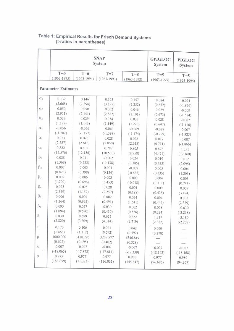
future price series in our intertemporal demand models. 4.3 Empirical Results and Their Interpretation 4.3.1 Analysis of the Estimates Comparative estimates for the SNAP, GPIGLOG and PIGLOG systems are summarised in Table 1. Empirical findings for the SNAP system are reported for four values of T (the length of consumption plan), specifically, T=5 to 8 years in Columns 2 to 5 respectively. For reasons of brevity, we only report the estimates of the GPIGLOG and PIGLOG models for T=5 years in Columns 6 and 7 respectively. Note that the results for the PIGLOG system are derived under the implicit estimation scheme rather than the standard method in order to provide a basis for comparison with the other two models. Generally speaking, the overall fit of all models as indicated by R

2 values, is quite good, given

the simplicity of our models and recalling that estimation is in share form. Nonetheless, the goodness of fits for fuel in all six cases are unreasonably low (all the R

2 values are less than

68%) provided our specification forms allow for dynamics. Possibly, the low R2

values for the fuel good equations are caused by the specification bias resulting from excluding some relevant variables from the model or using deficient functional forms. The serial properties of the error terms as shown in the DW Statistics are no longer severely pathological, although there is still evidence of positive serial correlation. Probably, this indicates the appropriateness of the correction for autoregressive errors. For the SNAP system, the most important point to highlight from these estimates is that the value of T has only a slight impact on the overall estimates. That is, changing the length of the consumption plan does not significantly change the overall results of the SNAP system. This impression is confirmed if we compare the point estimates of the coefficients, the R

2s

and the D-W statistics shown in Column 2 with those in Columns 3, 4 and 5. It is also noteworthy that the point estimates of µ are very large ranging from 1000 to 3210. This evidence is consistent with the argument that preferences are not intertemporally additive. On the other hand, the estimates of µ in all cases are insignificantly greater than zero, suggesting these estimates may suffer from the problem of multicollinearity. Another noteworthy finding is that for T=5 years, there are large differences among the values for αi and δ from the SNAP system and those from the GPIGLOG and PIGLOG systems. This is hardly surprising since the SNAP system is more general than the other two systems in allowing far more flexible modelling for the lagged and future price effects.

19

We should note, however, that the violations of the monotonicity (RΠ3

and RΠ4) and

convexity requirements (RΠ6) are caused by the negative estimates of some parameters (αi,

and βi), which is a disappointing aspect of the three intertemporal demand systems. Interestingly, the SNAP system outperforms the other two systems as far as regularity properties are concerned. Though constrained estimation would be a simple option to deal with this problem, these irregular features might be caused by other factors such as insufficiently robust functional forms, the application of an essentially micro theory specification to macro data, and the rather high level of aggregation of our series. Variations on the specifications in intertemporal Frisch demand context need to be investigated along with these other potential sources of irregularity. Consider now the nested tests of the three demand models, which may have important implications for the choice of intertemporal preference structures. All the tests have been done by using the chi-squared (χ

2) based likelihood ratio test, and the results are summarised

in Table 2. The following comments are in order. First, although Table 1 shows that η is insignificantly different from zero, the PIGLOG system is rejected in favour of the GPIGLOG system on the basis of a likelihood ratio test. It can be seen that, in all cases, the calculated χ

2

values range from 6.43 to 7.38, which exceed the critical value of 5.024 for the 2.5% significance level. Thus, the freeing up of η given µ=0 is desirable on statistical grounds. Second, for all values of T, the PIGLOG system is heavily rejected in favour of the SNAP system which, in its simple intertemporally additive form, is itself rejected in favour of its generalisation SNAP. Third, the results show that, analogously, in all cases the intertemporal additivity hypothesis maintained by the GPIGLOG system is rejected in favour of the SNAP system. Intuitively, it seems that the SNAP form is the preferred preference structure and represents a substantial improvement over the time additive structure for our data. This essentially supports Browning (1991) and Molina and Rosa's (1997) conclusions in which the intertemporal additivity hypothesis is decisively rejected. The overall similarity between our results and those of Browning, Molina and Rosa is, however, quite striking, because this study employs a different set of data, and more importantly, employs a testing methodology which is different and more general than any earlier time additivity tests. Since the SNAP system is the preferred intertemporal demand model, in the next subsection the coefficient estimates of SNAP system for all values of T are used to compute the point estimates of the intertemporal substitution elasticities. 4.3.2 Analysis of the Elasticity Estimates Table 3 presents the estimates of intertemporal substitution elasticities for T=5 to 8 years. These elasticities are defined in (30) and are computed using the coefficient estimates of the SNAP system. Notice that the column labelled T = T'(T'= 5 to 8) reports the elasticity estimates associated with the assumption that the length of consumption plan is equal to T' years. On average, the intertemporal substitution elasticity of consumption e

CtFr

in all cases is

positive and larger than one, although it is decreasing with the length of consumption plan.

20

This evidence points to a substantial positive relationship between current period consumption growth and the price of utility, which contradicts Altonji and Ham (1990), Bover (1991), Browning (1989) and Kim's (1993) results, wherein they found little prima facie evidence of a higher degree of intertemporal substitution. We also find that the commodity specific intertemporal substitution (or the price of utility) elasticities e

X ritF

are positively large but they are not very different from each other. Thus, it

appears that consumption of each commodity is equally sensitive to changes in price of utility. Interestingly, the largest degree of utility price responsiveness among the budget set is shown by other goods (for T =5 and 6 years) and by food (for T =7 and 8 years), whereas the smallest degree of utility price responsiveness is shown by fuel (for T =5 and 6 years) and by other goods (for T =7 and 8 years). Casting some light on the intertemporal lagged price e

X pitF

it−1*

and future price eX pit

Fit+1*

elasticities, results indicate that the effects of lagged and future price changes on commodity demands are fairly insubstantial. In particular, alcohol and tobacco, clothing and fuel display insignificant auto effect, generally exhibiting elasticities very close to zero. It might be concluded that these three commodities are autoindependent. While the point estimates of lagged and future price elasticities are very small, several points should be made. First, food is found to be slightly autocomplementary for all values of T. Second, the signs of these elasticities are very sensitive to the length of consumption plan. For instance, durable goods are slightly autosubstitutable for T=5 and 6 years but slightly autocomplementary for T=7 and 8 years which are in contrast to Browning (1991) and other similar studies'results, wherein durables are highly autosubstitutable. Likewise, we find that other goods are slightly autocomplementary for T=5 and 6 years but slightly autosubstitutable for T=7 and 8 years. Third, other goods exhibit the strongest auto effect relative to the remaining items in the budget set. Fourth, the signs and magnitudes of the future price elasticities e

X pitF

it+1*

are very

similar to those of the lagged price elasticities eX pit

Fit−1* , thereby indicating that the effects of

future prices on current demands are very comparable to those of lagged prices. 5 . C O N C L U S I O N The objective of this paper is twofold. First, we re-examine the testing of the conventionally maintained intertemporal additivity hypothesis. To do so, we utilise Browning's (1991) SNAP structure to build up a consumer's profit function, which nests intertemporal additivity in a simple way. Although the analysis of this paper centers around Browning's framework, it is more flexible in allowing the estimation of Frisch demands, for which it is not necessary to have closed functional forms for the Marshallian demand equations, nor for the Marshallian price of utility function. The technical aspects on how to estimate this type of Frisch demands have been discussed in considerable detail. In particular, an advanced method based on the numerical inversion approach developed by McLaren et al. (2000) is adopted to deal with the unobservability of the price of utility. The overall results reported in Section 4 suggest that this method is operationally feasible. Thus, we have opened up a wider range of utility consistent demand specifications in intertemporal analyses.

21

Our second objective is to modify Browning's approach to the specification of Frisch demand systems. The theoretical novelty in our method is in the endogenisation of the price of utility, which is based on the theoretical relationship between price of utility and total outlay without introducing the endogeneity problem. Applying this modified approach with an appropriate estimator to the Australian disaggregate data, we find that the intertemporal additivity hypothesis is decisively rejected, which lends strong support to Browning's SNAP structure. Results also reveal that expanding the length of the consumption plan does not do much violence to the data. Moreover, most of the commodities are slightly autocomplementary with themselves whereas one-period lagged and lead prices do not play a very important role in determining current demands. The failure of some observations to satisfy the required monotonicity and convexity conditions might reflect the quality of the data. More likely, this casts doubt on the reliability of the parametric forms of our demand systems or the level of aggregation of our data series. A valid suggestion on this line is to approach the specification procedure using dynamic optimisation theory as advocated by Cooper and McLaren (1980 and 1993), who exploited the duality relationship between the indirect utility function and the optimal value function in the context of an intertemporal economic model. One might want to make the demand systems more useful for policy analysis applications by specifying them in terms of more disaggregated items instead of highly aggregated items. A possible solution, in relation to this, is to impose restrictions on the structure of the profit function, which may correspond to a separability restriction. However, no such attempt is made here as these are out of the scope of this paper. REFERENCES Altonji, J. G. and Ham, J. C. (1990) Intertemporal substitution, exogeneity and surprises:

estimating life cycle models for Canada, Canadian Journal of Economics, 23, 1-43. Beach, C. M. and MacKinnon, J. G. (1979) Maximum likelihood estimation of singular

equation systems with autoregressive disturbances, International Economic Review, 20, 459-464.

Bover, O. (1991) Relaxing intertemporal separability: a rational habits model of labor supply estimated from panel data, Journal of Labor Economics, 9, 85-100.

Browning, M. J. (1982) Profit function representations for consumer preferences. Department of Economics Working Paper No. 82/125, University of Bristol.

Browning, M. J. (1989) The intertemporal allocation of expenditure on non-durables, services and durables, Canadian Journal of Economics, 22, 22-36.

Browning, M. J. (1991) A simple non-additive preference structure for models of household behaviour over time, Journal of Political Economy, 99, 607-637.

Browning, M. J. (1997) Interpreting the results of empirical analyses of intertemporal allocation: an identification problem, Economics Letters, 56, 41-44.

Cooper, R. J. (1994) On the exploitation of additional duality relationships in consumer demand analysis, Economics Letters, 44, 73-77.

Cooper, R. J. (1996) Optimal consumption-wealth relationships derived by consumer intertemporal profit maximisation, Economics Letters, 50, 341-347.

Cooper, R. J. and McLaren, K. R. (1980) Atemporal, temporal and intertemporal duality in consumer theory, International Economic Review, 21, 599-609.

22

Cooper, R. J. and McLaren, K. R. (1992) An empirically oriented demand system with improved regularity properties, Canadian Journal of Economics, 25, 652-668.

Cooper, R. J. and McLaren, K. R. (1993) Approaches to the solution of intertemporal consumer demand models, Australian Economic Papers, 32, 20-39.

De La Croix, D. and Urbain, J. (1998) Intertemporal substitution in import demand and habit formation, Journal of Applied Econometrics, 13, 589-612.

Deaton, A. (1986) Demand analysis, in Handbook of Econometrics Vol III (Ed.) Z. Griliches and M. D. Intriligator, North-Holland, Amsterdam, 1767-1839.

Deaton, A. and Muellbauer, J. (1980) An almost ideal demand system, American Economic Review, 70, 312-326.

Dunn, K. B. and Singleton, K. J. (1986) Modeling the term structure and interest rates under non-separable utility and durability of goods, Journal of Financial Economics, 17, 27-55.

Gorman, M. (1967) Tastes, habits and choices, International Economic Review, 8, 218-222. Gorman, M. (1976) Tricks with utility functions, in Essays in Economic Analysis (Ed.) M.

Artis and R. Nobay, Cambridge University Press, Cambridge, pp. 211-243. Kim, H. Y. (1993) Frisch demand functions and intertemporal substitution in consumption,

Journal of Money, Credit, and Banking, 25, 445-454. Molina, J. A. and Rosa, F. (1997) Testing for the intertemporal separability hypothesis on

Italian food demand, in Agricultural Marketing and Consumer Behavior in a Changing World (Ed.) B. Wierenga, Kluwer Academic, Boston, pp. 245-259.

McLaren, K. R., Rossiter, P. and Powell, A. A. (2000) Using the cost function to generate flexible Marshallian demand systems an initial exploration, Empirical Economics, 25, 209-227.

Ni, S. (1995) An empirical analysis on the substitutability between consumption and government purchases, Journal of Monetary Economics, 36, 593-605.

Pashardes, P. (1986) Myopic and forward looking behaviour in a dynamic demand system, International Economic Review, 27, 387-397.

Pollak, R. (1970) Habit formation and dynamic demand functions, Journal of Political Economy, 78, 745-763.

Pollak, R. and Wales, T. J. (1969) Estimation of the linear expenditure system, Econometrica, 37, 611-628.

Rimmer, M. and Powell, A. A. (1996) An implicitly additive demand system, Applied Economics, 28, 1613-1622.

Selvanathan, S. (1991) The reliability of ML estimators of systems of demand equations: evidence from OECD countries, Review of Economics and Statistics, 73, 346-353.

Spinnewyn, F. (1981) Rational habit formation, European Economic Review, 15, 91-109. Stone, R. (1954) Linear expenditure systems and demand analysis: an application to the

pattern of British demand, Economic Journal, 64, 511-527.

23

24

25

26