towards development of an iso container to spreader bar ... · 1 towards development of an iso...

Towards Development of anISO Container to Spreader Bar

Sensor System

Richard NorcrossU.S DEPARTMENT OF COMMERCE

Technology AdministrationNational Institute of Standards and Technology

Intelligent Systems DivisionGaithersburg, MD 20899-8230

NISTIR 7418

NISTIR 7418

Towards Development of anISO Container to Spreader Bar

Sensor System

Richard NorcrossU.S DEPARTMENT OF COMMERCE

Technology AdministrationNational Institute of Standards and Technology

Intelligent Systems DivisionGaithersburg, MD 20899-8230

May 2007

U.S. DEPARTMENT OF COMMERCECarlos M. Gutierrez, Secretary

NATIONAL INSTITUTE OF STANDARDS AND TECHNOLOGYWilliam Jeffrey, Director

1

Towards Development of an ISO Container to Spreader Bar Sensor System Richard J Norcross NIST Manufacturing Engineering Laboratory 100 Bureau Dr Gaithersburg, MD 20899-8230 To Oceaneering International Inc. 7001 Dorsey Rd

Hanover, MD 21076

Towards Development of an ISO Container to Spreader Bar Sensor System

2

Abstract This report describes a sensor system that determines the relative pose between a crane spreader and a standard twenty-foot shipping container (a.k.a. an ISO container). The sensor system supports efforts to transfer cargo between ships in high sea states under Office of Naval research’s (ONR’s) High Capacity Alongside Sea Base Sustainment Large Vessel Interface Lift On/Lift Off (HiCASS LVI LO/LO, HiCASS) program. The sensor system is a collection of three dimensional image sensors observing the corners of stacked ISO containers. The need to position the spreader’s twistlocks into the ISO standard corner holes set the uncertainty requirements for the sensors at σ≤ 0.9 cm. The requirement to drive the servo control loop requires the sensor system to determine the pose at 10 Hz with σ≤ 0.5 cm. The report describes alternative sensor system configurations, methods to achieve the required transfer throughput and container or spreader positioning accuracy, and potential methods for sensors to perform in bright sunlight1.

1 Certain trade names and company products are identified in an illustration, the text, or references in order to adequately specify the software, experimental procedure, or equipment used. In no case does such an identification imply recommendation or endorsement by the National Institute of Standards and Technology, nor does it imply that the products are necessarily the best available for the purpose.


3

Table of Contents Executive Summary ........................................................................................................ 5

1 Introduction............................................................................................................... 7 2 Methods, Assumptions, and Procedures..................................................................... 7 2.1 Sensor Mounting Assumptions ............................................................................... 8 2.1.1 Overhang Sensor Mount Option .......................................................................... 8 2.1.2 Side Arm Sensor Mount Option........................................................................... 9 2.1.3 Adjacent Container View Sensor Mount Option .................................................. 9 2.2 Requirements ....................................................................................................... 10 2.2.1 Range ................................................................................................................ 10 2.2.2 Accuracy ........................................................................................................... 11 2.3 Frequency............................................................................................................. 12 2.4 Detection Algorithm............................................................................................. 13 2.4.1 Target................................................................................................................ 13 2.4.2 Model Match ..................................................................................................... 14 2.4.3 Sparse Model Match.......................................................................................... 15 2.4.4 Edge Pattern Match ........................................................................................... 15 2.4.5 Intensity Image Detection.................................................................................. 16 2.5 Sensor Fusion....................................................................................................... 16 2.5.1 Four Corner Solution......................................................................................... 16 2.5.2 Three Corner Solution ....................................................................................... 17 2.6 Daylight Operation............................................................................................... 17 2.7 Sensor Selection ................................................................................................... 17 2.8 Sensor Position Calibration .................................................................................. 18

3 Results and Discussions........................................................................................... 18 3.1 Precision Requirement.......................................................................................... 18 3.2 Feature Detection ................................................................................................. 19 3.3 Frequency Results ................................................................................................ 20 3.4 Daylight Tests ...................................................................................................... 21 4 Conclusions............................................................................................................. 23

5 Recommendations ................................................................................................... 23 5.1 Sensor Selection ................................................................................................... 23 5.2 Computer Power................................................................................................... 24 5.3 Sensor Mounting .................................................................................................. 24 5.4 Pose Reference ..................................................................................................... 24 6 References............................................................................................................... 25


4

Table of Figures Figure 1 a) ISO corner and b) Dual Cone TwistLoc......................................................... 8 Figure 2 Mounting Options, (a) Overhang, (b) Side Arm, (c) Adjacent View .................. 8 Figure 3 Stereo Camera Disparity vs. Range ................................................................. 11 Figure 4 Passive Target ................................................................................................. 14 Figure 5 Precision Requirement Estimation................................................................... 19 Figure 6 Gray Board Image from Initial Flash LADAR in Sunlight............................... 21 Figure 7 Grey Board Image from PMDTec Flash LADAR............................................ 22 Figure 8 Stereo Camera in Sunlight, (a) without filter (b) with filter.............................. 22 Figure 9 LADAR Scan Across ISO Corner on box........................................................ 23


5

Executive Summary The Office of Naval Research (ONR) conducts research and develops capabilities to support future Sea Base operations of the U.S. Navy. The High Capacity Alongside Sea Base Sustainment Large Vessel Interface Lift On/Lift Off (HiCASS LVI LO/LO, HiCASS) program is developing a crane system to transfer up to twelve twenty-foot shipping containers (ISO containers) per hour between two large vessels while underway in the upper limits of Sea State 4. Among the challenges facing HiCASS development is the accurate and timely measurement of the relative position between the crane’s spreader and the container on the delivery ship.

The lone common attribute of sea borne containers is the shape and position of the corners. We, therefore, developed the capability to track the container by observing the corners with discreet sensors. Since the spreader obscures the corners of the target container during acquisition, the sensors observe the corners of the adjacent containers and the system infers the target container’s pose from them. The adjacent corners may be observed directly or by distinctive targets placed on them.

This report summarizes the use of flash LADARs (Laser Detection and Ranging) and stereo vision cameras to determine the location of the ISO container. Both flash LADARs and stereo cameras are planar sensors that generate a range value for each pixel. The lateral position of the pixel and the range at that pixel define a point in three dimension space. Flash LADARs measure range through the reflection of a continuous amplitude-modulated light beam. The stereo cameras sense reflected ambient light and detect depth through binocular disparity. Each sensor observes and locates an ISO corner adjacent to the target container. The sensor system fuses the individual locations to produce the pose of the container. The sensor system reports the container pose with sufficient accuracy and frequency for the crane’s controller. We base the accuracy requirement on the tolerance between the twistloc cones on the spreader and the hole in the horizontal surface of the container’s corners. To fulfill the peg-in-hole requirement, the individual sensors measure the location of the adjacent corners with uncertainty ≤ 1.8 cm (U ≤ 1.8 cm). The controller also uses the sensor data in a high gain servo control loop. For use in the servo loop, the sensors must determine the position with U ≤ 1.0 cm. The crane controller sets the control cycle frequency requirement at 10 Hz based on ship motion simulation. Since the time to acquire the raw sensor data is set, we modify the detection algorithms to meet the time requirement. These modifications force the accuracy to the limits given above.

HiCASS must transfer cargo at all times of the day. Therefore, the sensor systems must operate in darkness and in bright sunlight. 3D sensors readily operate under artificial lights but are overwhelmed by the high ambient light (80+ klx) common on clear days. This report investigates the current ambient light limits. Neutral density filters enable the


6

stereo vision cameras to operate at over 100 klx. Similarly, a scanning LADAR2 operates in all ambient light conditions. The sensor system measured the pose with sufficient accuracy and frequency to guide the controller of the HiCASS testbed. However, the performance was marginal. The controller’s requirements exceeded the initial goals of the research. Therefore, recommendations are as follows:

1. The HiCASS sensor system should utilize high resolution sensors (e.g. 1024 pixels x 768 pixels) for improved lateral resolution.

2. The stereo vision depth detection should be augmented with a scanning LADAR.

3. The sensor system should utilize a hierarchy of computation platforms to support richer data evaluation algorithms.

4. The sensors should be mounted to limit the sensor range requirements. 5. The target container’s pose reference should be as close to the detected feature as

possible to reduce errors due to extrapolation.

2 A scanning LADAR is a 2D sensor that detects a pulsed laser to determine ranges along a line.


7

1 Introduction The High Capacity Alongside Sea Base Sustainment Large Vessel Interface Lift On/Lift Off (HiCASS LVI LO/LO, HiCASS) is a five year, ONR funded, program to develop cargo handling capability for future Sea Base operations. In 2005, the ONR awarded the HiCASS contract to Oceaneering International, Inc (OII). OII is to investigate and build a crane system that can transfer up to twelve twenty-foot ISO containers per hour between two large vessels while underway in Sea State 4 and above. OII intends to develop the technology and demonstrate progressive improvements in capabilities towards a full-scale prototype in Fiscal Year 2010.

HiCASS development faces fundamental challenges in skin-to-skin operations and payload transfer. The payload transfer requires reach, speed, and motion compensation that are unprecedented in sea borne cranes. Adequate motion compensation requires an advanced control system that includes positive payload control, innovative power and energy storage, motion sensing, and motion prediction. The motion sensing measures the relative position between the two ships and the relative position of the crane spreader and the ISO container. OII requested that NIST evaluate sensors to be used to track these relative motions. This report covers the spreader-to-container relative motion and concludes with recommendations for the enhancement of the sensor system.

2 Methods, Assumptions, and Procedures The spreader-to-container sensors track the position and orientation of an ISO container during the acquisition of that container or during the delivery of another container. ISO containers come in numerous types and subclasses, including general purpose (code G), thermal (code H), open top (code U), and tank (code T) containers. The lone common attribute of sea borne containers is the shape and position of the corners. Therefore, our methods and procedures track the ISO containers by observing their corners. Section 8.4.3 of the “Ship-to-Ship and Container-to-Spreader Sensors Specification” [1] defines the container position as the center of the four upper ISO corners with the X-axis aligned with the long axis of the container, the y-axis aligned with the short axis of the container and the z-axis perpendicular with the plane defined by the tops of the four upper corners. We therefore, develop means to combine observations of several corners and project their position to the position reference point. These corners are the only features common to all ISO containers. Figure 1a shows a typical ISO corner. The spreader has cones that insert into the corners, then twist to secure the spreader to the container. When stacking containers, the container carries similar cones (Figure 1b) to attach the container to the container below. The container-to-spreader sensors measure the position of the spreader from the container.


8

Figure 1 a) ISO corner and b) Dual Cone TwistLoc

Reference [3] defines the container size from the outer corner surfaces but does not specify the size, shape, or position of the container’s sides, roofs or floors. Therefore the sensors track the locations of the ISO corners. The sensors must identify unique features to track. The sensors may track the corner’s upper surface, edges, or an artificial target mounted on the corner.

2.1 Sensor Mounting Assumptions NIST considered three alternatives for mounting the spreader-to-container sensors (see Figure 2). The first alternative tracked the subject container directly from the spreader. The next placed the sensors on arms that reached around the container to view the corners of the subject container. The third alternative tracked the ISO corners of adjacent containers and inferred the position of the subject container. Most of the efforts in this report used the third option.

OCEANEERING

OCEANEERING

OCEANEERING

OCEANEERING

OCEANEERING

OCEANEERING

(a) (b) (c) Figure 2 Mounting Options, (a) Overhang, (b) Side Arm, (c) Adjacent View

2.1.1 Overhang Sensor Mount Option The HiCASS sensors guide the spreader cones into the target container’s corners. For the container delivery situation, the sensors must observe the target container around the outside of the carried container. To determine the observation angle we consider a typical twist lock configuration. The twistloc attaches to and protrudes approximately 10.8 cm (4.2 in) from the container’s lower corner. The ISO corner hole center is 10.2 cm (4 in)


9

from the outside edge of the ISO corner (Figure 1). Therefore, the minimum angle to observe the hole during mating is 46.4°. ISO recognizes 13 freight container designations [3]. The designations vary the container’s length and height. HiCASS concentrates on the 1CC Freight Container Designation, which is 6.058 m (19 ft 10.5 in) long and 2.591 m (8 ft 6 in) high. Therefore the spreader mounted sensor is 2.6 m (102 in) above the container bottom and, to observe the ISO corner hole as the cone enters, must be more than 2.5 m (97 in) to the front of the spreader. Since a sensor overhanging the container by 2.5 m would interfere with the next stack of ISO containers, this configuration is clearly impractical.

As an alternative, we reduce the overhang distance by increasing the drop zone. The drop zone is the distance above the ISO corner that the controller commands motion without feedback, i.e., via open loop control. Section 8.5 of [1] determines the maximum angle to view the lower ISO container without impacting the adjacent container as 28°. At this angle, the twistloc cone will be 8.4 cm (3.3 in) above the ISO corner as the sensor looses sight of the ISO corner hole. OII decided an 8.4 cm drop height is excessive and NIST considered alternative mounting positions.

2.1.2 Side Arm Sensor Mount Option A sensor mounted near the bottom of a carried container maintains a clear view with zero drop distance and minor overhang. This option mounts the sensors on arms that hang alongside the container. The arms require a significant mechanical support system to adjust for when a container is carried or being acquired and to retract for access to interior cells.

The 1Cx Freight Container Designations allow two nominally 6 m (20 ft) containers to mount in the shipboard space for one 12 m (40 ft, designation 1Ax) container. Thus the side arm is deployable on only one end of the container. The observations of two ISO corners from a single end provide sufficient data to determine a 5 degree-of-freedom (5 DOF) position of the container. This option requires the container’s pitch to be measured by the ship-to-ship sensor. Pitch is a few degrees with a long period (e.g. 6 s). Furthermore, the pitch can be several degrees off as the mated corners at one end force the proper alignment as the other end comes together[1].

The side arm option has several advantages. The sensor interpretation is identical for both acquiring and delivering a container. The sensor is always close and may be mounted at an optimal distance for the sensor. The arms can also carry actuators for the twistlocs, reducing the crew requirements. OII rejected the side-arm option primarily on the limited pose detection.

2.1.3 Adjacent Container View Sensor Mount Option This sensor configuration observes the ISO corners of containers adjacent to the target container. Based on the relative positions of the containers, the sensor algorithm infers the target container’s pose from the positions of the adjacent corners. Four or six sensors


10

observe adjacent corners from a near vertical position. This configuration is the basis of the subsequent sensor development. The HiCASS crane design suspends the spreader bar from the gantry trolley with a RoboCrane based micro-manipulator. RoboCrane generates 6 degrees of controlled motion through a system of computer controlled cables between a larger upper platform (at the trolley) and a smaller lower platform (at the spreader bar). The cables, therefore, pass immediately over the adjacent containers. The areas above and to the sides of the container must, therefore, be clear for the cables to operate. This requirement limits the permissible container stacking configurations.

Section 7.7.5 of [1] lists the possible container configurations. Each possible container stacking case (cases 1, 2, 6, 7, 9, 10, and 11) has the adjacent container within one level of the spreader bar. Therefore, sensors mounted at the spreader bar observe an ISO corner at one of two distances. The corner is either immediately below the spreader (called the “near problem”) or one container height away (called the “far problem”). The Freight Container Description ISO standard specifies the gap between two 6 m containers occupying a 12 m container position is 76 mm (3 in). The adjacent side container’s position is not set by standards but is always parallel to the target container. Therefore the pair of ISO corners on the end defines the athwart ships vector while the pair of ISO corners on the side adjacent container specifies the orthogonal fore/aft vector. These vectors, along with the midpoints of the ISO corner pairs, define the 6 DOF pose of the target container.

This configuration requires eight sensors. Each sensor mounts above one of the adjacent ISO corners; two mount to port, two to starboard, two forward, and two aft. Two or three sets of sensors can view adjacent corners during a particular lift. Based on the possible container stacking, either the forward or aft set and either the port, starboard, or both athwart ships sets are over an adjacent container.

2.2 Requirements The spreader to container sensor must have sufficient range and accuracy, at a specified frequency. The range requirement is based on the division of labor between the ship-to-ship sensor and the spreader-to-container sensor. The accuracy requirement is based on the ultimate need to insert the four cones of the spreader into the four corners of the ISO container. The frequency is set by the controller developers based on expected motion.

2.2.1 Range The HiCASS control system uses two sensor systems to track and acquire the ISO container target. The ship-to-ship sensor detects the relative positions of the cargo ship to the crane ship to within 0.3m (1ft). The control system brings the spreader bar to within the proximity of the container based solely on the ship-to-ship sensor. The spreader-to-container sensor must track the ISO container during the final meter of the approach.


11

The actual distance of the “final” meter depends on the configuration of the container stacks. When the spreader acquires a container from a flat configuration, the final meter is from 0 m to 1m (39”). When the spreader deposits a container to a flat configuration, the final meter of approach ends at the height of the container 2.6 m (8.5 ft). We refer to the previous situation as the “near problem” and the later situation as the “far problem”. Based on the configuration of the containers, an approach may be part near and part far. Since the spreader must carry a container, the spreader-to-container sensors must overhang the spreader and be retractable for entering confined spaces. Therefore the sensors mount to the upper edges of the spreader, which are roughly 1m (3ft) above the cones that actual engage the ISO corners. The near problem, therefore, requires the sensors to track the ISO corners from 1 m to 2 m. The far problem requires the sensors to track from 3.6 m to 4.6 m (11.8 ft to 15 ft). We concentrated on the near problem. Stereo vision cameras have an inverse relationship between the distance to an object and the resolution of that distance. Thus as the object moves away, the sensor system’s ability to precisely measure the range decreases. Since the lateral position is a function of the range, the precision of all motion measurement diminishes. Figure 3 (Stereo Camera Disparity vs. Range) shows the computed depth from the disparity from the sensor’s interface software. A unit disparity represents 36 cm (14 in) of motion at the “long problem” (4.2 m) range.

Figure 3 Stereo Camera Disparity vs. Range

The flash LADAR sensors also have an inherent difficulty with the “far problem”. The flash LADAR’s resolution is improving but remains much less than common cameras. The initial flash LADAR sensor uses a 64 pixel x 64 pixel detection array[6]. For the far problem, each pixel covers more than 25 cm2 (3.9 in2 ), which far exceeds our accuracy requirement. We, therefore, concentrate our efforts on the near problem and review possible solutions for the far problem.

2.2.2 Accuracy The accuracy requirement depends on the use of the sensor data. We base our efforts on achieving the position accuracy to insert the cone into the ISO corner hole (peg-in-hole).


12

The sensors must generate a pose with sufficient accuracy to allow the controller to guide the cone into the holes in the four corners of the ISO container. Since the cones cover the holes of the ISO corners during insertion (section 2.1), the sensors must infer the pose from observable features on adjacent containers. Therefore, the sensor accuracy depends on the tolerance between the cone and the hole in the ISO container corner and on the effect of inferring the pose from the adjacent corners. Reference [4] sets the dimensions of the corner of the ISO container to be 15.2 cm x 17.7 cm (6 in x 7 in) with a countersunk 7.6 cm x 10.2 cm (3 in x 4 in) oblong hole in the top. Although normal use dents the cone tip, we assume the cone maintains a near point for our calculations. Therefore, for proper insertion, the relative position of the cone tip to the ISO corner hole must be within ±3.8 cm (±1.5 in) in the athwart ship direction and ±5.1 cm (±2 in) in the fore-aft direction. We allocate the error between the sensors and the manipulator’s mechanical system. Only that portion of the mechanical system between the sensors and the cone tip are significant to the problem. We therefore assign 2.5 cm (1 in) of the available tolerance to the sensors and remainder to the manipulator. The sensors measure the adjacent corners, not the actual corners. We determined the required accuracy through a simulation of the effects of detection errors on the final pose calculation. The simulation took the positions of four adjacent corners, calculated the target pose, projected the target pose into the far corner from the observed corners, and determined the final error to the actual corner position. The simulation introduced normally distributed errors into the position of the observed corners and returned the standard deviation of the reference corner. Experimenters adjusted the magnitude of the standard deviation of the induced errors and observed the effect of the final error. We use the magnitude of the Prediction Interval to evaluate the accuracy of the sensor [5]. The prediction interval uses the distribution of sample readings to predict the distribution of the next reading within a desired certainty.

!ntn"1,# 2

1+ 1 m where n is the number of simulation samples (1000), α is 0.1, and m is the samples to be averaged in the final reading (1). Thus the prediction interval is 2.32 times the standard deviation of the simulation samples. The results of the simulation are in Section 4.

2.3 Frequency The HiCASS control system expects new data at 10 Hz. Thus the sensor system must acquire the data, interpret the general features (depth, edges, etc), determine the specific features (holes, corners, etc.), compute the target position, compute the target container’s pose, and transmit the value within 100 ms. The sensor manufacturer’s software acquires the data and interprets the general features. The computation of the container pose from the observed features and the value transmission is set by the interface requirements (both sensor mounting and


13

communications). Therefore we must adjust the feature detection and location calculation to meet the frequency requirement.

2.4 Detection Algorithm Each sensor detects a feature on a container adjacent to the target container. The sensor system uses an algorithm based on the details of the feature and the capabilities of the particular sensor.

2.4.1 Target A target is a device that assists the detection of a feature. We design the target to have a high signal-to-noise ratio making the target both easy to identify and providing a repeatable reading. The target also places additional responsibilities on the ship’s crew that may be undesirable.

The face of the target has cross made of a highly reflective material (approximately 2000 times brighter than a diffuse white surface [2]) on a flat black background (Figure 4). The high reflectivity saturates the sensor’s individual pixels and simplifies their identification. The pixels adjacent to the cross provide the range data necessary to compute the Cartesian position of the target. The target detection algorithm makes four passes across the data. The first pass collects the saturated pixels. The second pass removes pixels saturated by spurious noise. The third and fourth passes identify the center row along each column and the center column along each row of the saturated pixels in the image. A linear regression of the center rows defines the vertical arms of the cross and a linear regression of the center columns defines the horizontal arms of the cross. The intersection of these two lines is the center of the cross.

The Cartesian location of the target is a function of the cross’s center and the distance to the target. Since the cross’s pixels are overwhelmed, the sensor cannot determine the range to them. However, the pixels along the outer edge of the cross continue to provide range data. The detection algorithm converts the cross’s center to Cartesian coordinates with the range data from along the cross’s edges.


14

Figure 4 Passive Target

The target is approximately 15 cm x 17 cm (6 in x 7 in) and centers on the ISO corner hole via a like-shaped extrusion on the target’s underside. With the extrusion, the target mounts on an adjacent ISO corner. An alternative mounting is required for direct observations of the target container.

A target improves the system performance in both accuracy and speed. However the target also adds a burden to the deck crew of the container ship. When an artificial target is inappropriate, the sensor system must observe, identify, and track the ISO corner directly. HiCASS hopes to avoid using targets if possible.

2.4.2 Model Match When artificial targets are not available, the sensors must identify the ISO corner directly. The ISO corner is a 16.3 cm x 17.7 cm (6.4 in x 7 in) steel or aluminum block with holes on the outboard sides. The international standard[3] specifies the corner’s size, the position of the holes, and the radii of the various edges. However, a review of three sets of ISO corners discovered the block size and edge radii varied. Only the hole and its relative position to the outboard sides were reliably consistent.

Stereo cameras and flash LADARs are 3D image devices. Each pixel in the image includes a depth value which, when combined with the pixel location yields a 3D position. This algorithm uses the 3D positions to identify the ISO corner. The algorithm uses three features of the ISO corner: the top surface, the hole, and the outside edges. A histogram of the pixels around the center of the image produces a data line with many local maximums. A filter removes the zero values and the high frequency peaks leaving a multi-modal response. The smallest mode is the closest range and the nominal depth to the ISO corner. Based on the nominal depth, the algorithm generates a model of the ISO corner where each pixel has an expected depth interval. The algorithm then checks the model against the pixels in the image and determines which position most closely matches the model.


15

The algorithm is slow when the image is large or when the target is close and the model becomes large. As time constraints became restrictive, researchers developed a sparse model that was unaffected by the target range.

2.4.3 Sparse Model Match The sparse model match is similar to the model match described above. The algorithm uses the same ISO corner features. However the algorithm searches on a grid of pixels rather than each pixel. The accuracy requirement of the measurement determines the size of the grid.

From the nominal depth the algorithm determines the number of pixels per a predetermined distance. The algorithm then determines the pixel spacing for a grid of that size and tests the points on a grid for the appropriate range to the sensor. For example, athwart ships from the ISO corner should be a gap, i.e., a depth several centimeters greater then at the ISO corner’s surface. The algorithm checks points on a 1.3 cm (0.5 in) grid, which covers a 50 mm x 230 mm (2 in x 9 in) area. If sufficient pixels report an appropriate depth (e.g., 80 of the 95 pixels have a range 8 cm (3 in) or greater than the reference pixel’s depth), the algorithm continues with the fore/aft gap, the surfaces around the hole, and area of the hole. The algorithm checks 278 points, then averages the pixels with the greatest matches to generate the final value. The final averaging compensates for noise and improves final accuracy. The algorithm is simple, robust, and takes the same computation effort whether the target is far away with a small image or close with a larger image. The disadvantage of the pattern match algorithm is the accuracy is only slightly better than the size of the grid spacing. Finer grid spacing increases accuracy but consumes more time. Even a minimal grid across the entire image takes more time then is available for the OII demonstrator. Thus the algorithm limits the search to the area around the previous point.

2.4.4 Edge Pattern Match The stereo sensors identify edges in the image as a precursor to determining the range. The edge pattern match algorithm uses this edge data to locate the ISO corner. The edge detection algorithm compares only the positions of expected edges since data noise made evaluations based on an expected smooth area unreliable. The edges are a known distance from the reference point and the algorithm checks at the equivalent pixel. If the pixel size is incorrect, the algorithm misses the edge. To accommodate minor distance and angular errors, the algorithm counts a half match for edges found at the adjacent pixels. The edge pattern algorithm is highly dependent on an accurate pixel size. When the pixel size is incorrect, the algorithm searches the wrong line and cannot identify the edge. The edge pattern match works better at longer ranges since the resolution of the pixels is less and more forgiving. Also at greater distances there are fewer spurious edge readings between the actual edges.


16

2.4.5 Intensity Image Detection 3D optical sensors (both stereo vision and flash LADAR) generate an intensity image along with the depth image. The intensity image is significantly less noisy than the associated depth image. Therefore, where low noise readings are desired, the intensity image can provide a more stable reading. The disadvantage of the intensity image is the algorithm relies on shadows. When ambient light distorts the shadows, the sensor system must rely on an alternative method. Therefore the sensor system uses this algorithm only in the immediate vicinity of the last reading.

The hole in the ISO corner is a fairly reliable shadow. The algorithm checks nine points around the location of the last location and takes the darkest reading as a position in the hole. The algorithm locates the edges of the hole along the row and along the column of the darkest point. The mid-point of the row edges is the column center and the mid-point of the columns is the row center. The algorithm detects the edge of the hole by a transition in the intensity image. The algorithm derives the transition threshold from a histogram of the local data. The histogram produces a bi-modal data line. The lower (i.e., darker) mode is the hole and the upper (i.e., lighter) mode is the ISO corner surface. The edge intensity is the lower side of the upper mode. The algorithm checks the value for each row (or column) pixel and reports the first pixel to cross the threshold as the edge. The software makes two passes through the basic algorithm to correct corner effects. Next, the algorithm combines five rows and five columns to overcome the noise along the edges. Under appropriate lighting, this algorithm gives accurate, stable, and quick readings.

2.5 Sensor Fusion The controller interface specifies that the sensor system report the container position as the location of the center of the positions of the upper surface of the four top ISO corners. This location is not a physical component. The detection algorithms must infer the position from observations of other objects. As stated in Section 2.1.3, the sensor observes the location of the corners of adjacent containers.

2.5.1 Four Corner Solution The permissible container stacking configurations ensure four adjacent corners are available. One pair of corners is along the end of the target container. The second pair is along either the port or starboard side of the target container. There may be a third pair along the opposite side of the target container. The Four Corner Sensor Fusion algorithm combines these four positions to determine the pose of the target container. The algorithm computes the mid-point and vector between each pair of observed corners. The vector from the end pair defines the athwart ships vector (y), while the athwart ships pair defines the fore/aft vector (x). The vertical vector (z) is the cross product of these two vectors. The reference position is the intersection of the midpoint positions projected


17

along the opposing vector and adjusted for a vertical difference. The vertical difference may be based on differences in the readings or based on known container heights. NIST used the Four Corner Solution to determine the accuracy requirements for the peg-in-hole solution.

2.5.2 Three Corner Solution The available computer equipment was not fast enough to process data from four sensors within the frequency requirement for HiCASS. Therefore, NIST developed a three sensor fusion algorithm for use on the OII test bed.

The three corner solution relies an a priori knowledge of the relative position of the observed corners to the reference point. The three corner solution uses the two corners adjacent to the end of the target container and one corner to the side of the opposite end. The two corners at the one end align with the athwart ship axis (y). The third corner and one of the first two define a vector nearly along the fore/aft vector. The cross product of these vectors defines the vertical vector (z). The cross product of the vertical vector and the athwart ships vector defines the true fore/aft vector (x). The average position of the three observed corners defines a point, which is a known distance and orientation from the reference point. Thus the sensors report a position which is the average of three corner points offset predefined distances along the athwart ship and fore/aft vectors. The three corner solution uses a combination of interpretation (the averaging) and extrapolation (the offsets) to determine the pose of the target container. The averaging diminishes the sensor noise, while the extrapolation amplifies the noise.

2.6 Daylight Operation HiCASS will operate at sea during both day and night. During night operations, HiCASS will control the target illumination. However, HiCASS must contend with ambient light during daylight operations. Ambient daylight ranges from 1000 lx for an overcast day, 10-20 klx for indirect sunlight (i.e., shadows), and 100-130 klx for direct sunlight on a clear day. Most 3D sensors, including the ones used in this effort, are not designed for daylight operations. We therefore identify the operating limits of the sensors and identify methods to extend those limits. The initial daylight tests used a 10 panel gray board. The 10 panels were various shades of gray, from white to black, and allowed researchers to observe the response range of the sensor. The initial tests were disappointing and the test discontinued. Subsequent tests observed the sensors observing ISO corners in a pass/fail mode.

2.7 Sensor Selection NIST investigated two types of sensors: flash LADAR and stereo vision. We began and performed most of the preliminary work with a stereo vision camera [8] and a low


18

resolution flash LADAR [9]. We converted to a higher resolution flash LADAR [7] due to some integration constraints. Each sensor generated a three dimensional position of a single ISO corner. Software combined the 3D positions into a 6 DOF pose as per Section 2.5. Near the conclusion of the effort, NIST reviewed a scanning LADAR sensor [11] with the concept of fusing the scanning LADAR output with the stereo vision output to generate a single 3D position. With each sensor, NIST used the manufacturer’s acquisition and interpretation software as provided through a set of dynamic link libraries (.dll). This software was convenient but was not necessarily the fastest, most efficient, nor most accurate available. Software shortcomings did limit the investigation of some sensors.

2.8 Sensor Position Calibration The sensor system infers the pose of the target container through observations of features on adjacent containers. Proper pose calculation requires knowledge of the sensors’ positions relative to the spreader reference point. Since the control system guides the spreader bar onto the target container on a nearly vertical path and along this path the individual sensors remain nearly vertical to the subject feature, we calibrate the sensor position along the approach path. This calibration is simple and can be easily performed in the field.

The calibration procedure begins with the spreader attached to the target container. We record the sensor readings and the transformations required to generate the proper target pose. The controller then holds the spreader (either by cable position or by mechanical spacers between the spreader and target) at points along the approach path. We record the sensor readings and the required transformations at these points. These readings and transformations are the system calibration.

At run time, the sensor system detects the feature position for each sensor. The system adjusts the feature position according to the calibration data. Between taught points, the system uses a linear interpolation of the nearest points. The system then uses the adjusted feature positions to compute the target pose in accordance with Section 2.5.

3 Results and Discussions

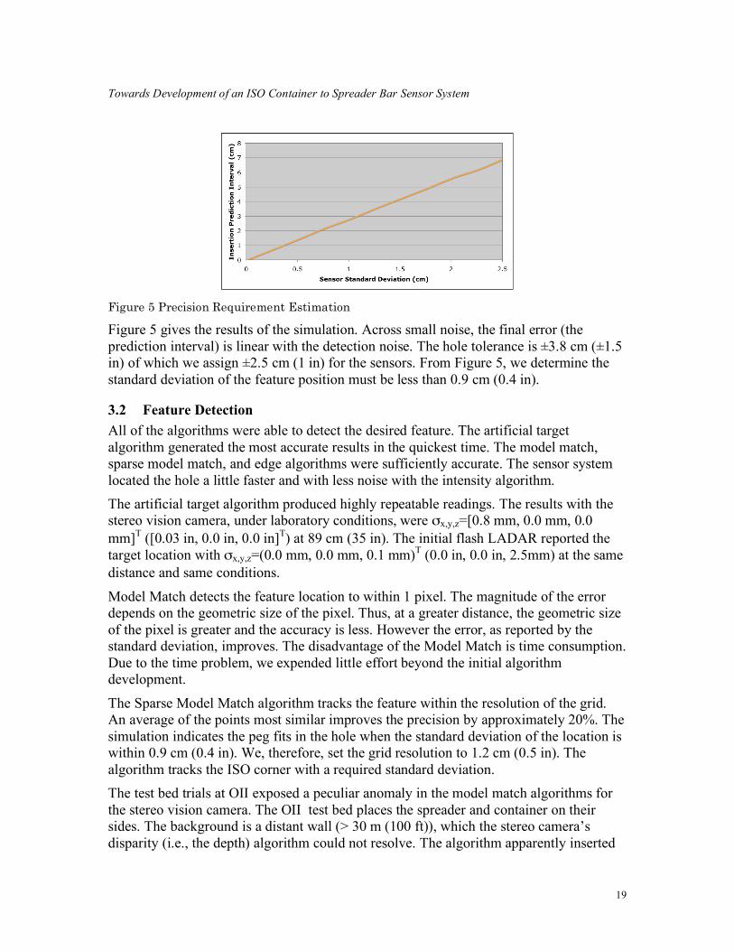
3.1 Precision Requirement We determine the precision requirement for the sensor from the precision required to place the cone into the ISO container’s corner. The sensor algorithm infers the pose of the container from the detection of the location of several features. Thus we create a computer model of the pose calculation and introduce noise into the feature positions. The algorithm computes the container’s position and orientation. Then, based on the orientation, the algorithm computes the position of the container’s far corner. The magnitude of the prediction interval of that position is the system error.


19

Figure 5 Precision Requirement Estimation

Figure 5 gives the results of the simulation. Across small noise, the final error (the prediction interval) is linear with the detection noise. The hole tolerance is ±3.8 cm (±1.5 in) of which we assign ±2.5 cm (1 in) for the sensors. From Figure 5, we determine the standard deviation of the feature position must be less than 0.9 cm (0.4 in).

3.2 Feature Detection All of the algorithms were able to detect the desired feature. The artificial target algorithm generated the most accurate results in the quickest time. The model match, sparse model match, and edge algorithms were sufficiently accurate. The sensor system located the hole a little faster and with less noise with the intensity algorithm. The artificial target algorithm produced highly repeatable readings. The results with the stereo vision camera, under laboratory conditions, were σx,y,z=[0.8 mm, 0.0 mm, 0.0 mm]T ([0.03 in, 0.0 in, 0.0 in]T) at 89 cm (35 in). The initial flash LADAR reported the target location with σx,y,z=(0.0 mm, 0.0 mm, 0.1 mm)T (0.0 in, 0.0 in, 2.5mm) at the same distance and same conditions.

Model Match detects the feature location to within 1 pixel. The magnitude of the error depends on the geometric size of the pixel. Thus, at a greater distance, the geometric size of the pixel is greater and the accuracy is less. However the error, as reported by the standard deviation, improves. The disadvantage of the Model Match is time consumption. Due to the time problem, we expended little effort beyond the initial algorithm development.

The Sparse Model Match algorithm tracks the feature within the resolution of the grid. An average of the points most similar improves the precision by approximately 20%. The simulation indicates the peg fits in the hole when the standard deviation of the location is within 0.9 cm (0.4 in). We, therefore, set the grid resolution to 1.2 cm (0.5 in). The algorithm tracks the ISO corner with a required standard deviation. The test bed trials at OII exposed a peculiar anomaly in the model match algorithms for the stereo vision camera. The OII test bed places the spreader and container on their sides. The background is a distant wall (> 30 m (100 ft)), which the stereo camera’s disparity (i.e., the depth) algorithm could not resolve. The algorithm apparently inserted


20

the disparity value from the adjacent ISO, obscuring the edge. Unfortunately, the model algorithm searches for the ISO corner edge that was obscured. A temporary backdrop nearer to the ISO corner corrected the problem, but emphasized the depth resolution problem with stereo cameras. The edge algorithm was available only with the stereo vision sensor. The results exceeded requirements with σx,y,z=(2.5 mm, 7.5 mm, 2.5 mm)T (0.1 in, 0.3 in, 0.1 in) at 107 cm (42 in). Oddly, the algorithm appears to perform better in the long problem (3 m - 4 m) than the short problem (1-2 m) (σx,y,z=(0.0 mm, 0.0 mm, 0.0 mm)T at 4.1 m (162 in)). We believe this is the result of the effects of coarse granularity of stereo vision depth calculations rather than inherent accuracy.

The repeatability of the sparse model algorithm σ=1.4 cm (σ=0.4 in) proved inadequate for the test bed controller. The controller used the sensor data in a high gain servo algorithm. The sensor noise made the test bed unstable. The intensity algorithm improved the detection repeatability to σ=6 mm (0.2 in) which was sufficient. Outlying data caused occasional shudder and a roughly 1 Hz, 30 cm (12 in) peak to peak cycling. The flash LADAR sensor, with coarser pixel resolution, appeared to be the source of the cycling.

3.3 Frequency Results The sensor process has five components. First, we use the manufacturer’s software to collect the raw data from the sensor. Next the manufacturer’s software converts the raw data into a 3 dimension image. Our software uses the processed images to identify the location of the prominent feature (generally the ISO corner). Subsequent software coverts the feature locations into the 6D pose of the target container and transmits the position to the micro-manipulator controller.

The manufacturers of our sensors each claim their device operates at or better than 10 Hz. However, all sensors were not able to operate at 10 Hz when sharing the computer with other sensors. In particular, the initial Flash LADAR sensor took over 90 ms to collect, process, and copy its data. The other sensors were unable to process their data in the remaining time. Therefore, the OII test bed trials used two stereo cameras and an alternate flash LADAR[7].

The three sensors used over 120 ms to acquire and process their data into feature locations. Researchers were required to curtail the identification algorithms in order to achieve the desired 10 Hz operation. The time-saving enhancements included reduced filtering, hard coded algorithms (C code with limited interfaces), and reduced search areas based on the previous location. The original detection algorithms used extensive filtering to minimize noise and to handle anomalies in the data. These included traditional filters, windowing filters, and the use of modal values rather than a maximum or average values. The modal values were particularly valuable in stabilizing the output of the algorithms as these values were resistant to both data noise and minor variations to the sampling area. The modal


21

calculation and filters consumed significant time and were removed form the algorithms. While the outputs became noisier, they remained within the peg-in-hole requirements.

3.4 Daylight Tests Daylight operation is important to the success of the HiCASS project. Generally, the 3D LADAR sensors which operate under 100-130 klx illumination do not have the resolution or frame rate required by HiCASS. 3D sensors continue to evolve. Every year sees new sensors with better resolution, better accuracy, and greater ambient light tolerance. We collected images of the sensor response under bright sunlight to assess the general progress. The manufacturer of our initial flash LADAR claims their sensor operates in “strong ambient infrared light (e.g. sunlight)”[9]. Figure 6 shows two readings from the sensor in 90 klx sunlight (the intensity image is on the left and the depth image on the right). The target contains several panels, each with a different shade of gray. While the sensor was responsive in the sunlight, the range of that response was limited. Note in a, half of the panels have a depth response and half do not.

(a) (b) Figure 6 Gray Board Image from Initial Flash LADAR in Sunlight

Operation in bright sunlight depends on the settings of the sensor’s parameters. The images in Figure 6 reflect a change in a single sensor parameter. Note that as some panels become responsive (e.g., upper right and upper left) others become unresponsive (e.g., upper far left and lower right). This effect is seen not only with the parameter adjustment, but also with the passing of clouds. NIST researchers attempted to develop an automatic parameter selection routine, but were not successful in time for this project.

Flash LADARs continue to evolve and improve. Figure 7 shows the gray board results for a newer flash LADAR [10] at 99 klx. This LADAR has a depth response from 6 of 8 panels (the two far right panels were removed). The images on the left are the steel and aluminum ISO corners. The image shows an improvement, but not complete success.


22

Figure 7 Grey Board Image from PMDTec Flash LADAR

Although parameter selection can help, an operator can do very little to make flash LADAR’s sunlight operations acceptable . However stereo vision cameras may be adjusted in the same ways as monocular cameras. Figure 8 shows images from two identical stereo vision cameras taken simultaneously in 110 klx illumination. The image in Figure 8a shows a few major features but is generally washed out. We estimate sunlight overwhelms the stereo camera around 80 klx. The camera in Figure 8b has 0.6 neutral density filters over its lens. The filters reduce the light entering the camera and allow the camera to function well enough to identify the ISO corner.

(a) (b) Figure 8 Stereo Camera in Sunlight, (a) without filter (b) with filter

The above results indicate stereo vision cameras are a possible solution for daylight operations. However stereo vision cameras suffer limited depth resolution, which limits their accuracy. Scanning LADARs have only 1D of lateral data but have good depth resolution. Figure shows the data from a LADAR scan across an ISO corner sitting on the edge of a box (a vertical line across the right ISO connector in Figure 8b above). The figure clearly shows the ISO corner and the top hole. The scanning LADAR, with its single focused beam, is unaffected by the 110 klx ambient light.


23

Figure 9 LADAR Scan Across ISO Corner on box

4 Conclusions Our purpose in this effort was to identify a system that could determine the pose of an ISO container with sufficient accuracy to permit acquisition and stacking. The procedures and algorithms outlined here can accomplish that task within the available time.

Integration efforts at the OII test bed indicate a requirement for far greater accuracy than required to solve the peg-in-hole problem. The test bed controller uses the sensor output in a high gain position control loop. A 2.5 cm (1 in) prediction interval, while sufficient to identify successful peg-in-hole, causes unstable motions on the test bed. A 1.2 cm (0.5 in) prediction interval produces adequate motion but with noticeable vibration. We estimate the test bed controller requires data with a 0.5 cm (0.2 in) prediction interval to achieve smooth motion. This value is finer than the pixel resolution of the sensors we investigated.

Experiments indicate the typical 3D sensor is unable to perform in bright daylight. Researchers can observe improvements in later generations of flash LADARs, but reliable performance across the full spectrum is not currently available. While stereo vision cameras fail in bright sunlight, operations are possible with some minor modifications. The depth resolution of stereo vision remains inadequate and must be augmented.

5 Recommendations

5.1 Sensor Selection A high resolution stereo camera, augmented with a scanning LADAR, may produce the desired accuracy. The high resolution image has (1024x768) pixels versus the (640x480) pixel stereo image [8] and (240x160) pixel LADAR image used in these experiments. The high resolution stereo camera should provide sufficient horizontal position. However, the stereo image will still have relatively poor vertical resolution. A scanning LADAR may supplement the stereo camera. A scanning LADAR provides lateral position in one direction plus good range data. Thus the controller can use the

ISO Corner Opening


24

LADAR data for range and the image data for lateral position. The stereo camera’s depth resolution would be sufficient for initial detection. But, the controller must keep the LADAR scan on the ISO corner during the approach.

Another advantage with this sensor set is both the stereo camera and scanning LADAR can operate in bright sunlight. The next stages of HiCASS development require outdoor activity. These activities should not be constrained unnecessarily by the sensor system.

5.2 Computer Power Increased resolution increases the computation requirements for feature extraction. The single computer used in these experiments is marginally sufficient for the data collection and feature extraction for three sensors. A full HiCASS spreader-to-container sensor system requires 8 sensors, of which 4 are active with any acquisition or delivery. We, therefore, recommend the sensor system run on a hierarchy of computers, one for each active sensor and one to coordinate the detection and communications.

5.3 Sensor Mounting Even with the increased resolution sensors, the sensor system may not be able to resolve position to the level required for the “far problem” (3 m - 4 m). We recommend the side arm mounting option be reconsidered. The side arm option allows the sensors to be mounted at an optimal distance and permits direct observation of the target container, eliminating the need to extrapolate readings, thus improving the sensor system output.

5.4 Pose Reference The pose reference requires the sensor system to infer the container’s position from indirect observations. Any data projection magnifies noise, which interferes with the performance of the micro-manipulator controller. We recommend the pose reference be changed to use an observed feature rather than an inferred position.


25

6 References

1. “Ship-To-Ship and Container-To-Spreader Sensors Specification”, Mike Pang, Oceaneering International, Inc Document HiC-T-00091, Hanover, MD, May 9, 2006.

2. “3M Scotchlite Very High Gain Sheeting 3000X”, URL: http://multimedia.mmm.com/mws/mediawebserver.dyn?6666660Zjcf6lVs6EVs6664R0COrrrrQ-.

3. ISO 668-1995(E), “Series 1 Freight Container – Classifications, dimensions and ratings”, International Organization for Standards, Geneva, Switzerland, 1995.

4. ISO 1161, “Series 1 Freight Container – Corner Fittings – Specification”, International Organization for Standards, Geneva, Switzerland, 1984.

5. Statistical Methods for Engineers, G. Vining, Duxbury Press, Pacific Grove, CA, 1997.

6. S. B. Gokturk, H. Yalcin, and C. Bamji, “A time-of-flight depth sensor system description, issues and solutions.” URL:http://www.canesta.com/technicalpapers.htm.

7. T, Oggier, et al, “SwissRanger SR3000 and First Experiences based on Miniaturized 3D-TOF Cameras”, URL: http://www.swissranger.ch/pdf/Application_SR3000_v1_1.pdf.

8. “Point Gray Research, Bumblebee 2 Stereo Vision System”, URL: http://www.ptgrey.com/products/bumblebee2/bumblebee2.pdf.

9. “CANESTA Performance Information”, URL: http://www.canesta.com/html/performance_information.htm.

10. http://www.pmdtec.com/e_inhalt/produkte/documents/PhotonIcs_PMD19k.pdf

11. “Laser Measurement System LMS 200”, URL: http://www.robosoft.fr/SHEET/02Local/1004SickLMS200/pilms2e.pdf

towards development of an iso container to spreader bar ... · 1 towards development of an iso...

Documents