towards field scale in-situ combustion simulation · towards field scale in-situ combustion...
TRANSCRIPT
TOWARDS FIELD SCALE IN-SITU COMBUSTION SIMULATION
A THESIS SUBMITTED TO THE DEPARTMENT OF
ENERGY RESOURCES ENGINEERING
OF STANFORD UNIVERSITY
IN PARTIAL FULFILLMENT OF THE REQUIREMENTS FOR
THE DEGREE OF MASTER OF SCIENCE
Guenther Glatz
May 2012

c© Copyright by Guenther Glatz 2012
All Rights Reserved
ii
I certify that I have read this thesis and that in my opinion it is fully
adequate, in scope and in quality, as partial fulfillment of the degree of
Master of Science in Energy Resources Engineering.
(Anthony R. Kovscek) Principal Adviser
I certify that I have read this thesis and that in my opinion it is fully
adequate, in scope and in quality, as partial fulfillment of the degree of
Master of Science in Energy Resources Engineering.
(Louis Castanier)
iii

iv
Abstract
This master thesis increases understanding of ISC mechanisms based on experimental
results for a Central European crude for which ISC has proven to be economically suc-
cessful. Ramped temperature oxidation (RTO), or so-called kinetics, studies measure
the rate of crude-oil oxidation. Similarly, combustion tubes packed with mixtures of
sand, clay, water, and hydrocarbon measure our ability to propagate a combustion
front. Through the combination of the isoconversional approach for an initial esti-
mation of reaction kinetics (apparent activation energy Ea, Arrhenius constant pre-
exponential factor A) and implementation of combustion tube runs under different
conditions, the mechanisms behind the combustion process are elucidated. The results
of seven combustion tube runs are presented and discussed in terms of repeatability,
effect of grain surface area, gas concentration oscillations, stoichiometry, minimum air
flow-rate and recovery efficiency. Based on experimental results, crucial parameters
for field application as well as for simulation are derived (hydrogen/carbon-ratio, air
requirements).
Opposed to previous publications, the ISC process is described in terms of stoi-
chiometry for the entire tube run, giving insight in development of hydrogen/carbon-
ratio and other important parameters over time. This helps to compare, verify, and
tune simulation results obtained from commercial simulators.
Results obtained point out the exceptional efficiency in terms of recovery. Moni-
toring combustion stoichiometry over time gives an increased insight in flue-gas com-
position oscillations.
In addition, measures to render in-situ combustion field scale simulation possible
using commercial software are discussed.
v

Acknowledgements
I would like to express my sincere gratitude to my advisers Prof. Anthony Kovscek
and Dr. Louis Castanier for their time, confidence, support and guidance. None of
this would have been possible without them. Their comments and suggestions were
extremely valuable to my research. I would also like to thank Murat Cinar and Berna
Hascakir for their useful input and help regarding experiments. I am grateful to OMV
and Torsten Clemens for the financial support for this research. I am grateful to my
family and my wife who supported me during my study.
vi

vii
Contents
Abstract v
Acknowledgements vi
1 Introduction 1
2 Kinetic Cell Experiments 4
2.1 Experimental Apparatus and Procedures . . . . . . . . . . . . . . . . 5
2.2 Post-Processing of Experimental Data and Diagnostic Plots . . . . . 7
2.3 Kinetic Cell Results . . . . . . . . . . . . . . . . . . . . . . . . . . . . 9
3 Combustion Tube Experiments 16
3.1 Experimental Apparatus and Procedures . . . . . . . . . . . . . . . . 16
3.2 Experimental Data Collected . . . . . . . . . . . . . . . . . . . . . . . 19
3.3 Production Data and Post Mortem . . . . . . . . . . . . . . . . . . . 23
3.4 Stoichiometry . . . . . . . . . . . . . . . . . . . . . . . . . . . . . . . 25
3.5 Operational Data . . . . . . . . . . . . . . . . . . . . . . . . . . . . . 30
3.6 Repeatability . . . . . . . . . . . . . . . . . . . . . . . . . . . . . . . 30
3.7 Individual Combustion Tube Results . . . . . . . . . . . . . . . . . . 31
3.7.1 RUN 1 . . . . . . . . . . . . . . . . . . . . . . . . . . . . . . . 31
3.7.2 RUN 2 . . . . . . . . . . . . . . . . . . . . . . . . . . . . . . . 31
3.7.3 RUN 3 . . . . . . . . . . . . . . . . . . . . . . . . . . . . . . . 34
3.7.4 RUN 4 . . . . . . . . . . . . . . . . . . . . . . . . . . . . . . . 36
3.7.5 RUN 5 . . . . . . . . . . . . . . . . . . . . . . . . . . . . . . . 38
viii
3.7.6 RUN 6. . . . . . . . . . . . . . . . . . . . . . . . . . . . . . . 39
3.7.7 RUN 7. . . . . . . . . . . . . . . . . . . . . . . . . . . . . . . 41
4 Upscaling for In-Situ Combustion 46
4.1 Challenges . . . . . . . . . . . . . . . . . . . . . . . . . . . . . . . . . 50
4.1.1 Premature Gas Breakthrough . . . . . . . . . . . . . . . . . . 50
4.1.2 Upscaling of Reaction Kinetics . . . . . . . . . . . . . . . . . . 55
4.1.3 Viscosity and Temperature . . . . . . . . . . . . . . . . . . . . 59
4.2 Results and Conclusions . . . . . . . . . . . . . . . . . . . . . . . . . 59
5 Discussion and Conclusion 61
A Additional Tables 64
B Additional Figures 73
Nomenclature 80
Bibliography 81
ix
List of Tables
A.1 Reservoir Properties. . . . . . . . . . . . . . . . . . . . . . . . . . . . 64
A.2 Bulk Mineralogy . . . . . . . . . . . . . . . . . . . . . . . . . . . . . 65
A.3 Clay mineralogy by weight . . . . . . . . . . . . . . . . . . . . . . . . 65
A.4 Parameters calculated from sieve analysis. . . . . . . . . . . . . . . . 65
A.5 Summary of solid/liquid mixtures. . . . . . . . . . . . . . . . . . . . . 66
A.6 Summary of combustion tube mixtures. . . . . . . . . . . . . . . . . . 66
A.7 Cumulative production data for RUN 1 . . . . . . . . . . . . . . . . . 66
A.8 Cumulative production data for RUN 2 . . . . . . . . . . . . . . . . . 67
A.9 Cumulative production data for RUN 3 . . . . . . . . . . . . . . . . . 68
A.10 Total production data for RUN 5. . . . . . . . . . . . . . . . . . . . . 69
A.11 Cumulative production data for RUN 6 . . . . . . . . . . . . . . . . . 69
A.12 Total production for RUN 7 . . . . . . . . . . . . . . . . . . . . . . . 70
A.13 Summary of total production data . . . . . . . . . . . . . . . . . . . . 70
A.14 Summary of stoichiometry for HTO reaction . . . . . . . . . . . . . . 71
A.15 Summary of operational data . . . . . . . . . . . . . . . . . . . . . . 71
A.16 Summary of gas phase parameters . . . . . . . . . . . . . . . . . . . . 71
A.17 Summary of post mortem analysis . . . . . . . . . . . . . . . . . . . . 72
x
List of Figures
1.1 Simplified workflow from [3] for ISC simulation on field scale. . . . . . 3
2.1 Layout for experimental apparatus. . . . . . . . . . . . . . . . . . . . 5
2.2 Example of RTO kinetics experimental results and measurement issues. 7
2.3 Example of corrected RTO kinetics experimental results. . . . . . . . 8
2.4 Histogram for sieve analysis. . . . . . . . . . . . . . . . . . . . . . . . 10
2.5 Oxygen consumption for crude oil/production sand mixture. . . . . . 11
2.6 Apparent Ea for oil/production sand mixture . . . . . . . . . . . . . 12
2.7 Apparent Ea for oil/production sand mixture vs. average temperature 12
2.8 Summary of apparent activation energy for all solid/liquid mixtures. . 15
3.1 Gas measurements for RUN 1. . . . . . . . . . . . . . . . . . . . . . . 19
3.2 Temperature profile for RUN 1. . . . . . . . . . . . . . . . . . . . . . 20
3.3 Filtered gas data for RUN 1. . . . . . . . . . . . . . . . . . . . . . . . 21
3.4 Determination of combustion front velocity for RUN 1. . . . . . . . . 22
3.5 Post mortem for RUN 1. . . . . . . . . . . . . . . . . . . . . . . . . . 24
3.6 Coke residue for Run 1 . . . . . . . . . . . . . . . . . . . . . . . . . . 24
3.7 Selected parameters for entire experiment, RUN 1. . . . . . . . . . . . 27
3.8 CO2 and CO as a function of excess O2 for RUN 1. . . . . . . . . . . 31
3.9 Temperature profile for RUN 2. . . . . . . . . . . . . . . . . . . . . . 32
3.10 Gas data for RUN 2. . . . . . . . . . . . . . . . . . . . . . . . . . . . 32
3.11 Selected parameters for entire experiment RUN 2. . . . . . . . . . . . 34
3.12 Gas data for RUN 3. . . . . . . . . . . . . . . . . . . . . . . . . . . . 35
3.13 Temperature Profile for RUN 3. . . . . . . . . . . . . . . . . . . . . . 35
xi

3.14 Gas data for RUN 4 . . . . . . . . . . . . . . . . . . . . . . . . . . . 37
3.15 Temperature Profile for RUN 4 . . . . . . . . . . . . . . . . . . . . . 37
3.16 Gas data for RUN 5 . . . . . . . . . . . . . . . . . . . . . . . . . . . 38
3.17 Temperature profile for RUN 5. . . . . . . . . . . . . . . . . . . . . . 39
3.18 Gas data for RUN 6 . . . . . . . . . . . . . . . . . . . . . . . . . . . 40
3.19 Temperature profile for RUN 6. . . . . . . . . . . . . . . . . . . . . . 40
3.20 Flow rate for RUN 7. . . . . . . . . . . . . . . . . . . . . . . . . . . . 42
3.21 Temperature profile for RUN 7. . . . . . . . . . . . . . . . . . . . . . 43
3.22 Gas data for RUN 7. . . . . . . . . . . . . . . . . . . . . . . . . . . . 43
3.23 Selected parameters for entire experiment RUN 7. . . . . . . . . . . . 45
4.1 Front resolution in thermal simulation. . . . . . . . . . . . . . . . . . 48
4.2 Injector/producer configuration . . . . . . . . . . . . . . . . . . . . . 51
4.3 Temperature distribution of a cross section . . . . . . . . . . . . . . . 51
4.4 Air gravity override . . . . . . . . . . . . . . . . . . . . . . . . . . . . 52
4.5 Example of premature gas breakthrough. . . . . . . . . . . . . . . . . 53
4.6 Combustion tube configuration . . . . . . . . . . . . . . . . . . . . . 56
4.7 Comparison of total oil produced . . . . . . . . . . . . . . . . . . . . 56
4.8 Comparison of oil production . . . . . . . . . . . . . . . . . . . . . . 57
4.9 Comparison of CPU time required . . . . . . . . . . . . . . . . . . . . 57
4.10 Physically correct temperature distribution . . . . . . . . . . . . . . . 60
4.11 Distribution of oil saturation . . . . . . . . . . . . . . . . . . . . . . . 60
B.1 Experimental apparatus layout . . . . . . . . . . . . . . . . . . . . . 73
B.2 Leak test of kinetic cell assembly . . . . . . . . . . . . . . . . . . . . 74
B.3 Furnace with kinetic cell and thermocouples in place . . . . . . . . . 74
B.4 Post mortem for RUN 2 . . . . . . . . . . . . . . . . . . . . . . . . . 75
B.5 Coke for RUN 2 . . . . . . . . . . . . . . . . . . . . . . . . . . . . . . 75
B.6 Post mortem for RUN 3 . . . . . . . . . . . . . . . . . . . . . . . . . 76
B.7 Coke for RUN 3 . . . . . . . . . . . . . . . . . . . . . . . . . . . . . . 76
B.8 Post mortem for RUN 4 . . . . . . . . . . . . . . . . . . . . . . . . . 76
B.9 Coke for RUN 4 . . . . . . . . . . . . . . . . . . . . . . . . . . . . . . 77
xii

B.10 Post mortem for RUN 5 . . . . . . . . . . . . . . . . . . . . . . . . . 77
B.11 Coke for RUN 5 . . . . . . . . . . . . . . . . . . . . . . . . . . . . . . 77
B.12 Post mortem for RUN 6 . . . . . . . . . . . . . . . . . . . . . . . . . 78
B.13 Coke for RUN 6 . . . . . . . . . . . . . . . . . . . . . . . . . . . . . . 78
B.14 Post mortem for RUN 7 . . . . . . . . . . . . . . . . . . . . . . . . . 79
B.15 Coke for RUN 7 . . . . . . . . . . . . . . . . . . . . . . . . . . . . . . 79
xiii
Chapter 1
Introduction
Despite an increased commitment to renewable energy, the world continues to rely
heavily on fossil hydrocarbons as a main energy resource. According to the Inter-
national Energy Outlook [32], world marketed energy consumption grows by 49%
from 2007 to 2035. Furthermore, world use of liquids and other petroleum grows
from 86.1 million barrels per day in 2007 to 92.1 million barrels per day in 2020,
103.9 million barrels per day in 2030, and 110.6 million barrels per day in 2035. In
order to meet the projected increase in world demand in the Reference case, liquids
production (including both conventional and unconventional liquid supplies) needs
to increase by a total of 25.8 million barrels per day from 2007 to 2035. Sustained
high oil prices allow unconventional resources (including oil sands, extra-heavy oil,
biofuels, coal-to-liquids, gas-to-liquids, and shale oil) to become economically com-
petitive. Consequently world production of unconventional liquid fuels, that totalled
only 3.4 million barrels per day in 2007, is assumed to increase to 12.9 million bar-
rels per day accounting for 12% of total world liquids supply in 2035. According to
http://www.heavyoilinfo.com/, unconventional resources account for about 70% of
total world oil resources. Canada and Venezuela alone are estimated to have uncon-
ventional resources exceeding the conventional resources by far.
Depending on the type of unconventional resource different enhanced oil recovery
(EOR) methods can be applied. In the case of thermal recovery processes, produc-
tion is achieved by viscosity reduction through heat. The reservoir temperature is
1
CHAPTER 1. INTRODUCTION 2
increased locally by either injection of hot water, hot steam, or in-situ. Especially
in the case of heavy-oil resources, in-situ combustion (ISC) or fire-flooding provides
effective means to produce this resource in an economic and environmentally sound
manner. Being not limited to heavy-oil reservoirs [46] the energy required to reduce
the viscosity and displace the oil is generated in the reservoir by chemical reactions.
Injected oxygen reacts with heavy fractions of the crude oil dramatically increasing
the temperature and, therefore, reducing viscosity. In addition to viscosity reduction,
gas drive and thermal expansion foster production [40]. Compared to other thermal
recovery methods, ISC offers several advantages. First, the portion of the crude oil
burned is likely to be the heaviest and least valuable [40]. Even more, the ISC pro-
cess acts as a sort of refinery providing an upgrade in API gravity, reduction of heavy
metals and reduction of sulfur content.
Though being one of the oldest thermal recovery methods, industry has been
reluctant to apply ISC in the field for several reasons. Despite many economically
successful field projects [10], the high number of failures of many early field trials led
to the conception that ISC is a high risk operation. Especially the lack of reliable tools
for efficient and accurate prediction of field performance indicates that, even after a
century of application, the mechanisms behind ISC are not understood to their full
extent. While technological advances made implementation of an ISC process on
field scale more viable, modelling is still a significant problem. Currently simulation
studies related to ISC are restricted to modeling small laboratory scale problems such
as kinetics cell and combustion tube experiments. The transition from laboratory to
field scale is still an unsolved problem due to the very nature of the ISC process in
combination with the discretization techniques used to solve the reactive transport
equations. For ISC, the chemical reaction front is physically very narrow and requires
sub-inch-sized grids to be captured accurately. This is orders of magnitude smaller
than affordable grid block sizes for full field reservoir models. Accordingly, severe
grid size effects are encountered in full field scale simulation making performance
predictions infeasible. Bazargan et al. [3] proposed a workflow to render field-scale
simulation possible using commercial software. In this thesis a simplified version of
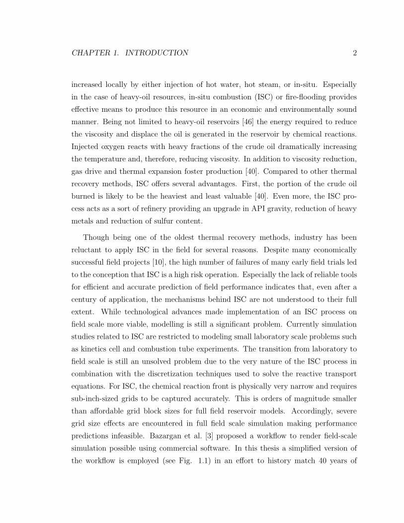
the workflow is employed (see Fig. 1.1) in an effort to history match 40 years of
CHAPTER 1. INTRODUCTION 3
production of one of the worlds largest and most successful ISC projects located in
Central Europe.
Figure 1.1: Simplified workflow from [3] for ISC simulation on field scale.
To establish parameter values for the kinetic models used in the numerical simula-
tion of ISC processes, kinetic cell and combustion tube experiments provide a sound
basis. Kinetic cell experiments help to determine the reaction kinetics that are defined
as the study of rate and extent of chemical transformation of reactants to products
(see Chapter 2). Combustion tube runs help to determine important parameters like
equivalent hydrogen-carbon ratio (H/C ratio) and can give an idea of the stoichiom-
etry for the high temperature oxidation process (see Chapter 3). The parameters
obtained are then used in combustion tube and field-scale simulation respectively.
Combustion tube simulations are not included in this thesis. Chapter 4 summarizes
the steps taken for history matching oil production of a 300,000 cell sector model
including 10 years of cold and 30 years of hot production.
Chapter 2
Kinetic Cell Experiments
Before completing combustion tube runs, it is vital to understand and determine
the reaction kinetics of oxidation of reactants to products. The study of kinetics of
crude-oil oxidation in porous media helps to characterize the reactivity of the oil, to
determine the conditions required to achieve ignition, gain insight into the nature
of fuel formed, and to establish parameter values for the kinetic models used in the
numerical simulation [48].
In order to determine the kinetic parameters of the crude oil (pre-exponential fac-
tor, activation energy), several conventional methods like accelerated rate calorimetry
[48] or thermogravimetric analysis [2] can be used. According to [9] the previously
mentioned methods assume a reaction model to interpret experimental data that may
lead to oversimplification. Kinetic parameters in this case, however, were determined
based on the isoconversional method as described in [56] and applied to crude oil
as shown by [12, 13, 14]. As pointed out in [21] combustion of crude oil in porous
media is not a simple reaction but follows several consecutive and competing reac-
tions occurring through different temperature ranges. In order to model the reactions
that occur in a combustion process, an extended compositional analysis and a large
number of kinetic expressions are required. An accurate description of the oxidation
of the simplest hydrocarbon, methane, requires hundreds of reactions to be taken into
account [48]. A similar level of detail for crude oil appears exceptionally difficult to
develop. The activation energy calculated is apparent, effective, or variable in the
4
CHAPTER 2. KINETIC CELL EXPERIMENTS 5
sense that it is a result of reactions occurring in parallel that are lumped together
into one activation energy value [24, 54]. The isoconversional approach provides a
model-free technique to estimate effective activation energy, is useful for screening of
the likelihood of successful combustion, and suggests the global reactions governing
ISC.
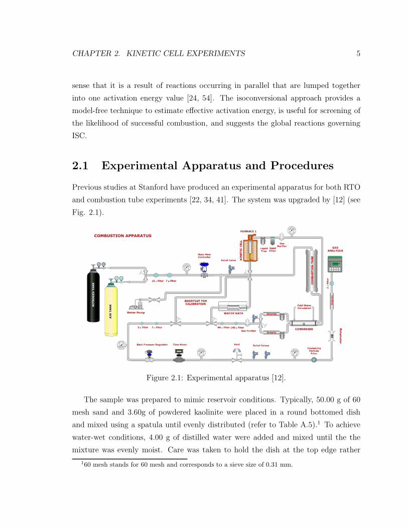
2.1 Experimental Apparatus and Procedures
Previous studies at Stanford have produced an experimental apparatus for both RTO
and combustion tube experiments [22, 34, 41]. The system was upgraded by [12] (see
Fig. 2.1).
Figure 2.1: Experimental apparatus [12].
The sample was prepared to mimic reservoir conditions. Typically, 50.00 g of 60
mesh sand and 3.60g of powdered kaolinite were placed in a round bottomed dish
and mixed using a spatula until evenly distributed (refer to Table A.5).1 To achieve
water-wet conditions, 4.00 g of distilled water were added and mixed until the the
mixture was evenly moist. Care was taken to hold the dish at the top edge rather
160 mesh stands for 60 mesh and corresponds to a sieve size of 0.31 mm.
CHAPTER 2. KINETIC CELL EXPERIMENTS 6
than at the bottom to prevent body heat fostering premature evaporation of water.
Finally, 2.00 g of the crude oil under investigation were added and blended until a
homogeneous mixture was obtained. The crude oil is 15.9 API◦ and 2000 cP at 18◦C.
Then, the sample was tamped into the kinetics cell using a plunger. A coarse 16
mesh sand provided inlet gas distribution.2 With the sample in the kinetic cell, the
end plugs were tightened. To guarantee leak-free operational conditions, the cell was
flushed with nitrogen and the test pressure was gradually increased to approximately
150 psi. The pressurized cell was then submerged in a water bath to check for leaks.
If no leaks were detected, the outside of the cell was dried and placed in the furnace.
Thermocouples are used to measure temperature at three different points along the
center of the cell and in the furnace to check for a uniform temperature distribution.
Before each experiment, all modules (CO2, CO, CH4, and O2) of the gas analyzer
were calibrated using high purity calibration gases. Care was taken to ensure that
each module was subject to its calibration gas for a sufficient time. After the cali-
bration was finished, the cell was pressurized to 100 psia corresponding to reservoir
conditions. Additionally, connections were scrutinized for leaks using a detergent
solution. The experiment was then started. Based on a pre-programmed heating
schedule the temperature was increased linearly while air was passed through the cell
at a flow rate of 2 l/min. The pressure at the inlet and the outlet of the cell, exit flow
rate, temperature in the cell and furnace, and effluent gas composition were recorded
continuously during the experiment.
As outlined in [13], the isoconversional technique requires a series of experiments
to be conducted at different heating rates. All other parameters, such as pressure, flow
rate, and initial temperature are held fixed for all tests. Each experiment is conducted
with great care to achieve satisfactory and consistent results. Some variability does
exist from run to run. For instance, water evaporates during sample preparation and
some oil adheres to the surface of the dish.
216 mesh corresponds to a sieve size of 1.4 mm.

CHAPTER 2. KINETIC CELL EXPERIMENTS 7
2.2 Post-Processing of Experimental Data and Di-
agnostic Plots
During the experiment effluent O2, CO2, and CO are recorded using a gas analyzer.
Gas data cannot be used directly. The isoconversional principle requires conversion
and, therefore, the oxygen consumption to be calculated. The problem is that the
composition of the air used is not exactly 21% oxygen and 79% nitrogen. The oxygen
concentration at the outlet is between 20.5% and 21% when no oxygen is consumed.
Hence, a baseline must be determined not only for oxygen but for all gases measured.
As a best practice, it was decided to determine the baseline by taking an average value
from the gas readings up to one hour into the experiment. Any negative values were
forced to zero. Unfortunately, the gas analyzer readings shift over time suggesting
that oxygen is consumed even after all oil was burned (see Fig. 2.2 after three hours
into the experiment). The variations in initial and final state of oxygen consumption
are compensated by applying a technique originally used for background correction
in X-ray Photoelectron Spectroscopy (XPS) data. In this case, the [52] algorithm is
used to construct a background sensitive to changes in data.
0
0.5
1.0
1.5
2.0
2.5
3.0
3.5
0 0.5 1.0 1.5 2.0 2.5 3.0 3.50
100
200
300
400
500
600
700
MolarFra
ction
(%) T
em
pera
ture
(◦C)
Time (h)
O2 consumed
CO2 produced
CO produced
Temperature @ top of kinetic cell
Temperature @ center of kinetic cell
Temperature @ bottom of kinetic cell
lag between readings
non-zero readings afterfull conversionnegative gas readings,
noisy CO signal
Figure 2.2: Example of RTO kinetics experimental results and measurement issues.
Fig. 2.2 also shows that the individual modules of the gas analyzer have lag
CHAPTER 2. KINETIC CELL EXPERIMENTS 8
0
0.5
1.0
1.5
2.0
2.5
3.0
3.5
0 0.5 1.0 1.5 2.0 2.5 3.0 3.50
100
200
300
400
500
600
700M
olarFra
ction
(%) T
em
pera
ture
(◦C)
Time (h)
O2 consumed
CO2 produced
CO produced
Temperature @ top of kinetic cellLTO
HTO
DeathValley
negative temperaturegradient region
Figure 2.3: Example of corrected RTO kinetics experimental results.
relative to each other because of different types of sensors. The time difference is
especially pronounced for oxygen and carbon dioxide. The carbon dioxide readings
as well as the carbon monoxide readings had to be shifted with respect to oxygen
readings. The carbon dioxide readings were filtered using a finite impulse response
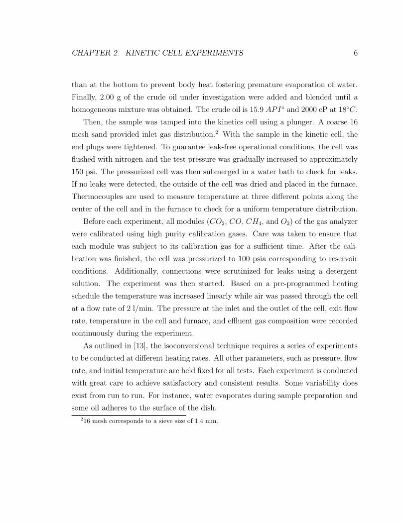
smoothing filter as described in [49]. In Fig. 2.3, the measured data was corrected
using the methods described above. In comparison with Fig. 2.2, Fig. 2.3 shows no
gas production/consumption after the experiment has finished and no lag between
individual gas readings.
The burning behavior of the oil observed in Fig. 2.3 is comparable to other ex-
perimental results reported [6, 13, 35]. In the literature, two main regions are distin-
guished. Generally, low temperature oxidation (LTO) reactions occur below ≈ 350◦C
and are thought of as oxygen addition reactions yielding partially oxygenated com-
pounds [6]. However, as pointed out in [37], the temperature range is oil dependent.
The high temperature oxidation (HTO) reaction is the actual burning or bond-scission
reaction i.e. the reaction between fuel and air injected. This reaction is believed to
happen above 350◦C [44]. LTO and HTO regions are separated by the negative tem-
perature gradient region, also referred to as Death Valley.3 In some cases, however,
3The term was coined by Prof. Gordon Moore at the University of Calgary.

CHAPTER 2. KINETIC CELL EXPERIMENTS 9
LTO and HTO reactions were reported to overlap [1].
A distinctive part of the LTO region is the negative temperature gradient [39].
Although temperature increases, less and less oxygen is consumed. The fuel is then
burned in the HTO region [44]. The sharp peak in oxygen consumption indicates that
an extensive amount of conversion happens for a very small temperature window (from
400◦C to 430◦C). For both, LTO and HTO reactions, an increase in temperature is
observed (see Fig. 2.3). As mentioned before, the temperature is recorded at three
different positions in the kinetic cell i.e. at the bottom of the cell (BOC), center of
the cell (COC), and at the top of the cell (TOC). For the isoconversional analysis,
always, the temperature profile yielding the greatest deviation from the programmed
heating profile is used. Usually this is true for the uppermost thermocouple at the
top of the cell (see Fig. 2.2). It is assumed that the reaction releasing the most heat
is the dominant reaction. Therefore, when calculating effective activation energies,
the profile giving the greatest temperature deviation is used to capture this/these
reaction(s). Also, during the experiment it is assumed that the oil is pushed towards
the upper part of the cell because air is injected from below. A temperature increase
results in a viscosity decrease making it easier for the oil to move.
2.3 Kinetic Cell Results
For kinetic cell runs three different solid mixtures were taken into consideration to
study the effect of surface area. First, experiments were carried out using production
sand. Production sand refers to sand produced along with the oil and collected in
the surface lines. Based on reservoir-core material, the mineralogy was investigated
using X-Ray Diffraction Analysis. The results of these measurements are summarized
in Table A.2 and Table A.3. Notably, the overall clay content is about 20%. The
production sand used for investigation was contaminated with oil and had to be
cleaned first using toluene. After all oil was removed, the sand was put into a vacuum
oven at 38◦C to ensure that all toluene was evaporated. Then, the sand was saturated
with distilled water to re-hydrate any clays present that might have been affected by
the toluene. Again the sand was put into a vacuum oven at 38◦C until dry. Next
CHAPTER 2. KINETIC CELL EXPERIMENTS 10
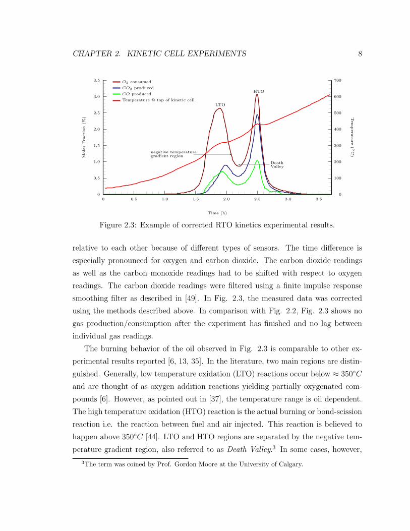
a sieving analysis was carried out using ≈ 580g of cleansed production sand. Sieve
meshes from 14# up to 200# were available. Based on the results a grading curve was
constructed and the diameters D10, D30, and D60 were determined. Furthermore, the
uniformity coefficient Cu and coefficient of curvature Cc were calculated (see Table
A.4). A histogram of the grain size data is given in Fig. 2.4.
14# 16# 20# 42# 60# 80# 100#200# Pan0
5
10
15
20
25
30
35
40
45
50
%on
sievere
tain
ed
Figure 2.4: Histogram for sieve analysis.
Overall the sand shows a bimodal distribution with almost half of the grains having
a size smaller than 0.075 mm. The solid mixture used for the kinetic cell runs shown
in Fig. 2.5 is summarized in Table A.5.
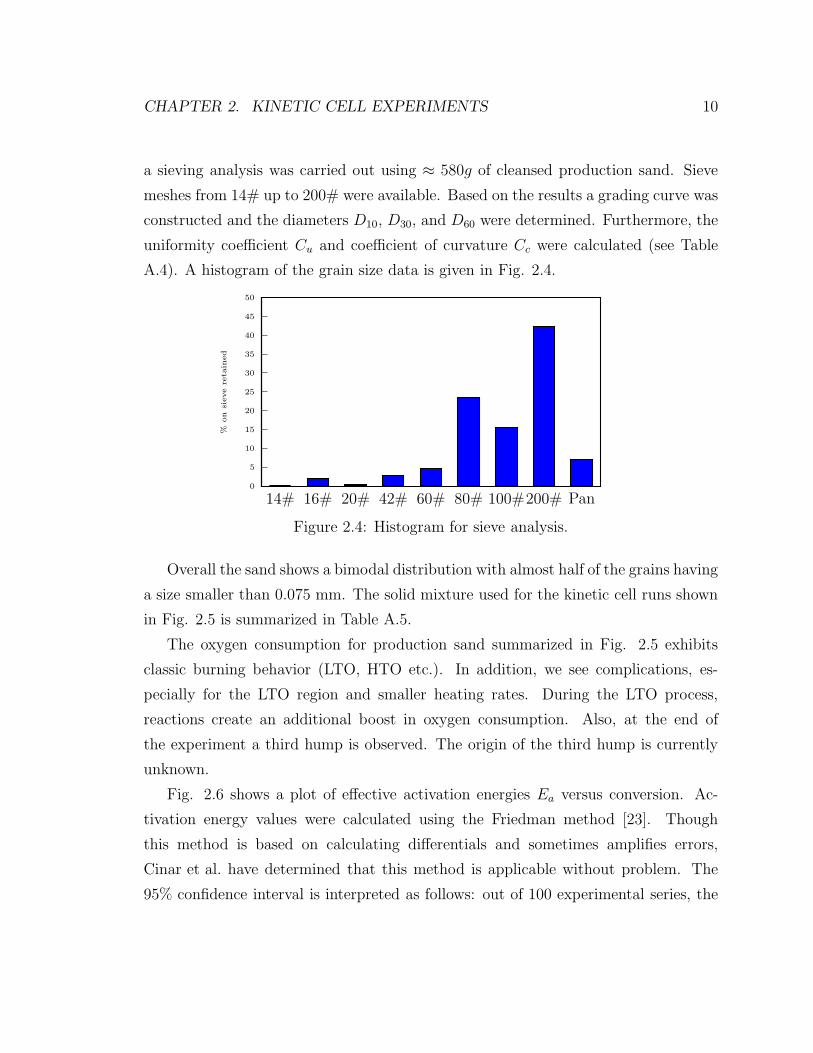
The oxygen consumption for production sand summarized in Fig. 2.5 exhibits
classic burning behavior (LTO, HTO etc.). In addition, we see complications, es-
pecially for the LTO region and smaller heating rates. During the LTO process,
reactions create an additional boost in oxygen consumption. Also, at the end of
the experiment a third hump is observed. The origin of the third hump is currently
unknown.
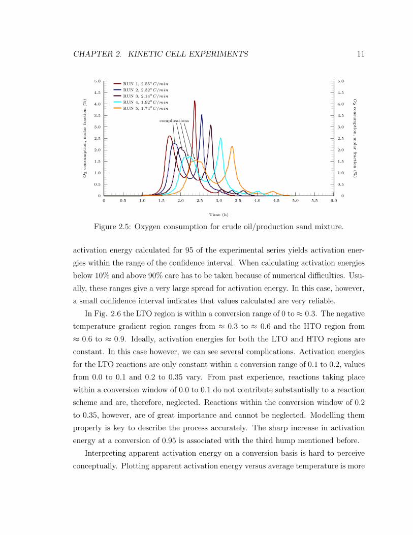
Fig. 2.6 shows a plot of effective activation energies Ea versus conversion. Ac-
tivation energy values were calculated using the Friedman method [23]. Though
this method is based on calculating differentials and sometimes amplifies errors,
Cinar et al. have determined that this method is applicable without problem. The
95% confidence interval is interpreted as follows: out of 100 experimental series, the
CHAPTER 2. KINETIC CELL EXPERIMENTS 11
0
0.5
1.0
1.5
2.0
2.5
3.0
3.5
4.0
4.5
5.0
0 0.5 1.0 1.5 2.0 2.5 3.0 3.5 4.0 4.5 5.0 5.5 6.00
0.5
1.0
1.5
2.0
2.5
3.0
3.5
4.0
4.5
5.0O
2consu
mption,m
olarfraction
(%) O
2consu
mptio
n,m
olarfra
ctio
n(%
)
Time (h)
RUN 1, 2.55◦C/min
RUN 2, 2.32◦C/min
RUN 3, 2.14◦C/min
RUN 4, 1.92◦C/min
RUN 5, 1.74◦C/min
complications
Figure 2.5: Oxygen consumption for crude oil/production sand mixture.
activation energy calculated for 95 of the experimental series yields activation ener-
gies within the range of the confidence interval. When calculating activation energies
below 10% and above 90% care has to be taken because of numerical difficulties. Usu-
ally, these ranges give a very large spread for activation energy. In this case, however,
a small confidence interval indicates that values calculated are very reliable.
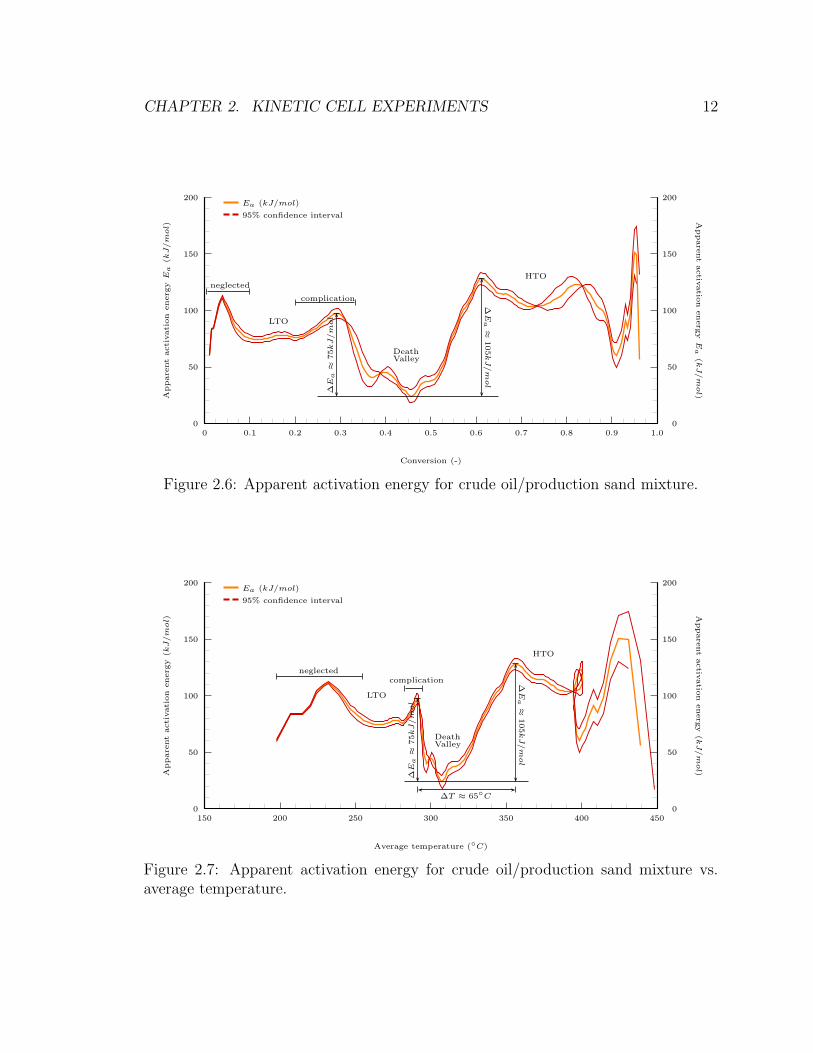
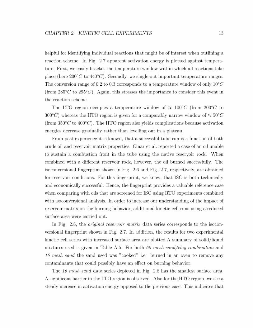
In Fig. 2.6 the LTO region is within a conversion range of 0 to ≈ 0.3. The negative
temperature gradient region ranges from ≈ 0.3 to ≈ 0.6 and the HTO region from
≈ 0.6 to ≈ 0.9. Ideally, activation energies for both the LTO and HTO regions are
constant. In this case however, we can see several complications. Activation energies
for the LTO reactions are only constant within a conversion range of 0.1 to 0.2, values
from 0.0 to 0.1 and 0.2 to 0.35 vary. From past experience, reactions taking place
within a conversion window of 0.0 to 0.1 do not contribute substantially to a reaction
scheme and are, therefore, neglected. Reactions within the conversion window of 0.2
to 0.35, however, are of great importance and cannot be neglected. Modelling them
properly is key to describe the process accurately. The sharp increase in activation
energy at a conversion of 0.95 is associated with the third hump mentioned before.
Interpreting apparent activation energy on a conversion basis is hard to perceive
conceptually. Plotting apparent activation energy versus average temperature is more
CHAPTER 2. KINETIC CELL EXPERIMENTS 12
0
50
100
150
200
0 0.1 0.2 0.3 0.4 0.5 0.6 0.7 0.8 0.9 1.00
50
100
150
200
Appare
ntactivation
energ
yE
a(k
J/m
ol)
Appare
ntactiv
atio
nenerg
yE
a(k
J/m
ol)
Conversion (-)
Ea (kJ/mol)
95% confidence interval
LTO
HTO
DeathValley
neglected
complication
∆E
a≈
105kJ/m
ol
∆E
a≈
75kJ/m
ol
Figure 2.6: Apparent activation energy for crude oil/production sand mixture.
0
50
100
150
200
150 200 250 300 350 400 4500
50
100
150
200
Appare
ntactivation
energ
y(k
J/m
ol)
Appare
ntactiv
atio
nenerg
y(k
J/m
ol)
Average temperature (◦C)
Ea (kJ/mol)
95% confidence interval
LTO
HTO
DeathValley
neglectedcomplication
∆T ≈ 65◦C
∆E
a≈
105kJ/m
ol
∆E
a≈
75kJ/m
ol
Figure 2.7: Apparent activation energy for crude oil/production sand mixture vs.average temperature.
CHAPTER 2. KINETIC CELL EXPERIMENTS 13
helpful for identifying individual reactions that might be of interest when outlining a
reaction scheme. In Fig. 2.7 apparent activation energy is plotted against tempera-
ture. First, we easily bracket the temperature window within which all reactions take
place (here 200◦C to 440◦C). Secondly, we single out important temperature ranges.
The conversion range of 0.2 to 0.3 corresponds to a temperature window of only 10◦C
(from 285◦C to 295◦C). Again, this stresses the importance to consider this event in
the reaction scheme.
The LTO region occupies a temperature window of ≈ 100◦C (from 200◦C to
300◦C) whereas the HTO region is given for a comparably narrow window of ≈ 50◦C
(from 350◦C to 400◦C). The HTO region also yields complications because activation
energies decrease gradually rather than levelling out in a plateau.
From past experience it is known, that a successful tube run is a function of both
crude oil and reservoir matrix properties. Cinar et al. reported a case of an oil unable
to sustain a combustion front in the tube using the native reservoir rock. When
combined with a different reservoir rock, however, the oil burned successfully. The
isoconversional fingerprint shown in Fig. 2.6 and Fig. 2.7, respectively, are obtained
for reservoir conditions. For this fingerprint, we know, that ISC is both technically
and economically successful. Hence, the fingerprint provides a valuable reference case
when comparing with oils that are screened for ISC using RTO experiments combined
with isoconversional analysis. In order to increase our understanding of the impact of
reservoir matrix on the burning behavior, additional kinetic cell runs using a reduced
surface area were carried out.
In Fig. 2.8, the original reservoir matrix data series corresponds to the isocon-
versional fingerprint shown in Fig. 2.7. In addition, the results for two experimental
kinetic cell series with increased surface area are plotted.A summary of solid/liquid
mixtures used is given in Table A.5. For both 60 mesh sand/clay combination and
16 mesh sand the sand used was ”cooked” i.e. burned in an oven to remove any
contaminants that could possibly have an effect on burning behavior.
The 16 mesh sand data series depicted in Fig. 2.8 has the smallest surface area.
A significant barrier in the LTO region is observed. Also for the HTO region, we see a
steady increase in activation energy opposed to the previous case. This indicates that
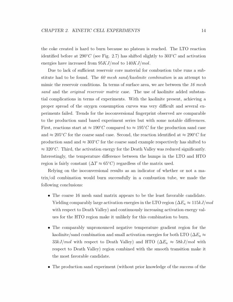
CHAPTER 2. KINETIC CELL EXPERIMENTS 14
the coke created is hard to burn because no plateau is reached. The LTO reaction
identified before at 290◦C (see Fig. 2.7) has shifted slightly to 303◦C and activation
energies have increased from 95KJ/mol to 140KJ/mol.
Due to lack of sufficient reservoir core material for combustion tube runs a sub-
stitute had to be found. The 60 mesh sand/kaolinite combination is an attempt to
mimic the reservoir conditions. In terms of surface area, we are between the 16 mesh
sand and the original reservoir matrix case. The use of kaolinite added substan-
tial complications in terms of experiments. With the kaolinite present, achieving a
proper spread of the oxygen consumption curves was very difficult and several ex-
periments failed. Trends for the isoconversional fingerprint observed are comparable
to the production sand based experiment series but with some notable differences.
First, reactions start at ≈ 190◦C compared to ≈ 195◦C for the production sand case
and ≈ 205◦C for the coarse sand case. Second, the reaction identified at ≈ 290◦C for
production sand and ≈ 303◦C for the coarse sand example respectively has shifted to
≈ 320◦C. Third, the activation energy for the Death Valley was reduced significantly.
Interestingly, the temperature difference between the humps in the LTO and HTO
region is fairly constant (∆T ≈ 65◦C) regardless of the matrix used.
Relying on the isoconversional results as an indicator of whether or not a ma-
trix/oil combination would burn successfully in a combustion tube, we made the
following conclusions:
• The coarse 16 mesh sand matrix appears to be the least favorable candidate.
Yielding comparably large activation energies in the LTO region (∆Ea ≈ 115kJ/mol
with respect to Death Valley) and continuously increasing activation energy val-
ues for the HTO region make it unlikely for this combination to burn.
• The comparably unpronounced negative temperature gradient region for the
kaolinite/sand combination and small activation energies for both LTO (∆Ea ≈
33kJ/mol with respect to Death Valley) and HTO (∆Ea ≈ 58kJ/mol with
respect to Death Valley) region combined with the smooth transition make it
the most favorable candidate.
• The production sand experiment (without prior knowledge of the success of the
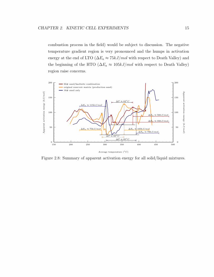
CHAPTER 2. KINETIC CELL EXPERIMENTS 15
combustion process in the field) would be subject to discussion. The negative
temperature gradient region is very pronounced and the humps in activation
energy at the end of LTO (∆Ea ≈ 75kJ/mol with respect to Death Valley) and
the beginning of the HTO (∆Ea ≈ 105kJ/mol with respect to Death Valley)
region raise concerns.
0
50
100
150
200
150 200 250 300 350 400 450 5000
50
100
150
200
Appare
ntactivation
energ
y(k
J/m
ol)
Appare
ntactiv
atio
nenerg
y(k
J/m
ol)
Average temperature (◦C)
60# sand/kaolinite combination
original reservoir matrix (production sand)
16# sand only
∆Ea ≈ 75kJ/mol ∆Ea ≈ 105kJ/mol
∆Ea ≈ 115kJ/mol
∆Ea ≈ 78kJ/mol
∆Ea ≈ 58kJ/mol
∆Ea ≈ 33kJ/mol
∆T ≈ 65◦C
∆T ≈ 65◦C
∆T ≈ 62◦C
Figure 2.8: Summary of apparent activation energy for all solid/liquid mixtures.
Chapter 3
Combustion Tube Experiments
As pointed out in [43], combustion tube runs are not scaled experiments and act as a
proxy for a differential element of a reservoir. When designing tube runs, heat losses
are a major concern. The heat losses for tubes are due to the metal construction and
cannot be compared with the heat losses resulting from the over- and underburden
of the reservoir. In fact over- and underburden heat losses are generally small in
comparison to experiments. Even after a combustion project has finished, the vast
amount of heat stored in the reservoir is still observed after several years. To overcome
heat losses, and prevent a premature termination of the combustion front, the tube
was insulated using an aerogel based material.1 Furthermore, the air flux is sufficiently
large to sustain the combustion front.
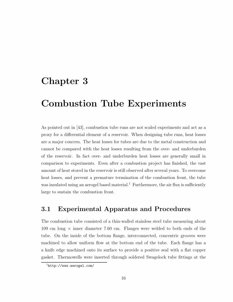
3.1 Experimental Apparatus and Procedures
The combustion tube consisted of a thin-walled stainless steel tube measuring about
109 cm long × inner diameter 7.60 cm. Flanges were welded to both ends of the
tube. On the inside of the bottom flange, interconnected, concentric grooves were
machined to allow uniform flow at the bottom end of the tube. Each flange has a
a knife edge machined onto its surface to provide a positive seal with a flat copper
gasket. Thermowells were inserted through soldered Swagelock tube fittings at the
1http://www.aerogel.com/
16
CHAPTER 3. COMBUSTION TUBE EXPERIMENTS 17
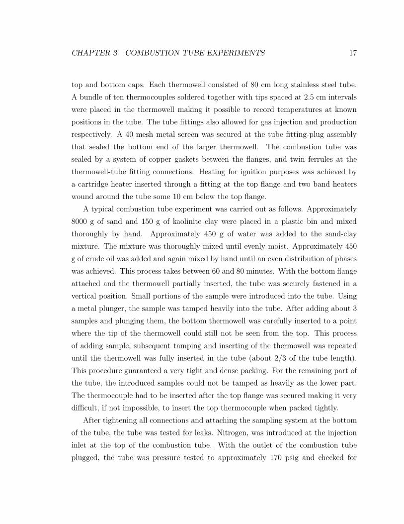
top and bottom caps. Each thermowell consisted of 80 cm long stainless steel tube.
A bundle of ten thermocouples soldered together with tips spaced at 2.5 cm intervals
were placed in the thermowell making it possible to record temperatures at known
positions in the tube. The tube fittings also allowed for gas injection and production
respectively. A 40 mesh metal screen was secured at the tube fitting-plug assembly
that sealed the bottom end of the larger thermowell. The combustion tube was
sealed by a system of copper gaskets between the flanges, and twin ferrules at the
thermowell-tube fitting connections. Heating for ignition purposes was achieved by
a cartridge heater inserted through a fitting at the top flange and two band heaters
wound around the tube some 10 cm below the top flange.
A typical combustion tube experiment was carried out as follows. Approximately
8000 g of sand and 150 g of kaolinite clay were placed in a plastic bin and mixed
thoroughly by hand. Approximately 450 g of water was added to the sand-clay
mixture. The mixture was thoroughly mixed until evenly moist. Approximately 450
g of crude oil was added and again mixed by hand until an even distribution of phases
was achieved. This process takes between 60 and 80 minutes. With the bottom flange
attached and the thermowell partially inserted, the tube was securely fastened in a
vertical position. Small portions of the sample were introduced into the tube. Using
a metal plunger, the sample was tamped heavily into the tube. After adding about 3
samples and plunging them, the bottom thermowell was carefully inserted to a point
where the tip of the thermowell could still not be seen from the top. This process
of adding sample, subsequent tamping and inserting of the thermowell was repeated
until the thermowell was fully inserted in the tube (about 2/3 of the tube length).
This procedure guaranteed a very tight and dense packing. For the remaining part of
the tube, the introduced samples could not be tamped as heavily as the lower part.
The thermocouple had to be inserted after the top flange was secured making it very
difficult, if not impossible, to insert the top thermocouple when packed tightly.
After tightening all connections and attaching the sampling system at the bottom
of the tube, the tube was tested for leaks. Nitrogen, was introduced at the injection
inlet at the top of the combustion tube. With the outlet of the combustion tube
plugged, the tube was pressure tested to approximately 170 psig and checked for

CHAPTER 3. COMBUSTION TUBE EXPERIMENTS 18
leaks. After depressurizing, the tube was insulated as described in [30].
Overnight the tube was stored in a horizontal position to reduce gravity drainage
effects. The next day the tube was secured in a vertical position, all tubes and
sensors were hooked up, the gas analyzer calibrated and nitrogen injection started.
The gas injection rate was set on the mass flow controller at approximately 2 l/min.
The back-pressure regulator was adjusted to obtain an injection pressure of about
100 psig. Electric current was introduced into the heater cartridge and the band
heaters in gradual steps using a variable power transformer. When the temperature
in the combustion tube at the heater thermocouple reached approximately 500 ◦C,
air injection was initiated and the power to the heating devices was gradually reduced
over a time frame of 30 to 45 minutes. The air injection rate was set to 3 l/min. During
most of the experiments the back-pressure regulator was adjusted for an injection
pressure of 100 psig to obtain reservoir conditions. In some special cases the pressure
was not adjusted. The pressure of the tube, exit flow rate, temperature, and effluent
gas composition were recorded continuously during the experiment.
Typically right after air injection began, a dramatic rise in temperature was ob-
served. For most cases water production started after 2.5 hours, whereas oil pro-
duction started after 4 hours after ignition. Produced liquids were collected in the
sample system. Due to the initially undersized sampling system, the liquids had to
be collected from the sampling bomb into graduated sample bottles that were tightly
capped for subsequent analysis. For safety reasons the sand pack was was not burned
to the bottom flange and combustion was stopped about 25 cm above the bottom
flange by flushing the tube with nitrogen at a flow rate of 3 l/min. A typical run
required between 4 to 6 hours of air injection depending on flow rate. Overnight, the
tube was left in a vertical position to let oil drain and for cooling.
The next day, the setup was dismantled and a post mortem analysis was per-
formed. During the post mortem analysis the remains of the sand pack were collected,
categorized, and weighed. This helped to provide information on the axial profile in
terms of coke, water, and extractable oil.
CHAPTER 3. COMBUSTION TUBE EXPERIMENTS 19
3.2 Experimental Data Collected
Physical data obtained automatically from combustion tube runs are as follows:
• Effluent CO2, CO, CH4 and O2 concentration.
• Temperature measurements from along the tube, 20 individual measurements
in total.
As in the case of the kinetic cell, data are not used directly. Again care has
to be taken for the lag introduced by the gas analyzer, as well as the lag between
temperature readings and gas measurements. Fig. 3.1 and Fig. 3.2 show the the gas
and temperature readings of the first combustion tube run. The matrix and liquid
composition used in this case is summarized in Table A.6. In terms of composition
this setup corresponds to the kinetic cell run using fine sand and clay (see Fig. 2.8
for activation energies and Table A.5 for oil, water, sand, and clay proportions).
0
1
2
3
4
5
6
7
8
9
10
11
12
13
14
15
16
0 1 2 3 4 5 6 7 80
1
2
3
4
5
6
7
8
9
10
11
12
13
14
15
16
MolarFra
ction
(%) M
olarFra
ctio
n(%
)
Time (h)
O2 excess
CO2 produced
CO produced
CH4 produced
N2 injection
SamplingSpikesOscillations
Start O2
InjectionFlush N2
Start CH4
distillation
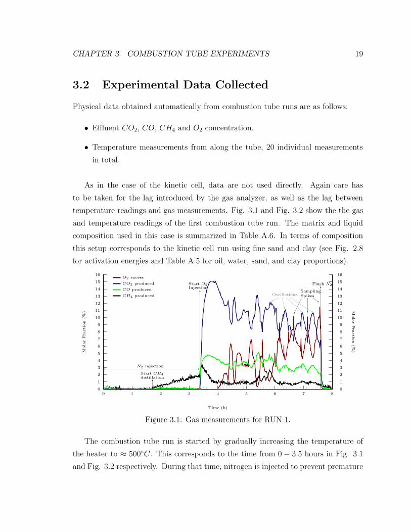
Figure 3.1: Gas measurements for RUN 1.
The combustion tube run is started by gradually increasing the temperature of
the heater to ≈ 500◦C. This corresponds to the time from 0 − 3.5 hours in Fig. 3.1
and Fig. 3.2 respectively. During that time, nitrogen is injected to prevent premature
CHAPTER 3. COMBUSTION TUBE EXPERIMENTS 20
0
100
200
300
400
500
600
0 1 2 3 4 5 6 7 80
100
200
300
400
500
600Tem
pera
ture
(◦C) T
em
pera
ture
(◦C)
Time (h)
Heater thermocouple
Thermocouple 1
Thermocouple n
Thermocouple 20
N2 injection
Start O2
Injection Overheating
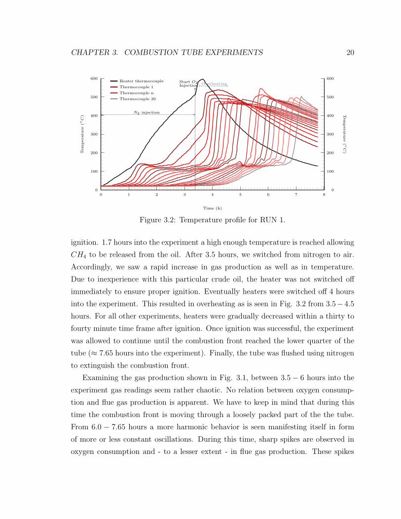
Figure 3.2: Temperature profile for RUN 1.
ignition. 1.7 hours into the experiment a high enough temperature is reached allowing
CH4 to be released from the oil. After 3.5 hours, we switched from nitrogen to air.
Accordingly, we saw a rapid increase in gas production as well as in temperature.
Due to inexperience with this particular crude oil, the heater was not switched off
immediately to ensure proper ignition. Eventually heaters were switched off 4 hours
into the experiment. This resulted in overheating as is seen in Fig. 3.2 from 3.5− 4.5
hours. For all other experiments, heaters were gradually decreased within a thirty to
fourty minute time frame after ignition. Once ignition was successful, the experiment
was allowed to continue until the combustion front reached the lower quarter of the
tube (≈ 7.65 hours into the experiment). Finally, the tube was flushed using nitrogen
to extinguish the combustion front.
Examining the gas production shown in Fig. 3.1, between 3.5− 6 hours into the
experiment gas readings seem rather chaotic. No relation between oxygen consump-
tion and flue gas production is apparent. We have to keep in mind that during this
time the combustion front is moving through a loosely packed part of the the tube.
From 6.0 − 7.65 hours a more harmonic behavior is seen manifesting itself in form
of more or less constant oscillations. During this time, sharp spikes are observed in
oxygen consumption and - to a lesser extent - in flue gas production. These spikes
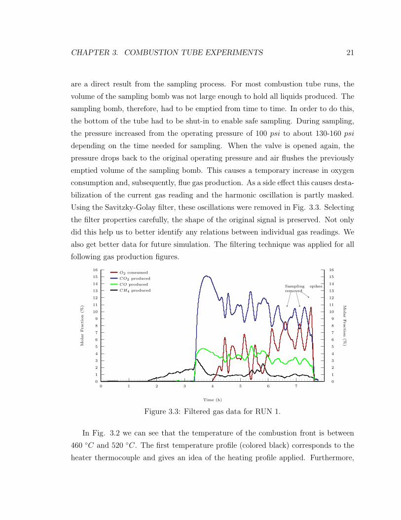
CHAPTER 3. COMBUSTION TUBE EXPERIMENTS 21
are a direct result from the sampling process. For most combustion tube runs, the
volume of the sampling bomb was not large enough to hold all liquids produced. The
sampling bomb, therefore, had to be emptied from time to time. In order to do this,
the bottom of the tube had to be shut-in to enable safe sampling. During sampling,
the pressure increased from the operating pressure of 100 psi to about 130-160 psi
depending on the time needed for sampling. When the valve is opened again, the
pressure drops back to the original operating pressure and air flushes the previously
emptied volume of the sampling bomb. This causes a temporary increase in oxygen
consumption and, subsequently, flue gas production. As a side effect this causes desta-
bilization of the current gas reading and the harmonic oscillation is partly masked.
Using the Savitzky-Golay filter, these oscillations were removed in Fig. 3.3. Selecting
the filter properties carefully, the shape of the original signal is preserved. Not only
did this help us to better identify any relations between individual gas readings. We
also get better data for future simulation. The filtering technique was applied for all
following gas production figures.
0
1
2
3
4
5
6
7
8
9
10
11
12
13
14
15
16
0 1 2 3 4 5 6 70
1
2
3
4
5
6
7
8
9
10
11
12
13
14
15
16
MolarFra
ction
(%) M
olarFra
ctio
n(%
)
Time (h)
O2 consumed
CO2 produced
CO produced
CH4 producedSampling spikesremoved
Figure 3.3: Filtered gas data for RUN 1.
In Fig. 3.2 we can see that the temperature of the combustion front is between
460 ◦C and 520 ◦C. The first temperature profile (colored black) corresponds to the
heater thermocouple and gives an idea of the heating profile applied. Furthermore,
CHAPTER 3. COMBUSTION TUBE EXPERIMENTS 22
we can clearly see the steam plateau around 110◦C during the initial response of each
thermocouple. The temperature for the steam plateau is not constant because we
have to take changing partial pressures into account. Also the sampling process, as
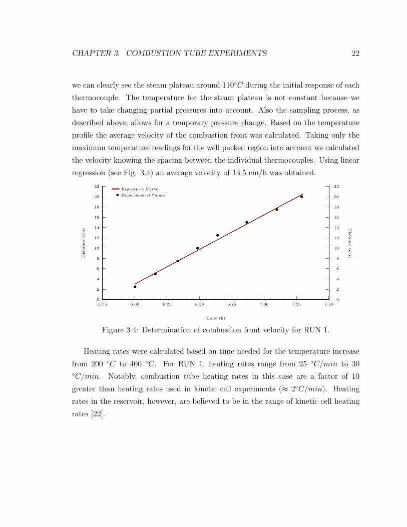
described above, allows for a temporary pressure change. Based on the temperature
profile the average velocity of the combustion front was calculated. Taking only the
maximum temperature readings for the well packed region into account we calculated
the velocity knowing the spacing between the individual thermocouples. Using linear
regression (see Fig. 3.4) an average velocity of 13.5 cm/h was obtained.
b
b
b
b
b
b
b
b
0
2
4
6
8
10
12
14
16
18
20
22
5.75 6.00 6.25 6.50 6.75 7.00 7.25 7.500
2
4
6
8
10
12
14
16
18
20
22
Dista
nce(c
m) D
istance(c
m)
Time (h)
Regression Curve
Experimental Valuesb
Figure 3.4: Determination of combustion front velocity for RUN 1.
Heating rates were calculated based on time needed for the temperature increase
from 200 ◦C to 400 ◦C. For RUN 1, heating rates range from 25 ◦C/min to 30◦C/min. Notably, combustion tube heating rates in this case are a factor of 10
greater than heating rates used in kinetic cell experiments (≈ 2◦C/min). Heating
rates in the reservoir, however, are believed to be in the range of kinetic cell heating
rates [22].
CHAPTER 3. COMBUSTION TUBE EXPERIMENTS 23
3.3 Production Data and Post Mortem
The basic mixture used for a combustion tube run consisted of sand, powdered kaoli-
nite, water and oil (see Table A.6). The actual reservoir properties could not be
matched quantitatively for several reasons. First, an assumed initial oil saturation of
85% would have overloaded the production vessel. Second, at the time the combustion
tube runs were carried out, no general consensus about the amount and type of clay
existed (see Table A.3). Given that all kinetic cell runs were made using kaolinite,
it was decided to continue using this type of clay to mimic an increased surface area
and account for any catalytic effect. In order to make tube runs comparable with
tube runs from previous studies the range for clay in terms of weight percent was set
to a range of [1.8-2.0], the range for oil and water was set to a range of [5.0-6.0].
Water production started between two and four hours after ignition. The pro-
duction vessel had no window so it was not possible to determine the exact start of
water production. As mentioned above during the sampling process, the tube was
shut-in and water and/or oil was released. This continuous sampling process proved
to have several disadvantages. Due to the great pressure drop, liquids could easily
be spilled or evaporated. Also the constant opening and closing of the production
vessel fostered the movement of fines, ending up in the production part of the assem-
bly. This is also one of the reasons why values in Table A.6 do not add up exactly
with production data and weighing results of post mortem analysis. Total production
data as shown in Table A.13 does not give absolute values. It serves as an accurate
estimate of actual production data.
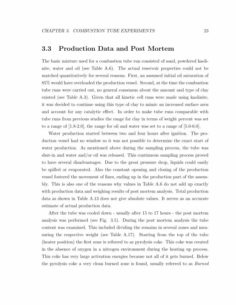
After the tube was cooled down - usually after 15 to 17 hours - the post mortem
analysis was performed (see Fig. 3.5). During the post mortem analysis the tube
content was examined. This included dividing the remains in several zones and mea-
suring the respective weight (see Table A.17). Starting from the top of the tube
(heater position) the first zone is referred to as pyrolysis coke. This coke was created
in the absence of oxygen in a nitrogen environment during the heating up process.
This coke has very large activation energies because not all of it gets burned. Below
the pyrolysis coke a very clean burned zone is found, usually referred to as Burned
CHAPTER 3. COMBUSTION TUBE EXPERIMENTS 24
Figure 3.5: Post mortem for RUN 1 (weighing results given in Table A.17).
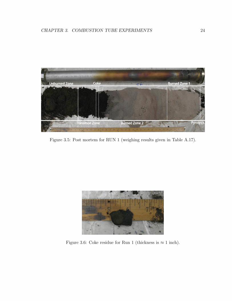
Figure 3.6: Coke residue for Run 1 (thickness is ≈ 1 inch).
CHAPTER 3. COMBUSTION TUBE EXPERIMENTS 25
Zone 1. Below Burned Zone 1, Burned Zone 2 is found. There are two main rea-
sons why Burned Zone 1 is cleaner (or lighter visually speaking). First, this zone
was subject to the heater cartridge and the band heaters. Therefore, more energy
was available once the tube was ignited and the burning process was more complete.
Second, the upper part of the tube was less compacted for reasons mentioned in the
previous section. For all runs, the observation could be made that the burned zone in
the well packed part of the tube was darker than the burned zone in the not so well
packed part of the tube. This is easy to understand because apparently more oil was
available in the lower part of the tube. Also, it can be assumed that the permeability
of the upper part of the tube is greater compared to the permeability of the lower
part of the tube. Again, and indicator that for a successful field run, the reservoir
permeability has to be reasonably high.
The next zone represents a snapshot of the combustion front where HTO reactions
took place. It has to be kept in mind though, that this is not how the real combustion
front appears. Once the tube run was finished and nitrogen injection was commenced
cracking reactions etc. are still going on because the tube cannot be cooled down
instantly. The thickness of the coke ranged from 0.5 to 2 inches (see Fig. 3.6). The
next zone was a transition zone were cracking and LTO reactions started to take
place. Finally, we have the unburned zone which basically represents the oil bank.
3.4 Stoichiometry
According to [4], the combustion stoichiometry for HTO is expressed as:
CHn +1
Y
(
2m+ 1
2m+ 2+
n
4
)
O2 +R
Y
(
2m+ 1
2m+ 2+
n
4
)
N2 −→
m
m+ 1CO2 +
1
m+ 1CO +
1− Y
Y
(
2m+ 1
2m+ 2+
n
4
)
O2
+n
2H2O +
R
Y
(
2m+ 1
2m+ 2+
n
4
)
N2 (3.1)
The stoichiometric coefficients can be calculated based on normalized gas composition
CHAPTER 3. COMBUSTION TUBE EXPERIMENTS 26
i.e. taking only O2, CO2, and CO of effluent gas analysis into account [8, 48]. In Eq.
3.1, m is the molar ratio of CO over CO2 and R is referred to as the ratio of the mole
fraction of nitrogen to oxygen in the feed gas i.e.
R =
(
YN2
YO2
)
Feed Gas
(3.2)
n stands for the equivalent atomic H/C ratio of the fuel burned. It is important
to point out, that the H/C Ratio only characterizes the HTO reactions. It does
not represent the composition of the fuel actually burned in the combustion tube
because of the LTO reactions that occur in the tube at temperatures below 350◦C
[44]. The effluent gas measured is a result of both LTO and HTO reactions. In terms
of normalized gas composition, n is given with
n =4(
N2
R− CO2 −
CO2
2 −O2
)
CO2 + CO(3.3)
Based on effluent gas data from RUN 1 and using average values for the stabilized
region, the following stoichiometry for the HTO reaction was obtained:
CH1.25 + 1.48O2 + 5.67N2 −→
0.75CO2 + 0.25CO + 0.29O2 + 0.63H2O + 5.67N2 (3.4)
Given that the H/C ratio of the original oil is estimated to be 1.7 and the H/C
ratio of the fuel is 1.25 we conclude from the H/C ratio reduction, that high tem-
perature oxidation was the main oxidation mechanism i.e. most of the oxidation
reactions happened in the HTO region [48]. Butler and Sarathi list several other
important parameters commonly referred to as gas-phase parameters. Among them
is the oxygen-fuel ratio (OFR) that is described as the minimum volume of oxygen
required to burn a unit mass of fuel that has an equivalent atomic H/C ratio given
CHAPTER 3. COMBUSTION TUBE EXPERIMENTS 27
by n. The OFR is believed to be directly proportional to the degree of LTO occurring
in the combustion tube. As mentioned above, during LTO some fraction of the con-
sumed oxygen reacts with the crude oil without generating any of the carbon oxides
or water. The air-fuel ratio (AFR) refers to the volume of air required to burn a unit
mass of fuel. It is of great value when designing a field project. During a combustion
tube run some fraction of the consumed oxygen reacts with oil to form oxygenated
compounds commonly referred to as fO2R. This is especially true for LTO. According
to [48] calculating the fraction of reacted oxygen converted to carbon dioxides gives
an idea to which extent LTO reactions occur in the combustion tube. The results for
RUN 1 (and all other runs) in terms of gas phase parameters for the stabilized region
based on mean values are summarized in Table A.16.
In addition to calculating single values for the stabilized region it is also very
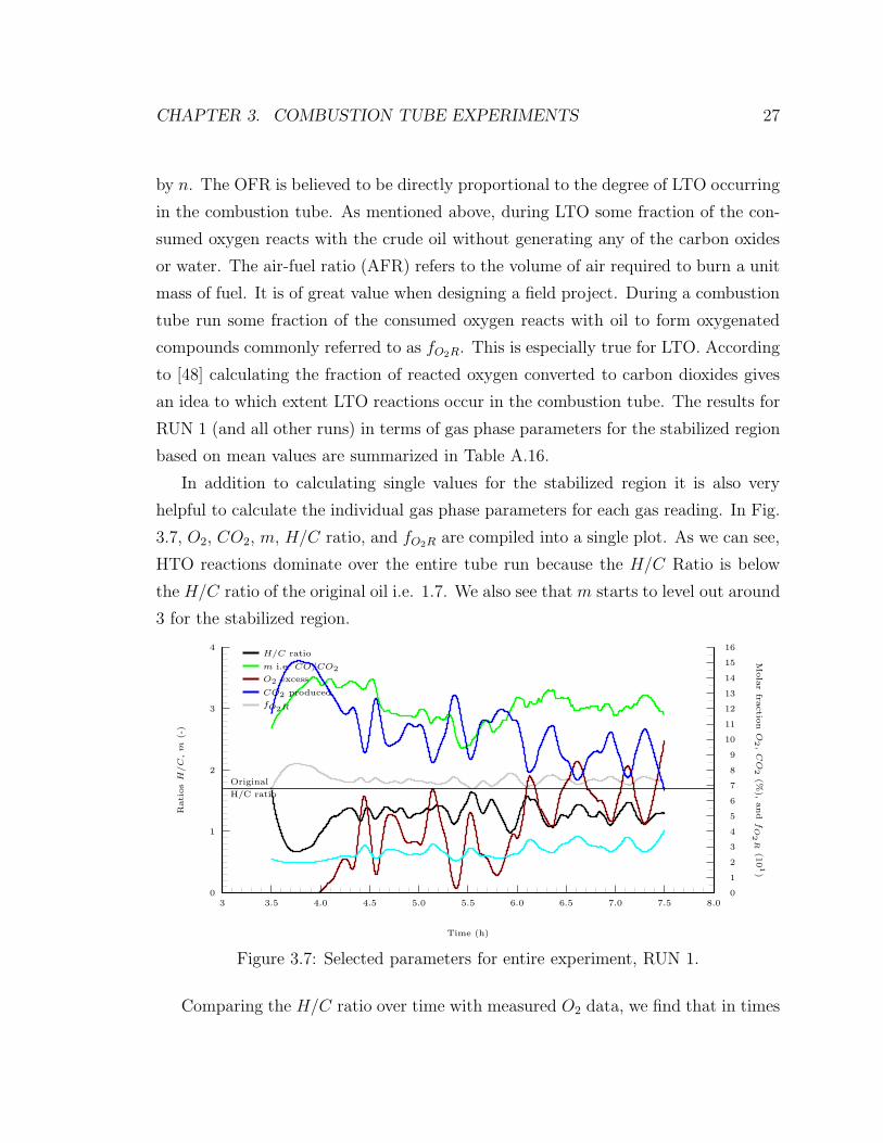
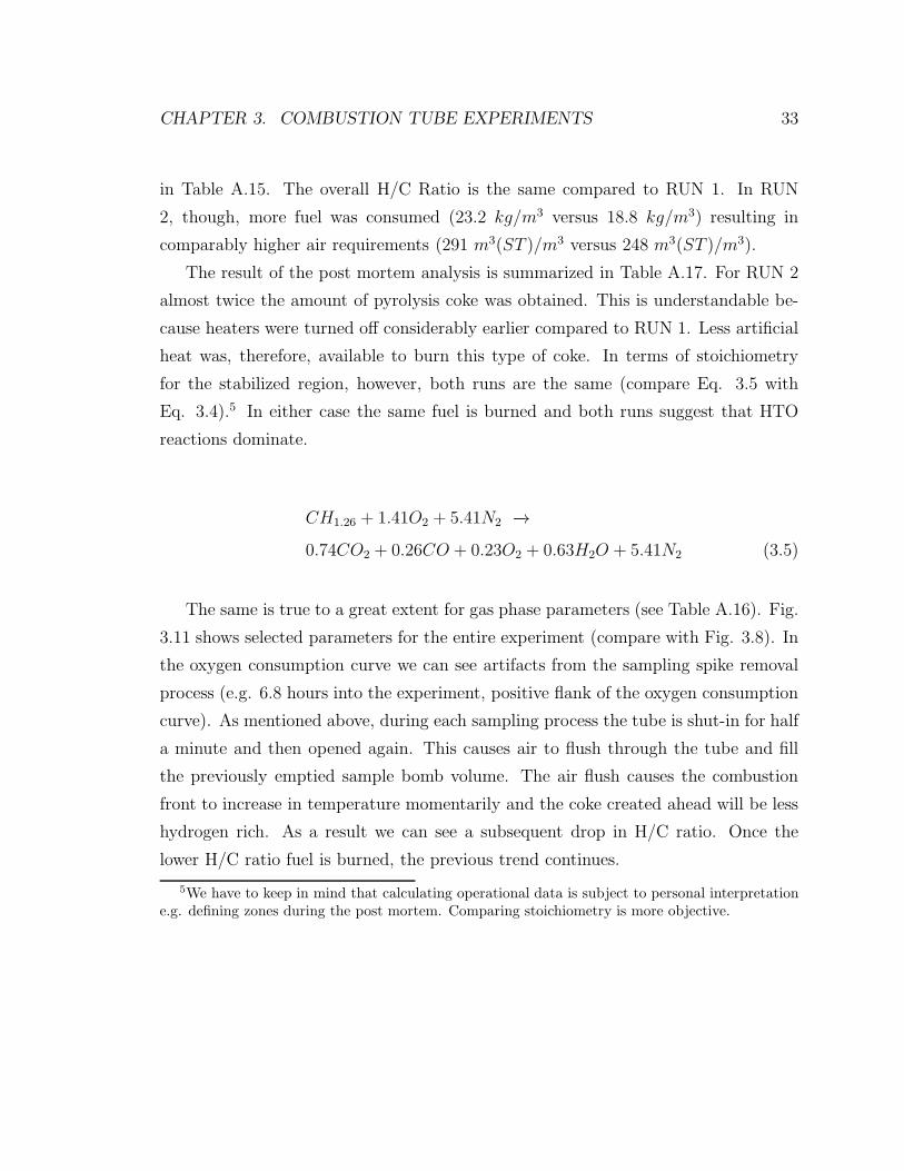
helpful to calculate the individual gas phase parameters for each gas reading. In Fig.
3.7, O2, CO2, m, H/C ratio, and fO2R are compiled into a single plot. As we can see,
HTO reactions dominate over the entire tube run because the H/C Ratio is below
the H/C ratio of the original oil i.e. 1.7. We also see that m starts to level out around
3 for the stabilized region.
0
1
2
3
4
3 3.5 4.0 4.5 5.0 5.5 6.0 6.5 7.0 7.5 8.00
1
2
3
4
5
6
7
8
9
10
11
12
13
14
15
16
RatiosH
/C,m
(-)
Molarfra
ctio
nO
2,CO
2(%
),and
fO
2R
(101)
Time (h)
H/C ratio
m i.e. CO/CO2
O2 excess
CO2 produced
fO2R
Original
H/C ratio
Figure 3.7: Selected parameters for entire experiment, RUN 1.
Comparing the H/C ratio over time with measured O2 data, we find that in times
CHAPTER 3. COMBUSTION TUBE EXPERIMENTS 28
of less oxygen consumption a comparably larger H/C ratio is observed. Given that
fO2R is an indicator to the extent which LTO reactions occur in the combustion tube,
it appears, that a greater H/C ratio also corresponds with a greater amount of LTO
reactions. This periodic change from less oxygen consumption, greater H/C ratio,
and smaller fO2R, to greater oxygen consumption, smaller H/C ratio, and greater
fO2R is especially true for the stabilized region. These oscillations have been mainly
attributed to geomechanical i.e. packing issues, meaning bulk density differences
arising from the packing procedure used for combustion tube preparation [30]. In
this case, however, oscillations cannot be attributed solely to packing issues. This
is particularly true for the lower part of the combustion tube. The packing proce-
dure described above guarantees a homogeneous medium to a great extent. In order
to blame packing for oscillations the frequency of the oscillations has to be related
physically to the packing process.
Let us assume the following. Filling a combustion tube takes roughly 90 scoops of
sample, each scoop weighing about 100 g. Each scoop is consolidated using a metal
plunger. Accordingly, 90 layers of different density are created. Each layer being
about 1.2 cm thick. This is what is referred to as inhomogeneous packing. Given
that the combustion front moves at a velocity of 13.5 cm/h, the front passes around
eleven different layers in one hour. If each layer gives a peak the distance between
the amplitudes is about 1.2 cm which equals to half a period. Consequently it takes
the combustion front 0.18 h to travel a full period. The resulting frequency of the
signal is then around 5.6 Hz. The frequency of the oscillations for the unstabilized
zone from 4.5 to 6 hours in Fig 3.7 is around 7.9× 10⁻⁴ Hz. For the stabilized zone
(from 6 to 7.5 hours), it is even less with 5.6 × 10⁻⁴ Hz and remarkably constant
(compare with RUN 2). To conclude, the frequency observed is too low to be related
to packing.
A more general explanation could be as follows. Looking at Fig. 3.22 on page 43
the amplitude of the oscillations seems to be affected by the flow rate. The lower the
flow rate (see Fig. 3.20), the lower the amplitude of the oscillations. Also, the lower
the flow rate, the lower the frequency of the oscillations. As mentioned before, a
maximum in excess O2 corresponds to a minimum in CO2 production and vice versa.
CHAPTER 3. COMBUSTION TUBE EXPERIMENTS 29
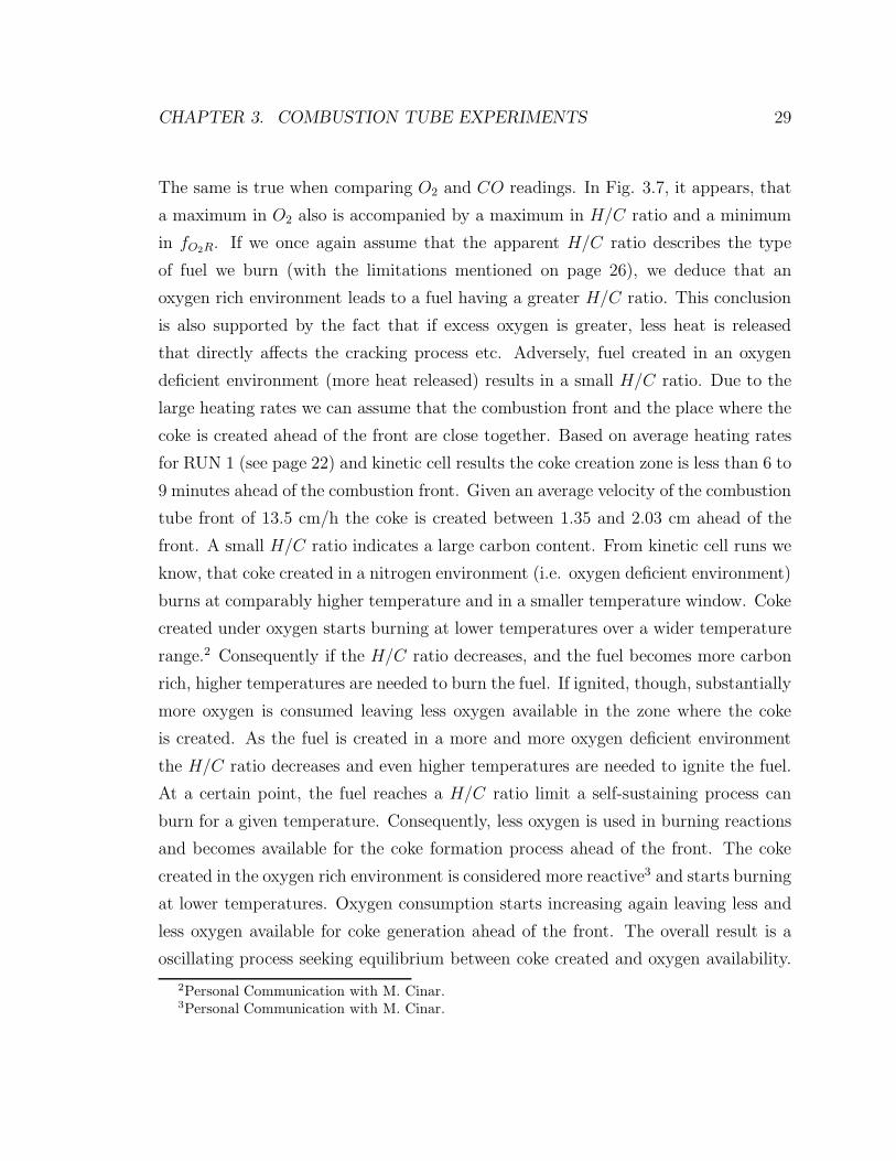
The same is true when comparing O2 and CO readings. In Fig. 3.7, it appears, that
a maximum in O2 also is accompanied by a maximum in H/C ratio and a minimum
in fO2R. If we once again assume that the apparent H/C ratio describes the type
of fuel we burn (with the limitations mentioned on page 26), we deduce that an
oxygen rich environment leads to a fuel having a greater H/C ratio. This conclusion
is also supported by the fact that if excess oxygen is greater, less heat is released
that directly affects the cracking process etc. Adversely, fuel created in an oxygen
deficient environment (more heat released) results in a small H/C ratio. Due to the
large heating rates we can assume that the combustion front and the place where the
coke is created ahead of the front are close together. Based on average heating rates
for RUN 1 (see page 22) and kinetic cell results the coke creation zone is less than 6 to
9 minutes ahead of the combustion front. Given an average velocity of the combustion
tube front of 13.5 cm/h the coke is created between 1.35 and 2.03 cm ahead of the
front. A small H/C ratio indicates a large carbon content. From kinetic cell runs we
know, that coke created in a nitrogen environment (i.e. oxygen deficient environment)
burns at comparably higher temperature and in a smaller temperature window. Coke
created under oxygen starts burning at lower temperatures over a wider temperature
range.2 Consequently if the H/C ratio decreases, and the fuel becomes more carbon
rich, higher temperatures are needed to burn the fuel. If ignited, though, substantially
more oxygen is consumed leaving less oxygen available in the zone where the coke
is created. As the fuel is created in a more and more oxygen deficient environment
the H/C ratio decreases and even higher temperatures are needed to ignite the fuel.
At a certain point, the fuel reaches a H/C ratio limit a self-sustaining process can
burn for a given temperature. Consequently, less oxygen is used in burning reactions
and becomes available for the coke formation process ahead of the front. The coke
created in the oxygen rich environment is considered more reactive3 and starts burning
at lower temperatures. Oxygen consumption starts increasing again leaving less and
less oxygen available for coke generation ahead of the front. The overall result is a
oscillating process seeking equilibrium between coke created and oxygen availability.
2Personal Communication with M. Cinar.3Personal Communication with M. Cinar.
CHAPTER 3. COMBUSTION TUBE EXPERIMENTS 30
Therefore, when oxygen flow rate is just enough to sustain the front, and coke is
always created in an oxygen deficient environment, oscillations should disappear.
This behavior was observed for RUN 7 (see Fig. 3.22). In addition, for RUN 7 the
pressure was not adjusted. From the sampling process it is known that a change
in pressure also affects gas concentrations. An additional effect of pressure changes
cannot be ruled out.
3.5 Operational Data
Calculating operational data as summarized in Table A.15, the entire tube run was
taken into account. Values represent only rough estimates and are based on the
assumption that inlet and outlet flow rate are the same. Oil recovery is based on the
volume swept which is basically comprised of Burned Zone 1 and Burned Zone 2.
3.6 Repeatability
If we use stoichiometry as calculated previously, we obtain a certain value for CO2 and
CO for a given value of O2. In a simulation we will not be able to achieve completely
the same results because we cannot model preparation of the mixture, the packing
process etc. We should be, however, able to obtain the the same CO2 and CO values
for a given value of O2. Plotting the CO2 and CO versus O2 gives an idea, of the
range of values. The range will be a function of mixture, packing, stoichiometry, and
operating conditions. This helps to verify the simulation model. Furthermore, it is a
simple yet helpful consistency check.
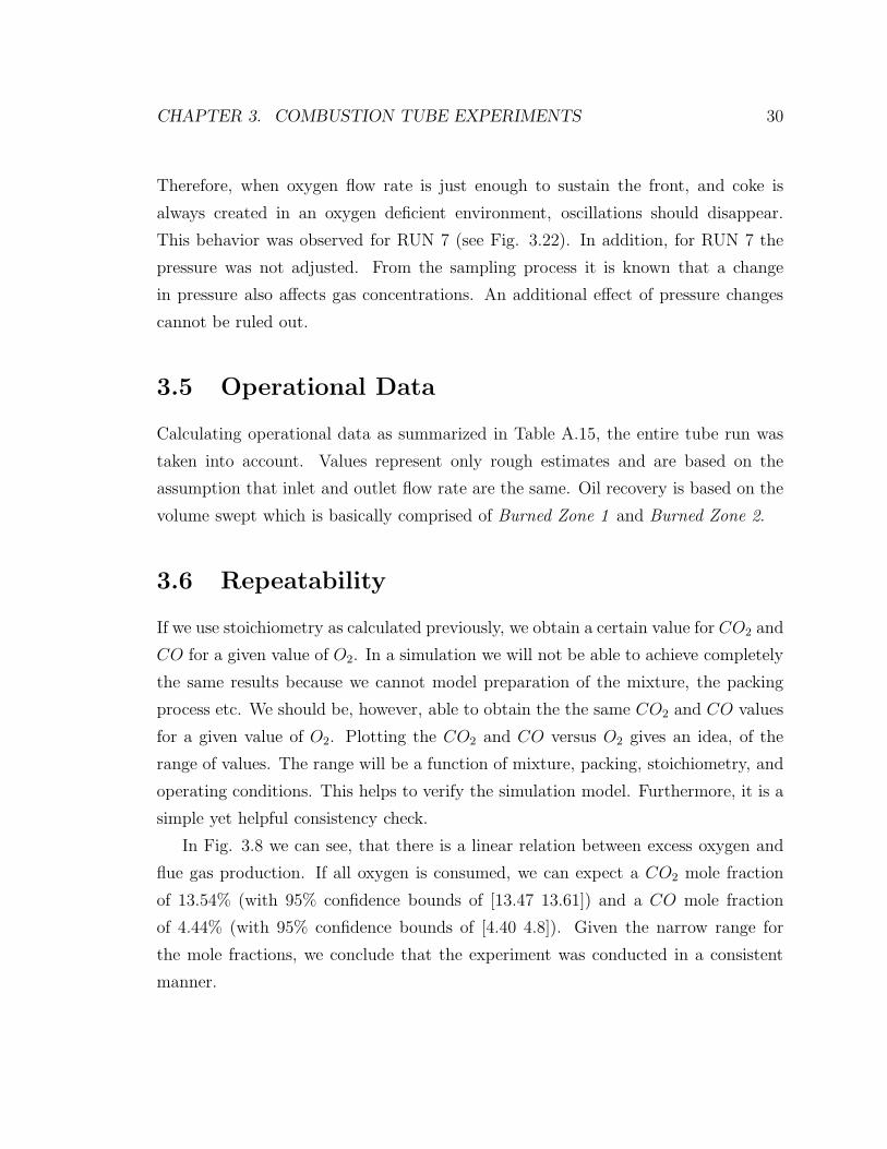
In Fig. 3.8 we can see, that there is a linear relation between excess oxygen and
flue gas production. If all oxygen is consumed, we can expect a CO2 mole fraction
of 13.54% (with 95% confidence bounds of [13.47 13.61]) and a CO mole fraction
of 4.44% (with 95% confidence bounds of [4.40 4.8]). Given the narrow range for
the mole fractions, we conclude that the experiment was conducted in a consistent
manner.
CHAPTER 3. COMBUSTION TUBE EXPERIMENTS 31
bbbbbbbbbbbbbbbb b b b b b b b b b b b b b b b b b b b b b b b b b b b b b b b b b b b b b b b b b b b b b b b bbbbbbbbbbbbbbb b b b b b b b b b b b b b b b b b b b b bbbbbbbbbbbbb
bbbbbbbbbb b b b b b b b b b b b b b b b b b b b b b b b b b bbbbbbbbbbbbb
bbbbbbbbbbb
bbbbbbbbbbb b b b b b b b b b b b bbbbbbbbbb b b b b b b b b b b b b b b b b b b b b b bbbbbbbbbbbbbbbbbbbbb
bbbbbbbbbbbbbbbbbbbbbbbb b b b b b b b b b b b b b b b b b b b b b b b b bbbbbb
bbbbbbbbbbbbbbbbbbbbbbbbbbbbbbbbbbbbbb
bbbbbb bb b b b b b b b b b b b b b b b b b b b b b b b b b b b b bbbbbbb b b b b b b b b b b b b b b b b b b b b b b bbbbbbbb
bbbbbbbbbbbbb
bbbbbbbb
bbbbbbbbbbb b b b bb b b b b b b b b b b b b b b b b b b b b b b b b b b b b b b b b b b b b b b b b b b bbbbbbbb
bbbbbbb
bbbbbbbbb
bbbbbbbbbbbbbbb b b b b bbbbbb
bbbbbb
bbbbbbbbbb b b b b b b b b b b b b b b b b b b b b b b b b b b b bbbbbbbb
bbbbbbbbbbbbb
bbbbbb
bbbbbbb b b b b b b b b b b b b b b b b b b b b b b b b b b b b b b b b b b b
bbbbbbbbbbbbbbbb b b b b b b b b b b b b b b b b b b b b b b b b b b b b b b b b b b b b b b b b b b b b b b b bbbbbbbbbbbbbbb b b b b b b b b b b b b b b b b b b b b bbbbbbbbbbbbbbbbbbbbbbb b b b b b b b b b b b b b b b b b b b b b b b b b bbbbbbbbbbbbbbbbbbbbbbbbbbbbbb
bbbbb b b b b b b b b b b b bbbbbbbbbb b b b b b b b b b b b b b b b b b b b b b bbbbbbbbbbbbbbbbbbbbbbbbbbbbbbbbbbbbbbbbbbbbb b b b b b b b b b b b b b b b b b b b b b b b b bbbbbbbbbbbbbbbbbbbbbbbbbbbbbbbbbbbbbbbbb
bbbbbbbbb b b b b b b b b b b b b b b b b b b b b b b b b b b b b b b bbbbbbb b b b b b b b b b b b b b b b b b b b b b b bbbbbbbbbbbbbbbbbbbbbbbbbbbbbbbbbbbbbbbb b b b bb b b b b b b b b b b b b b b b b b b b b b b b b b b b b b b b b b b b b b b b b b b bbbbbbbbbbbbbbb
bbbbbbbbbbbbbbbbbbbbbbbb b b b b bbbbbbbbbbbbbbbbbb
bbbb b b b b b b b b b b b b b b b b b b b b b b b b b b b bbbbbbbbbbbbbbbbbbbbbbbbbbbbbbbbbb b b b b b b b b b b b b b b b b b b b b b b b b b b b b b b b b b b b
0
1
2
3
4
5
6
7
8
9
10
11
12
13
14
15
16
0 1 2 3 4 5 6 7 8 9 10 110
1
2
3
4
5
6
7
8
9
10
11
12
13
14
15
16M
olarFra
ction
CO
2and
CO
(-) M
olarFra
ctio
nCO
2and
CO
(-)
Molar Fraction O2 (-)
CO2 vs. O2
CO vs. O2
CO2 = −p1 × O2 + p2
Coefficients (with 95% confidence bounds):
p1=-0.6953 (-0.7092, -0.6814)
p2=13.54 (13.47, 13.61)
CO = −p1 × O2 + p2
Coefficients (with 95% confidence bounds):
p1=-0.2208 (-0.2286, -0.2129)
p1=4.44 (4.401, 4.479)
Figure 3.8: CO2 and CO as a function of excess O2 for RUN 1.
3.7 Individual Combustion Tube Results
3.7.1 RUN 1
All experimental results for RUN 1 were used to describe the post-processing steps
above. Gas phase parameters and operational data is summarized in Table A.16 and
Table A.15 respectively. Production data is given in Table A.7.
3.7.2 RUN 2
RUN 2 served as a control experiment for RUN 1. Basically the same experimental
setup was used (see Table A.6 for sample mixtures). Again air flow rate was 3 l/min
and pressure was held constant at 100 psi. For the stabilized zone a velocity of 13.9
cm/h is obtained.4
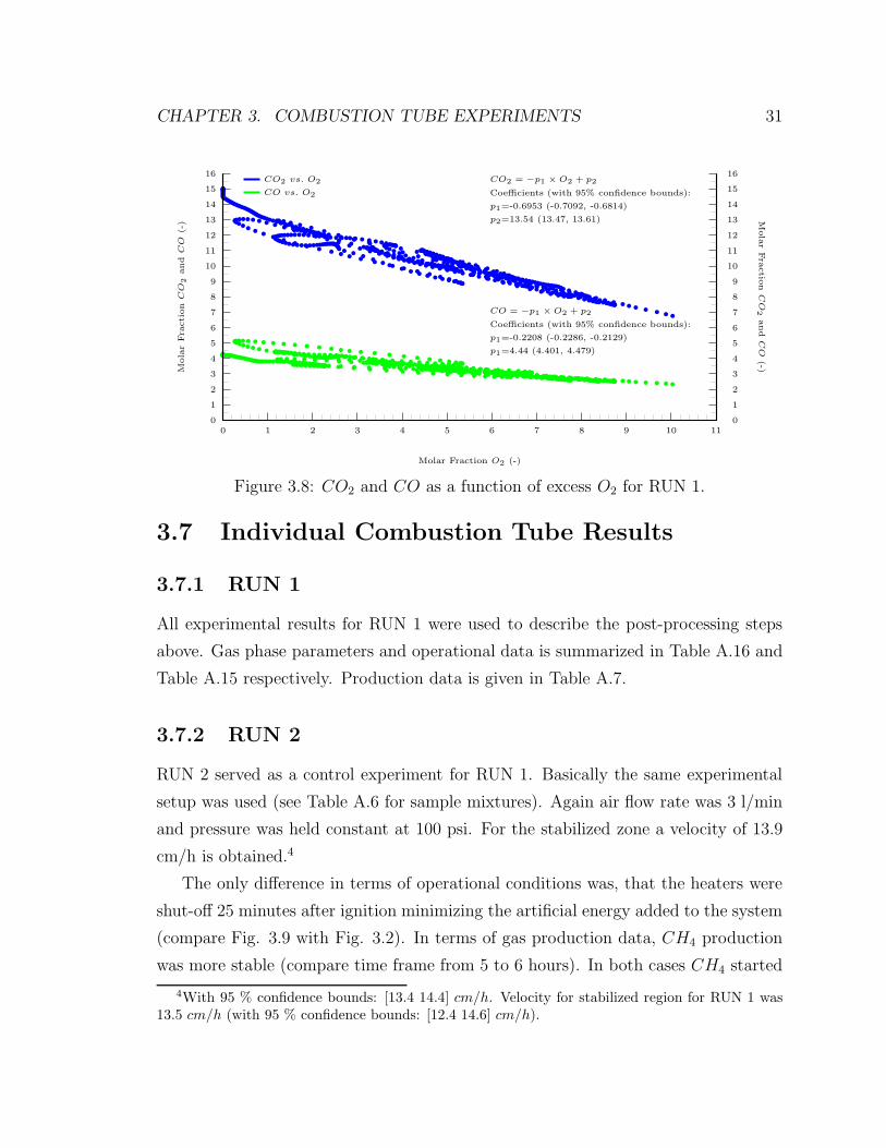
The only difference in terms of operational conditions was, that the heaters were
shut-off 25 minutes after ignition minimizing the artificial energy added to the system
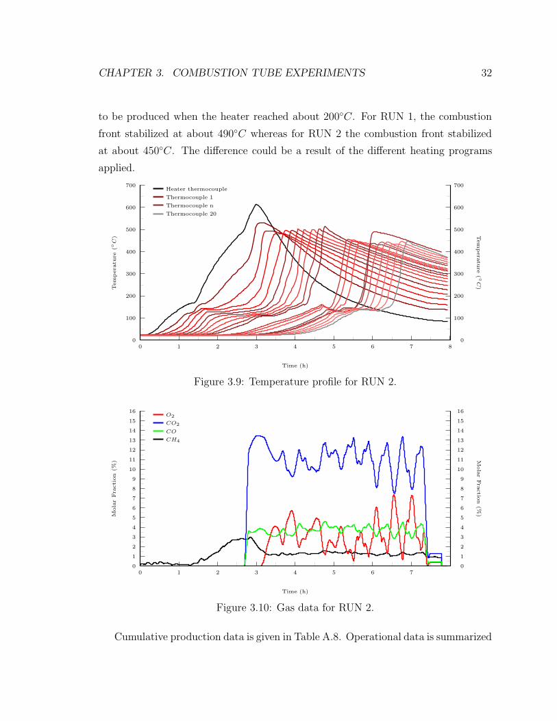
(compare Fig. 3.9 with Fig. 3.2). In terms of gas production data, CH4 production
was more stable (compare time frame from 5 to 6 hours). In both cases CH4 started
4With 95 % confidence bounds: [13.4 14.4] cm/h. Velocity for stabilized region for RUN 1 was13.5 cm/h (with 95 % confidence bounds: [12.4 14.6] cm/h).
CHAPTER 3. COMBUSTION TUBE EXPERIMENTS 32
to be produced when the heater reached about 200◦C. For RUN 1, the combustion
front stabilized at about 490◦C whereas for RUN 2 the combustion front stabilized
at about 450◦C. The difference could be a result of the different heating programs
applied.
0
100
200
300
400
500
600
700
0 1 2 3 4 5 6 7 80
100
200
300
400
500
600
700
Tem
pera
ture
(◦C) T
em
pera
ture
(◦C)
Time (h)
Heater thermocouple
Thermocouple 1
Thermocouple n
Thermocouple 20
Figure 3.9: Temperature profile for RUN 2.
0
1
2
3
4
5
6
7
8
9
10
11
12
13
14
15
16
0 1 2 3 4 5 6 70
1
2
3
4
5
6
7
8
9
10
11
12
13
14
15
16
MolarFra
ction
(%) M
olarFra
ctio
n(%
)
Time (h)
O2
CO2
CO
CH4
Figure 3.10: Gas data for RUN 2.
Cumulative production data is given in Table A.8. Operational data is summarized
CHAPTER 3. COMBUSTION TUBE EXPERIMENTS 33
in Table A.15. The overall H/C Ratio is the same compared to RUN 1. In RUN
2, though, more fuel was consumed (23.2 kg/m3 versus 18.8 kg/m3) resulting in
comparably higher air requirements (291 m3(ST )/m3 versus 248 m3(ST )/m3).
The result of the post mortem analysis is summarized in Table A.17. For RUN 2
almost twice the amount of pyrolysis coke was obtained. This is understandable be-
cause heaters were turned off considerably earlier compared to RUN 1. Less artificial
heat was, therefore, available to burn this type of coke. In terms of stoichiometry
for the stabilized region, however, both runs are the same (compare Eq. 3.5 with
Eq. 3.4).5 In either case the same fuel is burned and both runs suggest that HTO
reactions dominate.
CH1.26 + 1.41O2 + 5.41N2 −→
0.74CO2 + 0.26CO + 0.23O2 + 0.63H2O + 5.41N2 (3.5)
The same is true to a great extent for gas phase parameters (see Table A.16). Fig.
3.11 shows selected parameters for the entire experiment (compare with Fig. 3.8). In
the oxygen consumption curve we can see artifacts from the sampling spike removal
process (e.g. 6.8 hours into the experiment, positive flank of the oxygen consumption
curve). As mentioned above, during each sampling process the tube is shut-in for half
a minute and then opened again. This causes air to flush through the tube and fill
the previously emptied sample bomb volume. The air flush causes the combustion
front to increase in temperature momentarily and the coke created ahead will be less
hydrogen rich. As a result we can see a subsequent drop in H/C ratio. Once the
lower H/C ratio fuel is burned, the previous trend continues.
5We have to keep in mind that calculating operational data is subject to personal interpretatione.g. defining zones during the post mortem. Comparing stoichiometry is more objective.
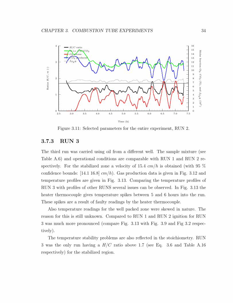
CHAPTER 3. COMBUSTION TUBE EXPERIMENTS 34
0
1
2
3
4
2.5 3.0 3.5 4.0 4.5 5.0 5.5 6.0 6.5 7.0 7.50
1
2
3
4
5
6
7
8
9
10
11
12
13
14
15
16RatiosH
/C,m
(-)
Molarfra
ctio
nO
2,CO
2(%
),and
fO
2R
(101)
Time (h)
H/C ratio
m i.e. CO/CO2
O2 excess
CO2 produced
fO2R
Figure 3.11: Selected parameters for the entire experiment, RUN 2.
3.7.3 RUN 3
The third run was carried using oil from a different well. The sample mixture (see
Table A.6) and operational conditions are comparable with RUN 1 and RUN 2 re-
spectively. For the stabilized zone a velocity of 15.4 cm/h is obtained (with 95 %
confidence bounds: [14.1 16.8] cm/h). Gas production data is given in Fig. 3.12 and
temperature profiles are given in Fig. 3.13. Comparing the temperature profiles of
RUN 3 with profiles of other RUNS several issues can be observed. In Fig. 3.13 the
heater thermocouple gives temperature spikes between 5 and 6 hours into the run.
These spikes are a result of faulty readings by the heater thermocouple.
Also temperature readings for the well packed zone were skewed in nature. The
reason for this is still unknown. Compared to RUN 1 and RUN 2 ignition for RUN
3 was much more pronounced (compare Fig. 3.13 with Fig. 3.9 and Fig 3.2 respec-
tively).
The temperature stability problems are also reflected in the stoichiometry. RUN
3 was the only run having a H/C ratio above 1.7 (see Eq. 3.6 and Table A.16
respectively) for the stabilized region.
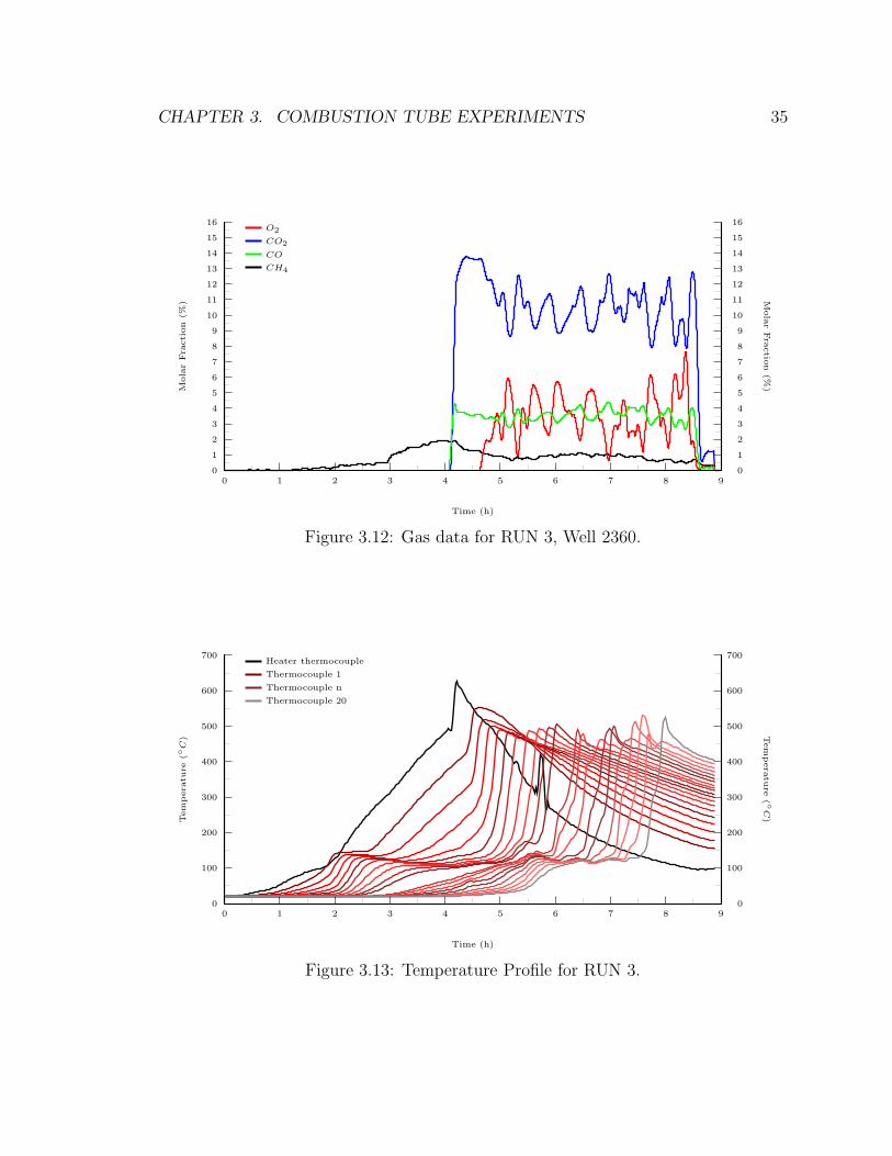
CHAPTER 3. COMBUSTION TUBE EXPERIMENTS 35
0
1
2
3
4
5
6
7
8
9
10
11
12
13
14
15
16
0 1 2 3 4 5 6 7 8 90
1
2
3
4
5
6
7
8
9
10
11
12
13
14
15
16
MolarFra
ction
(%) M
olarFra
ctio
n(%
)
Time (h)
O2
CO2
CO
CH4
Figure 3.12: Gas data for RUN 3, Well 2360.
0
100
200
300
400
500
600
700
0 1 2 3 4 5 6 7 8 90
100
200
300
400
500
600
700
Tem
pera
ture
(◦C) T
em
pera
ture
(◦C)
Time (h)
Heater thermocouple
Thermocouple 1
Thermocouple n
Thermocouple 20
Figure 3.13: Temperature Profile for RUN 3.

CHAPTER 3. COMBUSTION TUBE EXPERIMENTS 36
CH1.86 + 2.65O2 + 5.97N2 −→
0.75CO2 + 0.25CO + 0.25O2 + 0.93H2O + 5.97N2 (3.6)
Considering the entire run, however, H/C ratio was at 1.45 (see Table A.15).
3.7.4 RUN 4
RUN 4 served as a control experiment for RUN 3. The same experimental setup was
used (see Table A.6 for the sample mixture). Again air flow rate was 3 l/min and
pressure was held constant at 100 psi. For the stabilized zone, a velocity of 15.4
cm/h is obtained (with 95 % confidence bounds: [14.2 16.6] cm/h). Gas production
data (see Fig. 3.14) is basically the same as for RUN 3 (see Fig. 3.12). For RUN
4 stabilization could be reached very early. Partial destabilization in gas production
data resulted from sampling. Also temperature profiles are the same. Again, when
the combustion front hit the well packed zone initial temperature profiles got skewed
(see Fig. 3.15). In terms products, stoichiometry of RUN 4 (see Eq. 3.7) and RUN 3
(see Eq. 3.6) give comparable results. Concerning reactants RUN 4 has a significant
lower H/C ratio (see Table A.16).
CH1.37 + 1.41O2 + 5.42N2 −→
0.74CO2 + 0.26CO + 0.20O2 + 0.69H2O + 5.42N2 (3.7)
The fact, that the same experimental conditions can yield different H/C ratios
point out the importance of control experiments. In terms of operational data (see
Table A.15) the second highest oil recovery was obtained.
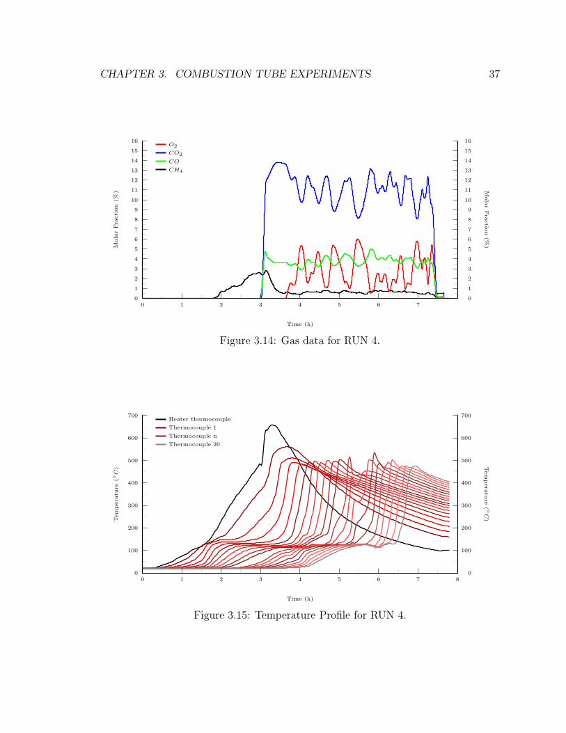
CHAPTER 3. COMBUSTION TUBE EXPERIMENTS 37
0
1
2
3
4
5
6
7
8
9
10
11
12
13
14
15
16
0 1 2 3 4 5 6 70
1
2
3
4
5
6
7
8
9
10
11
12
13
14
15
16
MolarFra
ction
(%) M
olarFra
ctio
n(%
)
Time (h)
O2
CO2
CO
CH4
Figure 3.14: Gas data for RUN 4.
0
100
200
300
400
500
600
700
0 1 2 3 4 5 6 7 80
100
200
300
400
500
600
700
Tem
pera
ture
(◦C) T
em
pera
ture
(◦C)
Time (h)
Heater thermocouple
Thermocouple 1
Thermocouple n
Thermocouple 20
Figure 3.15: Temperature Profile for RUN 4.
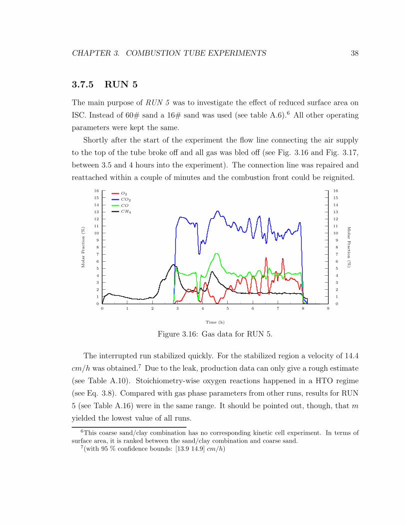
CHAPTER 3. COMBUSTION TUBE EXPERIMENTS 38
3.7.5 RUN 5
The main purpose of RUN 5 was to investigate the effect of reduced surface area on
ISC. Instead of 60# sand a 16# sand was used (see table A.6).6 All other operating
parameters were kept the same.
Shortly after the start of the experiment the flow line connecting the air supply
to the top of the tube broke off and all gas was bled off (see Fig. 3.16 and Fig. 3.17,
between 3.5 and 4 hours into the experiment). The connection line was repaired and
reattached within a couple of minutes and the combustion front could be reignited.
0
1
2
3
4
5
6
7
8
9
10
11
12
13
14
15
16
0 1 2 3 4 5 6 7 8 90
1
2
3
4
5
6
7
8
9
10
11
12
13
14
15
16
MolarFra
ction
(%) M
olarFra
ctio
n(%
)
Time (h)
O2
CO2
CO
CH4
Figure 3.16: Gas data for RUN 5.
The interrupted run stabilized quickly. For the stabilized region a velocity of 14.4
cm/h was obtained.7 Due to the leak, production data can only give a rough estimate
(see Table A.10). Stoichiometry-wise oxygen reactions happened in a HTO regime
(see Eq. 3.8). Compared with gas phase parameters from other runs, results for RUN
5 (see Table A.16) were in the same range. It should be pointed out, though, that m
yielded the lowest value of all runs.
6This coarse sand/clay combination has no corresponding kinetic cell experiment. In terms ofsurface area, it is ranked between the sand/clay combination and coarse sand.
7(with 95 % confidence bounds: [13.9 14.9] cm/h)
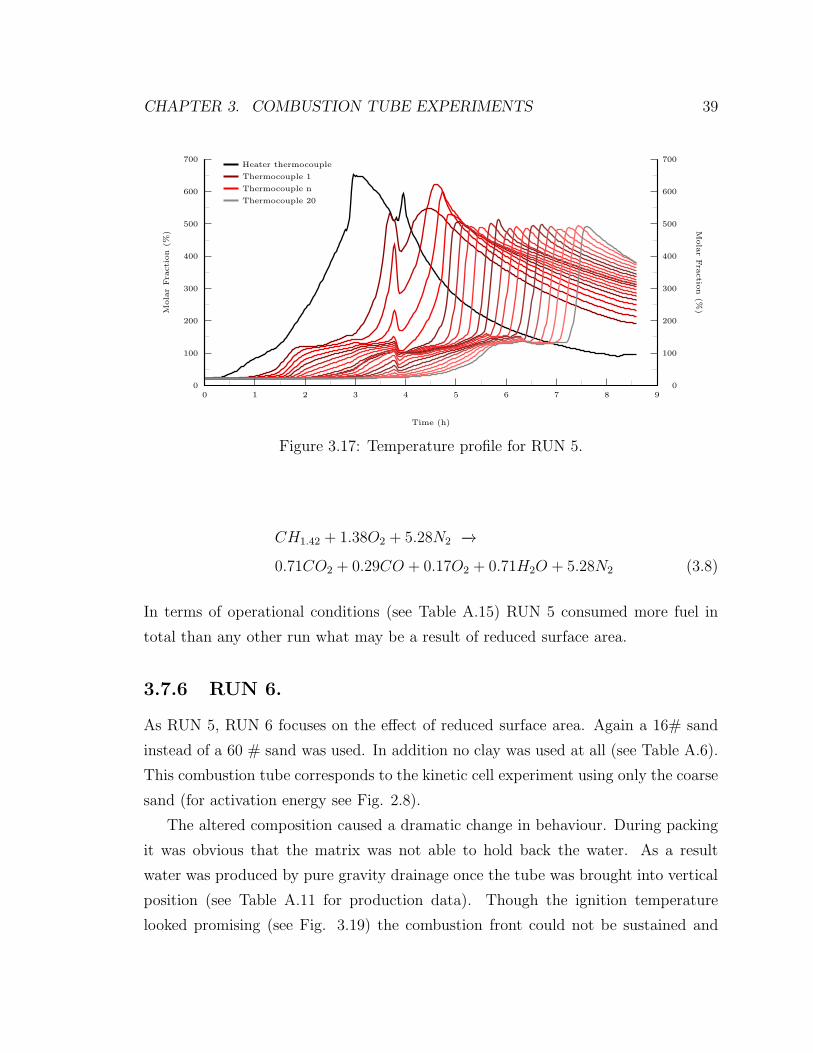
CHAPTER 3. COMBUSTION TUBE EXPERIMENTS 39
0
100
200
300
400
500
600
700
0 1 2 3 4 5 6 7 8 90
100
200
300
400
500
600
700M
olarFra
ction
(%) M
olarFra
ctio
n(%
)
Time (h)
Heater thermocouple
Thermocouple 1
Thermocouple n
Thermocouple 20
Figure 3.17: Temperature profile for RUN 5.
CH1.42 + 1.38O2 + 5.28N2 −→
0.71CO2 + 0.29CO + 0.17O2 + 0.71H2O + 5.28N2 (3.8)
In terms of operational conditions (see Table A.15) RUN 5 consumed more fuel in
total than any other run what may be a result of reduced surface area.
3.7.6 RUN 6.
As RUN 5, RUN 6 focuses on the effect of reduced surface area. Again a 16# sand
instead of a 60 # sand was used. In addition no clay was used at all (see Table A.6).
This combustion tube corresponds to the kinetic cell experiment using only the coarse
sand (for activation energy see Fig. 2.8).
The altered composition caused a dramatic change in behaviour. During packing
it was obvious that the matrix was not able to hold back the water. As a result
water was produced by pure gravity drainage once the tube was brought into vertical
position (see Table A.11 for production data). Though the ignition temperature
looked promising (see Fig. 3.19) the combustion front could not be sustained and
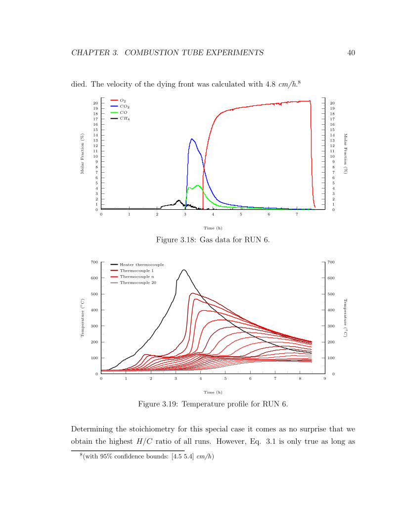
CHAPTER 3. COMBUSTION TUBE EXPERIMENTS 40
died. The velocity of the dying front was calculated with 4.8 cm/h.8
0
1
2
3
4
5
6
7
8
9
10
11
12
13
14
15
16
17
18
19
20
0 1 2 3 4 5 6 70
1
2
3
4
5
6
7
8
9
10
11
12
13
14
15
16
17
18
19
20
MolarFra
ction
(%) M
olarFra
ctio
n(%
)
Time (h)
O2
CO2
CO
CH4
Figure 3.18: Gas data for RUN 6.
0
100
200
300
400
500
600
700
0 1 2 3 4 5 6 7 8 90
100
200
300
400
500
600
700
Tem
pera
ture
(◦C) T
em
pera
ture
(◦C)
Time (h)
Heater thermocouple
Thermocouple 1
Thermocouple n
Thermocouple 20
Figure 3.19: Temperature profile for RUN 6.
Determining the stoichiometry for this special case it comes as no surprise that we
obtain the highest H/C ratio of all runs. However, Eq. 3.1 is only true as long as
8(with 95% confidence bounds: [4.5 5.4] cm/h)
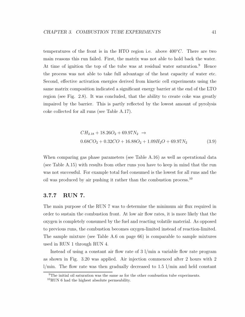
CHAPTER 3. COMBUSTION TUBE EXPERIMENTS 41
temperatures of the front is in the HTO region i.e. above 400◦C. There are two
main reasons this run failed. First, the matrix was not able to hold back the water.
At time of ignition the top of the tube was at residual water saturation.9 Hence
the process was not able to take full advantage of the heat capacity of water etc.
Second, effective activation energies derived from kinetic cell experiments using the
same matrix composition indicated a significant energy barrier at the end of the LTO
region (see Fig. 2.8). It was concluded, that the ability to create coke was greatly
impaired by the barrier. This is partly reflected by the lowest amount of pyrolysis
coke collected for all runs (see Table A.17).
CH2.18 + 18.26O2 + 69.97N2 −→
0.68CO2 + 0.32CO + 16.88O2 + 1.09H2O + 69.97N2 (3.9)
When comparing gas phase parameters (see Table A.16) as well as operational data
(see Table A.15) with results from other runs you have to keep in mind that the run
was not successful. For example total fuel consumed is the lowest for all runs and the
oil was produced by air pushing it rather than the combustion process.10
3.7.7 RUN 7.
The main purpose of the RUN 7 was to determine the minimum air flux required in
order to sustain the combustion front. At low air flow rates, it is more likely that the
oxygen is completely consumed by the fuel and reacting volatile material. As opposed
to previous runs, the combustion becomes oxygen-limited instead of reaction-limited.
The sample mixture (see Table A.6 on page 66) is comparable to sample mixtures
used in RUN 1 through RUN 4.
Instead of using a constant air flow rate of 3 l/min a variable flow rate program
as shown in Fig. 3.20 was applied. Air injection commenced after 2 hours with 2
l/min. The flow rate was then gradually decreased to 1.5 l/min and held constant
9The initial oil saturation was the same as for the other combustion tube experiments.10RUN 6 had the highest absolute permeability.
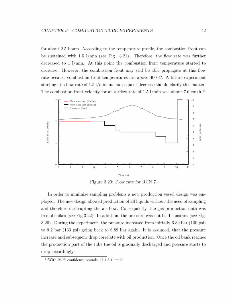
CHAPTER 3. COMBUSTION TUBE EXPERIMENTS 42
for about 2.5 hours. According to the temperature profile, the combustion front can
be sustained with 1.5 l/min (see Fig. 3.21). Therefore, the flow rate was further
decreased to 1 l/min. At this point the combustion front temperature started to
decrease. However, the combustion front may still be able propagate at this flow
rate because combustion front temperatures are above 400◦C. A future experiment
starting at a flow rate of 1.5 l/min and subsequent decrease should clarify this matter.
The combustion front velocity for an airflow rate of 1.5 l/min was about 7.6 cm/h.11
0
1
2
3
0 1 2 3 4 5 6 7 8 9 10 110
1
2
3
4
5
6
7
8
9
10
Flow
rate
(l/m
in) P
ressu
re(b
ar)
Time (h)
Flow rate N2 (l/min)
Flow rate Air (l/min)
Pressure (bar)
Figure 3.20: Flow rate for RUN 7.
In order to minimize sampling problems a new production vessel design was em-
ployed. The new design allowed production of all liquids without the need of sampling
and therefore interrupting the air flow. Consequently, the gas production data was
free of spikes (see Fig 3.22). In addition, the pressure was not held constant (see Fig.
3.20). During the experiment, the pressure increased from initially 6.89 bar (100 psi)
to 9.2 bar (133 psi) going back to 6.89 bar again. It is assumed, that the pressure
increase and subsequent drop correlate with oil production. Once the oil bank reaches
the production part of the tube the oil is gradually discharged and pressure starts to
drop accordingly.
11With 95 % confidence bounds: [7.1 8.1] cm/h.
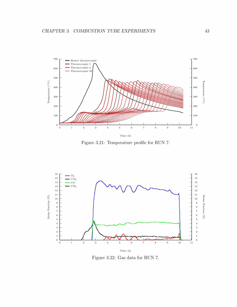
CHAPTER 3. COMBUSTION TUBE EXPERIMENTS 43
0
100
200
300
400
500
600
700
0 1 2 3 4 5 6 7 8 9 10 110
100
200
300
400
500
600
700
Tem
pera
ture
(◦C) T
em
pera
ture
(◦C)
Time (h)
Heater thermocouple
Thermocouple 1
Thermocouple n
Thermocouple 20
Figure 3.21: Temperature profile for RUN 7.
0
1
2
3
4
5
6
7
8
9
10
11
12
13
14
15
16
0 1 2 3 4 5 6 7 8 9 10 110
1
2
3
4
5
6
7
8
9
10
11
12
13
14
15
16
MolarFra
ction
(%) M
olarFra
ctio
n(%
)
Time (h)
O2
CO2
CO
CH4
Figure 3.22: Gas data for RUN 7.
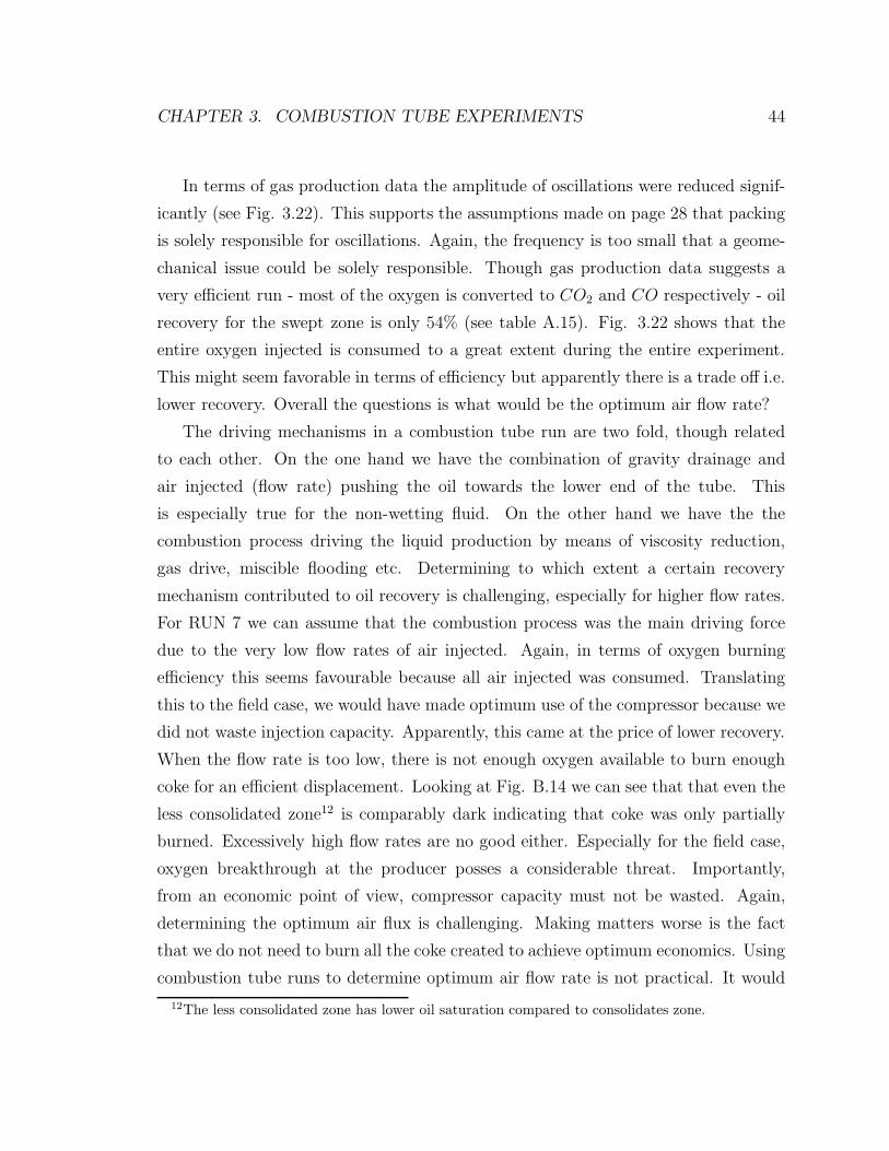
CHAPTER 3. COMBUSTION TUBE EXPERIMENTS 44
In terms of gas production data the amplitude of oscillations were reduced signif-
icantly (see Fig. 3.22). This supports the assumptions made on page 28 that packing
is solely responsible for oscillations. Again, the frequency is too small that a geome-
chanical issue could be solely responsible. Though gas production data suggests a
very efficient run - most of the oxygen is converted to CO2 and CO respectively - oil
recovery for the swept zone is only 54% (see table A.15). Fig. 3.22 shows that the
entire oxygen injected is consumed to a great extent during the entire experiment.
This might seem favorable in terms of efficiency but apparently there is a trade off i.e.
lower recovery. Overall the questions is what would be the optimum air flow rate?
The driving mechanisms in a combustion tube run are two fold, though related
to each other. On the one hand we have the combination of gravity drainage and
air injected (flow rate) pushing the oil towards the lower end of the tube. This
is especially true for the non-wetting fluid. On the other hand we have the the
combustion process driving the liquid production by means of viscosity reduction,
gas drive, miscible flooding etc. Determining to which extent a certain recovery
mechanism contributed to oil recovery is challenging, especially for higher flow rates.
For RUN 7 we can assume that the combustion process was the main driving force
due to the very low flow rates of air injected. Again, in terms of oxygen burning
efficiency this seems favourable because all air injected was consumed. Translating
this to the field case, we would have made optimum use of the compressor because we
did not waste injection capacity. Apparently, this came at the price of lower recovery.
When the flow rate is too low, there is not enough oxygen available to burn enough
coke for an efficient displacement. Looking at Fig. B.14 we can see that that even the
less consolidated zone12 is comparably dark indicating that coke was only partially
burned. Excessively high flow rates are no good either. Especially for the field case,
oxygen breakthrough at the producer posses a considerable threat. Importantly,
from an economic point of view, compressor capacity must not be wasted. Again,
determining the optimum air flux is challenging. Making matters worse is the fact
that we do not need to burn all the coke created to achieve optimum economics. Using
combustion tube runs to determine optimum air flow rate is not practical. It would
12The less consolidated zone has lower oil saturation compared to consolidates zone.
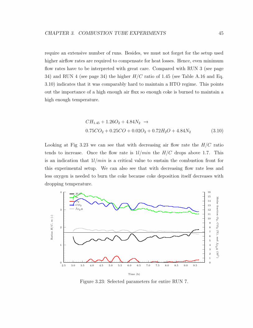
CHAPTER 3. COMBUSTION TUBE EXPERIMENTS 45
require an extensive number of runs. Besides, we must not forget for the setup used
higher airflow rates are required to compensate for heat losses. Hence, even minimum
flow rates have to be interpreted with great care. Compared with RUN 3 (see page
34) and RUN 4 (see page 34) the higher H/C ratio of 1.45 (see Table A.16 and Eq.
3.10) indicates that it was comparably hard to maintain a HTO regime. This points
out the importance of a high enough air flux so enough coke is burned to maintain a
high enough temperature.
CH1.45 + 1.26O2 + 4.84N2 −→
0.75CO2 + 0.25CO + 0.02O2 + 0.72H2O + 4.84N2 (3.10)
Looking at Fig 3.23 we can see that with decreasing air flow rate the H/C ratio
tends to increase. Once the flow rate is 1l/min the H/C drops above 1.7. This
is an indication that 1l/min is a critical value to sustain the combustion front for
this experimental setup. We can also see that with decreasing flow rate less and
less oxygen is needed to burn the coke because coke deposition itself decreases with
dropping temperature.
0
1
2
3
4
2.5 3.0 3.5 4.0 4.5 5.0 5.5 6.0 6.5 7.0 7.5 8.0 8.5 9.0 9.50
1
2
3
4
5
6
7
8
9
10
11
12
13
14
15
16
RatiosH
/C,m
(-)
Molarfra
ctio
nO
2,CO
2(%
),and
fO
2R
(101)
Time (h)
H/C
m
O2
CO2
fO2R
Figure 3.23: Selected parameters for entire RUN 7.
Chapter 4
Upscaling for In-Situ Combustion
Currently, most simulation studies related to in-situ combustion (ISC) are restricted
to modelling small laboratory scale problems such as kinetic cell and combustion tube
experiments. The transition from laboratory to field scale is still an unsolved problem
due to the very nature of the ISC process in combination with the discretization
techniques used to solve the convection-diffusion equations. In its simplest form we
use the following centered differencing scheme for approximation of a first derivative
transport term:
Ti+1 − Ti−1
2∆x=
∂T
∂x(xi) +
(∆x)2
6
∂3T
∂x3(ξ), xi−1 ≤ ξ ≤ xi+1 (4.1)
If T is sufficiently smooth, the scheme has O((∆x)2) accuracy. The scheme, however,
is well known to yield stability problems [31, 55]. Instead of the central difference
quotient a one-sided difference approximation in the direction of flow is preferably
used to foster stability. The scheme is given by
Ti − Ti−1
∆x=
∂T
∂x(xi)−
∆x
2
∂2T
∂x2(ξ), xi−1 ≤ ξ ≤ xi (4.2)
The accuracy for Eqn. 4.2 is only O(∆x) and we can show using a Taylor series that
46
CHAPTER 4. UPSCALING FOR IN-SITU COMBUSTION 47
Ti − Ti−1
∆x=
Ti+1 − Ti−1
2∆x−
∆x
2
(
Ti+1 − 2Ti + Ti−1
(∆x)2
)
=∂T
∂x(xi)−
∆x
2
∂2T
∂x2(xi) + O((∆x)2) (4.3)
Eqn. 4.3 is also referred to as upwind differencing and is essentially a O((∆x)2)
approximation to
∂T
∂x(xi)−
∆x
2
∂2T
∂x2(xi) (4.4)
instead of ∂T/∂x (xi). With ∂2T/∂x2 being a physical diffusion-like term this intro-
duced an artificial dispersion of size ∆x/2 [19]. Though artificial dispersion does help
to stabilize the difference method, the error induced in reservoir simulation is prob-
lematic. The magnitude of dispersion is directly proportional to the mesh spacing
∆x and is likely to smooth out sharp fronts. Fig. 4.1 illustrates what happens in the
case of loss of physics due to excessive smoothing and/or dispersion. Opposed to the
true temperature distribution in reservoir, cell block averaging and dispersion reduce
the maximum temperature below the reaction level prohibiting reactions from taking
place.
For ISC the chemical reaction front is physically very narrow and requires centimeter-
sized grids to be captured accurately. This is orders of magnitude smaller than af-
fordable grid block sizes for full field reservoir models. Accordingly, severe grid size
effects are encountered in full field-scale simulation making performance predictions
infeasible [17, 28]. In order to mitigate grid size effects both empirical [36] and spe-
cialized numerical techniques [26, 33], have been proposed with mixed results. None
of the techniques, however, made field-scale simulation practical in a commercial en-
vironment.
In 2011, Zhu et al. proposed a method based on a non-Arrhenius kinetic upscaling
approach similar to the classical analytical model of Gates and Ramey [25]. Instead of
resolving the combustion front on the grid, a subgrid-scale model is utilized capturing
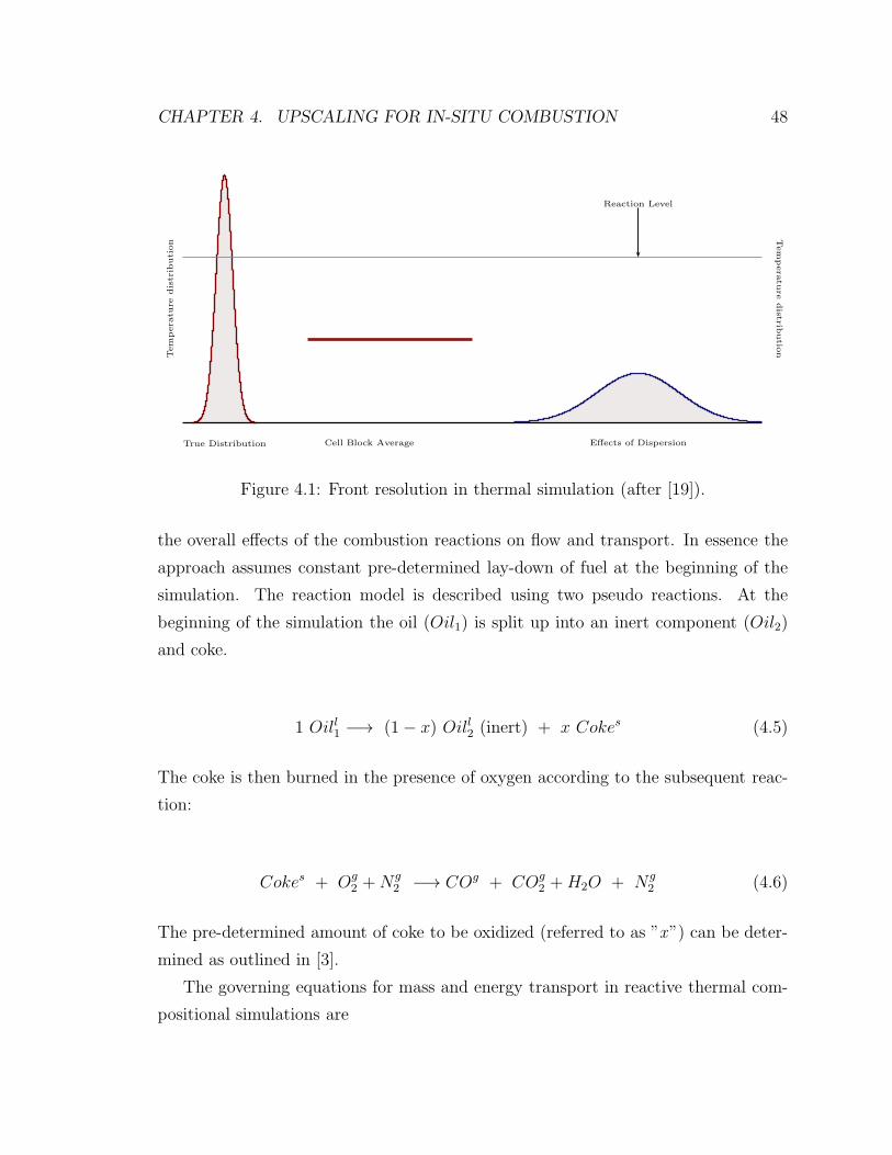
CHAPTER 4. UPSCALING FOR IN-SITU COMBUSTION 48
Tem
pera
ture
distrib
ution
Tem
pera
ture
distrib
utio
n
True Distribution Cell Block Average Effects of Dispersion
Reaction Level
Figure 4.1: Front resolution in thermal simulation (after [19]).
the overall effects of the combustion reactions on flow and transport. In essence the
approach assumes constant pre-determined lay-down of fuel at the beginning of the
simulation. The reaction model is described using two pseudo reactions. At the
beginning of the simulation the oil (Oil1) is split up into an inert component (Oil2)
and coke.
1 Oill1 −→ (1− x) Oill2 (inert) + x Cokes (4.5)
The coke is then burned in the presence of oxygen according to the subsequent reac-
tion:
Cokes + Og2 +Ng
2 −→ COg + COg2 +H2O + Ng
2 (4.6)
The pre-determined amount of coke to be oxidized (referred to as ”x”) can be deter-
mined as outlined in [3].
The governing equations for mass and energy transport in reactive thermal com-
positional simulations are
CHAPTER 4. UPSCALING FOR IN-SITU COMBUSTION 49
∂Ci
∂t+∇qi = Qwell
i +Qreaci (4.7)
∂Ut
∂t+∇
(
qh,adv + qh,cond)
= Qh,well +Qh,reac (4.8)
where Ci is the mass composition of i-th component, Ut is the total internal energy, qi
and qh,adv are advective mass and energy fluxes, Qwelli and Qh,well are the well terms,
and Qreaci and Qh,reac are the reaction terms.
Traditionally, Arrhenius kinetics are used for modelling ISC reactions. The reac-
tion rate for a grid cell is then given by
Qreaci = Vb × A× e
(
−Ea
R× T
)
×∏
j
(Cj)n (4.9)
where Vb is the rock bulk volume, A is the Arrhenius constant or pre-exponential
factor, Ea is the activation energy, R is the ideal gas constant, T is the local absolute
temperature, n is the reaction order, and Cj is the j-th reactant concentration. Cj is
defined as
Cj = Φ× bp × Sp × xj (4.10)
where p depicts the phase (oil, gas, or water), Φ is the porosity, S is the saturation,
b is the molar density, and x is the mole fraction.
The approach presented in [57] assumes an activation energy Ea of zero, reducing
Qreaci essentially to
Qreaci = Vb ×A×
∏
j
(Cj)n (4.11)
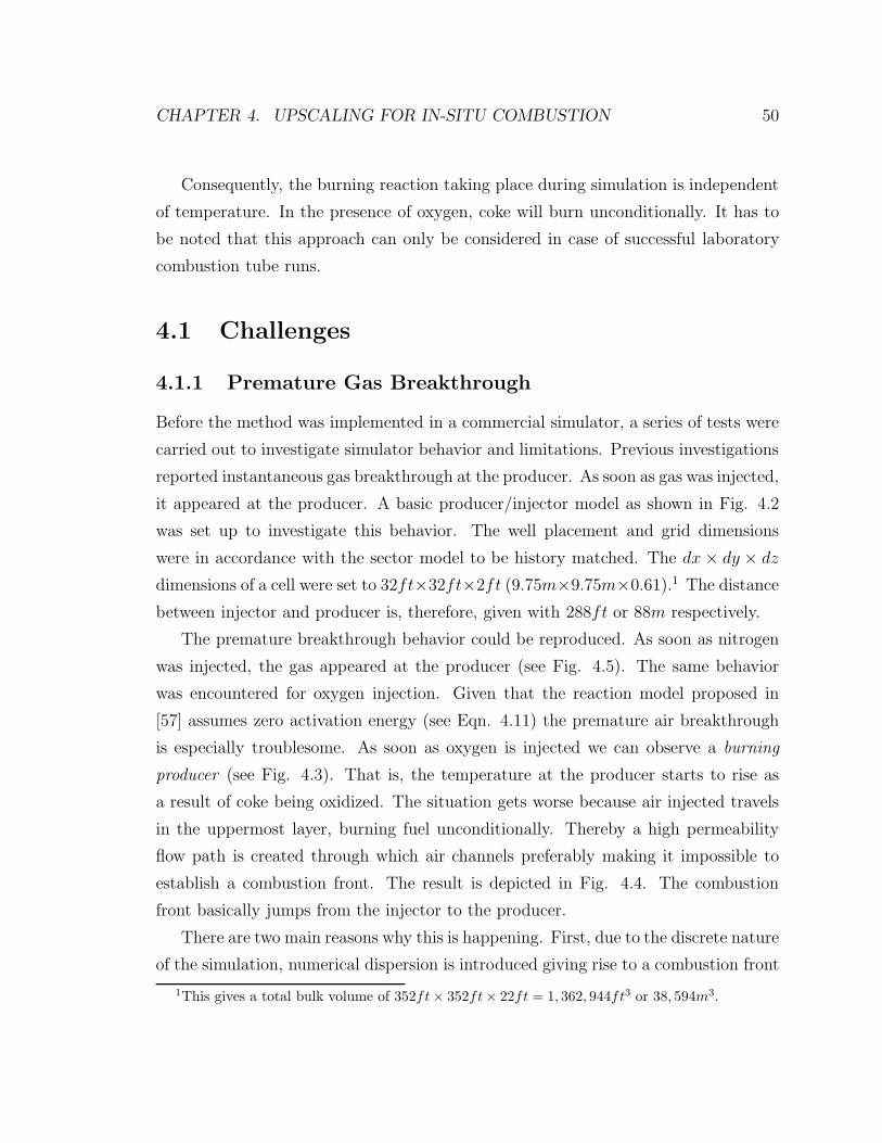
CHAPTER 4. UPSCALING FOR IN-SITU COMBUSTION 50
Consequently, the burning reaction taking place during simulation is independent
of temperature. In the presence of oxygen, coke will burn unconditionally. It has to
be noted that this approach can only be considered in case of successful laboratory
combustion tube runs.
4.1 Challenges
4.1.1 Premature Gas Breakthrough
Before the method was implemented in a commercial simulator, a series of tests were
carried out to investigate simulator behavior and limitations. Previous investigations
reported instantaneous gas breakthrough at the producer. As soon as gas was injected,
it appeared at the producer. A basic producer/injector model as shown in Fig. 4.2
was set up to investigate this behavior. The well placement and grid dimensions
were in accordance with the sector model to be history matched. The dx × dy × dz
dimensions of a cell were set to 32ft×32ft×2ft (9.75m×9.75m×0.61).1 The distance
between injector and producer is, therefore, given with 288ft or 88m respectively.
The premature breakthrough behavior could be reproduced. As soon as nitrogen
was injected, the gas appeared at the producer (see Fig. 4.5). The same behavior
was encountered for oxygen injection. Given that the reaction model proposed in
[57] assumes zero activation energy (see Eqn. 4.11) the premature air breakthrough
is especially troublesome. As soon as oxygen is injected we can observe a burning
producer (see Fig. 4.3). That is, the temperature at the producer starts to rise as
a result of coke being oxidized. The situation gets worse because air injected travels
in the uppermost layer, burning fuel unconditionally. Thereby a high permeability
flow path is created through which air channels preferably making it impossible to
establish a combustion front. The result is depicted in Fig. 4.4. The combustion
front basically jumps from the injector to the producer.
There are two main reasons why this is happening. First, due to the discrete nature
of the simulation, numerical dispersion is introduced giving rise to a combustion front
1This gives a total bulk volume of 352ft× 352ft× 22ft = 1, 362, 944ft3 or 38, 594m3.
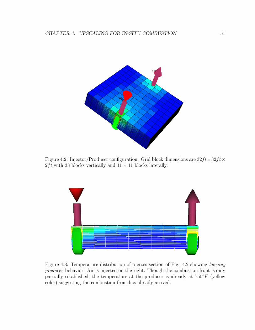
CHAPTER 4. UPSCALING FOR IN-SITU COMBUSTION 51
Figure 4.2: Injector/Producer configuration. Grid block dimensions are 32ft×32ft×2ft with 33 blocks vertically and 11× 11 blocks laterally.
Figure 4.3: Temperature distribution of a cross section of Fig. 4.2 showing burningproducer behavior. Air is injected on the right. Though the combustion front is onlypartially established, the temperature at the producer is already at 750◦F (yellowcolor) suggesting the combustion front has already arrived.
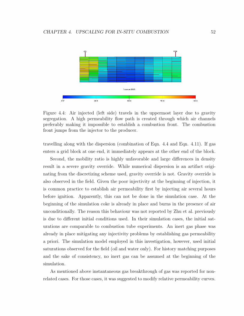
CHAPTER 4. UPSCALING FOR IN-SITU COMBUSTION 52
Figure 4.4: Air injected (left side) travels in the uppermost layer due to gravitysegregation. A high permeability flow path is created through which air channelspreferably making it impossible to establish a combustion front. The combustionfront jumps from the injector to the producer.
travelling along with the dispersion (combination of Eqn. 4.4 and Eqn. 4.11). If gas
enters a grid block at one end, it immediately appears at the other end of the block.
Second, the mobility ratio is highly unfavorable and large differences in density
result in a severe gravity override. While numerical dispersion is an artifact origi-
nating from the discretizing scheme used, gravity override is not. Gravity override is
also observed in the field. Given the poor injectivity at the beginning of injection, it
is common practice to establish air permeability first by injecting air several hours
before ignition. Apparently, this can not be done in the simulation case. At the
beginning of the simulation coke is already in place and burns in the presence of air
unconditionally. The reason this behaviour was not reported by Zhu et al. previously
is due to different initial conditions used. In their simulation cases, the initial sat-
urations are comparable to combustion tube experiments. An inert gas phase was
already in place mitigating any injectivity problems by establishing gas permeability
a priori. The simulation model employed in this investigation, however, used initial
saturations observed for the field (oil and water only). For history matching purposes
and the sake of consistency, no inert gas can be assumed at the beginning of the
simulation.
As mentioned above instantaneous gas breakthrough of gas was reported for non-
related cases. For those cases, it was suggested to modify relative permeability curves.
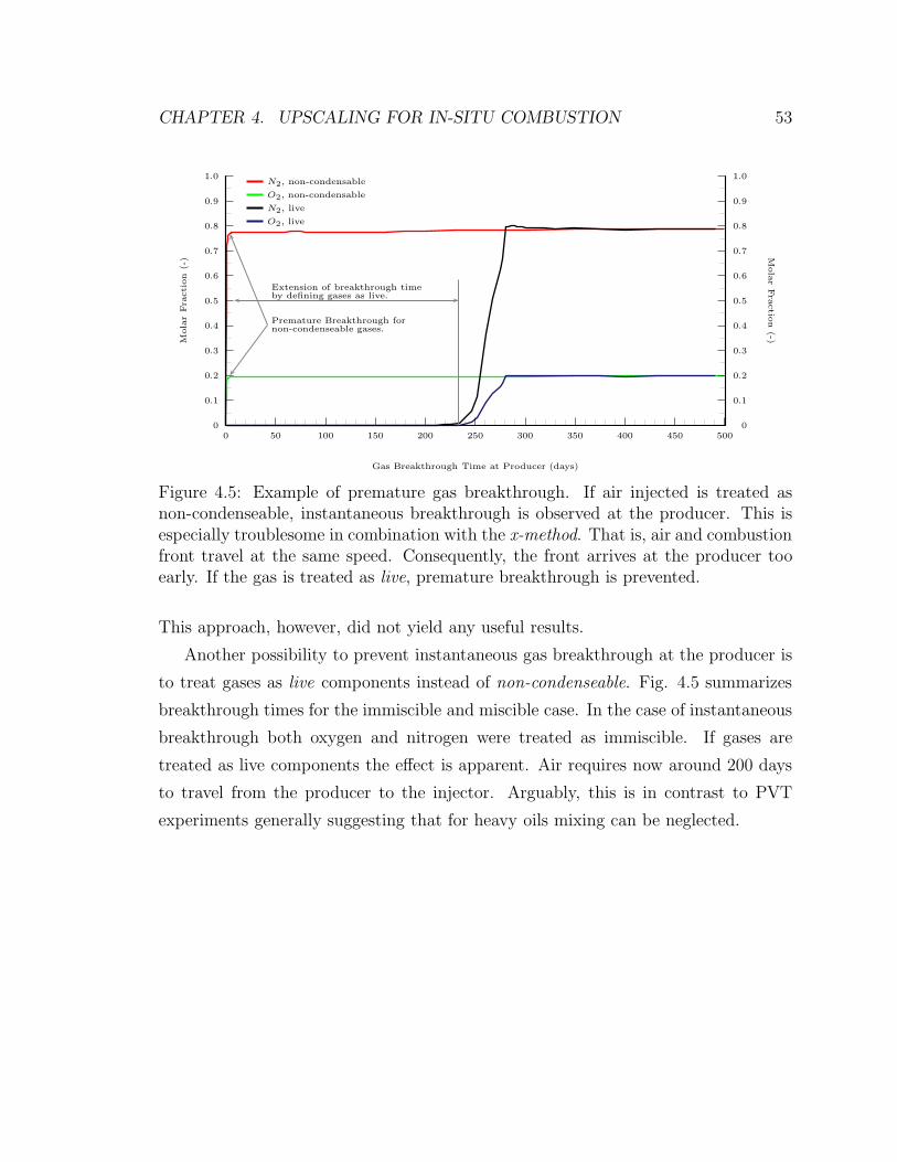
CHAPTER 4. UPSCALING FOR IN-SITU COMBUSTION 53
0
0.1
0.2
0.3
0.4
0.5
0.6
0.7
0.8
0.9
1.0
0 50 100 150 200 250 300 350 400 450 5000
0.1
0.2
0.3
0.4
0.5
0.6
0.7
0.8
0.9
1.0M
olarFra
ction
(-) M
olarFra
ctio
n(-)
Gas Breakthrough Time at Producer (days)
N2, non-condensable
O2, non-condensable
N2, live
O2, live
Extension of breakthrough timeby defining gases as live.
Premature Breakthrough fornon-condenseable gases.
Figure 4.5: Example of premature gas breakthrough. If air injected is treated asnon-condenseable, instantaneous breakthrough is observed at the producer. This isespecially troublesome in combination with the x-method. That is, air and combustionfront travel at the same speed. Consequently, the front arrives at the producer tooearly. If the gas is treated as live, premature breakthrough is prevented.
This approach, however, did not yield any useful results.
Another possibility to prevent instantaneous gas breakthrough at the producer is
to treat gases as live components instead of non-condenseable. Fig. 4.5 summarizes
breakthrough times for the immiscible and miscible case. In the case of instantaneous
breakthrough both oxygen and nitrogen were treated as immiscible. If gases are
treated as live components the effect is apparent. Air requires now around 200 days
to travel from the producer to the injector. Arguably, this is in contrast to PVT
experiments generally suggesting that for heavy oils mixing can be neglected.
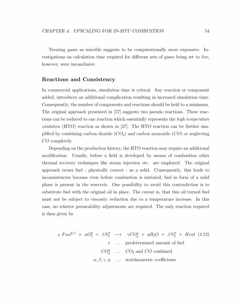
CHAPTER 4. UPSCALING FOR IN-SITU COMBUSTION 54
Treating gases as miscible suggests to be computationally more expensive. In-
vestigations on calculation time required for different sets of gases being set to live,
however, were inconclusive.
Reactions and Consistency
In commercial applications, simulation time is critical. Any reaction or component
added, introduces an additional complication resulting in increased simulation time.
Consequently, the number of components and reactions should be held to a minimum.
The original approach presented in [57] suggests two pseudo reactions. These reac-
tions can be reduced to one reaction which essentially represents the high temperature
oxidation (HTO) reaction as shown in [27]. The HTO reaction can be further sim-
plified by combining carbon dioxide (CO2) and carbon monoxide (CO) or neglecting
CO completely.
Depending on the production history, the HTO reaction may require an additional
modification. Usually, before a field is developed by means of combustion other
thermal recovery techniques like steam injection etc. are employed. The original
approach treats fuel - physically correct - as a solid. Consequently, this leads to
inconsistencies because even before combustion is initiated, fuel in form of a solid
phase is present in the reservoir. One possibility to avoid this contradiction is to
substitute fuel with the original oil in place. The caveat is, that this oil turned fuel
must not be subject to viscosity reduction due to a temperature increase. In this
case, no relative permeability adjustments are required. The only reaction required
is then given by
x Fuell/s + αOg2 + βNg
2 −→ γCOgy + ηH2O + βNg
2 + Heat (4.12)
x . . . predetermined amount of fuel
COgy . . . CO2 and CO combined
α, β, γ, η . . . stoichiometric coefficients
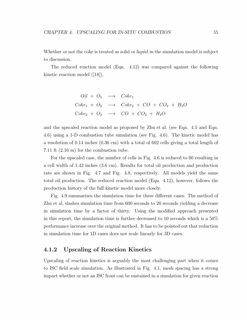
CHAPTER 4. UPSCALING FOR IN-SITU COMBUSTION 55
Whether or not the coke is treated as solid or liquid in the simulation model is subject
to discussion.
The reduced reaction model (Eqn. 4.12) was compared against the following
kinetic reaction model ([18]),
Oil + O2 −→ Coke1
Coke1 + O2 −→ Coke2 + CO + CO2 + H2O
Coke2 + O2 −→ CO + CO2 + H2O
and the upscaled reaction model as proposed by Zhu et al. (see Eqn. 4.5 and Eqn.
4.6) using a 1-D combustion tube simulation (see Fig. 4.6). The kinetic model has
a resolution of 0.14 inches (0.36 cm) with a total of 602 cells giving a total length of
7.11 ft (2.16 m) for the combustion tube.
For the upscaled case, the number of cells in Fig. 4.6 is reduced to 60 resulting in
a cell width of 1.42 inches (3.6 cm). Results for total oil production and production
rate are shown in Fig. 4.7 and Fig. 4.8, respectively. All models yield the same
total oil production. The reduced reaction model (Eqn. 4.12), however, follows the
production history of the full kinetic model more closely.
Fig. 4.9 summarizes the simulation time for three different cases. The method of
Zhu et al. slashes simulation time from 600 seconds to 20 seconds yielding a decrease
in simulation time by a factor of thirty. Using the modified approach presented
in this report, the simulation time is further decreased to 10 seconds which is a 50%
performance increase over the original method. It has to be pointed out that reduction
in simulation time for 1D cases does not scale linearly for 3D cases.
4.1.2 Upscaling of Reaction Kinetics
Upscaling of reaction kinetics is arguably the most challenging part when it comes
to ISC field scale simulation. As illustrated in Fig. 4.1, mesh spacing has a strong
impact whether or not an ISC front can be sustained in a simulation for given reaction
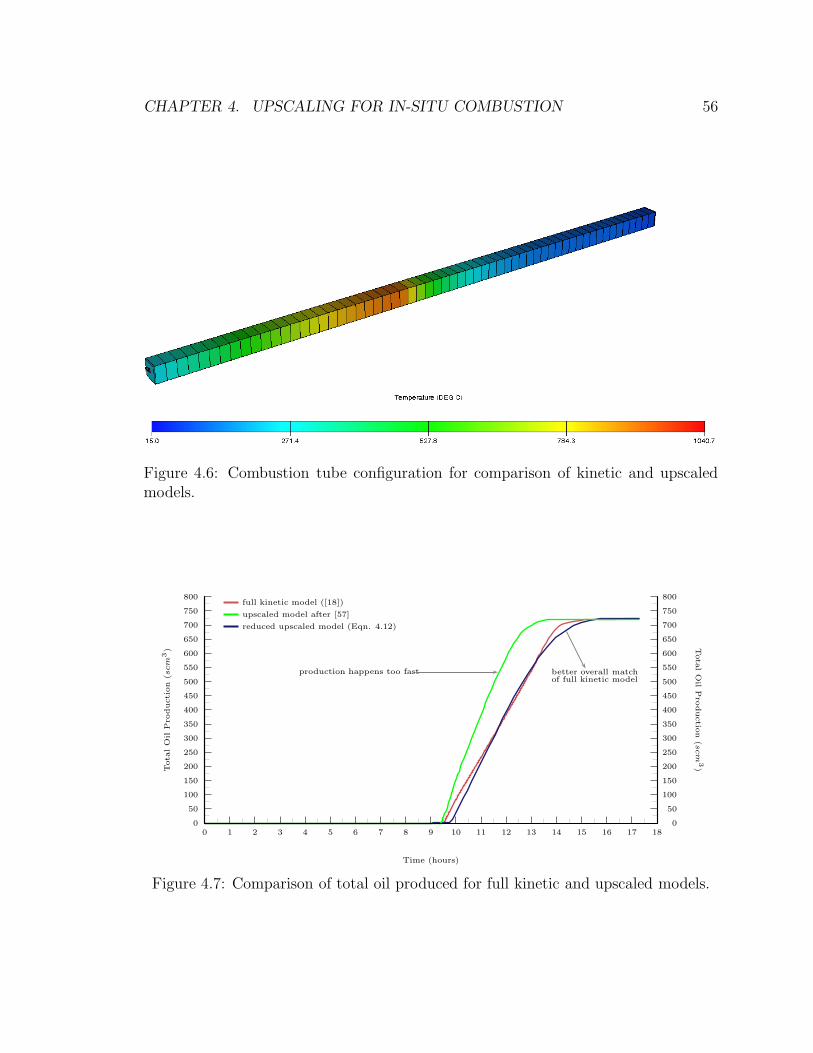
CHAPTER 4. UPSCALING FOR IN-SITU COMBUSTION 56
Figure 4.6: Combustion tube configuration for comparison of kinetic and upscaledmodels.
0
50
100
150
200
250
300
350
400
450
500
550
600
650
700
750
800
0 1 2 3 4 5 6 7 8 9 10 11 12 13 14 15 16 17 180
50
100
150
200
250
300
350
400
450
500
550
600
650
700
750
800
Tota
lOil
Pro
duction
(scm
3) T
ota
lOil
Pro
ductio
n(s
cm
3)
Time (hours)
full kinetic model ([18])
upscaled model after [57]
reduced upscaled model (Eqn. 4.12)
production happens too fast better overall matchof full kinetic model
Figure 4.7: Comparison of total oil produced for full kinetic and upscaled models.
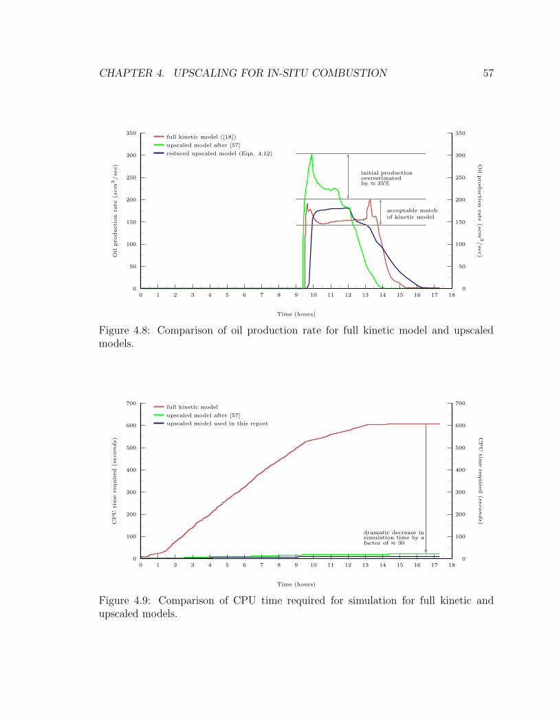
CHAPTER 4. UPSCALING FOR IN-SITU COMBUSTION 57
0
50
100
150
200
250
300
350
0 1 2 3 4 5 6 7 8 9 10 11 12 13 14 15 16 17 180
50
100
150
200
250
300
350
Oil
pro
duction
rate
(scm
3/sec) O
ilpro
ductio
nra
te(s
cm
3/sec)
Time (hours)
full kinetic model ([18])
upscaled model after [57]
reduced upscaled model (Eqn. 4.12)
initial productionoverestimatedby ≈ 35%
acceptable matchof kinetic model
Figure 4.8: Comparison of oil production rate for full kinetic model and upscaledmodels.
0
100
200
300
400
500
600
700
0 1 2 3 4 5 6 7 8 9 10 11 12 13 14 15 16 17 180
100
200
300
400
500
600
700
CPU
tim
ere
quired
(seconds) C
PU
timere
quire
d(s
econds)
Time (hours)
full kinetic model
upscaled model after [57]
upscaled model used in this report
dramatic decrease insimulation time by afactor of ≈ 30
Figure 4.9: Comparison of CPU time required for simulation for full kinetic andupscaled models.
CHAPTER 4. UPSCALING FOR IN-SITU COMBUSTION 58
set. Even more a grid will likely have a higher vertical than lateral resolution to
honor any geological information provided. In addition severe grid orientation effects
can occur. This is especially true in case of high mobility ratios. Special operators
(e.g. nine-point stencil for multi-point flux approximation) currently implemented in
commercial simulation software are of no use for this field scale simulation because
of computational complexity and inability to be used in parallel mode.
A first step to get rid of grid size dependency for reaction kinetics is setting the
activation energy to zero as done in [57]. Consequently, there is no reaction level as
shown in Fig. 4.1 anymore. Then, the rate of a chemical reaction depends on porosity,
component concentrations, phases, and reaction rate constant only. In essence, fuel
is burned in the presence of oxygen unconditionally. It has to be emphasized, again,
that this can only be done for an oil for which laboratory combustion tube runs were
successful.
The correct treatment of reaction rate constant and enthalpy of reaction is more
complicated due to grid size dependency. No rigorous approach exists yet. Regarding
the reaction rate constants, Zhu et al. suggest a very large constants for the pseudo
reactions. Essentially they are treated as equilibrium reactions. Unfortunately, the
application of large reaction rate constants can result in severe numerical difficulties
(convergence issues) especially for field scale simulation.
A different approach could be as follows. In case historical production data is
available a lot can be learned about the movement of the combustion front. In
general a production well needs to be shut in when the combustion front arrives.
Subsequently, the well is usually turned into an injector. Production data and shut-
in time of a well not only help to estimate the velocity of the front but also the vertical
sweep efficiency. A mock-up model as shown in Fig. 4.2 can then be used to calibrate
reaction rates. It was found that lower reaction rate constants mitigate numerical
difficulties and help to establish a more physical behavior of the combustion front for
this case.
CHAPTER 4. UPSCALING FOR IN-SITU COMBUSTION 59
4.1.3 Viscosity and Temperature
The main idea behind combustion is to reduce the viscosity of a heavy oil by gen-
erating heat in-situ. Accordingly, the viscosity of the oil is a mainly a function of
temperature that is governed by the heat released (enthalpy) of the burning reaction.
Combustion tube experiments give reasonable estimates of the front temperature.
The problem is how to define front temperature in the simulation?
From a conventional upscaling point of view, the temperature of a cell block will
be some average value (see Fig. 4.1). This average value will likely be, depending
on the grid size, below the the front temperature observed. As a result, the tem-
perature will be below the reaction level. Regarding the reaction this is no problem
because the kinetics used are temperature independent (see Eqn. 4.11). Regarding
the viscosity reduction of oil, however, this is a major issue. Though reactions are
happening we are not able to mobilize the oil sufficiently and production will stay
behind expectations. If we increase the enthalpy of the reaction to obtain grid block
temperatures comparable to front temperatures observed in the lab (which is clearly
a contradiction) we possibly mobilize too much oil too early.
For a given enthalpy value there is a dominating maximum temperature.2 If this
maximum temperature is below combustion tube front temperatures we need to tell
the simulator, that this temperature actually corresponds to the maximum viscosity
reduction. Vice versa, in case the maximum temperature is above combustion tube
front temperature we need to set a limit in viscosity reduction.
4.2 Results and Conclusions
The method presented in [57] in combination with the modifications presented in this
report provide a viable basis for field scale ISC simulation when applied responsibly.
The approach was successfully used for history matching 30 years of hot production
of one of largest ISC projects in the world. It was found that a successful match
2Here dominating refers to the fact that some cells sometimes show significantly higher temper-atures than others. E.g. in Fig. 4.10 a couple of cells reach temperatures above 2000◦F (1100◦C).Usually these cells can be found near the injector.
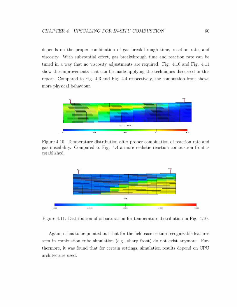
CHAPTER 4. UPSCALING FOR IN-SITU COMBUSTION 60
depends on the proper combination of gas breakthrough time, reaction rate, and
viscosity. With substantial effort, gas breakthrough time and reaction rate can be
tuned in a way that no viscosity adjustments are required. Fig. 4.10 and Fig. 4.11
show the improvements that can be made applying the techniques discussed in this
report. Compared to Fig. 4.3 and Fig. 4.4 respectively, the combustion front shows
more physical behaviour.
Figure 4.10: Temperature distribution after proper combination of reaction rate andgas miscibility. Compared to Fig. 4.4 a more realistic reaction combustion front isestablished.
Figure 4.11: Distribution of oil saturation for temperature distribution in Fig. 4.10.
Again, it has to be pointed out that for the field case certain recognizable features
seen in combustion tube simulation (e.g. sharp front) do not exist anymore. Fur-
thermore, it was found that for certain settings, simulation results depend on CPU
architecture used.
Chapter 5
Discussion and Conclusion
This master thesis summarizes the experimental efforts undertaken to describe the
characteristics of a Central European crude oil with respect to the process of ISC.
Combining RTO experiments with the isoconversional principle, apparent activation
energy values were determined for several surface area cases. Iscoconversional results
clearly show the impact of reduced surface area. Overall, reduction in surface area
results in an increase of apparent activation energy for both LTO and HTO reactions.
Using plots of activation energy versus temperature aids the derivation of customized
reaction schemes ([15]) and allows the introduction of special characteristics that
general purpose reaction schemes might not be able to cover. For the crude oil under
investigation, a reaction scheme is currently in preparation. A major issue is how
to model the local maximum right before the Death Valley (e.g. see Fig. 2.8) that
apparently is an important characteristic of the crude oil. Narrow confidence bands for
apparent activation energy illustrate little random error. Overall, the crude oil/rock
combination shows good kinetics and a high tolerance regarding reduced surface area.
Combustion tube temperature profiles exhibit heating rates in the range of 10◦C/min
to 25◦C/min, depending on the oil used. Also, before the combustion front arrives at
a certain differential volume in the tube, this volume was already brought to steam
temperature allowing volatile elements in the oil to evaporate. The questions are
will behavior have an impact on governing reactions and do the apparent activa-
tion energies depend on heating rates. It is necessary, therefore, to apply a heating
61
CHAPTER 5. DISCUSSION AND CONCLUSION 62
scheme that resembles the combustion tube temperature profiles more accurately if
these questions are to be answered. In short, the sample in the kinetic cell should
first be heated up to steam temperature. The temperature is then held constant for
a certain amount of time to mimic the temperature history in the combustion tube.
Finally, a heating rate in accordance with combustion tube heating rates is applied.
The isoconversional principle can be applied as usual because a linear heating history
is not needed. For the field it is believed that heating rates are more in the range of
2◦C/min ([22]). Hence, except for the preheating of the oil, heating rates do not need
to be changed.
Another question is if a different span of heating rates should be used e.g. instead
of heating rates from 1◦C/min to 2◦C/min with 0.2◦C/min increments we could use
a range of 1◦C/min to 20◦C/min with 4◦C/min increments. It is still under debate to
which extent the isoconversional principle requires heating rates close to each other.
The isoconversional method is a comparably young method for analysis of ISC and
we still need to unlock its full potential. For example isoconversion based on carbon
dioxide production.
The effect of surface area was also noticeable for combustion tube runs. The tube
run having the smallest surface area died. For the second run with reduced surface
area an increased fuel consumption was calculated. At the same time, however, this
run yielded the greatest recovery. The reason is, that in the tube several driving
mechanisms need to be taken into account. The decrease in surface area - that
is especially true when removing the clay - went hand in hand with an increase in
permeability. Hence, gravity drainage and gases flushing the tube added substantially
to the production. Recovery values from tube runs cannot be directly related to the
field case. We must take into account both the different driving mechanisms and
also the permeability of the sand pack is likely to be greater compared to the field.
Permeability for the sand pack was determined to be in the range of 10 mD. Also,
the H/C Ratio was the largest for the successful runs, indicating problems sustaining
the front in the HTO region.
A significant air flow rate is crucial in order to sustain the combustion tube front.
In Fig. 3.23, we saw that with decreasing air flow rate, the burning process shifts
CHAPTER 5. DISCUSSION AND CONCLUSION 63
from an HTO dominated regime (low H/C-ratio) into an LTO dominated regime
(high H/C-ratio). For the field case, air flow rates are of great importance because
they dictate economics to a great extent. If flow rates are too large, a lot of air
and, therefore, compressor capacity is wasted. In addition, air breakthrough at the
producer poses a safety hazard. Also, in order to sustain the combustion front, not
all of the coke created needs to be burned. Low flow rates cause a shift from the HTO
regime to the LTO regime to a point where the front cannot be sustained.
Regarding flue gas oscillations, we see a direct impact of air flow rate. Oscillations
disappeared with decreasing air flow rate. Tracking the H/C-ratio over time the fuel
laid down in the presence of air differs from from the fuel created in an oxygen deficient
environment.
Specific conclusions from this study follow.
• Kinetic measurements interpreted using the isoconversional approach appear to
be predictive of combustion tube success and are able to quantify the shift in
kinetics as the surface area changes.
• Effluent gas composition oscillation measured during combustion tube experi-
ments are shown to originate from both flow rate and packing heterogeneities.
• The H/C ratio reported for successful combustion tube runs ranges from 1.25
to 1.86 suggesting an HTO dominated regime, as do the peak temperatures
measured.
• Air requirements for larger surface area experiments are calculated to be around
250 m3(ST )/m3. With decreased surface area an increase of air requirements
up to 337 m3(ST )/m3 was observed.
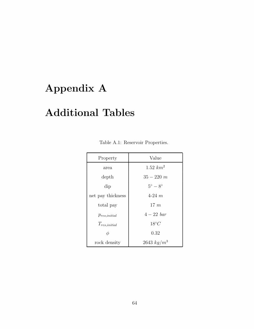
Appendix A
Additional Tables
Table A.1: Reservoir Properties.
Property Value
area 1.52 km2
depth 35− 220 m
dip 5◦ − 8◦
net pay thickness 4-24 m
total pay 17 m
pres,initial 4− 22 bar
Tres,initial 18◦C
φ 0.32
rock density 2643 kg/m3
64
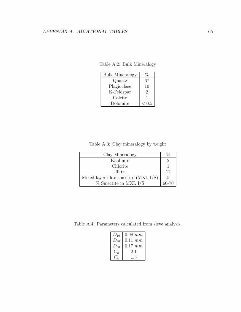
APPENDIX A. ADDITIONAL TABLES 65
Table A.2: Bulk Mineralogy
Bulk Mineralogy %Quartz 67
Plagioclase 10K-Feldspar 2Calcite 1Dolomite < 0.5
Table A.3: Clay mineralogy by weight
Clay Mineralogy %Kaolinite 2Chlorite 1Illite 12
Mixed-layer illite-smectite (MXL I/S) 5% Smectite in MXL I/S 60-70
Table A.4: Parameters calculated from sieve analysis.
D10 0.08 mmD30 0.11 mmD60 0.17 mmCu 2.1Cc 1.5
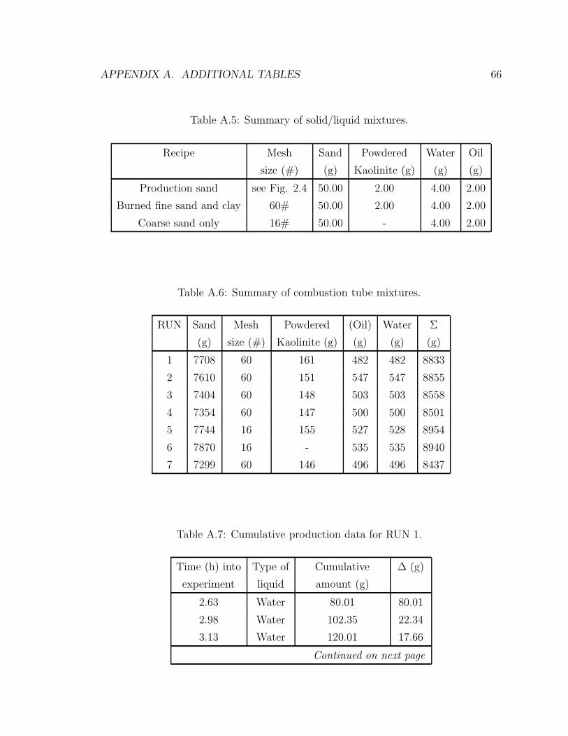
APPENDIX A. ADDITIONAL TABLES 66
Table A.5: Summary of solid/liquid mixtures.
Recipe Mesh Sand Powdered Water Oil
size (#) (g) Kaolinite (g) (g) (g)
Production sand see Fig. 2.4 50.00 2.00 4.00 2.00
Burned fine sand and clay 60# 50.00 2.00 4.00 2.00
Coarse sand only 16# 50.00 - 4.00 2.00
Table A.6: Summary of combustion tube mixtures.
RUN Sand Mesh Powdered (Oil) Water Σ
(g) size (#) Kaolinite (g) (g) (g) (g)
1 7708 60 161 482 482 8833
2 7610 60 151 547 547 8855
3 7404 60 148 503 503 8558
4 7354 60 147 500 500 8501
5 7744 16 155 527 528 8954
6 7870 16 - 535 535 8940
7 7299 60 146 496 496 8437
Table A.7: Cumulative production data for RUN 1.
Time (h) into Type of Cumulative ∆ (g)
experiment liquid amount (g)
2.63 Water 80.01 80.01
2.98 Water 102.35 22.34
3.13 Water 120.01 17.66
Continued on next page
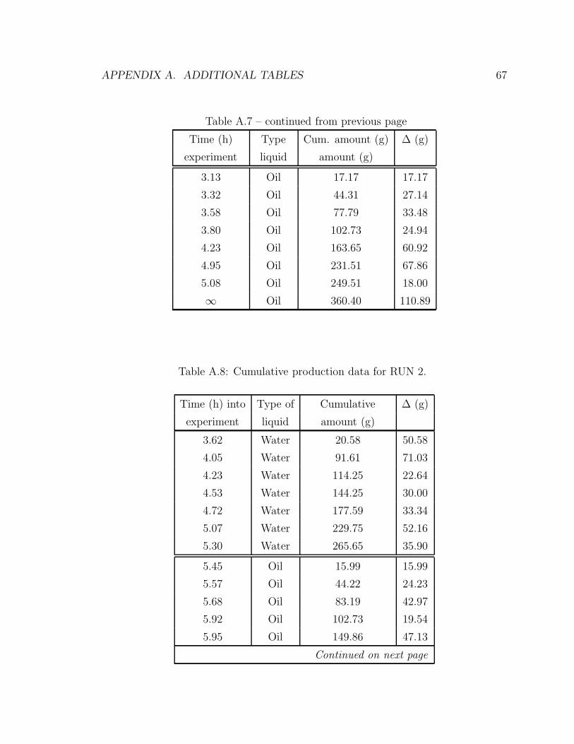
APPENDIX A. ADDITIONAL TABLES 67
Table A.7 – continued from previous page
Time (h) Type Cum. amount (g) ∆ (g)
experiment liquid amount (g)
3.13 Oil 17.17 17.17
3.32 Oil 44.31 27.14
3.58 Oil 77.79 33.48
3.80 Oil 102.73 24.94
4.23 Oil 163.65 60.92
4.95 Oil 231.51 67.86
5.08 Oil 249.51 18.00
∞ Oil 360.40 110.89
Table A.8: Cumulative production data for RUN 2.
Time (h) into Type of Cumulative ∆ (g)
experiment liquid amount (g)
3.62 Water 20.58 50.58
4.05 Water 91.61 71.03
4.23 Water 114.25 22.64
4.53 Water 144.25 30.00
4.72 Water 177.59 33.34
5.07 Water 229.75 52.16
5.30 Water 265.65 35.90
5.45 Oil 15.99 15.99
5.57 Oil 44.22 24.23
5.68 Oil 83.19 42.97
5.92 Oil 102.73 19.54
5.95 Oil 149.86 47.13
Continued on next page
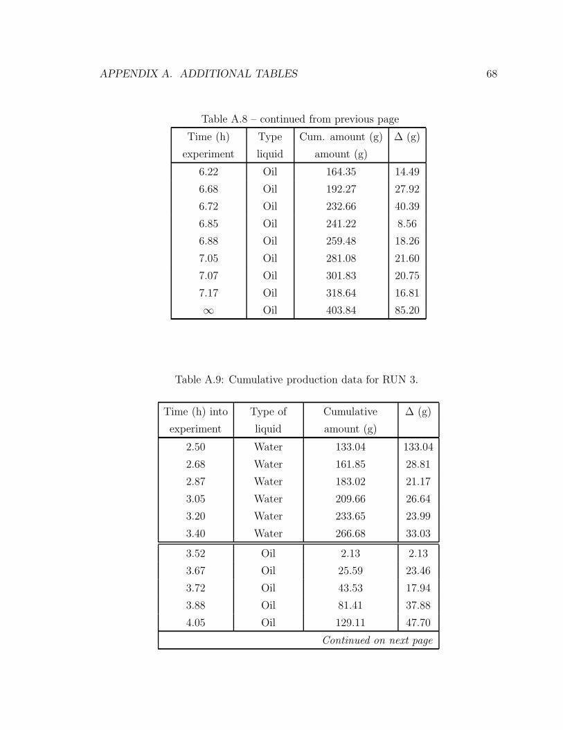
APPENDIX A. ADDITIONAL TABLES 68
Table A.8 – continued from previous page
Time (h) Type Cum. amount (g) ∆ (g)
experiment liquid amount (g)
6.22 Oil 164.35 14.49
6.68 Oil 192.27 27.92
6.72 Oil 232.66 40.39
6.85 Oil 241.22 8.56
6.88 Oil 259.48 18.26
7.05 Oil 281.08 21.60
7.07 Oil 301.83 20.75
7.17 Oil 318.64 16.81
∞ Oil 403.84 85.20
Table A.9: Cumulative production data for RUN 3.
Time (h) into Type of Cumulative ∆ (g)
experiment liquid amount (g)
2.50 Water 133.04 133.04
2.68 Water 161.85 28.81
2.87 Water 183.02 21.17
3.05 Water 209.66 26.64
3.20 Water 233.65 23.99
3.40 Water 266.68 33.03
3.52 Oil 2.13 2.13
3.67 Oil 25.59 23.46
3.72 Oil 43.53 17.94
3.88 Oil 81.41 37.88
4.05 Oil 129.11 47.70
Continued on next page
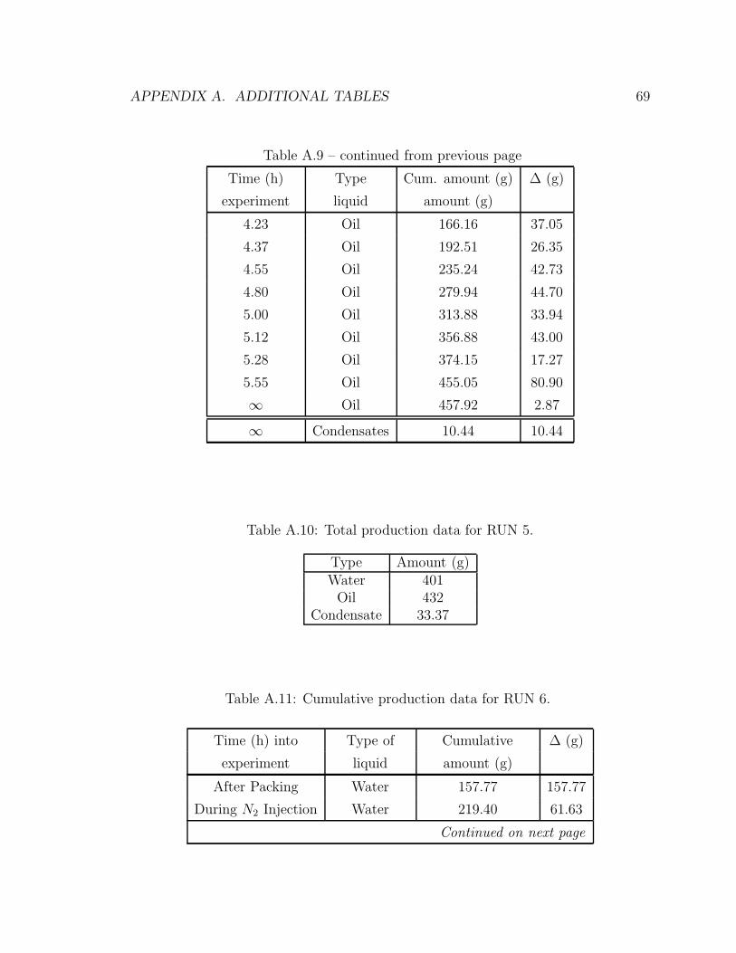
APPENDIX A. ADDITIONAL TABLES 69
Table A.9 – continued from previous page
Time (h) Type Cum. amount (g) ∆ (g)
experiment liquid amount (g)
4.23 Oil 166.16 37.05
4.37 Oil 192.51 26.35
4.55 Oil 235.24 42.73
4.80 Oil 279.94 44.70
5.00 Oil 313.88 33.94
5.12 Oil 356.88 43.00
5.28 Oil 374.15 17.27
5.55 Oil 455.05 80.90
∞ Oil 457.92 2.87
∞ Condensates 10.44 10.44
Table A.10: Total production data for RUN 5.
Type Amount (g)Water 401Oil 432
Condensate 33.37
Table A.11: Cumulative production data for RUN 6.
Time (h) into Type of Cumulative ∆ (g)
experiment liquid amount (g)
After Packing Water 157.77 157.77
During N2 Injection Water 219.40 61.63
Continued on next page
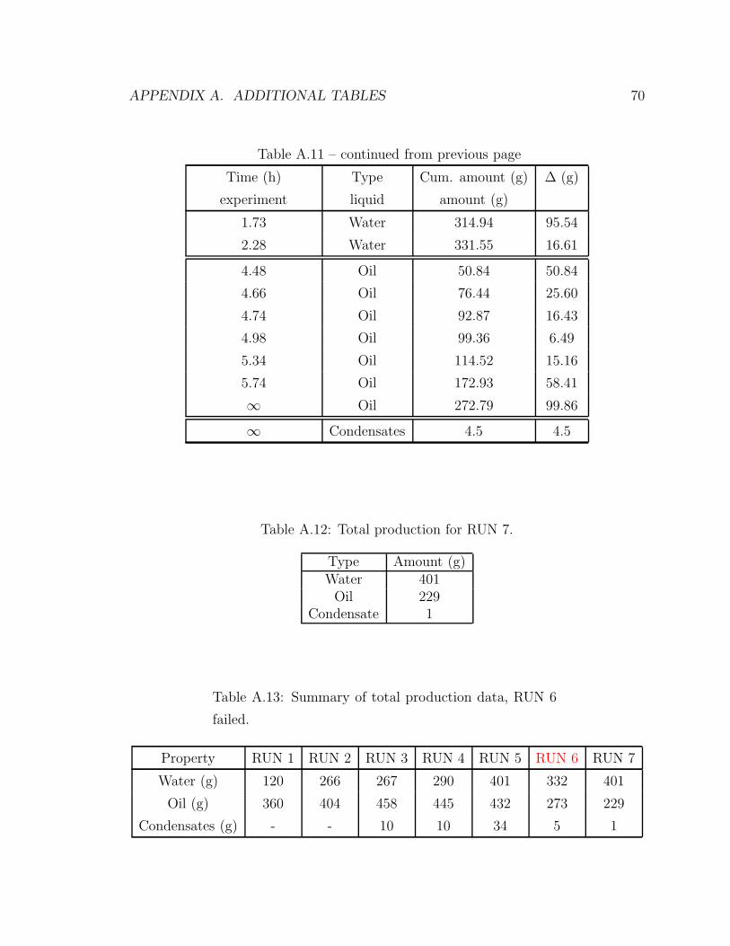
APPENDIX A. ADDITIONAL TABLES 70
Table A.11 – continued from previous page
Time (h) Type Cum. amount (g) ∆ (g)
experiment liquid amount (g)
1.73 Water 314.94 95.54
2.28 Water 331.55 16.61
4.48 Oil 50.84 50.84
4.66 Oil 76.44 25.60
4.74 Oil 92.87 16.43
4.98 Oil 99.36 6.49
5.34 Oil 114.52 15.16
5.74 Oil 172.93 58.41
∞ Oil 272.79 99.86
∞ Condensates 4.5 4.5
Table A.12: Total production for RUN 7.
Type Amount (g)Water 401Oil 229
Condensate 1
Table A.13: Summary of total production data, RUN 6
failed.
Property RUN 1 RUN 2 RUN 3 RUN 4 RUN 5 RUN 6 RUN 7
Water (g) 120 266 267 290 401 332 401
Oil (g) 360 404 458 445 432 273 229
Condensates (g) - - 10 10 34 5 1

APPENDIX A. ADDITIONAL TABLES 71
Table A.14: Summary of stoichiometry for HTO reaction, see Eqn. 3.1.
RUN H/C O2 N2 CO2 CO O2 H2O N2
1 1.25 1.48 5.67 0.75 0.25 0.29 0.63 5.672 1.26 1.41 5.41 0.74 0.26 0.23 0.63 5.413 1.86 2.65 5.97 0.75 0.25 0.25 0.93 5.974 1.37 1.41 5.42 0.74 0.26 0.20 0.69 5.425 1.42 1.38 5.28 0.71 0.29 0.17 0.71 5.286 2.18 18.26 69.97 0.68 0.32 16.88 1.09 69.977 1.45 1.26 4.84 0.75 0.25 0.02 0.72 4.84
Table A.15: Summary of operational data, RUN 6 failed.
Property RUN 1 RUN 2 RUN 3 RUN 4 RUN 5 RUN 6 RUN 7
Oil Recovery (%) 87 92 93 90 98 82 54
Fuel consumed (g) 58 68 63 65 76 16 59
Overall H/C ratio 1.38 1.38 1.45 1.47 1.54 2.78 1.50
Fuel requirements (kg/m3) 18.8 23.2 19.6 19.8 27.2 7.8 21.1
Fuel requirements (kg fuel/100 kg sand) 0.76 0.89 0.85 0.88 0.99 0.2 0.81
Air requirements (m3(ST )/m3) 248 291 250 244 337 406 236
Table A.16: Summary of gas phase parameters, RUN 6
failed.
Property RUN 1 RUN 2 RUN 3 RUN 4 RUN 5 RUN 6 RUN 7
H/C ratio 1.25 1.26 1.86 1.37 1.42 2.18 1.45
OFR (m3(ST )/m3) 2.64 2.51 2.65 2.50 2.43 30.38 2.22
AFR (m3(ST )/m3) 12.74 12.14 12.82 12.06 11.72 146.78 10.71
fO2R 0.74 0.73 0.65 0.72 0.71 0.61 0.71
Excess O2 0.2 0.16 0.14 0.14 0.12 0.92 0.02
Excess air 0.25 0.19 0.16 0.17 0.14 - 0.02
m 3.03 2.87 3.02 2.85 2.41 2.12 3.07
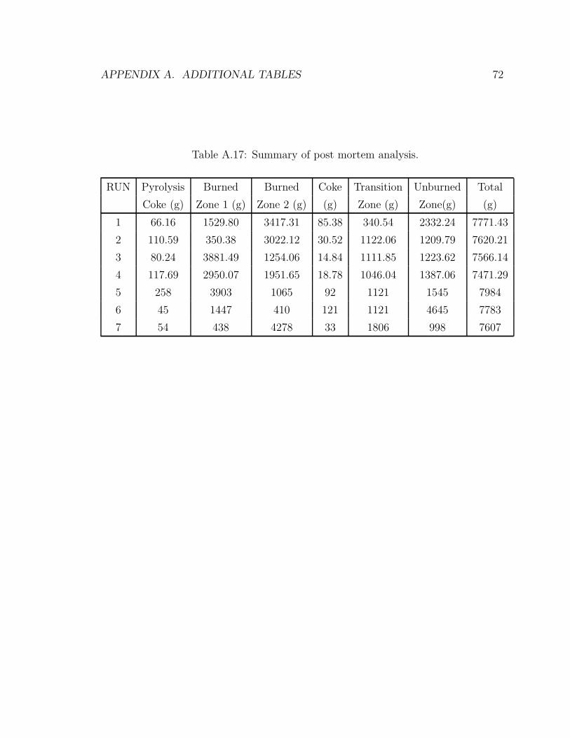
APPENDIX A. ADDITIONAL TABLES 72
Table A.17: Summary of post mortem analysis.
RUN Pyrolysis Burned Burned Coke Transition Unburned Total
Coke (g) Zone 1 (g) Zone 2 (g) (g) Zone (g) Zone(g) (g)
1 66.16 1529.80 3417.31 85.38 340.54 2332.24 7771.43
2 110.59 350.38 3022.12 30.52 1122.06 1209.79 7620.21
3 80.24 3881.49 1254.06 14.84 1111.85 1223.62 7566.14
4 117.69 2950.07 1951.65 18.78 1046.04 1387.06 7471.29
5 258 3903 1065 92 1121 1545 7984
6 45 1447 410 121 1121 4645 7783
7 54 438 4278 33 1806 998 7607
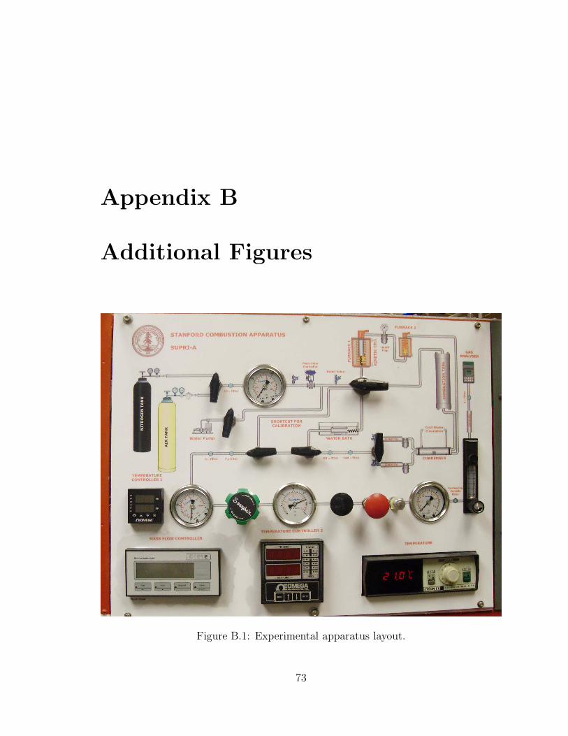
Appendix B
Additional Figures
Figure B.1: Experimental apparatus layout.
73
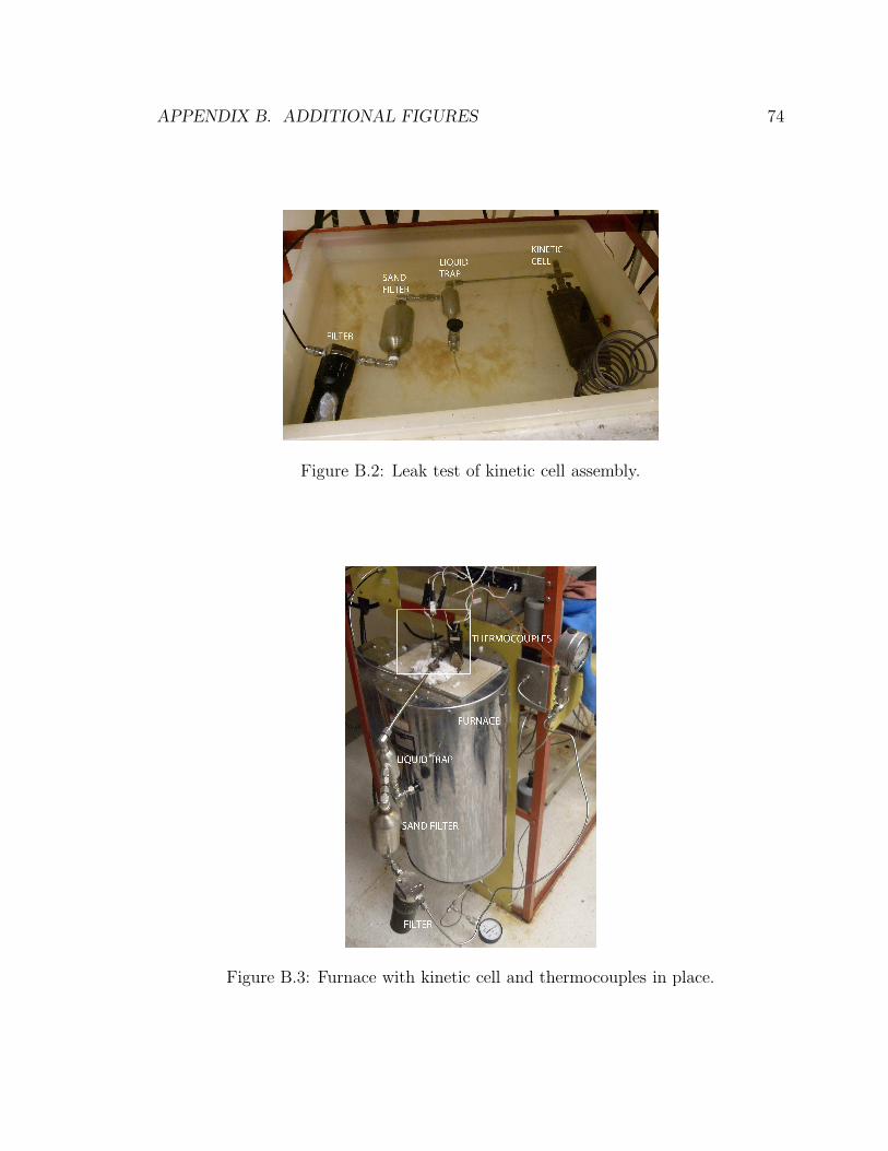
APPENDIX B. ADDITIONAL FIGURES 74
Figure B.2: Leak test of kinetic cell assembly.
Figure B.3: Furnace with kinetic cell and thermocouples in place.
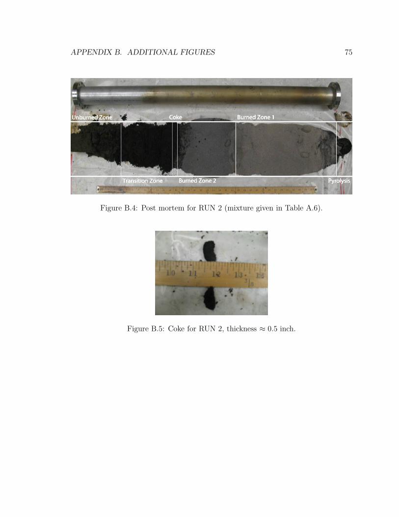
APPENDIX B. ADDITIONAL FIGURES 75
Figure B.4: Post mortem for RUN 2 (mixture given in Table A.6).
Figure B.5: Coke for RUN 2, thickness ≈ 0.5 inch.
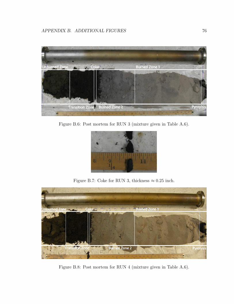
APPENDIX B. ADDITIONAL FIGURES 76
Figure B.6: Post mortem for RUN 3 (mixture given in Table A.6).
Figure B.7: Coke for RUN 3, thickness ≈ 0.25 inch.
Figure B.8: Post mortem for RUN 4 (mixture given in Table A.6).
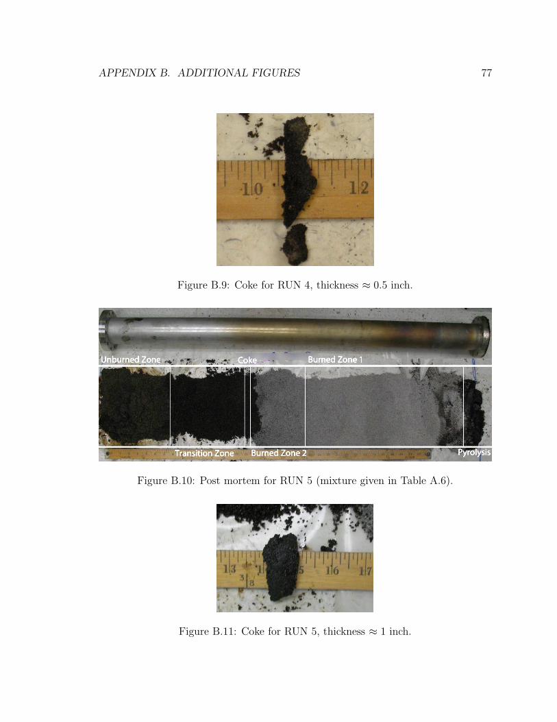
APPENDIX B. ADDITIONAL FIGURES 77
Figure B.9: Coke for RUN 4, thickness ≈ 0.5 inch.
Figure B.10: Post mortem for RUN 5 (mixture given in Table A.6).
Figure B.11: Coke for RUN 5, thickness ≈ 1 inch.
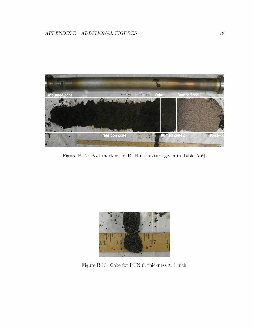
APPENDIX B. ADDITIONAL FIGURES 78
Figure B.12: Post mortem for RUN 6 (mixture given in Table A.6).
Figure B.13: Coke for RUN 6, thickness ≈ 1 inch.
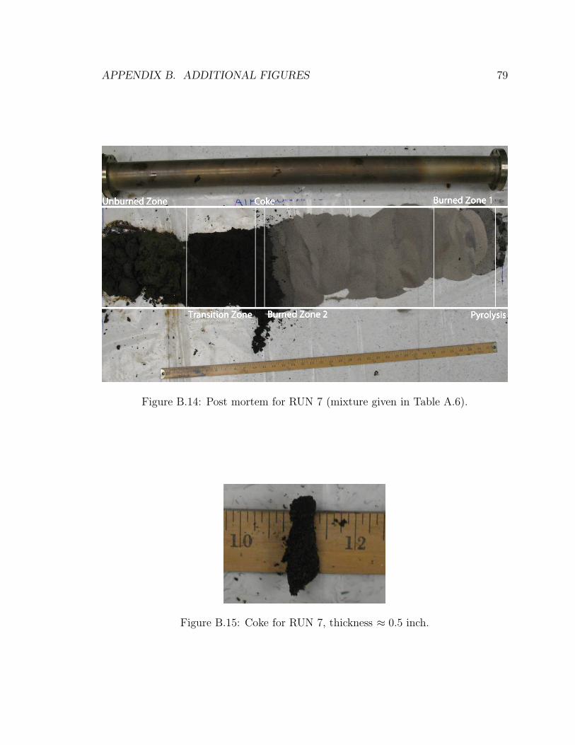
APPENDIX B. ADDITIONAL FIGURES 79
Figure B.14: Post mortem for RUN 7 (mixture given in Table A.6).
Figure B.15: Coke for RUN 7, thickness ≈ 0.5 inch.
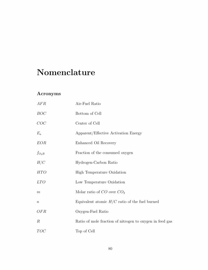
Nomenclature
Acronyms
AFR Air-Fuel Ratio
BOC Bottom of Cell
COC Center of Cell
Ea Apparent/Effective Activation Energy
EOR Enhanced Oil Recovery
fO2R Fraction of the consumed oxygen
H/C Hydrogen-Carbon Ratio
HTO High Temperature Oxidation
LTO Low Temperature Oxidation
m Molar ratio of CO over CO2
n Equivalent atomic H/C ratio of the fuel burned
OFR Oxygen-Fuel Ratio
R Ratio of mole fraction of nitrogen to oxygen in feed gas
TOC Top of Cell
80
Bibliography
[1] Al-Saffar, H., Price, D., Soufi, A., Hughes, R., Distinguishing between overlapping
low temperature and high temperature oxidation data obtained from a pressurised
flow reactor system using consolidated core material. Fuel, Volume 79, Issue 7,
May 2000, Pages 723-732, ISSN 0016-2361, DOI: 10.1016/S0016-2361(99)00210-
0.
[2] Ambalea, A. M., Freitag, N. Thermogravimetric studies on pyrolysis and combus-
tion behaviour of a heavy oil and its asphaltenes. Energy Fuels 2006, 20, 560565.
[3] Bazargan M., Chen B., Cinar M., Glatz G., Lapene A., Zhu Z., Castanier L.,
Gerritsen M., and Kovscek A. 2011. A Combined Experimental and Simulation
Workflow to Improve Predictability of In Situ Combustion. SPE 144599 presented
at the SPE Western Regional Meeting, Society of Petroleum Engineers.
[4] Benham, A. L., Poettman, F. H. The Thermal Recovery Process - An Analysis
of Laboratory Combustion Data. Journal of Petroleum Technology, Volume 10,
Number 9, 1958, 83-85.
[5] Bousaid, I. S., Ramey, H. J., Jr. Oxidation of crude oil in porous media. Soc.
Pet. Eng. J. 1968, 137148.
[6] Burger, J.G., Chemical Aspects of In-Situ Combustion - Heat of Combustion
and Kinetics. Institut Francais Du Petrole, SPE Journal, Volume 12, Number 5,
October 1972, pp. 410-422.
[7] Burger, J., Sourrieau P., and Combarnous M., Thermal Recovery Methods. Edi-
tions TECHNIP, Paris France, 1984.
81
BIBLIOGRAPHY 82
[8] Butler, R.M., Thermal Recovery of Oil and Bitumen. Prentice Hall, Englewood
Cliffs, New Jersey, 1991.
[9] Burnham, A. K., Dinh, L. N., A comparison of isoconversional and model-fitting
approaches to kinetic parameter estimation and application predictions. J. Therm.
Anal. Calorim. 2007, 89, pp. 479490.
[10] Carcoana, A. Results and Difficulties of the World’s Largest In-Situ Combustion
Process: Suplacu de Barcau Field, Romania. SPE/DOE Enhanced Oil Recovery
Symposium, Tulsa, Oklahoma, April 1990.
[11] Carberry, J. J. Chemical and Catalytic Reaction Engineering, McGraw-Hill Book
Company, New York, 1976.
[12] M. Cinar, L.M. Castanier, and A.R. Kovscek, 2009. Isoconversional Kinetic Anal-
ysis of the Combustion of Heavy Hydrocarbons. SPE Western Regional Meeting,
24-26 March 2009, San Jose, California.
[13] Cinar, M., Castanier, L. M., Kovscek, A. R., Improved analysis of the kinetics
of crude-oil in-situ combustion. In SPE Western Regional Meeting 2008, Bakers-
field, CA, March 31-April 2, 2008; SPE Paper 113948.
[14] Cinar, M., Castanier, L.M., and Kovscek, A.R., 2011. Predictability of Crude Oil
In-Situ Combustion by the Isoconversional Kinetic Approach. To be published in
SPE Journal, 2011.
[15] Cinar, M., Castanier, L.M., and Kovscek, A.R., 2011. Combustion Kinetics of
Heavy Oils in Porous Media. Energy and Fuels, submitted May 2011.
[16] Coats, K. H., In-situ combustion model, Soc. Pet. Eng. J., Dec. 1980, 533554.
[17] Coats K.H. 1983. Some Observations on Field-Scale Simulation of the In-Situ
Combustion Process. SPE12247 presented at the SPE Reservoir Simulation Sym-
posium, Society of Petroleum Engineers.
BIBLIOGRAPHY 83
[18] Dechelette B., Heugas O., Quenault G., Bothua J., and Christensen J. 2006. Air
Injection-Improved Determination of the Reaction Scheme with Ramped Tem-
perature Experiment and Numerical Simulation. Journal of Canadian Petroleum
Technology 45(1).
[19] Ewing R. Richard, The Mathematics of Reservoir Simulation, Society for Indus-
trial Mathematics (January 1, 1987).
[20] Farouq Ali, S.M., A Current Appraisal of In-Situ Combustion Field Tests. Jour-
nal of Petroleum Technology, Volume 24, Number 4, 1972, pp. 477-486.
[21] Fassihi, M.R., W.E. Brigham, and H.J. Ramsey Jr. 1984. Reaction Kinetics of
In Situ Combustion: Part 1 Observation, Part 2 Modelling. Sot. of Pet. Eng. J.
Vol. 24, No. 4, pp. 399416.
[22] Fassihi, M. R. Analysis of fuel oxidation in in-situ combustion oil recovery. Ph.D.
dissertation, Stanford University, Stanford, CA, April 1981.
[23] Friedman, H. L. Kinetics of thermal degradation. J. Polym. Sci., Part C: Polym.
Lett. 1964, 6, 183195.
[24] Galwey, A.K., What is meant by the term ‘variable activation energy’ when ap-
plied in the kinetic analyses of solid state decompositions (crystolysis reactions)?.
Thermochimica Acta, Volume 397, Issues 1-2, 21 February 2003, Pages 249-268,
ISSN 0040-6031, DOI: 10.1016/S0040-6031(02)00271-X.
[25] Gates C.F. and Ramey H.J. 1980. A Method for Engineering In-Situ Combustion
Oil Recovery Projects. Journal of Petroleum Technology 32(2): 285-294.
[26] Christensen J., Darche G., Dechelette B., Ma H., and Sammon P. 2004. Appli-
cations of Dynamic Gridding To Thermal Simulations. SPE 86969 presented at
SPE International Thermal Operations and Heavy Oil Symposium and Western
Regional Meeting, Society of Petroleum Engineers.
BIBLIOGRAPHY 84
[27] Glatz G., Stanford University, Hascakir B., Stanford University, Castanier L.M.,
Stanford University, Clemens T., OMV, Kovscek A.R., Stanford University. Ki-
netic Cell and Combustion Tube Results for a Central European Crude. SPE
146089-MS, SPE Annual Technical Conference and Exhibition, 30 October-2
November 2011, Denver, Colorado, USA.
[28] Gutierrez D., Skoreyko F., Moore R.G., Mehta S.A., and Ursenbach M.G. 2009.
The Challenge of Predicting Field Performance of Air Injection Projects Based
on Laboratory and Numerical Modelling. Journal of Canadian Petroleum Tech-
nology 48(4): 23-33.
[29] Genrich, J.F., Sohio Petroleum Co.; Pope, G.A., U. of Texas, A Simplified
Performance-Predictive Model for In-Situ Combustion Processes. SPE Reservoir
Engineering, Volume 3, Number 2, 1988, pp. 410-418.
[30] Hascakir, B., Glatz, G., Castanier, L.M., and Kovscek, A.R., 2011. In-Situ Com-
bustion Dynamics Visualized With X-Ray Computed Tomography. SPE J. SPE-
135186-PA.
[31] Hundsdorfer W., Jan G. Verwer, Numerical Solutions of Time-Dependent
Advection-Diffusion-Reaction Equations, Springer 2007.
[32] International Energy Outlook, Report: DOE/EIA-0484(2010),
http://www.eia.doe.gov/oiaf/ieo/, 2010.
[33] Kristensen M.R. 2008. Development of Models and Algorithms for the Study of
Reactive Porous Media Processes. Ph.D. thesis, Technical University of Denmark.
[34] Mamora, D.D., 1993. Kinetics of in-situ combustion. Ph.D. Thesis, Stanford,
CA: Stanford University.
[35] Mamora, D.D., New Findings in Low-Temperature Oxidation of Crude Oil. SPE
293-24, March, 1995.
BIBLIOGRAPHY 85
[36] Marjerrison D. and Fassihi M. 1992. A Procedure for Scaling Heavy-Oil Com-
bustion Tube Results to a Field Model. SPE 24175 presented at the SPE/DOE
Enhanced Oil Recovery Symposium, Society of Petroleum Engineers.
[37] Moore, R.G., New Strategies for In-Situ Combustion. J. Can. Pet. Tech., Vol.32,
No. 10, December, pp. 11-13.
[38] Moore, R.G., Ursenbach, M.G., Laureshen, C.J., and Mehta, S.A., 1997. Obser-
vation and Design Considerations for In-Situ Combustion. SPE, 97-100.
[39] Moore, R.G., Laureshen, C.J., Ursenbach, M.G., Mehta,, S.A., Belgrave, J.D.M.,
U. of Calgary, Combustion/Oxidation Behavior of Athabasca Oil Sands Bitumen.
SPE Reservoir Evaluation & Engineering, Volume 2, Number 6, December 1999,
pp. 565-571.
[40] Morten, R. K., Development of Models and Algorithms for the Study of Re-
active Porous Media Processes, Technical University of Denmark, Department
of Chemical and Biochemical Engineering, Frydenberg A/S, Copenhagen, Den-
mark, 2008.
[41] Oyekonwu, M.O., Pande, K., Ramey, H.J., and Brigham, W. E., 1986. Experi-
mental and simulation studies of laboratory in-situ combustion recovery. Paper
SPE 15090, SPE 56th California Regional Meeting, Oakland, CA, April 2-4, pp.
483-496.
[42] Paduraru, R., Pantazi, I. IOR/EOR - Over Six Decades of Romanian Experi-
ence, Institute for Research and Technology (ICPT), SPE European Petroleum
Conference, Paris, France, October 2000.
[43] Prasad, R. S., Slater, J. A. High Pressure Combustion Tube Tests, SPE/DOE
14919, Presented at the 5th SPE/DOE Symposium on Enhanced Oil Recovery.
Tulsa, Oklahoma, April 20-23, 1986
[44] Prats, M., Thermal recovery, Henry L. Doherty Series, monograph vol. 7, SPE,
1986.

BIBLIOGRAPHY 86
[45] Petit, H.J-M., Le Thiez, P., Lemonnier, P., History Matching of a Heavy-Oil
Combustion Pilot in Romania. SPE/DOE Enhanced Oil Recovery Symposium,
Tulsa, Oklahoma, April 1990.
[46] Ren, S. R., Greaves, M., Rathbone, R. R., An IOR Technique for Light-Oil
Reservoirs, SPE Journal, Volume 7, Number 1, pp. 90-99, March 2002.
[47] Rubin, Barry, Buchanan, W. Lloyd, Computer Modelling Group, 1985.A General
Purpose Thermal Model. SPE Journal, Volume 25, Number 2, 202-214.
[48] Sarathi, P. In-Situ Combustion Handbook Principles and Practices ; National
Petroleum Technology Office: Tulsa, OK, 1999; Report DOE/PC/91008-0374,
OSTI ID 3174.
[49] Savitzky, A., Golay, M. J. E., Smoothing and Differentiation of Data by Simplified
Least Squares Procedures. Analytical Chemistry, Volume 36, Number 8, 1627-
1639, 1964.
[50] Eclipse1 software version 2009 Software Manual. Schlumberger Ltd.
[51] Semenov, N. Chemical Kinetics and Chain Reactions. Oxford University Press:
London, U.K., 1935.
[52] Shirley, D.A., Phys. Rev. B 5, 4709-4714, 1972.
[53] Smith, J. M. Chemical Engineering Kinetics, McGraw-Hill Book Company, New
York, 1970.
[54] Vyazovkin, S., Reply to ”What is meant by the term ’variable activation energy’
when applied in the kinetics analyses of solid state decompositions (crystolysis
reactions)?”. Thermochimica Acta, Volume 397, Number 1, 21 February 2003 ,
pp. 269-271(3).
[55] Wefer G., David Billet, Dierk Hebbeln, Bo B. Jorgensen, Michael Schlter, Tjeerd
C.E. Van Weering. Ocean Margin Systems, Springer; 1 edition (November 4,
2002).
1Mark of Schlumberger
BIBLIOGRAPHY 87
[56] Vyazovkin, S. Isoconversional kinetics in: The handbook of thermal analysis
& calorimetry, Vol.5 Eds. M. E. Brown, P. K. Gallagher, Elsevier, Amsterdam,
2008, pp. 503-538.
[57] Z. Zhu, M. Bazargan, A. Lapene, M. Gerritsen, L. Castanier, and A. Kovscek,
SPE, Stanford University, Upscaling for Field-scale In-situ Combustion Simula-
tion, SPE Western North American Region Meeting, 7-11 May 2011, Anchorage,
Alaska, USA.