towards fully adaptive deep neural networks

Next Generation Wireless S Chen

Towards Fully Adaptive Deep NeuralNetworks

Professor Sheng Chen

School of Electronics and Computer Science

University of Southampton

Southampton SO17 1BJ, United Kingdom

Keynote speech at LSMS2021 & ICSEE2021

October 30 - November 1, Hangzhou, China

Joint work with Dr Tong Liu, Department of Computer Science, University of Sheffield, U.K.

1


Background

• Artificial neural networks have evolved from ‘shallow’ one-hidden-layer architecture,such as RBF, to ‘deep’ architecture

– Deep learning has achieved breakthrough progress in many walks of life– Deep neural networks have been applied to modeling of industrial processes

• Deep learning’s success coincides with digital big data era

– With massive historical data, training of deep neural network models becomespractical

– Enabling the exploitation of deep learning capability to capture complexunderlying nonlinear dynamic behavious from data

• Many real-life processes are not only nonlinear but also highly nonstationary

– During online operation, system’s nonlinear dynamics can change significantly– Deep neural network model must adapt fast to such change

2


Motivations

• Sampling period of many industrial processes is small, and adaptation must besufficiently fast to be completed within a sampling period

– Impossible to adapt structure of deep neural network model, such as SAE,within sampling period

– Instead, adaptation is taken place only on weights of output regression layer– Insufficient for tracking significant and fast changes in system

• We have proposed an adaptive gradient radial basis function network

– Adapting structure of GRBF is not only optimal but also imposes litter onlinecomputation complexity

– Completely feasible to complete adaptation within a sample period– GRBF is a shallow neural network

• Combining deep learning capability of deep neural network, such as SAE, withexcellent adaptability of GRBF? ⇒ Motivate this research

3


System Model

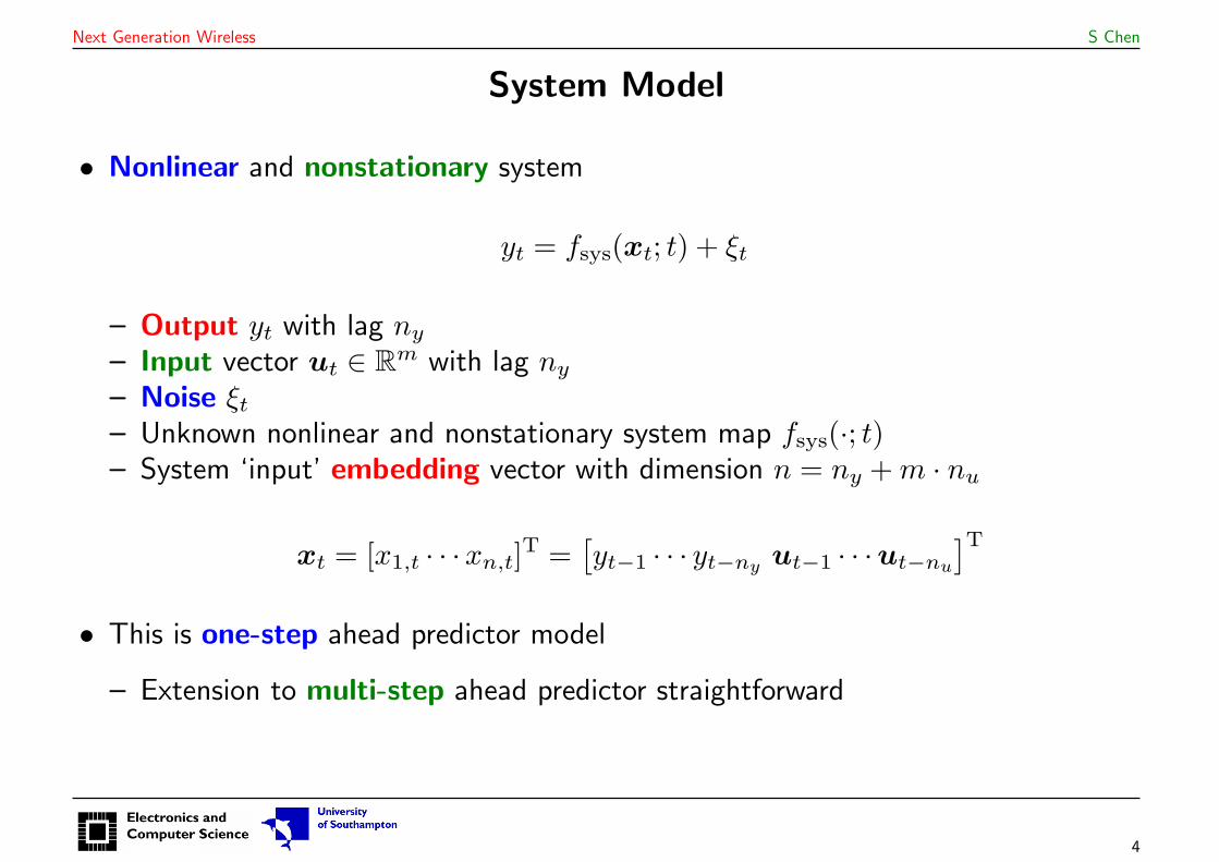
• Nonlinear and nonstationary system

yt = fsys(xt; t) + ξt

– Output yt with lag ny

– Input vector ut ∈ Rm with lag ny

– Noise ξt– Unknown nonlinear and nonstationary system map fsys(·; t)– System ‘input’ embedding vector with dimension n = ny +m · nu

xt = [x1,t · · ·xn,t]T =

[yt−1 · · · yt−ny ut−1 · · ·ut−nu

]T

• This is one-step ahead predictor model

– Extension to multi-step ahead predictor straightforward

4


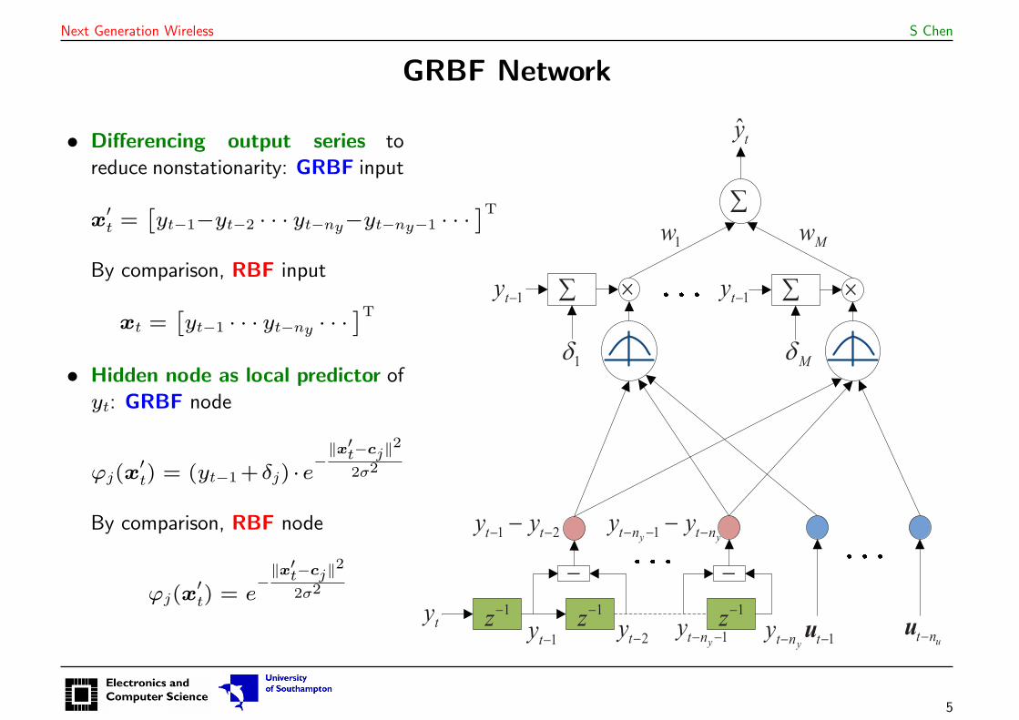
GRBF Network

• Differencing output series to

reduce nonstationarity: GRBF input

x′t =

[

yt−1−yt−2 · · · yt−ny−yt−ny−1 · · ·]T

By comparison, RBF input

xt =[

yt−1 · · · yt−ny · · ·]T

• Hidden node as local predictor of

yt: GRBF node

ϕj(x′t) = (yt−1+δj) ·e

−‖x′t−cj‖

2

2σ2

By comparison, RBF node

ϕj(x′t) = e

−‖x′t−cj‖

2

2σ2

ty ty

ty yt ny

ty

t u ut n u

M

w Mw

z z z

! ! "

!

"

ty

!t ty y

yt ny

y yt n t ny y

ty

5


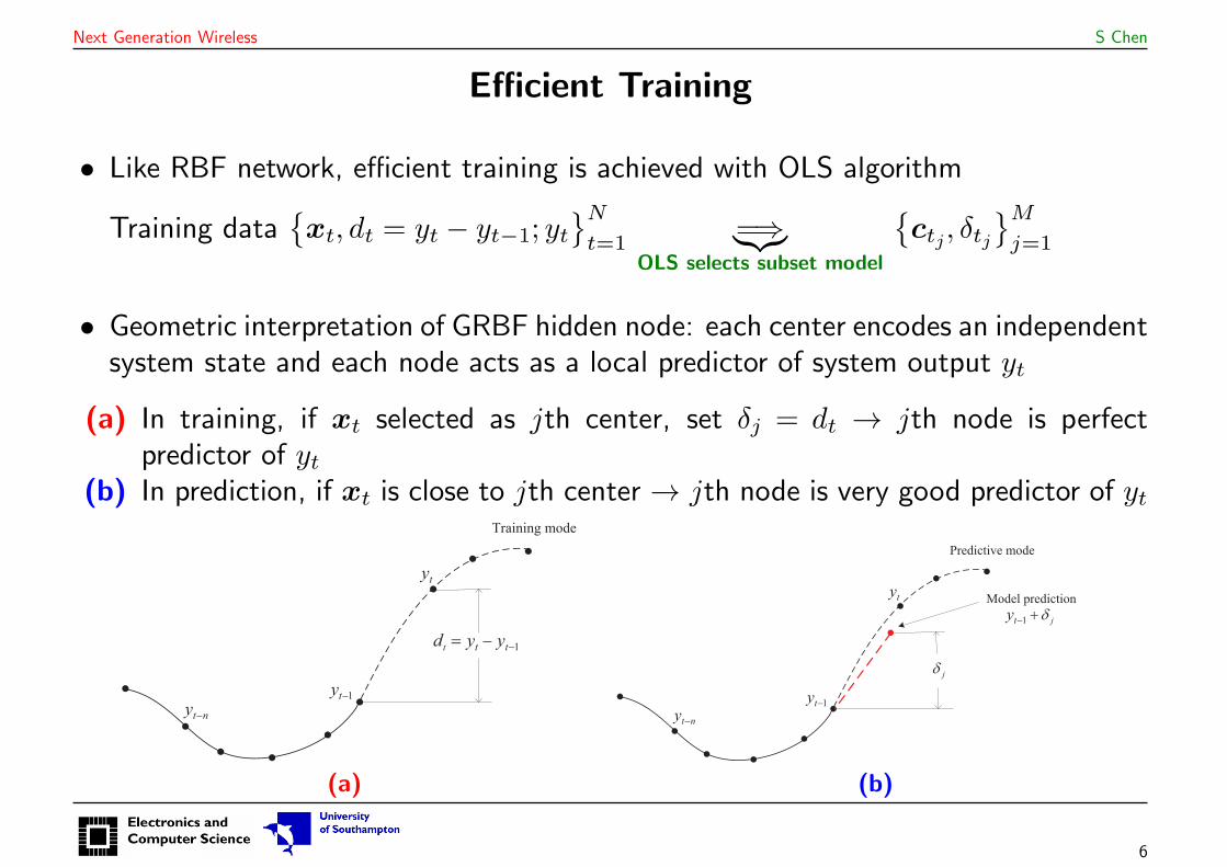
Efficient Training

• Like RBF network, efficient training is achieved with OLS algorithm

Training data{xt, dt = yt − yt−1; yt

}N

t=1=⇒︸︷︷︸

OLS selects subset model

{ctj, δtj

}M

j=1

• Geometric interpretation of GRBF hidden node: each center encodes an independentsystem state and each node acts as a local predictor of system output yt

(a) In training, if xt selected as jth center, set δj = dt → jth node is perfectpredictor of yt

(b) In prediction, if xt is close to jth center → jth node is very good predictor of yt

ty

1ty -

t ny -

1t t td y y-

-=

Training mode

ty

1ty -

t ny -

1 jty d-+

Predictive mode

jd

Model prediction

(a) (b)

6


Online Adaptation

• During online operation, system’s underlying dynamics can change significantly

– A model must adapt to changing operation environment in real time– Optimizing structure of neural networks, both shallow and deep ones, online is

computationally prohibitive

• Typically, when observation/measurement of yt becomes available, RLS is used foronline adaptation of weights of output layer only

– For highly nonstationary process, this is insufficient

• Online learning or adaptive modeling principle: balance ‘stability’ and ‘plasticity’

– Online leaner should have ability to retain acquired knowledge (stability)– At same time, has ability to forget out-of-the-date past knowledge so as to learn

new one as quickly as possible (plasticity)

• Adaptive GRBF achieves balanced or optimal trade-off of stability and plasticity

7


Adaptive GRBF

• During online operation, when current modeling yt is insufficient:

(yt − yt

)2/y2t ≥ thresold

Worst node (smallest squared weighted node output) replaced with a new node:

node center cr ← x′t node scalar δr ← yt − yt−1

– Most nodes do not change - nodes encode independent system states acquiredfrom historical data - stability

– Most out-of-date node is replaced - plasticity, to encode newly emerging systemstate and new node is perfect local predictor of yt

– Online complexity: regularized LS estimation of output layer weights

Liu, Chen, Liang, Du, Harris, “Fast tunable gradient RBF networks for online modeling of

nonlinear and nonstationary dynamic processes,” J. Process Control, 93, 53–65, 2020

8


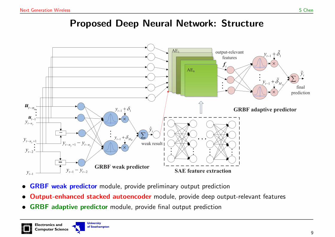
Proposed Deep Neural Network: Structure

ty

yt ny

ty

t u

ut n u

ty

yt ny !

!t ty y

!y yt n t ny y

tf

ty

!

!

! ! ! !

!

!

!"#$%&'($)*&+,-./*

!"#$'+').,0&$)*&+,-./*

123$4&'.5*&$&6.*'-.,/7

!"#$%!&'()

*')+'),%!(!-".)$

/!")'%!&

/0."($

+%!102)0*.

345

34.

5 5ty !"

Wt My !"

#

#

ty

!"

At My

!"

!

• GRBF weak predictor module, provide preliminary output prediction

• Output-enhanced stacked autoencoder module, provide deep output-relevant features

• GRBF adaptive predictor module, provide final output prediction

9


Proposed Deep Neural Network: Rationale

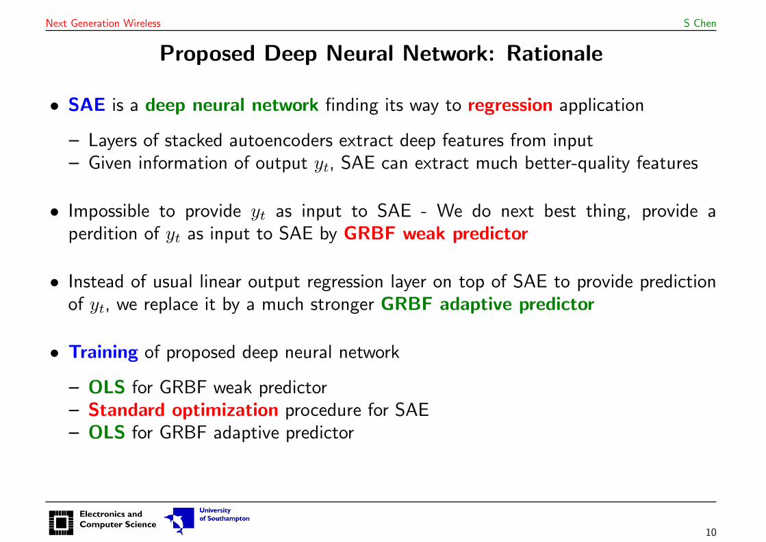
• SAE is a deep neural network finding its way to regression application

– Layers of stacked autoencoders extract deep features from input– Given information of output yt, SAE can extract much better-quality features

• Impossible to provide yt as input to SAE - We do next best thing, provide aperdition of yt as input to SAE by GRBF weak predictor

• Instead of usual linear output regression layer on top of SAE to provide predictionof yt, we replace it by a much stronger GRBF adaptive predictor

• Training of proposed deep neural network

– OLS for GRBF weak predictor– Standard optimization procedure for SAE– OLS for GRBF adaptive predictor

10


Proposed Deep Neural Network: Operation

• Proposed DNN: SAE enhanced by GRBF weak predictor maps process input spaceonto deep feature space, and GRBF adaptive predictor then maps feature spaceonto process output space

• During online operation, GRBF weak predictor and SAE are fixed (impossible toadapt SAE online anyway)

• GRBF adaptive predictor is adapted online to track process’s changing dynamics

– When underlying system dynamics change significant, feature space changesaccordingly

– GRBF adaptive predictor capable of fast adapting to changing process dynamics– while imposing very low online computational complexity, capable of meeting

real-time constraint of small sampling period

• Proposed deep neural network integrates deep learning capability of SAE withexcellent adaptability of GRBF

11


Experiment Setup

• Proposed DNN is compared with following benchmarks

– Long short-term memory (LSTM): during online operation, LSTM is fixed– Stacked autoencoder (SAE): during online operation, SAE is fixed– Adaptive SAE: during online operation, only weights of output regression layer

is adapted by RLS– Adaptive GRBF (AGRBF)

• Performance measure: test mean square error (MSE)

• Online computational complexity: measured by averaged computation time persample (ACTpS) in [ms]

Liu, Tian, Chen, Wang, Harris, “Deep cascade gradient RBF networks with output-relevant

feature extraction and adaptation for nonlinear and nonstationary processes,” submitted to

IEEE Trans. Cybernetics

12


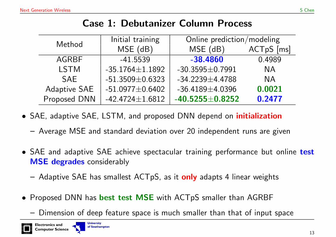
Case 1: Debutanizer Column Process

MethodInitial training Online prediction/modelingMSE (dB) MSE (dB) ACTpS [ms]

AGRBF -41.5539 -38.4860 0.4989LSTM -35.1764±1.1892 -30.3595±0.7991 NASAE -51.3509±0.6323 -34.2239±4.4788 NA

Adaptive SAE -51.0977±0.6402 -36.4189±4.0396 0.0021Proposed DNN -42.4724±1.6812 -40.5255±0.8252 0.2477

• SAE, adaptive SAE, LSTM, and proposed DNN depend on initialization

– Average MSE and standard deviation over 20 independent runs are given

• SAE and adaptive SAE achieve spectacular training performance but online testMSE degrades considerably

– Adaptive SAE has smallest ACTpS, as it only adapts 4 linear weights

• Proposed DNN has best test MSE with ACTpS smaller than AGRBF

– Dimension of deep feature space is much smaller than that of input space

13


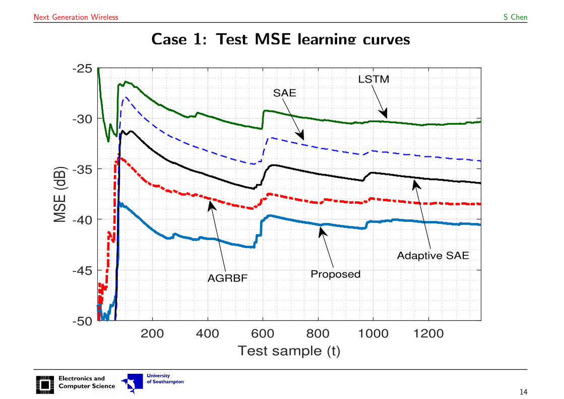
Case 1: Test MSE learning curves

200 400 600 800 1000 1200

Test sample (t)

-50

-45

-40

-35

-30

-25M

SE

(dB

)

Adaptive SAE

ProposedAGRBF

SAE

LSTM

14


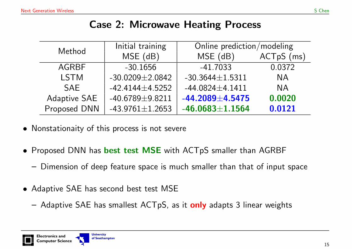
Case 2: Microwave Heating Process

MethodInitial training Online prediction/modelingMSE (dB) MSE (dB) ACTpS (ms)



• Nonstationaity of this process is not severe



• Adaptive SAE has second best test MSE

– Adaptive SAE has smallest ACTpS, as it only adapts 3 linear weights

15


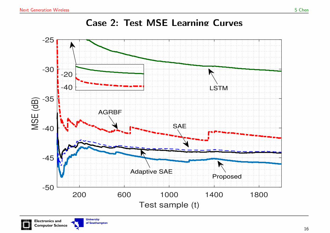
Case 2: Test MSE Learning Curves

200 600 1000 1400 1800

Test sample (t)

-50

-45

-40

-35

-30

-25M

SE

(dB

)

-40

-20

LSTM

AGRBF

SAE

Adaptive SAEProposed

16


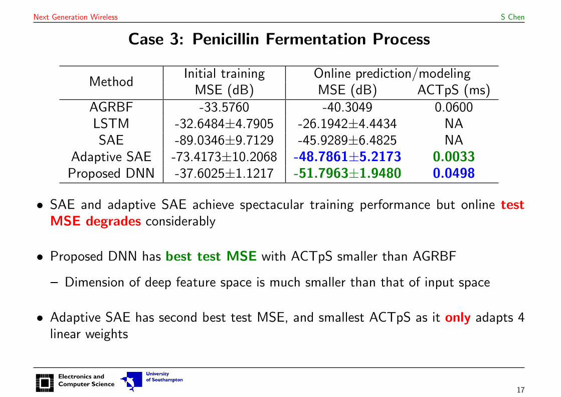
Case 3: Penicillin Fermentation Process

MethodInitial training Online prediction/modelingMSE (dB) MSE (dB) ACTpS (ms)



• SAE and adaptive SAE achieve spectacular training performance but online testMSE degrades considerably



• Adaptive SAE has second best test MSE, and smallest ACTpS as it only adapts 4linear weights

17


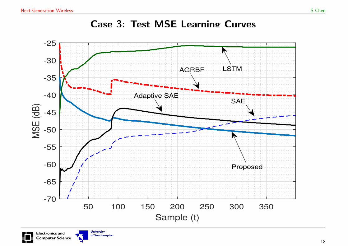
Case 3: Test MSE Learning Curves

50 100 150 200 250 300 350

Sample (t)

-70

-65

-60

-55

-50

-45

-40

-35

-30

-25M

SE

(dB

)

LSTM

Adaptive SAE

AGRBF

Proposed

SAE

18


Conclusions

• Deep neural networks, such as stacked autoencoder, has deep nonlinear learningcapability, but it is impossible to adapt network structure online in real time

• Shallow gradient RBF network has excellent adaptability

• We have shown how to integrate deep nonlinear learning capability of SAE withexcellent adaptability of adaptive GRBF

• Proposed deep neural network architecture is capable of adapting to changingunderlying system dynamics in real-time

– Particularly suitable for online modeling of highly nonlinear and nonstationaryindustrial processes

19

towards fully adaptive deep neural networks

Documents