towards infield, live plant phenotyping using a … › content › pdf › 10.1007 ›...
TRANSCRIPT

Machine Vision and Applications (2020) 31:2https://doi.org/10.1007/s00138-019-01051-7
ORIG INAL PAPER
Towards infield, live plant phenotyping using a reduced-parameterCNN
John Atanbori1 · Andrew P. French1,2 · Tony P. Pridmore1
Received: 2 October 2018 / Revised: 11 April 2019 / Accepted: 6 November 2019 / Published online: 17 December 2019© The Author(s) 2019
AbstractThere is an increase in consumption of agricultural produce as a result of the rapidly growing human population, particularlyin developing nations. This has triggered high-quality plant phenotyping research to help with the breeding of high-yieldingplants that can adapt to our continuously changing climate. Novel, low-cost, fully automated plant phenotyping systems,capable of infield deployment, are required to help identify quantitative plant phenotypes. The identification of quantitativeplant phenotypes is a key challenge which relies heavily on the precise segmentation of plant images. Recently, the plantphenotyping community has started to use very deep convolutional neural networks (CNNs) to help tackle this fundamentalproblem. However, these very deep CNNs rely on somemillions of model parameters and generate very large weight matrices,thus making them difficult to deploy infield on low-cost, resource-limited devices. We explore how to compress existing verydeep CNNs for plant image segmentation, thus making them easily deployable infield and on mobile devices. In particular,we focus on applying these models to the pixel-wise segmentation of plants into multiple classes including background,a challenging problem in the plant phenotyping community. We combined two approaches (separable convolutions andSVD) to reduce model parameter numbers and weight matrices of these very deep CNN-based models. Using our combinedmethod (separable convolution and SVD) reduced the weight matrix by up to 95% without affecting pixel-wise accuracy.These methods have been evaluated on two public plant datasets and one non-plant dataset to illustrate generality. We havesuccessfully tested our models on a mobile device.
Keywords Pixel-wise segmentation for plant phenotyping · Lightweight deep convolutional neural networks ·Separable convolutions · Singular value decomposition
1 Introduction
The world population will reach 9.1 billion by 2050, about34% higher than it is today. The UN Food and Agricul-ture Organisation (FAO) has estimated that in order to feedthis larger and more urban population, food production mustincrease by 70% [5]. Plant phenotyping will play an impor-
B John [email protected]
Andrew P. [email protected]
Tony P. [email protected]
1 School of Computer Science, University of Nottingham,Nottingham NG8 1BB, UK
2 School of Biosciences, University of Nottingham,Nottingham LE12 5RD, UK
tant role in achieving this target. Plant phenotyping refers toa quantitative description of the plant’s anatomical, physio-logical and biochemical properties [34]. Traditionally, plantphenotyping is carried out by experts and involves manuallymeasuring and recording plant traits, such as plant size andshape, number of leaves and flowers. High-quality, precisephenotyping of various plant traits can help improve yieldunder different climatic conditions (Fig. 1).
However, recently, image-based plant phenotyping hasgained more attention due to its inherent merits in handlinglarge-scale phenotyping: it is less tedious and error prone. Inparticular, image-based phenotyping techniques have beenused in plant segmentation [1,3] and leaf counting [1,3,11]and to automatically identify root and leaf tips [24]. Mostof these approaches rely on visual plant trait identification,before measuring quantities that provide the data to discoverhigh-yielding crops under different climatic conditions.
123

2 Page 2 of 14 J. Atanbori et al.
Fig. 1 Flower and leaf images in the first row, their ground truthmask inthe second row and the predicted CNN mask in the last row. The plantsand flowers classes are predictedwith a different colour indicating class.Images sources: The plant phenotyping and Oxford Flower datasets
Today, deep convolutional neural networks have beenused to phenotype plants in an attempt to gain much betteraccuracy [1,21,22,25,28]. In the computer vision commu-nity, these models have been shown to increase accuracybut at the expense of very many parameters (in millions)and expensive computations in the convolution layers (moremultiplications and additions) [7,17,19,39,42]. Due to thenumber of model parameters, they are sometimes inefficienton low-cost, resource-limited devices.
Jin et al. [15], Wang et al. [35] and Iandola et al. [14] haveattempted to reduce the computation time of CNNs, but themethods used by themwere not applied to plant phenotyping.Theobjective of this research is to demonstrate howverydeepCNNmodel parameters can drastically be reduced in numberwith very little reduction in pixel accuracy. In this paper wepresent the following new contributions. We have:
1. Formed ‘tiny’models (modelswith the number of param-eters drastically reduced) for pixel-wise segmentationby reducing the parameters of baseline very deep con-volutional neural networks using separable convolution,without compromising pixel accuracy.
2. Demonstrated that the accuracy of these tiny models wasas good as their baseline counterparts (un-compressed)on plant phenotyping datasets and a non-plant dataset.
3. Formed very tiny models (smaller weight matrix thanthe tiny models) using SVD and demonstrated on plantphenotyping datasets and a non-plant dataset that theirpixel accuracy remains practically unaffected.
4. Evaluated the size of our ‘tiny’ models’ parameters withexisting popular CNNs, demonstrating their potential forinfield deployment.
The remainder of this paper is structured as follows.In Sect. 2, we review existing work that reduces modelparameters and/or the weight matrix for devices with lim-
ited resources. In Sect. 3, we introduce the two public plantphenotyping datasets and the non-plant dataset used in ourexperiments and proceed in Sect. 4 to describe our meth-ods used in compressing the baseline CNNs designed forpixel-wise segmentation. We describe our experimental set-up including a benchmark in Sect. 5. Then we proceed topresent and discuss our results in Sect. 6 and conclude inSect. 7
2 Related work
Traditionally, plant phenotyping approaches using computervision have looked at plant density estimation from RGBimages [16,18,30] and counting leaves using a simple arti-ficial neural network (ANN) or a support vector machine(SVM). However, these approaches are sometimes not fullyautomated and require some feature selection techniques tobe applied prior to training classifiers. Minervini et al. [21]extracted dense SIFT descriptors from the green colour chan-nel and quantised the SIFT space using k-means clusteringto create a codebook for segmentation of plants. In a colla-tion study [28], segmenting and counting leaves have alsoused traditional computer vision methods. The best resultsfrom these were based on super-pixel-based methods, water-sheds and Chamfer matching. The results of these methodsdepend on the user fine-tuning parameters of the system andtherefore may make them difficult for infield use. The super-pixel-based method needs the fine-tuning of five parameters,including those of canny edge detector in order to achievegood results. The watershed approach requires the use ofmorphological operations after plant segmentation to removenoise in the segmentation. This not only adds a step to theprocess but also requires additional parameter tuning step bythe user.
More recent computer vision approaches to plant pheno-typing are based on deep learning methods; these have beenshown to perform better than the traditional methods [1].Aich and Stavness [1] adopted the SegNet architecture andachieved better results on the dataset used in [21,28]. Themethods used by Aich and Stavness [1] have been used suc-cessfully by Aich et al. [3] in estimating phenotypic traitsfrom wheat images and also in conjunction with global sumpooling [2] for counting wheat spikes accurately. Anotherplant phenotyping approach that uses deep learning achievedstate-of-the-art automatic identification of ear base, leaf base,root tips, ear tips and leaf tips inwheat [24]. These deep learn-ing approaches for plant phenotyping have beenmotivated bythe recent successes in applying them to other fields for bothsegmenting and classification, some of which are consideredin the remaining paragraphs of this section.
Long et al. [19] have popularised CNNs for dense pre-dictions. The key features of their work are the 1 × 1
123

Towards infield, live plant phenotyping using a reduced-parameter CNN Page 3 of 14 2
convolution with the channel dimension equal to the num-ber of classes being predicted, and a deconvolution layerused for bilinear up-sampling of the coarse outputs to adense pixel output for prediction. Badrinarayanan et al. [7],however, showed that using the max-pooling indices toup-sample the coarse outputs can increase the pixel accu-racy of the model. While Badrinarayanan et al. reportedsome improvements in pixel accuracies over the methodsused by Long et al., their decoder had more parametersand was therefore less memory efficient. There have beenother semantic segmentation networks [17,40,42], whichachieved better pixel accuracies on similar datasets. How-ever, these networks are very deep and thus have moreparameters and use up more memory. The shortcomingsof most convolutional neural networks lie within the con-volutional layers and the fully connected layers. In theconvolutional layer, the multiply and add operations aretime-consuming and the fully connected layers also gen-erate many parameters. It has been demonstrated by Yuet al. [38] that even though recognition accuracies ofdeep neural networks improve as the depth of a networkincreases, a large proportion of the parameters generatedby these models contribute little to recognition and pixelaccuracy.
Various attempts to reduce network size have focused onthinning the convolutional layer, reducing parameters in thefully connected layer of networks and compressing weightmatrices generated by network models. While the first twofocus on speeding up the training of models, the last focuseson testing. Reducing the number of parameters in a networkcan be achieved using a 1× 1 convolution after 3× 3 convo-lutions as in Inception [33] and ShuffleNet [41]. Depthwiseseparable convolutions have also been used in MobileNet[13] and Xception [8] to achieve this. ShuffleNet [41], how-ever, used a combination of the two approaches. Since thevast majority of weight parameters reside in the fully con-nected layers, truncated SVD has been used in [9,10,31,37]to reduce weight matrices in these layers. Denton et al. [9]and Girshick [10] demonstrated that using SVD speed upprediction while keeping accuracy within 1% of the originalmodel.
The traditional approaches to plant phenotyping are usu-ally semi-automated and thus not suitable for infield applica-tion. Recent developments in image-based plant phenotypingare based on state-of-the-art CNN methods. Even thoughthese methods can be fully automated, they require signif-icant storage and memory, thus making them unsuitablefor deployment on low-cost devices (especially those withlimited memory and processing power). Some current devel-opments in CNNs aim to reduce their number of parameters,thusmaking themmore efficient on low-cost devices but withsome reduction in accuracy. This work, which builds on ourprevious [6], is based on this premise and, to the best of our
Fig. 2 The Oxford flower dataset
knowledge, is one of the first applied to infield plant pheno-typing.
Similar to our work, previous authors [4] have attemptedto reduce theFCNandSegNetmodel parameters by replacingthe deconvolution operationwith sub-pixels [29]which intro-duced a negligible computational cost. However, our work isdifferent from sub-pixel convolution since we focused onreducing parameters by replacing two-dimensional convolu-tions with two-dimensional separable convolution and thenapplying SVD.
3 Datasets
We use two plant datasets: the Oxford flower dataset (Fig.2) [23] and the CVPPP leaf segmentation challenge datasetalso known as the plant phenotyping dataset (Fig. 3) [20,21]and a non-plant dataset, the CamVid dataset (Fig. 4) [7] toperform our experiments.
The Oxford flower dataset has ground truth segmenta-tion for most images. We use the same criteria as Nilsbackand Zisserman [23] to form our segmentation dataset: flowerclasses that were under-sampled in the original dataset wereremoved. Following these criteria, five classes (DandelionTaraxacum, lily of the valley Convallaria majalis, CowslipPrimula veris, Tulip Tulipa and BluebellHyacinthoides non-scripta) had insufficient images and were removed. Thisleaves 12 flower classes with a total of 753 images. Examplesof images in this dataset are shown in Fig. 2.
The plant phenotyping dataset is a challenging datasetintroduced in [21] and available online at http://www.plant-phenotyping.org/datasets.Weused all 165Arabidopsisimages (Arabidosis thaliana) in the Ara2013 dataset and 62
123

2 Page 4 of 14 J. Atanbori et al.
Fig. 3 The plant phenotyping dataset
Fig. 4 The CamVid dataset
tobacco (Nicotiana tabacum) images in the datasets. Exam-ples of images in this dataset are shown in Fig. 3.
The CamVid dataset is a road scene understanding datasetwith 367 training images, 101 validation images and 233 test-ing images of day and dusk scenes, available at http://mi.eng.cam.ac.uk/research/projects/VideoRec/CamVid/. The chal-lenge is to segment 12 classes, including background, suchas road, building, cars, pedestrians, signs, poles, and side-walk. Examples of images in this dataset are shown inFig. 4.
All plant datasets were first divided into ‘80/20’ fortrain/test; then the training data were further divided into‘80/20’ for training/validation. We normalise all images byscaling RGB values to the range 0–1, before passing them tothe deep neural networks. The RGB image annotations werefirst converted into a class label. For example, an RGB value
of [255, 255, 0] belonging to class one is represented as [1,1, 1], RGB value [255, 64, 64] belonging to class two is rep-resented as [2,2,2], and so on. Finally, we converted the classlabels into a binary class matrix (one-hot encoding) beforepassing them to our networks.
4 Methods
Wehave reducedmodel parameters of three popular semanticsegmentation networks (FCN, SegNet and Sub-Pixel) usingthe two methods detailed in this section. We used separableconvolutions to reduce the model parameter number beforetraining the network, and singular value decomposition toreduce weight matrix size after.
4.1 Separable convolution
MobileNet [13], MobileNetV2 [27] and Xception [8] useseparable convolution to reduce the model parameters. Sepa-rable convolution reduces the number of multiplications andadditions in the convolutional operation, thus reducing themodel’s weight matrix and speeding up the training and test-ing of large CNNs.
A 2D convolution can be defined as in Eq. 1.
y(m, n) =k−1∑
i=0
k−1∑
j=0
h(i, j)x(m − i, n − j) (1)
where x is the (m×n)matrix being convolved with a (k×k)kernel h. If the kernel h can be separated into two kernels, sayh1 of dimension (m × 1) and h2 of dimension (1 × n), thenthe 2D convolution can be expressed as a 1D convolution asin Eq. 2.
y(m, n) =k−1∑
i=0
h1(i)
[ k−1∑
j=0
h2( j)x(m − i, n − j)
](2)
The 2D convolution requires k × k multiplications andadditions. However, in the case of separable convolution,since the kernel is decomposed into two 1D kernels, therequired multiplications and additions are reduced to k + k,thus reducing the number of model parameters.
We converted the 2D convolutions in the baseline seman-tic segmentation networks (FCN, SegNet and Sub-Pixel)into separable versions. For SegNet, the convolutional lay-ers in both the encoder and decoders were made separable.However, with FCN and Sub-Pixel only the encoders wereseparable, as the decoder had few or no parameters. Wethen applied batch normalisation and ReLU activations tothe separable convolutions. It is important to note that thefirst convolution layer of each network was not separated, as
123

Towards infield, live plant phenotyping using a reduced-parameter CNN Page 5 of 14 2
Fig. 5 Architecture of our Tiny-FCN. This is a typical VGG-19 archi-tecturewith only four blocks. The building blocks are comprised of a 2Dconvolution (Conv2D), 2D seperable convolution (SeparableConv2D),batch normalisation (BN), a ReLU activation, max-pooling and up-sampling
Fig. 6 Architecture of ourTiny-SegNet. This is a typicalVGG-19 archi-tecturewith only four blocks. The building blocks are comprised of a 2Dconvolution (Conv2D), 2D seperable convolution (SeparableConv2D),batch normalisation (BN), ReLU and softmax activations, max-poolingand up-sampling
this holds important high-detail features. The reduced archi-tectures are illustrated in Figs. 5 and 6
4.2 Singular value decomposition
Singular value decomposition, which has been successfullyapplied to image compression [26], can be used to reducethe size of weight matrices [9,10,37]. AssumingW ∈ R
m×n
is the weight matrix from the separable convolutions model,then the singular value decomposition of matrix W can befactorised into the form shown in Eq. 3.
W = U · S · V T (3)
where U ∈ Rm×n is an m × n left-singular vector, V ∈
Rn×n is an n × n right-singular vector and S ∈ R
n×n is ann × n rectangular diagonal matrix called the singular valuesof the weight matrix W . Then assuming diagonals of S ={d(1,1), d(2,2), d(3,3)..., d(n,n)} and {d(1,1) ≥ d(2,2) ≥ d(3,3) ≥... ≥ d(n,n) ≥ 0}, we can reconstruct a new matrix W ′ as inEq. 4
W ′ = U ′ · S′ · V T ′(4)
where U′ ∈ Rm×k , VT′ ∈ R
k×n and S′ ∈ Rk×k .
W′ ∈ Rm×n is the reconstructed weight matrix, which has
the same dimensions as W . It is important to note that W ′was reconstructed with the first k singular values of S andk = min(m, n). Selecting k in this way reduces the size ofthe weight matrix.
We compressed the weight matrices generated by the sep-arable convolution models (which we call Tiny-FCN, Tiny-SegNet andTiny-Sub-Pixel) to formavery tinymodel (whichwe call Very-Tiny-FCN, Very-Tiny-SegNet and Very-Tiny-Sub-Pixel, respectively) using the SVD approach presentedin this section. In both models, we skipped the first threeblocks and only applied SVD to the remainder, as this willensure that high-detail features are not lost and thus not drasti-cally reduce themodel’s performance, as the first three blocksalready have a small number of parameters.
5 Experiments
For our evaluation, we used the three datasets detailed inSect. 3 to perform the following experiments. We produce:
– Pixel-wise segmentation into classes using the originalsemantic segmentation networks (FCN, SegNet and Sub-Pixel)
– Pixel-wise segmentation into classes using our tiny mod-els, Tiny-FCN, Tiny-SegNet and Tiny-Sub-Pixel, whichis made up of only separable convolutions.
– Pixel-wise segmentation into classes using our very tinymodels, Very-Tiny-FCN, Very-Tiny-SegNet and Very-Tiny-Sub-Pixel, which is made up of separable convo-lutions and SVD.
– Background and foreground segmentation (two classes)of the Oxford flower dataset to help further evaluate themodels on smaller datasets and to show that the baselinemodels performed better with fewer classes.
5.1 Set-up
We perform all our experiments using the VGG-16 stylearchitecture but without the last block, known as VGG-16Basic, as recommended by Badrinarayanan et al. [7] when
123

2 Page 6 of 14 J. Atanbori et al.
evaluating SegNet, FCN and Sub-Pixel. The convolutionallayers in each model’s encoder were followed by batch nor-malisation and ReLU activation layers. Except for the last,we placed a max-pooling layer at the end of each encoderblock.
The FCN architectures (including the ‘Tiny’ versions)used the FCN-8 decoder style as described in [19]. Since theFCN’s decoder had fewer parameters, we did not performseparable convolutions on them. However, with the excep-tion of the first layer, all convolutional layers of theTiny-FCNencoder were converted into separable convolutions and theneachwas followedby a batch normalisation andReLUactiva-tion layers. The set-up of the Sub-Pixel architecture is similarto the FCN but its decoder is made of sub-pixel convolution,which generates no parameters.
The SegNet used same settings as in [7] and we usedthe max-pooling indices for up-sampling. Tiny-SegNet’sencoder used a similar set-up as the Tiny-FCNs. Similarly,apart from the first layers, all convolutional layers were con-verted into a separable convolution and followedwith a batchnormalisation andReLUactivation layers.UnlikeTiny-FCN,we applied separable convolutions to all convolutional layersof SegNet decoder and followed themby batch normalisationand ReLU activation layers, to form our Tiny-SegNet model.
Training of the CNN models was performed on a Linuxserver with three GeForce GTX TITAN X GPUs (12 GBmemory each). The models were implemented using Python3.5.3 and Keras 2.0.6 with Tensorflow backend and weretested on a windows 10 computer with 64 GB RAM and a3.6 GHz processor. We also developed a mobile app to testcapabilities of our tiny models using Android studio 3.1.2 onwindows and tested it using a 1) Samsung Galaxy J1 mobilephone running Android 4.4 and 2) Google Nexus 5x mobilephone emulator running Android 8.1.
5.2 Benchmarks
For benchmarking, we compared with the baseline mod-els (FCN, SegNet and Sub-Pixel) on the three datasets, theOxford flower dataset (http://www.robots.ox.ac.uk/~vgg/data/flowers/17/index.html), the plant phenotyping data-set (http://www.plant-phenotyping.org/datasets) and theCamVid dataset (http://mi.eng.cam.ac.uk/research/projects/VideoRec/CamVid/), We compare the results to our ‘tiny’models (Tiny-FCN, Very-Tiny-FCN, Tiny-SegNet and Very-Tiny-SegNet). In particular, we evaluated the following:
– Number of parameters per our model versus the baselinedeep CNN models.
– Size of weight matrix per our model versus the baselinedeep CNN models
– Accuracy (pixel accuracy, mean IoU, precision andrecall) per model
– Average processing time using three devices for segmen-tation.
We also performed background and foreground (two-class) segmentation with the Oxford flower dataset to eval-uate the performance of the FCN, SegNet and Sub-Pixelmodels with the multi-class segmentation. We tested the tinymodels on two types of mobile device: Google Nexus 5xand Samsung Galaxy J1 smartphone. The Samsung GalaxyJ1 was used also for real-time infield segmentation, to showthat the tiny models work on mobile devices infield. Finally,we compare tiny and very-tiny model parameters to somepopular existing models (see Table 8) that have used someform of parameter and or weight matrix reduction technique.
For all models, we set the number of epochs to 200 with abatch size of 6. We use categorical cross-entropy loss as theobjective function for training the network and anAdamopti-miser with an initial learning rate of 0.001. We then reducedthe learning rate by a factor of 10 whenever training plateausfor more than 10 epochs. The input images were all resizedto (224× 224) since most input images were approximatelythis size, and also to help avoid a fractional output size thatmay result from the max-poolings in the network. We didnot apply data augmentation as there were no problems ofoverfitting and the performance of the models was good.
Due to the large variations in the number of pixels in eachclass as per the training samples, we weighted the loss dif-ferently based on the true class (known as class balancing).We applied median frequency balancing, which is the ratioof median class frequency computed on the entire trainingsamples divided by the class frequency. The implication ofthis is that larger classes in the training set are given lessweight, while smaller ones are given more.
Fig. 7 The training and validation loss versus epochs’ curves for theflower dataset based on the SegNet model
123

Towards infield, live plant phenotyping using a reduced-parameter CNN Page 7 of 14 2
Fig. 8 The training and validation loss versus epochs curves for theflower dataset based on the Tiny-Sub-Pixel model
Finally, we ensured that the baselinemodels and tinymod-els neither over- nor underfit by monitoring the training andvalidation losses. Figures 7 and 8 show the loss curves forSegNet and Tiny-Sub-Pixel on the flower dataset for 200epochs. Both figures represent a drop in training and valida-tion error as the number of epochs increases, which indicatesthat the networks are learning from the data that are givenas input and not overfitting or underfitting. Similar patterncurves occurred for all the other models, which can be down-loaded from this section’s footnote 1.
5.3 Metrics used
We report four metrics from common pixel-wise segmen-tation evaluations that are variations on pixel accuracy andregion intersection over union (IoU), where ni j is the numberof pixels of class i predicted to belong to class j , n ji is thenumber of pixels of class j predicted to belong to class i andc is the total number of classes.
– Pixel accuracy: This tells us about the overall effective-ness of the classifier and is defined in Eq. 5.
∑ci=1 nii∑c
i=1(∑c
j=1 ni j )(5)
– Mean IoU: This compares the similarity and diversity ofthe complete sample set and is defined in Eq. 6:
1
c∗
c∑
i=1
nii∑cj=1 ni j + (
∑cj=1 n ji ) − nii
(6)
1 https://github.com/Amotica/Low-Cost-Plant-Phenotyping.
– Average Precision: This tells us about the class agree-ment of the data labels with the positive labels given bythe classifier and is defined in Eq. 7.
1
c∗
c∑
i=1
nii∑cj=1 n ji
(7)
– Average Recall: This is the effectiveness of classifier toidentify positive labels and is defined in Eq. 8.
1
c∗
c∑
i=1
nii∑cj=1 ni j
(8)
6 Results
Table 1 shows the results of parameter reduction whenwe applied only separable convolutions (Tiny-FCN, Tiny-SegNet and Tiny-Sub-Pixel models) and when we com-bined separable convolutions and SVD (our Very-Tiny-FCN,Very-Tiny-SegNet and Very-Tiny-Sub-Pixel models). Thehighlighted rows show data for the existing pixel-wise seg-mentation models, which we used as our baseline models.
The models compressed with only separable convolu-tion achieved a little above 88% in storage space savings.However, our models compressed using both separable con-volution and SVD had the most storage space savings.
Table 2 shows the accuracies of the baseline deep CNNmodels versus their tiny counterparts. These results are basedon segmenting the test samples of the plant phenotypingdataset into three classes (background, Tobacco (Nicotianatabacum) and Arabidopsis (Arabidopsis thaliana) plants).The best performing models based on this dataset are theFCNs and Sub-Pixel, which outperformed the SegNet mod-els by almost 1% based onmean IoU. The difference in meanIoU between the tiny models and original deep CNN coun-terpart is less than 0.75% and 0.02% for the SegNet andFCN, respectively, which shows that our compressed FCNandSegNetmodels are comparable to the original deepCNN.
In Table 3, we present the accuracies of the baseline deepCNN models versus their tiny counterparts on the test sam-ples in the Oxford flower dataset, segmenting into 13 classesincluding the background. The results show the SegNet mod-els to perform better than the FCN based on all the evaluationmetrics. The baseline SegNet and FCNmodels outperformedtheir tiny counterparts by less than 0.01% and 0.35% basedon mean IoU, respectively. This shows the tiny models to becomparable to the baselines used in our experiments.
To further investigate the results and illustrate generalityof our multi-class segmentation, we trained all models onthe CamVid dataset, which is of similar size as our multi-class flower dataset but for a different problem domain (road
123

2 Page 8 of 14 J. Atanbori et al.
Table 1 Model parameters andsize of weight matrices on discfor all models used in ourexperiments
Parameters Weight matrix
# Reduction (%) Size on disc (MB) Storage savings (%)
FCN 7,647,950 – 87.6 –
Tiny-FCN 885,528 88.42 10.2 88.36
Very-Tiny-FCN 885,528 88.42 3.51 95.99
SegNet 17,649,795 – 202.0 –
Tiny-SegNet 2,034,499 88.47 23.4 88.42
Very-Tiny-SegNet 2,034,499 88.47 7.96 96.06
Sub-Pixel 7,646,043 – 88.0 –
Tiny-Sub-Pixel 881,142 88.48 10.9 87.6
Very-Tiny-Sub-Pixel 881,142 88.48 3.6 95.9
The baseline models have been highlighted in bold
Table 2 Accuracies for bothoriginal and tiny models basedon the plant phenotyping dataset
Precision (%) Recall (%) Pixel accuracy (%) Mean IoU (%)
FCN 98.59 98.57 98.58 95.49
Tiny-FCN 98.45 98.44 98.45 95.47
Very-Tiny-FCN 98.45 98.44 98.45 95.47
SegNet 98.27 98.20 98.23 94.82
Tiny-SegNet 98.09 98.03 98.06 94.07
Very-Tiny-SegNet 98.09 98.03 98.06 94.07
Sub-Pixel 98.68 98.62 98.65 96.20
Tiny-Sub-Pixel 98.73 98.56 98.65 96.18
Very-Tiny-Sub-Pixel 98.73 98.56 98.65 96.18
Plants were segmented into three classes
Table 3 Accuracies for bothoriginal and tiny models basedon the Oxford flower dataset
Precision (%) Recall (%) Pixel accuracy (%) Mean IoU (%)
FCN 94.98 94.02 94.38 72.73
Tiny-FCN 94.08 93.29 93.57 72.38
Very-Tiny-FCN 94.08 93.29 93.57 72.38
SegNet 95.08 94.26 94.41 74.51
Tiny-SegNet 94.46 94.06 94.20 74.50
Very-Tiny-SegNet 94.46 94.06 94.20 74.50
Sub-Pixel 94.21 94.04 94.04 72.18
Tiny-Sub-Pixel 93.81 93.60 93.72 71.92
Very-Tiny-Sub-Pixel 93.81 93.60 93.72 71.92
The flowers were segmented into 13 classes
scenes instead of plants). Table 4 shows the accuracies ofbaseline deep CNN models versus their tiny counterpartsbased on segmenting test samples of this dataset into 12classes including the background. We observe an interestingresult, which this time shows the FCN models to outper-form the SegNet models by approximately 1%. Furthermore,the very deep FCN and SegNet models outperformed theirtiny counterparts by approximately 3% and 0.8% mean IoU,respectively.
We segmented the test samples in the Oxford flowerdataset into just two classes (background and flower) using
all baseline and tiny models. We present the results in Table5. The result shows the baseline deep CNNmodels, and theirtiny counterparts, to perform better on this dataset with twoclasses. The two-class problem outperformed the 13-classproblem by approximately 19% based on mean IOU alone.SegNet outperformed FCN on this problem domain by a verynarrow margin. Furthermore, even though SegNet was thebest performing model, the other models remain compara-ble.
Finally, we developed mobile applications using Androidstudio to show that our tiny models can run well on these
123

Towards infield, live plant phenotyping using a reduced-parameter CNN Page 9 of 14 2
Table 4 Accuracies for bothoriginal and tiny models basedon the CamVid dataset
Precision (%) Recall (%) Pixel accuracy (%) Mean IoU (%)
FCN 93.01 92.73 92.25 55.89
Tiny-FCN 90.73 88.88 88.98 51.59
Very-Tiny-FCN 90.73 88.88 88.98 51.59
SegNet 92.59 89.75 90.85 54.48
Tiny-SegNet 90.87 89.77 89.80 53.69
Very-Tiny-SegNet 90.87 89.77 89.80 53.69
Sub-Pixel 93.51 88.72 88.85 51.89
Tiny-Sub-Pixel 90.53 88.12 88.28 51.77
Very-Tiny-Sub-Pixel 90.53 88.12 88.28 51.77
The road scenes were segmented into 12 classes (including the background)
Table 5 Accuracies for bothoriginal and tiny models basedon the Oxford 17 flower dataset
Precision (%) Recall (%) Pixel accuracy (%) Mean IoU (%)
FCN 97.10 97.10 97.10 93.29
Tiny-FCN 96.80 96.80 96.80 92.64
Very-Tiny-FCN 96.80 96.80 96.80 92.64
SegNet 97.27 97.27 97.27 93.65
Tiny-SegNet 97.08 97.08 97.08 93.24
Very-Tiny-SegNet 97.08 97.08 97.08 93.24
Sub-Pixel 97.18 97.18 97.18 93.47
Sub-Pixel 96.92 96.92 96.92 92.87
Tiny-Sub-Pixel 96.92 96.92 96.92 92.87
The flowers were segmented into two classes (flowers and background)
devices compared with the baseline models. We tested theapplications on a Google Nexus 5X emulator and SamsungGalaxy J1 smartphone. Figures 9 and 10 show the results ofsegmentation on the flowers dataset for Google Nexus 5Xand Samsung Galaxy J1, respectively. We have also includedFig. 11, which shows the results of using the SamsungGalaxy J1 for segmenting leaf images collected from theinternet. The Samsung Galaxy J1 has been used infield suc-cessfully to segment flowers,while theGoogleNexus 5Xwasonly emulated with Android studio. The average processingspeed was tested for segmenting flowers and leaves only. Weused the data captured infield with the Samsung Galaxy J1to test the flower mobile application, and a set of images col-lected from the web to test the leaf mobile application, andthen discuss these results in Sect. 6.1.
We noted that the smaller parameter models were fasterin segmenting both flowers and leaves (see Tables 6 and 7).As expected, the ‘tiny’ models process faster than the base-line model since they have fewer parameters. The FCN andSub-Pixel-based models with only 0.9 million parameterssegment flowers and leaves nearly 2 s faster than the SegNetmodels for 13 classes (see Table 7).
The average processing speed of segmenting a singleflower infield with the Samsung J1 mobile phone is 3.32and 3.95 s for the two- and 13-class problems, respectively.
Fig. 9 Mobile test results using Google Nexus 5X emulators. Fromleft to right: Flower segmentation into 13 classes, leaf segmentationinto 3 classes and flowers segmentation into 2 classes (foreground andbackground)
Segmenting the same images using aWindows computer or aGoogle Nexus 5xmobile phone emulator is faster due to theirconsiderably higher processing power. Considering that theSamsung J1 only runs anAndroid 4.4.4 compared toAndroid8.1 on Google Nexus 8.1 further justifies the results.
Both baseline FCN and Sub-Pixelmodels have 7.6millionparameters and take approximately 3 s to segment a floweror a leaf on a windows 10 computer, 5 s on the Google Nexus
123

2 Page 10 of 14 J. Atanbori et al.
Fig. 10 Real-time infield test on Samsung Galaxy J1 smart phone. Thiswas performed only for the flowers dataset
Fig. 11 Segmenting leaf data collected from the internet on the Sam-sung Galaxy J1 smart phone
Table 6 Average processing speed in seconds for segmenting a leaf anda flower into two or 13 classes using the tiny models
Windows Nexus 5x Samsung J1
Tiny-FCN
Flower-2 classes 0.10 ± 0.01 0.18 ± 0.03 3.32 ± 0.24
Flower-13 classes 0.11 ± 0.02 0.19 ± 0.03 3.95 ± 0.30
Leaf 0.12 ± 0.02 0.20 ± 0.05 3.91 ± 0.14
Tiny-SegNet
Flower-2 classes 0.16 ± 0.02 0.21 ± 0.03 5.32 ± 0.14
Flower-13 classes 0.18 ± 0.01 0.27 ± 0.06 6.13 ± 0.23
Leaf 0.17 ± 0.07 0.31 ± 0.07 6.42 ± 0.13
Tiny-Sub-Pixel
Flower-2 classes 0.13 ± 0.04 0.18 ± 0.05 3.92 ± 0.31
Flower-13 classes 0.14 ± 0.06 0.18 ± 0.04 4.21 ± 0.40
Leaf 0.14 ± 0.04 0.19 ± 0.07 4.37 ± 0.22
These have been tested on three devices (Windows 10 computer, GoogleNexus 5x emulator and Samsung J1 mobile). These were computedusing 15 test flower and leaf images. The average processing speedshows plus/minus standard deviation
5x and 23 s on the Samsung J1 mobile phone. The baselineSegNet model is the slowest to process a flower or leaf, eventhough this takes approximately 7 and 8 s on windows 10 andGoogle Nexus 5x, respectively. When segmenting with Seg-Net model (17.5 million parameters), the application crashes
Table 7 Average Processing speed in seconds for segmenting a leafand a flower into two or 13 classes using the Baseline models
Windows Nexus 5x Samsung J1
FCN
Flower-2 classes 2.59 ± 0.14 4.02 ± 0.17 22.41 ± 0.82
Flower-13 classes 2.73 ± 0.12 4.10 ± 0.10 23.05 ± 0.58
Leaf 2.37 ± 0.07 3.91 ± 0.12 22.90 ± 0.52
SegNet
Flower-2 classes 6.73 ± 0.14 7.95 ± 0.23 –
Flower-13 classes 6.93 ± 0.21 8.01 ± 0.15 –
Leaf 6.64 ± 0.16 7.75 ± 0.24 –
Sub-Pixel
Flower-2 classes 2.49 ± 0.10 3.96 ± 0.08 21.21 ± 059
Flower-13 classes 2.94 ± 0.13 4.03 ± 0.11 22.01 ± 071
Leaf 2.91 ± 0.09 3.89 ± 0.11 21.73 ± 0.61
These have been tested on three devices (Windows 10 computer, GoogleNexus 5x emulator and Samsung J1 mobile). These were computedusing 15 test flower and leaf images. The average processing speedshows plus/minus standard deviation
due to the large number of parameters and the low processingpower of this device.
6.1 Discussion
We present in Table 8 the number of parameters in millionsfor some popular segmentationmodels. The topmodels wereour Tiny-FCN, Very-Tiny-FCN, Tiny-Sub-Pixel and Very-Tiny-Sub-Pixel models, which all had less than a millionparameters. The Very-Tiny-Sub-Pixel had the smallest num-ber of parameters when compared to the nearest thousand.The replacement of the decoders with sub-pixel convolutionmade this possible. The other models used some form ofparameter reduction techniques while preserving the accu-racy of the model. SqueezeNet (1.3 million) was the nextmodel reduced in parameters followed by our Tiny-SegNetand Very-Tiny-SegNet models and then MobileNet, whichwere all designed for mobile platforms.
Howard et al. [13] reported that reducing CNN modelparameters using separable convolution usually reduces theaccuracy of the network. The experiments we performedalso confirm this finding. We observed that with a care-ful reduction in the number of parameters in the baselinedeep CNN model, accuracies are comparable. We noted thatwhen using separable convolutions to reduce model param-eters, a good practice is not to apply them to convolutionallayers with a smaller number of parameters. For example,we only applied separable convolutions to the FCN encoderbut not the decoder. Due to this, Howard et al. had used aparameter called depth multiplier which controls the num-ber of channels generated as output (output_channels =
123

Towards infield, live plant phenotyping using a reduced-parameter CNN Page 11 of 14 2
Table 8 Comparing parameters of some popular models with ours
Model Parameters (Millions)
Tiny-FCN (Ours) 0.9
Very-Tiny-FCN (Ours) 0.9
Tiny-Sub-Pixel (Ours) 0.9
Very-Tiny-Sub-Pixel (Ours) 0.9
SqueezeNet [14] 1.3
Tiny-SegNet (Ours) 2.0
Very-Tiny-SegNet (Ours) 2.0
MobileNet[13] 4.2
GoogleNet [32] 6.8
Sub-Pixel [4] 7.6
FCN (VGG-16 Basic) [19] 7.6
VGG-16 Compressed [12] 11.3
AlexNet - QCNN [36] 12.6
SegNet (VGG-16 Basic)[7] 17.5
Xception [8] 22.9
Inception V3 [33] 23.2
SVD [9] 47.6
The number of parameters is in millions
input_channels∗depth_multiplier ). Thus, using a smallerdepth_multiplier shrinks the model parameters even fur-ther but at the expense of accuracy. We preferred to workwith a depth multiplier of one, as this produces good resultswhen separable convolutions are applied to large parametergenerating convolutional layers.
Furthermore, caution is needed when using singular valuedecomposition to reducemodelweightmatrices. Someworkshave reported a drop in accuracy when SVD is applied [9,10,31,37]. Our results show that applying SVD correctly furtherdecreases the size of weight matrices while preserving pixelaccuracies.
Skipping the first three convolutional layers, we applySVD (with k = 4) to all other convolutional layers to recon-struct the models’ weight matrices. This careful applicationof SVDnot only reduced the size of themodel on disc but alsoresulted in comparable pixel accuracies to the state-of-the-artnon-compressed counterparts.
Our tiny models’ performance on the plant phenotypingdatasets compare to their non-compressed counterparts. Ontest samples where the non-compressed models achievedgood segmentation results, the tiny models also did. Forexample, on the Oxford flower dataset (13-class problem),the Fritillary, Iris, Wind Flower, Colts’ Foot and Daisy testsamples in Fig. 13 were well segmented by all models. Addi-tionally, the non-compressed deepCNNcounterparts showedbetter results in some instances than the tiny models and viceversa (see examples in Fig. 14).
These observations are true for the plant phenotypingdataset too; see Fig. 12. Using the Oxford flower dataset
Fig. 12 Sample test instances from the Plant Phenotyping dataset
Fig. 13 Sample test instances from theOxford flower dataset with visu-ally very good segmentation (two classes)
Fig. 14 Multi-class segmentation: Sample test instances from theOxford flower dataset with some segmentation errors present
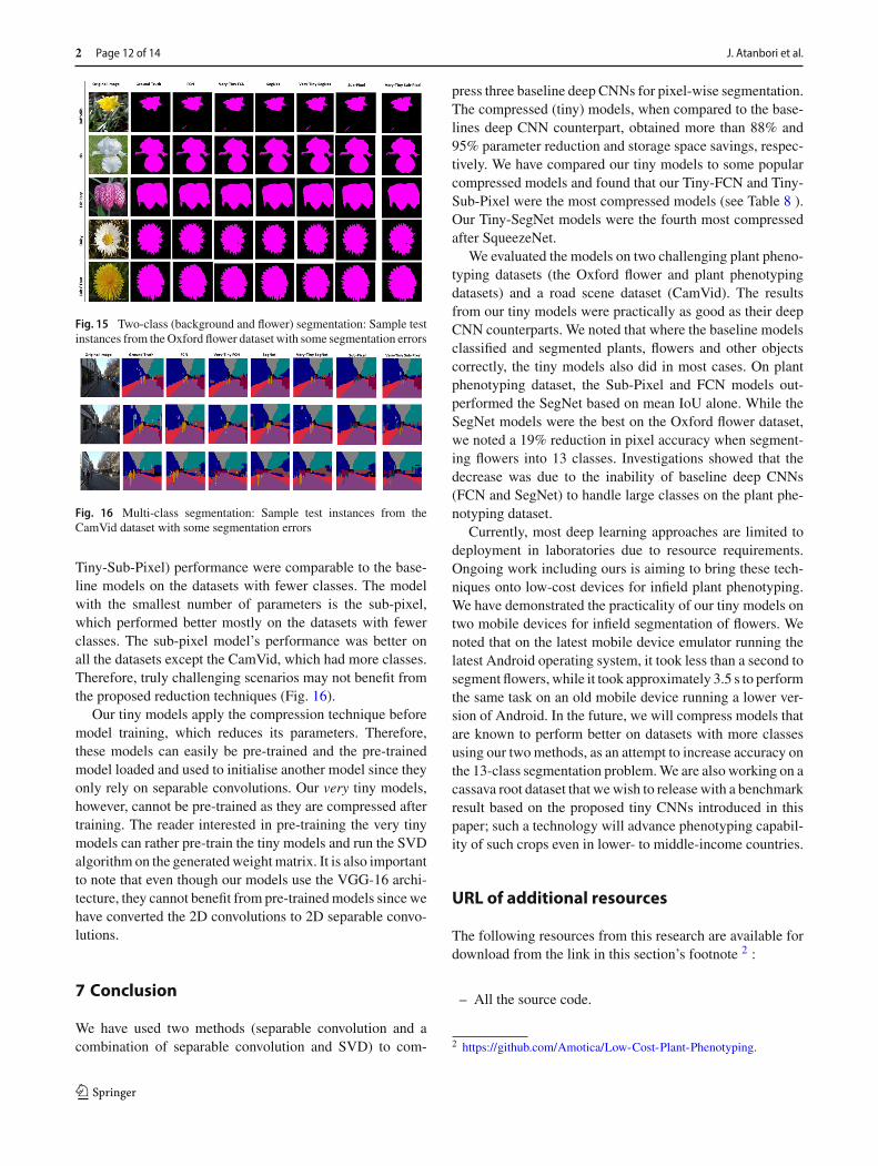
for background and foreground (flowers) segmentation, thesegmentation results of our tiny models were similar tothat of their non-compressed deep CNN counterparts (seeFig. 15).
The models with more parameters performed better onthe datasets with more classes. For example, SegNet with17.5 million parameters performed better on the flower andCamVid datasets when compared with all the other mod-els. However, the tiny models’ (Tiny-FCN, Tiny-SegNet and
123
2 Page 12 of 14 J. Atanbori et al.
Fig. 15 Two-class (background and flower) segmentation: Sample testinstances from theOxford flower dataset with some segmentation errors
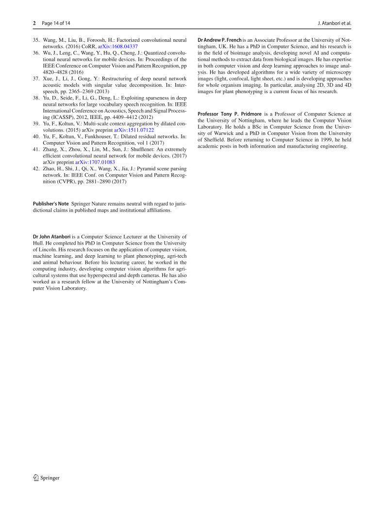
Fig. 16 Multi-class segmentation: Sample test instances from theCamVid dataset with some segmentation errors
Tiny-Sub-Pixel) performance were comparable to the base-line models on the datasets with fewer classes. The modelwith the smallest number of parameters is the sub-pixel,which performed better mostly on the datasets with fewerclasses. The sub-pixel model’s performance was better onall the datasets except the CamVid, which had more classes.Therefore, truly challenging scenarios may not benefit fromthe proposed reduction techniques (Fig. 16).
Our tiny models apply the compression technique beforemodel training, which reduces its parameters. Therefore,these models can easily be pre-trained and the pre-trainedmodel loaded and used to initialise another model since theyonly rely on separable convolutions. Our very tiny models,however, cannot be pre-trained as they are compressed aftertraining. The reader interested in pre-training the very tinymodels can rather pre-train the tiny models and run the SVDalgorithm on the generatedweightmatrix. It is also importantto note that even though our models use the VGG-16 archi-tecture, they cannot benefit from pre-trainedmodels since wehave converted the 2D convolutions to 2D separable convo-lutions.
7 Conclusion
We have used two methods (separable convolution and acombination of separable convolution and SVD) to com-
press three baseline deep CNNs for pixel-wise segmentation.The compressed (tiny) models, when compared to the base-lines deep CNN counterpart, obtained more than 88% and95% parameter reduction and storage space savings, respec-tively. We have compared our tiny models to some popularcompressed models and found that our Tiny-FCN and Tiny-Sub-Pixel were the most compressed models (see Table 8 ).Our Tiny-SegNet models were the fourth most compressedafter SqueezeNet.
We evaluated the models on two challenging plant pheno-typing datasets (the Oxford flower and plant phenotypingdatasets) and a road scene dataset (CamVid). The resultsfrom our tiny models were practically as good as their deepCNN counterparts. We noted that where the baseline modelsclassified and segmented plants, flowers and other objectscorrectly, the tiny models also did in most cases. On plantphenotyping dataset, the Sub-Pixel and FCN models out-performed the SegNet based on mean IoU alone. While theSegNet models were the best on the Oxford flower dataset,we noted a 19% reduction in pixel accuracy when segment-ing flowers into 13 classes. Investigations showed that thedecrease was due to the inability of baseline deep CNNs(FCN and SegNet) to handle large classes on the plant phe-notyping dataset.
Currently, most deep learning approaches are limited todeployment in laboratories due to resource requirements.Ongoing work including ours is aiming to bring these tech-niques onto low-cost devices for infield plant phenotyping.We have demonstrated the practicality of our tiny models ontwo mobile devices for infield segmentation of flowers. Wenoted that on the latest mobile device emulator running thelatest Android operating system, it took less than a second tosegment flowers, while it took approximately 3.5 s to performthe same task on an old mobile device running a lower ver-sion of Android. In the future, we will compress models thatare known to perform better on datasets with more classesusing our twomethods, as an attempt to increase accuracy onthe 13-class segmentation problem.We are also working on acassava root dataset that wewish to release with a benchmarkresult based on the proposed tiny CNNs introduced in thispaper; such a technology will advance phenotyping capabil-ity of such crops even in lower- to middle-income countries.
URL of additional resources
The following resources from this research are available fordownload from the link in this section’s footnote 2 :
– All the source code.
2 https://github.com/Amotica/Low-Cost-Plant-Phenotyping.
123

Towards infield, live plant phenotyping using a reduced-parameter CNN Page 13 of 14 2
– For those not using Python and Keras, the model archi-tectures have been provided in a pdf.
– Model weight matrices including compressed versions– Graphs of training and validation losses and accuraciesagainst epochs.
Acknowledgements This work was supported by the Biotechnologyand Biological Sciences Research Council [BB/P022790/1]
Open Access This article is distributed under the terms of the CreativeCommons Attribution 4.0 International License (http://creativecommons.org/licenses/by/4.0/), which permits unrestricted use, distribution,and reproduction in any medium, provided you give appropriate creditto the original author(s) and the source, provide a link to the CreativeCommons license, and indicate if changes were made.
References
1. Aich, S., Stavness, I.: Leaf counting with deep convolu-tional and deconvolutional networks. (2017) arXiv preprintarXiv:1708.07570
2. Aich, S., Stavness, I.: Object counting with small datasets of largeimages. (2018) arXiv preprint arXiv:1805.11123
3. Aich, S., Josuttes, A., Ovsyannikov, I., Strueby, K., Ahmed, I.,Duddu, H.S., Pozniak, C., Shirtliffe, S., Stavness, I.: Deepwheat:Estimating phenotypic traits from crop images with deep learning.In: IEEE Winter Conference on Applications of Computer Vision(WACV), 2018, IEEE, pp 323–332 (2018)
4. Aich, S., van der Kamp, W., Stavness, I.: Semantic binary segmen-tation using convolutional networks without decoders. In: 2018IEEE/CVF Conference on Computer Vision and Pattern Recogni-tion Workshops (CVPRW), IEEE, pp. 182–1824 (2018)
5. Alexandratos, N., Bruinsma, J. et al.: World agriculture towards2030/2050: the 2012 revision. Tech. rep., ESAWorking paper FAO,Rome (2012)
6. Atanbori, J., Chen, F., French, A.P., Pridmore, T.: Towards low-cost image-based plant phenotyping using reduced-parametercnn. In: S A Tsaftaris HS, Pridmore T (eds) Proceedings ofthe Computer Vision Problems in Plant Phenotyping (CVPPP),BMVA Press, (2018) http://bmvc2018.org/contents/workshops/cvppp2018/0023.pdf
7. Badrinarayanan, V., Kendall, A., Cipolla, R.: Segnet: a deep con-volutional encoder-decoder architecture for image segmentation.IEEE Trans. Pattern Anal. Mach. Intell. 39(12), 2481–2495 (2017)
8. Chollet, F.: Xception: Deep learningwith depthwise separable con-volutions. (2016) arXiv preprint
9. Denton, E.L., Zaremba, W., Bruna, J., LeCun, Y., Fergus, R.:Exploiting linear structure within convolutional networks for effi-cient evaluation. In: Advances in neural information processingsystems, pp 1269–1277 (2014)
10. Girshick, R.: Fast r-cnn. (2015) arXiv preprint arXiv:1504.0808311. Giuffrida, M.V., Minervini, M., Tsaftaris, S.A.: Learning to count
leaves in rosette plants (2016)12. Han, S., Mao, H., Dally, W.J.: Deep compression: Compressing
deep neural networks with pruning, trained quantization and huff-man coding. (2015) arXiv preprint arXiv:1510.00149
13. Howard, A.G., Zhu, M., Chen, B., Kalenichenko, D., Wang, W.,Weyand, T., Andreetto, M., Adam, H.: Mobilenets: Efficient con-volutional neural networks for mobile vision applications. (2017)arXiv preprint arXiv:1704.04861
14. Iandola, F.N., Han, S., Moskewicz, M.W., Ashraf, K., Dally,W.J., Keutzer, K.: Squeezenet: Alexnet-level accuracy with 50x
fewer parameters and <0.5 mb model size. (2016) arXiv preprintarXiv:1602.07360
15. Jin, J., Dundar, A., Culurciello, E.: Flattened convolutional neu-ral networks for feedforward acceleration. (2014) arXiv preprintarXiv:1412.5474
16. Jin, X., Liu, S., Baret, F., Hemerlé, M., Comar, A.: Estimates ofplant density of wheat crops at emergence from very low altitudeuav imagery. Remote Sens. Environ. 198, 105–114 (2017)
17. Lin, G., Milan, A., Shen, C., Reid, I.: Refinenet: Multi-path refine-ment networks for high-resolution semantic segmentation. In:IEEE Conference on Computer Vision and Pattern Recognition(CVPR) (2017)
18. Liu, S., Baret, F., Andrieu, B., Burger, P., Hemmerle, M.: Estima-tion of wheat plant density at early stages using high resolutionimagery. Front. Plant Sci. 8, 739 (2017)
19. Long, J., Shelhamer, E., Darrell, T.: Fully convolutional networksfor semantic segmentation. In: Proceedings of the IEEE conferenceon computer vision and pattern recognition, pp 3431–3440 (2015)
20. Minervini,M., Fischbach,A., Scharr, H., Tsaftaris, S.: Plant pheno-typingdatasets. (2015) http://www.plant-phenotyping.org/datasets
21. Minervini, M., Fischbach, A., Scharr, H., Tsaftaris, S.A.: Finely-grained annotated datasets for image-based plant phenotyping.Pattern Recogn. Lett. 81, 80–89 (2016)
22. Minervini, M., Giuffrida, M.V., Tsaftaris, S.A.: An interactive toolfor semi-automated leaf annotation (2016)
23. Nilsback, M.E., Zisserman, A.: Delving deeper into the whorl offlower segmentation. ImageVis. Comput. 28(6), 1049–1062 (2010)
24. Pound, M.P., Atkinson, J.A., Townsend, A.J., Wilson, M.H., Grif-fiths,M., Jackson, A.S., Bulat, A., Tzimiropoulos, G.,Wells, D.M.,Murchie, E.H., et al.: Deep machine learning provides state-of-the-art performance in image-based plant phenotyping. GigaScience(2017)
25. Pound, M.P., Atkinson, J.A., Wells, D.M., Pridmore, T.P., French,A.P.: Deep learning for multi-task plant phenotyping. In: Proceed-ings of the IEEE Conference on Computer Vision and PatternRecognition, pp. 2055–2063 (2017)
26. Razafindradina, H.B., Randriamitantsoa, P.A., Razafindrakoto,N.R.: Image compression with svd: A new quality metric basedon energy ratio. (2017) arXiv preprint arXiv:1701.06183
27. Sandler, M., Howard, A., Zhu, M., Zhmoginov, A., Chen, L.C.:Mobilenetv2: Inverted residuals and linear bottlenecks. In: Pro-ceedings of the IEEE Conference on Computer Vision and PatternRecognition, pp. 4510–4520 (2018)
28. Scharr, H., Minervini, M., French, A.P., Klukas, C., Kramer, D.M.,Liu, X., Luengo, I., Pape, J.M., Polder, G., Vukadinovic, D., et al.:Leaf segmentation in plant phenotyping: a collation study. Mach.Vis. Appl. 27(4), 585–606 (2016)
29. Shi, W., Caballero, J., Huszár, F., Totz, J., Aitken, A.P., Bishop,R., Rueckert, D., Wang, Z.: Real-time single image and videosuper-resolution using an efficient sub-pixel convolutional neuralnetwork. In: Proceedings of the IEEE Conference on ComputerVision and Pattern Recognition, pp. 1874–1883 (2016)
30. Shrestha, D.S., Steward, B.L.: Automatic corn plant populationmeasurement using machine vision. Trans. ASAE 46(2), 559(2003)
31. Sun, Y., Zheng, L., Deng, W., Wang, S.: Svdnet for pedestrianretrieval. (2017) arXiv preprint
32. Szegedy, C., Liu, W., Jia, Y., Sermanet, P., Reed, S., Anguelov,D., Erhan, D., Vanhoucke, V., Rabinovich, A., et al.: Going deeperwith convolutions. Cvpr (2015)
33. Szegedy, C., Vanhoucke, V., Ioffe, S., Shlens, J., Wojna, Z.:Rethinking the inception architecture for computer vision. In: Pro-ceedings of the IEEE Conference on Computer Vision and PatternRecognition, pp. 2818–2826 (2016)
34. Walter, A., Liebisch, F., Hund, A.: Plant phenotyping: from beanweighing to image analysis. Plant Methods 11(1), 14 (2015)
123
2 Page 14 of 14 J. Atanbori et al.
35. Wang, M., Liu, B., Foroosh, H.: Factorized convolutional neuralnetworks. (2016) CoRR, arXiv:1608.04337
36. Wu, J., Leng, C., Wang, Y., Hu, Q., Cheng, J.: Quantized convolu-tional neural networks for mobile devices. In: Proceedings of theIEEE Conference on Computer Vision and Pattern Recognition, pp4820–4828 (2016)
37. Xue, J., Li, J., Gong, Y.: Restructuring of deep neural networkacoustic models with singular value decomposition. In: Inter-speech, pp. 2365–2369 (2013)
38. Yu, D., Seide, F., Li, G., Deng, L.: Exploiting sparseness in deepneural networks for large vocabulary speech recognition. In: IEEEInternational Conference onAcoustics, Speech and Signal Process-ing (ICASSP), 2012, IEEE, pp. 4409–4412 (2012)
39. Yu, F., Koltun, V.: Multi-scale context aggregation by dilated con-volutions. (2015) arXiv preprint arXiv:1511.07122
40. Yu, F., Koltun, V., Funkhouser, T.: Dilated residual networks. In:Computer Vision and Pattern Recognition, vol 1 (2017)
41. Zhang, X., Zhou, X., Lin, M., Sun, J.: Shufflenet: An extremelyefficient convolutional neural network for mobile devices. (2017)arXiv preprint arXiv:1707.01083
42. Zhao, H., Shi, J., Qi, X., Wang, X., Jia, J.: Pyramid scene parsingnetwork. In: IEEE Conf. on Computer Vision and Pattern Recog-nition (CVPR), pp. 2881–2890 (2017)
Publisher’s Note Springer Nature remains neutral with regard to juris-dictional claims in published maps and institutional affiliations.
Dr John Atanbori is a Computer Science Lecturer at the University ofHull. He completed his PhD in Computer Science from the Universityof Lincoln. His research focuses on the application of computer vision,machine learning, and deep learning to plant phenotyping, agri-techand animal behaviour. Before his lecturing career, he worked in thecomputing industry, developing computer vision algorithms for agri-cultural systems that use hyperspectral and depth cameras. He has alsoworked as a research fellow at the University of Nottingham’s Com-puter Vision Laboratory.
DrAndrewP. French is an Associate Professor at the University of Not-tingham, UK. He has a PhD in Computer Science, and his research isin the field of bioimage analysis, developing novel AI and computa-tional methods to extract data from biological images. He has expertisein both computer vision and deep learning approaches to image anal-ysis. He has developed algorithms for a wide variety of microscopyimages (light, confocal, light sheet, etc.) and is developing approachesfor whole organism imaging. In particular, analysing 2D, 3D and 4Dimages for plant phenotyping is a current focus of his research.
Professor Tony P. Pridmore is a Professor of Computer Science atthe University of Nottingham, where he leads the Computer VisionLaboratory. He holds a BSc in Computer Science from the Univer-sity of Warwick and a PhD in Computer Vision from the Universityof Sheffield. Before returning to Computer Science in 1999, he heldacademic posts in both information and manufacturing engineering.
123