towards online shortest paths computation (3)

IEEE TRANSACTIONS ON KNOWLEDGE AND DATA ENGINEERING, VOL. X, NO. X, MM 20XX 1

Towards Online Shortest Paths ComputationLeong Hou U, Hong Jun Zhao, Man Lung Yiu, Yuhong Li, and Zhiguo Gong

Abstract—The online shortest path problem aims at computing the shortest path based on live traffic circumstances. This isvery important in modern car navigation systems as it helps drivers to make sensible decisions. To our best knowledge, there isno efficient system/solution that can offer affordable costs at both client and server sides for online shortest path computation.Unfortunately, the conventional client-server architecture scales poorly with the number of clients. A promising approach is to letthe server collect live traffic information and then broadcast them over radio or wireless network. This approach has excellentscalability with the number of clients. Thus, we develop a new framework called live traffic index (LTI) which enables drivers toquickly and effectively collect the live traffic information on the broadcasting channel. An impressive result is that the driver cancompute/update their shortest path result by receiving only a small fraction of the index. Our experimental study shows that LTIis robust to various parameters and it offers relatively short tune-in cost (at client side), fast query response time (at client side),small broadcast size (at server side), and light maintenance time (at server side) for online shortest path problem.

Index Terms—Spatial databases; Vehicle driving; Broadcasting

F

1 INTRODUCTION

S Hortest path computation is an important functionin modern car navigation systems and has been ex-

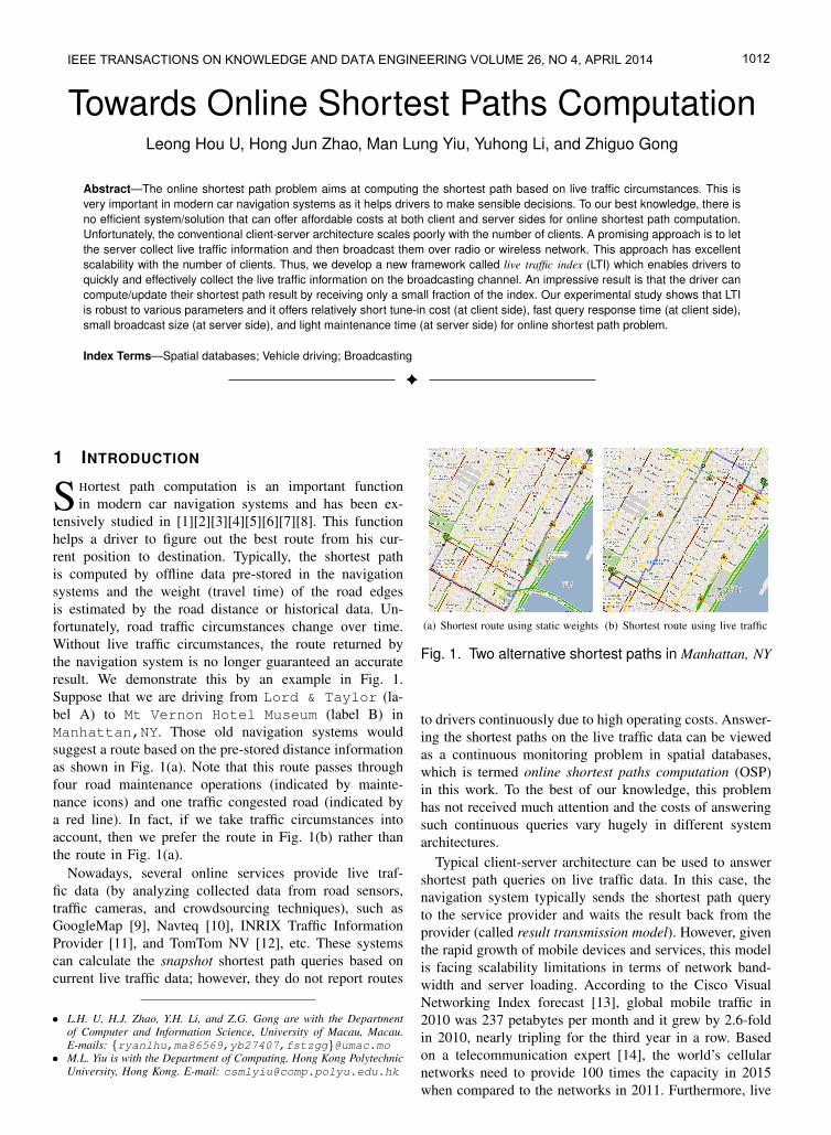
tensively studied in [1][2][3][4][5][6][7][8]. This functionhelps a driver to figure out the best route from his cur-rent position to destination. Typically, the shortest pathis computed by offline data pre-stored in the navigationsystems and the weight (travel time) of the road edgesis estimated by the road distance or historical data. Un-fortunately, road traffic circumstances change over time.Without live traffic circumstances, the route returned bythe navigation system is no longer guaranteed an accurateresult. We demonstrate this by an example in Fig. 1.Suppose that we are driving from Lord & Taylor (la-bel A) to Mt Vernon Hotel Museum (label B) inManhattan,NY. Those old navigation systems wouldsuggest a route based on the pre-stored distance informationas shown in Fig. 1(a). Note that this route passes throughfour road maintenance operations (indicated by mainte-nance icons) and one traffic congested road (indicated bya red line). In fact, if we take traffic circumstances intoaccount, then we prefer the route in Fig. 1(b) rather thanthe route in Fig. 1(a).

Nowadays, several online services provide live traf-fic data (by analyzing collected data from road sensors,traffic cameras, and crowdsourcing techniques), such asGoogleMap [9], Navteq [10], INRIX Traffic InformationProvider [11], and TomTom NV [12], etc. These systemscan calculate the snapshot shortest path queries based oncurrent live traffic data; however, they do not report routes

• L.H. U, H.J. Zhao, Y.H. Li, and Z.G. Gong are with the Departmentof Computer and Information Science, University of Macau, Macau.E-mails: {ryanlhu,ma86569,yb27407,fstzgg}@umac.mo

• M.L. Yiu is with the Department of Computing, Hong Kong PolytechnicUniversity, Hong Kong. E-mail: [email protected]

1

(a) Shortest route using static weights (b) Shortest route using live traffic

Fig. 1. Two alternative shortest paths in Manhattan, NY

to drivers continuously due to high operating costs. Answer-ing the shortest paths on the live traffic data can be viewedas a continuous monitoring problem in spatial databases,which is termed online shortest paths computation (OSP)in this work. To the best of our knowledge, this problemhas not received much attention and the costs of answeringsuch continuous queries vary hugely in different systemarchitectures.

Typical client-server architecture can be used to answershortest path queries on live traffic data. In this case, thenavigation system typically sends the shortest path queryto the service provider and waits the result back from theprovider (called result transmission model). However, giventhe rapid growth of mobile devices and services, this modelis facing scalability limitations in terms of network band-width and server loading. According to the Cisco VisualNetworking Index forecast [13], global mobile traffic in2010 was 237 petabytes per month and it grew by 2.6-foldin 2010, nearly tripling for the third year in a row. Basedon a telecommunication expert [14], the world’s cellularnetworks need to provide 100 times the capacity in 2015when compared to the networks in 2011. Furthermore, live

IEEE TRANSACTIONS ON KNOWLEDGE AND DATA ENGINEERING VOLUME 26, NO 4, APRIL 2014 1012


traffic are updated frequently as these data may be collectedby using crowdsourcing techniques (e.g., anonymous trafficdata from Google map users on certain mobile devices). Assuch, huge communication cost will be spent on sendingresult paths on the this model. Obviously, the client-serverarchitecture will soon become impractical in dealing withmassive live traffic in near future. Ku et al. [15] raise thesame concern in their work which processes spatial queriesin wireless broadcast environments based on Euclideandistance metric.

Malviya et al. [16] developed a client-server system forcontinuous monitoring of registered shortest path queries.For each registered query (s, t), the server first precomputesK different candidate paths from s to t. Then, the serverperiodically updates the travel times on these K paths basedon the latest traffic, and reports the current best path tothe corresponding user. Since this system adopts the client-server architecture, it cannot scale well with a large numberof users, as discussed above. In addition, the reported pathsare approximate results and the system does not provide anyaccuracy guarantee.

An alternative solution is to broadcast live traffic dataover wireless network (e.g., 3G, LTE, Mobile WiMAX,etc.). The navigation system receives the live traffic datafrom the broadcast channel and executes the computationlocally (called raw transmission model). The traffic data arebroadcasted by a sequence of packets for each broadcastcycle. To answer shortest path queries based on live trafficcircumstances, the navigation system must fetch thoseupdated packets for each broadcast cycle. However, as wewill analyze an example in Section 2.2, the probability of apacket being affected by 1% edge updates is 98.77%. Thismeans that clients must fetch almost all broadcast packetsin a broadcast cycle.

The main challenge on answering live shortest paths isscalability, in terms of the number of clients and the amountof live traffic updates. A new and promising solutionto the shortest path computation is to broadcast an airindex over the wireless network (called index transmissionmodel) [17][18]. The main advantages of this model arethat the network overhead is independent of the number ofclients and every client only downloads a portion of theentire road map according to the index information. Forinstance, the proposed index in [17] constitutes a set ofpairwise minimum and maximum traveling costs betweenevery two sub-partitions of the road map. However, thesemethods only solve the scalability issue for the numberof clients but not for the amount of live traffic updates.As reported in [17], the re-computation time of the indextakes 2 hours for the San Francisco (CA) road map. Itis prohibitively expensive to update the index for OSP, inorder to keep up with live traffic circumstances.

Motivated by the lack of off-the-shelf solution for OSP,in this paper we present a new solution based on theindex transmission model by introducing live traffic index(LTI) as the core technique. LTI is expected to providerelatively short tune-in cost (at client side), fast queryresponse time (at client side), small broadcast size (at server

side), and light maintenance time (at server side) for OSP.We summarize LTI features as follows.• The index structure of LTI is optimized by two novel

techniques, graph partitioning and stochastic-basedconstruction, after conducting a thorough analysis thehierarchical index techniques [19][20][21]. To the bestof our knowledge, this is the first work to give a thor-ough cost analysis on the hierarchical index techniquesand apply stochastic process to optimize the indexhierarchical structure. (Section 4)

• LTI selectively fetches data in wireless broadcast envi-ronments, which significantly reduce the tune-in cost.(Section 5)

• LTI efficiently maintains the index for live trafficcircumstances by incorporating Dynamic Shortest PathTree (DSPT) [22] into hierarchial index techniques. Inaddition, a bounded version of DSPT is proposed tofurther reduce the broadcast overhead. (Section 6)

• By incorporating the above features, LTI reduces thetune-in cost up to an order of magnitude as comparedto the state-of-the-art competitors; while it still pro-vides competitive query response time, broadcast size,and maintenance time. To the best of our knowledge,we are the first work that attempts to minimize allthese performance factors for OSP.

The rest of the paper is organized as follows. We firstintroduce main performance factors for evaluating OSPand overview the state-of-the-art shortest path computationmethods in Section 2. The system overview and objectivesof our live traffic index (LTI) are introduced in Section 3.The LTI construction, LTI transmission, and LTI mainte-nance are subsequently discussed in Section 4, Section 5and Section 6, respectively. We summarize our completeframework in Section 7 and evaluate LTI thoroughly inSection 8. Finally, our work is concluded in Section 9.

2 PRELIMINARY

2.1 Performance FactorsThe main performance factors involved in OSP are: (i) tune-in cost (at client side), (ii) broadcast size (at server side),and (iii) maintenance time (at server side), and (iv) queryresponse time (at client side).

In this work, we prioritize the tune-in cost as the main op-timized factor since it affects the duration of client receiversinto active mode and power consumption is essentiallydetermined by the tuning cost (i.e., number of packetsreceived) [17][23]. Shortening the duration of active modeis important since it enables the clients to receive moreservices simultaneously by selective tuning [24]. Theseservices may include providing live weather information,delivering latest promotions in the surrounding area, andmonitoring availability of parking slots at destination. If weminimize the tune-in cost of one service, then we reservemore tune-in time for other services.

The index maintenance time and broadcast size relateto the freshness of the live traffic information. The main-tenance time is the time required to update the index

1013


according to live traffic information. The broadcast sizeis relevant to the latency of receiving the latest indexinformation. As the freshness is one of our main designcriteria, we must provide reasonable costs for these twofactors.

The last factor is the response time at client side. Givena proper index structure, the response time of shortest pathcomputation can be very fast (i.e., few milliseconds on largeroad maps) which is negligible compared to access latencyfor current wireless network speed. The computation alsoconsumes power but their effect is outweighed by commu-nication. It remains, however, an evaluated factor for OSP.

2.2 Adaptation of Existing ApproachesIn this section, we briefly discuss the applicability of thestate-of-the-art shortest path solutions on different trans-mission models. As discussed in the introduction, theresult transmission model scales poorly with respect to thenumber of clients. The communication cost is proportionalto the number of clients (regardless of whether the servertransmits live traffic or result paths to the clients). Thus,we omit this model from the remaining discussion.

2.2.1 Raw transmission modelUnder raw transmission model, the traffic data (i.e., edgeweights) are broadcasted by a set of packets for each broad-cast cycle. Each header stores the latest timestamp of thepackets, so that clients can decide which packets have beenupdated, and only fetch those updated packets in the currentbroadcast cycle. Having downloaded the raw traffic datafrom the broadcast channel, the following methods eitherdirectly calculate the shortest path or efficiently maintaincertain data structure for the shortest path computation.Uninformed search (e.g., Dijkstra’s algorithm) traversesgraph nodes in ascending order of their distances from thesource s, and eventually discovers the shortest path to thedestination t. Bi-directional search (BD) [3] reduces thesearch space by executing Dijkstra’s algorithm simultane-ously forwards from s and backwards from t. As to bediscussed shortly, bi-directional search can also be appliedon some advanced index structures. However, the responsetime is relatively high and the clients may receive largeamount of irrelevant updates due to the transmission model.Goal directed approaches search towards the target by fil-tering out the edges that cannot possibly belong to theshortest path. The filtering procedure requires some pre-computed information. ALT [25] and arc flags (AF) [26]are two representative algorithms in this category.

ALT makes use of A∗ search, landmarks, and triangleinequality [27]. A few landmark nodes are selected and thedistances between each landmark and every node are pre-computed. These pre-computed distances can be exploitedto derive distance bounds for A∗ search on the graph.[28] proposes a lazy update paradigm for ALT (DALT) sothat it can tolerate certain extents of edge weights changeson a dynamic graph. The distance bounds derived fromthe pre-computed information remain correct if no edge

weight becomes lower than the initial weight used at theALT construction. This lazy update paradigm significantlyreduces the index maintenance cost.

Another well known goal directed approach is Arc flags(AF) that partitions the graph into m sub-graphs. For eachedge e, it stores a bitmap B where B[i] is set to true ifand only if a shortest path to a node in the sub-graph istarts with e. During the Dijkstra execution, it only relaxesthose edges for which the bitmap flag of the target node’ssub-graph is true. AF provides reasonable speed-ups, butconsume too much space for large road networks. Thedynamic updates of AF (DAF) has been recently studied in[29]. However, the solution is not practical since the costof updating the bitmap flags is exponential to the numberof edge updates.Dynamic shortest paths tree (DSPT) maintains a tree struc-ture locally for efficient shortest path retrieval. [22] dis-cusses how to maintain a correct shortest paths tree rootedat s after receive a set of edge weight updates to the graphG = (V,E). Finding a shortest path from s to any nodeis computed at O(|V |) time on the shortest paths tree.However, maintaining a tree structure for an edge update issimilar to execute an Dijkstra in the worst case. In addition,DSPT requires to keep a tree structure in every networknode. This overhead makes DSPT infeasible for OSP onthe index transmission model.

2.2.2 Index transmission modelThe index transmission model enables servers to broadcastan index instead of raw traffic data. We review the state-of-the-art indices for shortest path computation and discusstheir applicability on this model.Road map hierarchical approaches try to exploit the hi-erarchical structure to the road map network in a pre-processing step, which can be used to accelerate all sub-sequent queries. These speed-up approaches include reach[4], highway hierarchies (HH) [2][6], contraction hierar-chies (CH) [30], and transit-node routing (TNR) [1].

Reach, HH, and CH are based on shortcut techniques[2][6], i.e., some paths in the original graph are representedby some shortcut edges. The shortcuts are identified out byexploiting the hierarchical structure (e.g., node ordering) onthe road map network. To answer a query, a bi-directionalsearch is executed on the overlay graph that constitutes ofthe shortcuts and some edges in the original graph. As theshortcuts are the only extra structure stored in the index,the construction is relatively fast as compared to other indexapproaches.

TNR is based on a simple observation that a drivingpath only passes one of a few important transit nodes. Foreach shortest path query (s, t), two transit node sets,

−→A (s)

and←−A (t), can be identified by the forward and backward

searches from the source and the destination, respectively.The length of the shortest path (s, t) that passes at leastone transit node is given by min {dist(s, u) +dist(u, v)

+dist(v, t) | u ∈−→A (s), v ∈

←−A (t)}, where all involved

distances can be directly looked up in the pre-computed

1014


data structure. Note that if the shortest path that passes notransit node, then other shortest path algorithm is appliedinstead.

The hierarchical approaches can provide very fast querytime as reported in [31]. However, the maintenance timecould be very high as most of them have no efficient ap-proach to update the pre-computed data structure. HH andCH can support dynamic weight updates [7] but the solutionis limited to weight increasing cases. In [32], a theoreticalapproach has been proposed to update the overlay graphs,but the proposed methods have not been tested in practice.Again, none of these approaches is scalable using the indextransmission model since the shortest path can only becomputed on a complete index.Hierarchical index structures provide another way to ab-stracting and structuring a topographical index in a hierar-chical fashion. Hierarchical MulTi-graph model (HiTi) [21]is a representative approach in this category. The meaningof hierarchy in HiTi is the hierarchy of the index (i.e.,tree structure) instead of the hierarchy of the road map(i.e., level of roads). By exploiting the hierarchical indexstructure, HiTi can support fast shortest path computationon a portion of entire index which can significantly reducethe tune-in cost on the index transmission model. However,prohibitive maintenance time and large broadcast size makeit inapplicable to OSP on any transmission model.

Hierarchical Encoded Path View (HEPV) [20] and Hubindexing [19] share the same intuition of HiTi which divideslarge graph into smaller subgraphs and organize them in ahierarchical fashion by pushing up border nodes. However,both are infeasible for OSP since these approaches sufferfrom the excessive storage overhead for a large amount ofpre-computed path information.

TEDI [33] applies a tree-based partitioning on the roadgraph such that each partition in the tree has a boundednumber of sub-partitions. This method is applicable tounweighted graphs only; it is not applicable to typical roadnetworks where the edges are weighted. Furthermore, thereis no discussion on how to maintain the TEDI structure inpresence of edge weight updates.Oracle Sankaranarayanan et al. [34][35] focus on precom-puting certain shortest path distances called oracles in orderto answer approximate shortest path queries efficiently.These techniques bound the approximate path distance errorto be ε times the shortest path distance. The distanceoracle [34] can answer approximate shortest path distancequery in O(log |V |) time, and it occupies O(|V |/ε2) space.The path oracle [35] takes the same complexity, and itcan compute an approximate shortest path in O(k log |V |)time, where k is the number of vertices on the path. Themaintenance of these oracles regarding live traffic updateshas not been studied in [34][35]. Also, these techniques donot provide exact results and incur high storage space atsmall ε.Full pre-computation pre-computes the shortest paths be-tween any two nodes in the road network, such as SILC [36]and distance index [37]. Even though these approaches

offer fast query response time, the maintenance cost andsize overhead become prohibitive on large road networks.Besides, as reported by [38], the performance of the fullpre-computation approaches (i.e., SILC [36]) is not muchsuperior to those road map hierarchical approaches (i.e.,CH [30]).Combination approaches integrate promising features fromdifferent index structure to support efficient shortest pathcomputation. SHARC [39] and CALT [31] are two wellstudied combination approaches which integrate road maphierarchical approaches with AF and ALT, respectively.However, these complex index structures are either lack ofefficient maintenance strategies or have huge size overheadwhich makes them inapplicable to OSP on any transmissionmodel.

2.2.3 SummaryExcept for hierarchical index structures, all methods oneither raw or index transmission models suffer from adrawback that a few updates could affect a large portionof packets. We demonstrate this by a simple probabilisticanalysis. Suppose that there are B packets in a broadcastcycle and U edges are updated. The probability of a specificpacket being affected by the updates is 1−(1−1/B)U . Forinstance, suppose that the San Francisco (CA) bay area roadnetwork can be transmitted in 1,000 packets (443,604 edgesin total), and there are 1% live traffic updates (i.e., ≈4,400edges) in each processing cycle. Thus, the probability ofa packet being affected is 98.77%. This means that almostevery broadcast packet is updated by this small portion ofedge updates.

Fig. 2 illustrates the relative performance1 to differ-ent cost factors (including tune-in cost, response time,broadcast size, and maintenance time) on two transmissionmodels. Except that BD, DALT, and DSPT use the rawtransmission model, other methods use the index transmis-sion model. Except for HiTi [21] and LTI (our proposedmethod), the tune-in cost of all approaches is very closeto the broadcast size as explained above. Based on thecomparison in Fig. 2, LTI is the only method that supportsrelatively low tune-in cost (at client side), fast query re-sponse time (at client side), small broadcast size (at serverside), and light index maintenance time (at server side) forOSP.

3 LTI OVERVIEW AND OBJECTIVES

3.1 LTI OverviewA road network monitoring system typically consists of aservice provider, a large number of mobile clients (e.g., ve-hicles), and a traffic provider (e.g., GoogleMap, NAVTEQ,INRIX, etc.). Fig.3 shows an architectural overview ofthis system in the context of our live traffic index (LTI)framework. The traffic provider collects the live trafficcircumstances from the traffic monitors via techniques likeroad sensors and traffic video analysis. The service provider

1. based on the experimental results reported by [31] and [38]

1015


1

Broadcast size

Mai

nte

nan

ce t

ime

Ideal

LTICH

BD, DALT, DSPT

CALT

HiTi

SHARC DAF

TNR

SILC

(a) costs at service provider

Tune-in cost

Res

po

nse

tim

e

Ideal

LTI CH

BD, DSPT

CALT

HiTi

SHARC

DAF

TNRSILC

DALT

(b) costs at client

Fig. 2. Relative performance illustration

periodically receives live traffic updates from the trafficprovider and broadcasts the live traffic index on radio orwireless network (e.g., 3G, LTE, Mobile WiMAX, etc.).When a mobile client wishes to compute and monitor ashortest path, it listens to the live traffic index and readsthe relevant portion of the index for deriving the shortestpath.

In this work, we focus on handling traffic updates butnot graph structure updates. For real road networks, it isinfrequent to have graph structure updates (i.e., constructionof a new road) when compared to edge weight updates(i.e., live traffic circumstances). Thus, we assume that thegraph structures are distributed to every client in advance(e.g., by monthly updates or at system boot-up) via typicaltransmission protocol (i.e., HTTP and FTP).

Traffic Provider

Traffic MonitorTraffic Monitor

GPS Air index

head

erda

ta 1

data

2...

data

mhe

ader

data

m+

1da

ta m

+2

...da

ta 2

mhe

ader

...

Service Provider

Road network

Road network

Road network

Road network

Trafficupdates

live traffic

live traffic

Fig. 3. LTI System Overview

In Fig.4, we illustrate the components and system flow inour LTI framework. The components shaded by gray colorare the core of LTI. In order to provide live traffic infor-mation, the server maintains (component a) and broadcasts(component b) the index according to the up-to-date trafficcircumstances. In order to compute the online shortest path,a client listens to the live traffic index, reads the relevantportions of the index (component c), and computes theshortest path (component d).

3.2 LTI Objectives

To optimize the performance of the LTI components, oursolution should support the following features.(1) Efficient maintenance strategy. Without efficientmaintenance strategy, long maintenance time is needed at

Client Service Provider

(c) Tune-in&listen relevant packets

Query q(s,d)

(b) Broadcast index

(a) Maintain index

Receive traffic updates

Traffic Provider

(d) Compute result for q(s,d)

Communication

Computation

Fig. 4. Components in LTI

server side so that the traffic information is no longer live.This can reduce the maintenance time spent at componenta.(2) Light index overhead. The index size must be con-trolled in a reasonable ratio to the entire road map data. Thisreduces not only the length of a broadcast cycle, but alsomakes clients listen fewer packets in the broadcast channel.This can save the communication cost at components b andc.(3) Efficient computation on a portion of entire index.This property enables clients to compute shortest path on aportion of the entire index. The computation at componentd gets improved since it is executed on a smaller graph.This property also reduces the amount of data received andenergy consumed at component c.

Inspired by these properties, LTI has relatively shorttune-in cost (at client side), fast query response time (atclient side), small broadcast size (at server side), andlight index maintenance time (at server side) for OSP. Asdiscussed in Section 2.2, the hierarchical index structuresenable clients to compute the shortest path on a portion ofentire index. However, without pairing up with the first andsecond features, the communication and computation costsare still infeasible for OSP. To achieve these two features,in Section 4 and Section 6, we will discuss how to optimizethe hierarchical structure and efficiently maintain the indexaccording to live traffic circumstances.

4 LTI CONSTRUCTION

In Section 4.1, we carefully analyze the hierarchical indexstructures and study how to optimize the index. In Sec-tion 4.2, we present a stochastic based index constructionthat minimizes not only the size overhead but also reducesthe search space of shortest path queries. To the best ofour knowledge, this is the first work to analyze the hierar-chical index structures and exploit the stochastic process tooptimize the index.

4.1 Analysis of Hierarchical Index StructuresHierarchical index structures (e.g., HiTi [21], HEPV [20],and Hub Indexing [19], TEDI [33]) enable fast shortest pathcomputation on a portion of entire index which significantlyreduces the tune-in cost on the index transmission model.Given a graph G = (VG, EG) (i.e., road network), this typeof index structures partitions G into a set of small sub-graphs SGi and organizes SGi in a hierarchical fashion(i.e., tree). In Fig. 5, we illustrate a graph being partitioned

1016


into 10 subgraphs (SG1, SG2, ..., SG10) and the corre-sponding hierarchical index structure.

1

a

SG1

SG2

e f

g

i

h

b

c d

SG3

nl

mk

j

SG4 SG5

SG6 SG7

SG9 SG10

SG8

o

p

q

r

(a) road network

SG1-2 SG3

SG2SG1

SG4 SG5

SG1-3 SG4-5

SG1-5

SG8 SG9

SG7 SG8-9 SG10SG6

SG6-7 SG8-10

SG6-10

SG1-10

Search Graph of q(b,d)b

d

(b) hierarchical tree view

Fig. 5. Hierarchical index structure

Every leaf entry in a hierarchical structure represents asubgraph SGi that consists of the corresponding nodes andedges from the original graph. For instance, SG1 consists oftwo nodes VSG1

= {a, b} and one edge ESG1= {(a, b)}.

A non-leaf entry stores the inter-connectivity informationbetween the child entries. For instance, SG1-2 stores a con-nectivity edge ΓSG1-2 = {(b, c)} between SG1 and SG2.To boost up the shortest path computation, the hierarchicalindex structures also keep some pre-computed informationin the index entries. For instance, shortcuts ∆SGi

are themost common type of pre-computed information in theseindices, where a shortcut is the shortest path betweentwo border nodes in a subgraph. In Fig. 5, SG5 has twoborder nodes2 k and m so that SG5 keeps a shortcut∆SG5

= {(k,m)} and its corresponding weight.To answer a shortest path query q(s, t) using the hi-

erarchical structures, a common approach is to fetch therelevant entries from the index using a bottom-up executionfashion. For the sake of analysis, we use HiTi as ourreference model in the remaining discussion. Our analysiscan be adapted to other approaches since their executionparadigm shares the same principle.

In Fig. 5, the relevant entries of a shortest path queryq(b, d) are shaded in gray color. Besides the source and des-tination leaf entries (SG1 and SG3), we need to fetch theentries from two leaf entries towards the root entry (SG1-2,SG1-3, SG1-5, and SG1-10) and their sibling entries (SG2,SG4-5, and SG6-10). The shortest path is computed on thesearch graph Gq (typically much smaller than G) whichconstitutes of the edges from the source and destinationentries and the connectivity edges and shortcuts from otherrelevant entries. Note that the edges in Gq already securethe correctness of the shortest path query process [21]. Asan example, suppose the shortest path of q(b, d) passesthrough an edge in SG6, this path must be revealed inthe shortcut of SG6-10 (i.e., ∆SG6-10 = {(f, p)}).Cost analysis. The total space requirement of a hierarchi-cal index I can be represented as follows.

|I| =∑

SGi∈I

(|VSGi |+ |ESGi |+ |ΓSGi |+ |∆SGi |) + tree (1)

where VSGi and ESGi represent the nodes and edges inSGi, respectively, ΓSGi

represents the connectivity infor-mation between the child entries, ∆SGi

represents the pre-computed information kept in SGi, and tree represents the

2. node n is a border node in SG4-5 but not in SG5.

hierarchical information of I . Since VSGi , ESGi and ΓSGi

are directly derived from the original graph and tree isnegligible compared to G, the space requirement can berevised as the follows.

|I| ≈ |G|+∑

SGi∈I

|∆SGi | (2)

To minimize the index broadcast size, it is more or lessequivalent to minimize the size of ∆SGi

. The simplest wayis to partition the graph into multiple subgraphs such thatthe total size of ∆SGi

is minimized. However, this may notoptimize the query performance being discussed shortly.

In our problem, both tune-in cost and query responsetime are highly relevant to the size of the search graph Gq

(i.e., search space). Given an index I and a query q, thesearch space of q can be represented by the relevant edgesets.

S(I, q) = |ESGs ∪ ESGt ∪ {ΓSGi ∪∆SGi : ∀SGi ∈ Gq−st}|(3)

where SGs and SGt represent the leaf entry of sourceand destination, respectively and Gq−st = Gq \ {SGs ∪SGt}. To reduce S(I, q) for all possible queries, our goalis to find a hierarchical structure such that it minimizes(O1) the size of leaf entries ESGs and ESGt , (O2) theoverhead of pre-computed information ∆SGi

, and (O3) thenumber of relevant entries Gq . However, these objectivesare correlated to each other. For instance, to make ESGs

and ESGt smaller, a simple way is to partition G into moresubgraphs; however, it may increase the number of relevantentries Gq and the number of border nodes ∆SGi

.

4.2 Index ConstructionThe above discussion shows that it is hard to find ahierarchical index structure I that achieves all optimizationobjectives. One possible solution is to relax the optimizationobjectives which makes them be the tunable factors of theproblem. While the overhead of pre-computed information(O2) and the number of relevant entries (O3) cannotbe decided straightforwardly, we decide to relax the firstobjective (i.e., minimizing the size of leaf entries) such thatit becomes a tunable factor in constructing the index.

To minimize the overhead of pre-computed information(O2), we study a graph partitioning optimization thatminimizes the index overhead ∆SGi

through the entireindex construction subject to a leaf entry constraint (O1).Subsequently, we propose a stochastic process to optimizethe index structure such that the size of the query searchgraph Gq is minimized (O3).Graph partitioning optimization. For the sake of discus-sion, we denote that the number of subgraphs being createdis γ that is a tunable parameter for controlling the number ofsubgraphs 3 in this work. According to Eq. 2, minimizingthe size of ∆SGi is likely to minimize the overhead ofI . Obviously, our objective is to find a hierarchical indexstructure I such that

OBJ (I) = minSGi∈I

∑|∆SGi |

min{|VSGi |}(4)

3. γ can be viewed as a parameter to control the size of subgraphs.

1017


where min{|VSGi|} can be viewed as a normalized factor

such that the objective function prefers balanced partitions.We observe that minimizing Eq. 4 is similar to finding

the best Cheeger cut [40] in a graph. A Cheeger cut is toremove some edges from a graph such that the graph isisolated into n subgraphs subject to an objective function:

OBJ Cheeger(G) = minSG1,...,SGn∈G

Cut({SG1, ..., SGn})min{|SG1|, ..., |SGn|}

(5)where Cut({SG1, ..., SGn}) is the number of edges be-tween any two subgraphs.

We use an example to illustrate how Cheeger cutresult can be viewed as a good result of I . Fig.6(a)shows a Cheeger cut on a graph where the cut valueCut({SG1, SG2}) and the number of shortcut edges,|∆SG1

| + |∆SG2| = |{∅}| + |{(e, f), (e, g), (f, g)}|, are

identical (i.e., 3). A large cut value is likely to producemore shortcut edges; in Fig.6(b), the cut value is 10 andthere are 12 shortcuts.

1

cut

SG1 SG2

d

e

f

g

a b

c

h

i

j

(a) 3 shortcut edges

cut

SG1

SG2

d

e

f

g

a b

c

h

i

j

(b) 24 shortcut edges

Fig. 6. The number of shortcut edges created bydifferent cuts

Lemma 1: Given a cut having the cut value c and themaximum cut degree of border nodes dcut (where the cutdegree only counts on those edges being cut), the numberof shortcuts produced by the cut is bounded by c(c−1)

2 +(c−dcut+1)(c−dcut)

2 .Proof: Given a cut having the cut value c and the

maximum cut degree dcut, the maximum number of bordernodes in two subgraphs being created is c and c−dcut+1,respectively. Thereby, the maximum number of shortcutsbeing created is c(c−1)

2 + (c−dcut+1)(c−dcut)2 .

Lemma 1 provides a relationship between the Cheegercut and our objective function. Practically, the effect of dcutis negligible since dcut is relatively small as compared to c.For instance, the average in/out degree of the San Francisco(CA) bay area vertices is only 2.54 (which means dcut issmaller than 2.54 since a portion of these edges are interioredges.). Therefore, we claim that a partitioning result thatminimizes Eq. 5 is likely to minimize Eq. 4 as well.

Finding the best Cheeger cut can be reduced to aquadratic discrete optimization problem [41]. Based on[41], a cut on a graph can be determined by the secondsmallest eigenvalue λ and its corresponding eigenvector V .The problem becomes to decompose V into two subsetssuch that the objective function is minimized. To furtherimprove the quality of each cut, we use Eq. 4 as the objec-tive function so that we can heuristically reduce the numberof border nodes. To construct an index, we recursively cutthe subgraphs until we have enough partitions (i.e., the leaf

entry constraint, γ). The pseudo code is omitted due tospace limits.

Stochastic based index construction. The graph parti-tioning framework only returns a binary tree index Ibi thatis constructed based on Cheeger cut sequences. However,Ibi only fulfills the first two objectives (i.e., minimizingthe overhead |∆SGi | subject to γ). Intuitively, the size ofsearch graphs Gq (i.e., O3) is highly relevant to the indexhierarchical structure. As a motivating example, the numberof relevant entries of q(b, d) is reduced from 9 to 8 if weremove one index node (e.g., SG1−2) from the index treein Fig. 5(b). The new index and the relevant entries areillustrated in Fig. 7.

SG2 SG3SG1 SG4 SG5

SG1-3 SG4-5

SG1-5

SG8 SG9

SG7 SG8-9 SG10SG6

SG6-7 SG8-10

SG6-10

SG1-10

Search Graph of q(b,d)

b d

Fig. 7. Effect of hierarchical structure

Given the size of leaf entries γ, minimizing the sizeof search graph can be viewed as a problem of findingthe best hierarchical index structure for potential queries.Finding the optimal hierarchical structure is challengingsince (1) the performance of an index cannot be easilyestimated (which should be estimated by a query workloadQ or a universal query set U) and (2) the index statistics(e.g., shortcuts) are changed on different index hierarchicalstructures (which is necessarily recalculated based on thestructure). This problem is similar to those combinatorialoptimization problems (e.g., hierarchical clustering [42])that groups data into a set of hierarchical partitions suchthat the objective function is optimized. Typically, thesecombinatorial problems are solved by approximate solu-tions under reasonable response time. Thus, we propose atop-down approach that greedily decides the structure basedon a stochastic estimation.

To estimate the average size of the search graphs, weapply a stochastic process, Monte Carlo, that relies onrandom sampling to obtain numerical results. In this work,the Monte Carlo process is to execute a set of randomlygenerated shortest path queries on a temporal index I ′

and estimates the average size of their relevant searchgraphs, avg(S(I ′)). For clarity, the stochastic process canbe replaced by a query workload, Q, based estimationwhich should offer more accurate estimation when Q isavailable.

At every partitioning, we attempt to find the best structurefor the potential queries by the stochastic process. Morespecifically, we assess the average size of the relevantsearch graphs, avg(S(I ′)), for different partitioning settings(i.e., varying k). Among all assessed partitioning, we attachthe partitioning having the smallest relevant search graphsto the index. The construction terminates when we haveenough leave entries (i.e., γ). Algorithm 1 shows the pseudo

1018


codes of the partitioning algorithm based on the stochasticprocess.

Algorithm 1 Stochastic Partitioning AlgorithmPQ: a priority queue; I: index structure;Algorithm partition(G:the graph, γ:the number of partitions)

1: (λ,V) := eigen(G) and n := root of I2: insert (n,G,V, λ) into PQ in decreasing order to λ3: while |PQ| < γ do4: (n,G,V, λ) := PQ.pop()5: for k:=2 to γ − |PQ|+ 1 do6: decompose G into SG1...SGk s.t. Eq. 4 is minimized7: form a temporal index I′ that attaches SG1...SGk

8: if avg(S(I′)) is better than bestS then9: update bestS and bestSG := {SG1, ..., SGk}

10: attach bestSG as n’s children11: for i:=1 to |bestSG| do12: insert (ni, SGi,Vi, λi) into PQ13: return I

The effect of γ. In this work, LTI requires only oneparameter γ to construct the index which is used to controlthe number of subgraphs being constructed. Our proposedtechniques attempt to optimize the index (O2 and O3)subject to γ. Intuitively, similar to other hierarchical indices,the number of leaf entries, γ, not only affects the size ofleaf entries but also the search performance.

1

SG1 SG2

SG1-2

s t

(a) small γ

SG1 SG2 SG3 SG4

SG1-2 SG3-4

SG1-4

s t

(b) large γ

Fig. 8. The effect of γ on index construction

Fig. 8 illustrates a toy example that shows the effect ofγ in different settings. Obviously, when γ is set to a largevalue, the index has small size of leaf entries (i.e., ESGs

and ESGt ) which boost the query processing due to thelocality of relevant entries. However, it may increase thenumber of relevant entries to answer queries due to thehierarchy of the index. In summary, a small γ may leadthe index having large leaf entries while a large γ may leadthe index having large number of index nodes, where thesesettings may degrade the query performance. Fortunately,γ is not a very sensitive parameter (cf. the studies inother hierarchical indexing techniques [19][20][21] and ourexperiments), which can be decided by experimental studiesin practice.

5 LTI TRANSMISSIONIn this section, we present how to transmit LTI on the airindex. We first introduce a popular broadcasting schemecalled the (1,m) interleaving scheme in Section 5.1. Basedon this broadcasting scheme, we study how to broadcast LTIin Section 5.2 and how a client receives edge updates onair in Section 5.3.

5.1 Broadcasting SchemeThe broadcasting model uses radio or wireless network(e.g., 3G, LTE, Mobile WiMAX) as the transmission

medium. When the server broadcasts a dataset (i.e., a “pro-gramme”), all clients can listen to the dataset concurrently.Thus, this transmission model scales well independent ofthe number of clients. A broadcasting scheme is a protocolto be followed by the server and the clients.

TABLE 1The format of the (1,m) interleaving scheme

header data header data header datai:0, n:6 o1, o2 i:2, n:6 o3, o4 i:4, n:6 o5, o6

The (1,m) interleaving scheme [23] is one of the bestbroadcasting schemes. Table 1 shows an example broad-casting cycle with m = 3 packets and the entire datasetcontains 6 data items. First, the server partitions the datasetinto m equi-sized data segments. Each packet containsa header and a data segment, where a header describesthe broadcasting schedule of all packets. In this example,the variables i and n in each header represent the lastbroadcasted item and the total number of items. The serverperiodically broadcasts a sequence of packets (called as abroadcast cycle).

We use a concrete example to demonstrate how a clientreceives her data from the broadcast channel. Suppose thata client wishes to query for the data object o5. First, theclient tunes in the broadcast channel and waits until the nextheader is broadcasted. For instance, the client is listeningto the header of the first packet, and finds out that the thirdpacket contains o5. In order to preserve energy, the clientsleeps until the broadcasting time of that packet. Then, itwake-ups and reads the requested data item from the packet.

The query performance can be measured by the tuningtime and the waiting time at the client side. The tuning timeis the time for reading the packets. The waiting time is thetime from the start time to the termination time of the query.In this broadcasting scheme, the parameter m decides thetrade-off between tune-in size and the overhead. A large mfavors small tune-in size whereas a small m incurs smallwaiting time. [23] suggests to set m to the square root ofthe ratio of the data size to the index size.

5.2 LTI on AirTo broadcast a hierarchical index using the (1,m) in-terleaving scheme, we first partition the index into twocomponents: the index structure and the weight of edges.The former stores the index structure (e.g., graph vertices,graph edges, and shortcut edges) and the latter stores theweight of edges. In order to keep the freshness of LTI, oursystem is required to broadcast the latest weight of edgesperiodically 4.

Table 2 shows the format of a header/data packet inour model. id is the offset of the packet in the presentbroadcast cycle and checksum is used for error-checkingof the header and data. Note that the packet does notstore any offset information to the next broadcast cycle or

4. The hierarchical index structure is only affected by the connectivity /topology information (see Sections 4 and Sections 6). Thus, any changesin the weights would not affect the hierarchical index structure.

1019


TABLE 2Packet format on the air index

Offset 1 2 3 4 5 6 7 8 9 10 11 12 13 14 15 160 id checksum ...... ...

broadcast segment. The offset can be matched up by thecorresponding id since the structure of LTI is pre-storedat each client. In our model, the header packet stores atimestamp set T for checking new updates and data lossrecovery.

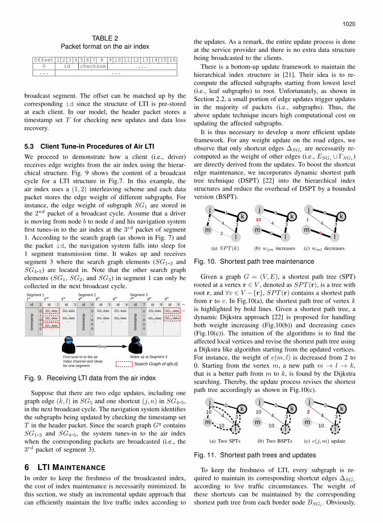
5.3 Client Tune-in Procedures of Air LTIWe proceed to demonstrate how a client (i.e., driver)receives edge weights from the air index using the hierar-chical structure. Fig. 9 shows the content of a broadcastcycle for a LTI structure in Fig.7. In this example, theair index uses a (1, 2) interleaving scheme and each datapacket stores the edge weight of different subgraphs. Forinstance, the edge weight of subgraph SG1 are stored inthe 2nd packet of a broadcast cycle. Assume that a driveris moving from node b to node d and his navigation systemfirst tunes-in to the air index at the 3rd packet of segment1. According to the search graph (as shown in Fig. 7) andthe packet id, the navigation system falls into sleep for1 segment transmission time. It wakes up and receivessegment 3 where the search graph elements (SG1-3 andSG4-5) are located in. Note that the other search graphelements (SG1, SG2, and SG3) in segment 1 can only becollected in the next broadcast cycle.

0i000...

SG1 data…

SG2 data…

SG3 data…

SG4 data...

SG5 data…

SG6 data...

SG7 data…

SG7 data...

SG8 data…

SG9 data…

SG10 data…

SG1-3 data...

SG4-5 data…

Segment 1 Segment 2 Segment 3

id 1 id 2 id 3 id 4 id 5 id 6 id 7 id 8 id 9

times

tam

p

0i000...

times

tam

p

0i000...

times

tam

p

...

...

1st 2nd 3rd 4th 5th 6th 7th 8th 9th

First tune-in to the air index channel and sleep for one segment

Wake up at Segment 3

Sleep

Search Graph of q(b,d)

Fig. 9. Receiving LTI data from the air index

Suppose that there are two edge updates, including onegraph edge (k, l) in SG5 and one shortcut (j, n) in SG4-5,in the next broadcast cycle. The navigation system identifiesthe subgraphs being updated by checking the timestamp setT in the header packet. Since the search graph Gq containsSG1-3 and SG4-5, the system tunes-in to the air indexwhen the corresponding packets are broadcasted (i.e., the3rd packet of segment 3).

6 LTI MAINTENANCE

In order to keep the freshness of the broadcasted index,the cost of index maintenance is necessarily minimized. Inthis section, we study an incremental update approach thatcan efficiently maintain the live traffic index according to

the updates. As a remark, the entire update process is doneat the service provider and there is no extra data structurebeing broadcasted to the clients.

There is a bottom-up update framework to maintain thehierarchical index structure in [21]. Their idea is to re-compute the affected subgraphs starting from lowest level(i.e., leaf subgraphs) to root. Unfortunately, as shown inSection 2.2, a small portion of edge updates trigger updatesin the majority of packets (i.e., subgraphs). Thus, theabove update technique incurs high computational cost onupdating the affected subgraphs.

It is thus necessary to develop a more efficient updateframework. For any weight update on the road edges, weobserve that only shortcut edges ∆SGi are necessarily re-computed as the weight of other edges (i.e., ESGi

∪ΓSGi)

are directly derived from the updates. To boost the shortcutedge maintenance, we incorporates dynamic shortest pathtree technique (DSPT) [22] into the hierarchical indexstructures and reduce the overhead of DSPT by a boundedversion (BSPT).

1

3

3

l

4

2

1

m

kj

(a) SPT (k)

3

34

2

10

m

k

l

j

(b) wjm increases

3

3

j

4

0

1

m

k

l

(c) wml decreases

Fig. 10. Shortest path tree maintenance

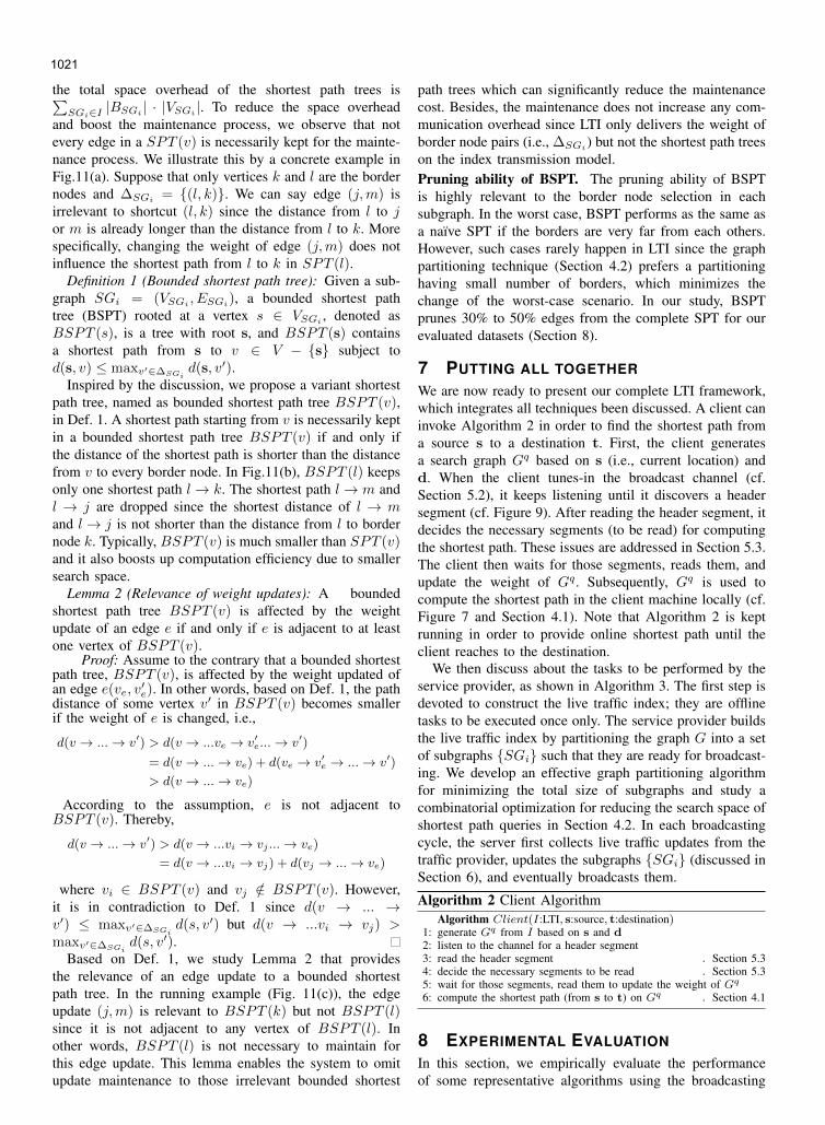
Given a graph G = (V,E), a shortest path tree (SPT)rooted at a vertex r ∈ V , denoted as SPT (r), is a tree withroot r, and ∀v ∈ V −{r}, SPT (r) contains a shortest pathfrom r to v. In Fig.10(a), the shortest path tree of vertex kis highlighted by bold lines. Given a shortest path tree, adynamic Dijkstra approach [22] is proposed for handlingboth weight increasing (Fig.10(b)) and decreasing cases(Fig.10(c)). The intuition of the algorithms is to find theaffected local vertices and revise the shortest path tree usinga Dijkstra like algorithm starting from the updated vertices.For instance, the weight of e(m, l) is decreased from 2 to0. Starting from the vertex m, a new path m → l → k,that is a better path from m to k, is found by the Dijkstrasearching. Thereby, the update process revises the shortestpath tree accordingly as shown in Fig.10(c).

1

2

34

10

10

lm

kj

(a) Two SPTs

2

34

10

10

lm

kj

(b) Two BSPTs

2

34

10

2

lm

kj

(c) e(j,m) update

Fig. 11. Shortest path trees and updates

To keep the freshness of LTI, every subgraph is re-quired to maintain its corresponding shortcut edges ∆SGi

according to live traffic circumstances. The weight ofthese shortcuts can be maintained by the correspondingshortest path tree from each border node BSGi

. Obviously,

1020


the total space overhead of the shortest path trees is∑SGi∈I |BSGi | · |VSGi |. To reduce the space overhead

and boost the maintenance process, we observe that notevery edge in a SPT (v) is necessarily kept for the mainte-nance process. We illustrate this by a concrete example inFig.11(a). Suppose that only vertices k and l are the bordernodes and ∆SGi

= {(l, k)}. We can say edge (j,m) isirrelevant to shortcut (l, k) since the distance from l to jor m is already longer than the distance from l to k. Morespecifically, changing the weight of edge (j,m) does notinfluence the shortest path from l to k in SPT (l).

Definition 1 (Bounded shortest path tree): Given a sub-graph SGi = (VSGi , ESGi), a bounded shortest pathtree (BSPT) rooted at a vertex s ∈ VSGi , denoted asBSPT (s), is a tree with root s, and BSPT (s) containsa shortest path from s to v ∈ V − {s} subject tod(s, v) ≤ maxv′∈∆SGi

d(s, v′).Inspired by the discussion, we propose a variant shortest

path tree, named as bounded shortest path tree BSPT (v),in Def. 1. A shortest path starting from v is necessarily keptin a bounded shortest path tree BSPT (v) if and only ifthe distance of the shortest path is shorter than the distancefrom v to every border node. In Fig.11(b), BSPT (l) keepsonly one shortest path l→ k. The shortest path l→ m andl → j are dropped since the shortest distance of l → mand l→ j is not shorter than the distance from l to bordernode k. Typically, BSPT (v) is much smaller than SPT (v)and it also boosts up computation efficiency due to smallersearch space.

Lemma 2 (Relevance of weight updates): A boundedshortest path tree BSPT (v) is affected by the weightupdate of an edge e if and only if e is adjacent to at leastone vertex of BSPT (v).

Proof: Assume to the contrary that a bounded shortestpath tree, BSPT (v), is affected by the weight updated ofan edge e(ve, v′e). In other words, based on Def. 1, the pathdistance of some vertex v′ in BSPT (v) becomes smallerif the weight of e is changed, i.e.,

d(v → ...→ v′) > d(v → ...ve → v′e...→ v′)

= d(v → ...→ ve) + d(ve → v′e → ...→ v′)

> d(v → ...→ ve)

According to the assumption, e is not adjacent toBSPT (v). Thereby,

d(v → ...→ v′) > d(v → ...vi → vj ...→ ve)

= d(v → ...vi → vj) + d(vj → ...→ ve)

where vi ∈ BSPT (v) and vj /∈ BSPT (v). However,it is in contradiction to Def. 1 since d(v → ... →v′) ≤ maxv′∈∆SGi

d(s, v′) but d(v → ...vi → vj) >maxv′∈∆SGi

d(s, v′).Based on Def. 1, we study Lemma 2 that provides

the relevance of an edge update to a bounded shortestpath tree. In the running example (Fig. 11(c)), the edgeupdate (j,m) is relevant to BSPT (k) but not BSPT (l)since it is not adjacent to any vertex of BSPT (l). Inother words, BSPT (l) is not necessary to maintain forthis edge update. This lemma enables the system to omitupdate maintenance to those irrelevant bounded shortest

path trees which can significantly reduce the maintenancecost. Besides, the maintenance does not increase any com-munication overhead since LTI only delivers the weight ofborder node pairs (i.e., ∆SGi

) but not the shortest path treeson the index transmission model.Pruning ability of BSPT. The pruning ability of BSPTis highly relevant to the border node selection in eachsubgraph. In the worst case, BSPT performs as the same asa naıve SPT if the borders are very far from each others.However, such cases rarely happen in LTI since the graphpartitioning technique (Section 4.2) prefers a partitioninghaving small number of borders, which minimizes thechange of the worst-case scenario. In our study, BSPTprunes 30% to 50% edges from the complete SPT for ourevaluated datasets (Section 8).

7 PUTTING ALL TOGETHERWe are now ready to present our complete LTI framework,which integrates all techniques been discussed. A client caninvoke Algorithm 2 in order to find the shortest path froma source s to a destination t. First, the client generatesa search graph Gq based on s (i.e., current location) andd. When the client tunes-in the broadcast channel (cf.Section 5.2), it keeps listening until it discovers a headersegment (cf. Figure 9). After reading the header segment, itdecides the necessary segments (to be read) for computingthe shortest path. These issues are addressed in Section 5.3.The client then waits for those segments, reads them, andupdate the weight of Gq . Subsequently, Gq is used tocompute the shortest path in the client machine locally (cf.Figure 7 and Section 4.1). Note that Algorithm 2 is keptrunning in order to provide online shortest path until theclient reaches to the destination.

We then discuss about the tasks to be performed by theservice provider, as shown in Algorithm 3. The first step isdevoted to construct the live traffic index; they are offlinetasks to be executed once only. The service provider buildsthe live traffic index by partitioning the graph G into a setof subgraphs {SGi} such that they are ready for broadcast-ing. We develop an effective graph partitioning algorithmfor minimizing the total size of subgraphs and study acombinatorial optimization for reducing the search space ofshortest path queries in Section 4.2. In each broadcastingcycle, the server first collects live traffic updates from thetraffic provider, updates the subgraphs {SGi} (discussed inSection 6), and eventually broadcasts them.

Algorithm 2 Client AlgorithmAlgorithm Client(I:LTI, s:source, t:destination)

1: generate Gq from I based on s and d2: listen to the channel for a header segment3: read the header segment . Section 5.34: decide the necessary segments to be read . Section 5.35: wait for those segments, read them to update the weight of Gq

6: compute the shortest path (from s to t) on Gq . Section 4.1

8 EXPERIMENTAL EVALUATIONIn this section, we empirically evaluate the performanceof some representative algorithms using the broadcasting

1021


Algorithm 3 Service AlgorithmAlgorithm Service(G:graph)

1: construct I and {SGi} based on G . Section 4.22: for each broadcast cycle do3: collect traffic updates from the traffic provider4: update the subgraphs {SGi} . Section 65: broadcast the subgraphs {SGi} . Section 5.2

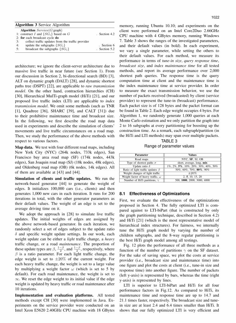
architecture; we ignore the client-server architecture due tomassive live traffic in near future (see Section 1). Fromour discussion in Section 2, bi-directional search (BD) [3],ALT on dynamic graph (DALT) [28], and dynamic shortestpaths tree (DSPT) [22], are applicable to raw transmissionmodel. On the other hand, contraction hierarchies (CH)[30], Hierarchical MulTi-graph model (HiTi) [21], and ourproposed live traffic index (LTI) are applicable to indextransmission model. We omit some methods (such as TNR[1], Quadtree [36], SHARC [39], and CALT [31]) dueto their prohibitive maintenance time and broadcast size.In the following, we first describe the road map dataused in experiments and describe the simulation of clients’movements and live traffic circumstances on a road map.Then, we study the performance of the above methods withrespect to various factors.

Map data. We test with four different road maps, includingNew York City (NYC) (264k nodes, 733k edges), SanFrancisco bay area road map (SF) (174k nodes, 443kedges), San Joaquin road map (SJ) (18k nodes, 48k edges),and Oldenburg road map (OB) (6k nodes, 14k edges). Allof them are available at [43] and [44].

Simulation of clients and traffic updates. We run thenetwork-based generator [44] to generate the weight ofedges. It initializes 100,000 cars (i.e., clients) and thengenerates 1,000 new cars in each iteration. It runs for 200iterations in total, with the other generator parameters astheir default values. The weight of an edge is set to theaverage driving time on it.

We adopt the approach in [28] to simulate live trafficupdates. The initial weights of edges are assigned bythe above network-based generator. In each iteration, werandomly select a set of edges subject to the update ratioδ and specific weight update settings. In our work, eachweight update can be either a light traffic change, a heavytraffic change, or a road maintenance. The proportion ofthese update types are β, 1−β

2 , and 1−β2 , respectively, where

β is a ratio parameter. For each light traffic change, theedge weight is set to ±20% of the current weight. Foreach heavy traffic change, the weight is set to a large valueby multiplying a weight factor ω (which is set to 5 bydefault). For each road maintenance, the weight is set to∞. We reset the edge weight to its initial value if the edgeweight is updated by heavy traffic or road maintenance after10 iterations.

Implementation and evaluation platforms. All testedmethods except CH [30] were implemented in Java. Ex-periments on the service provider were conducted on anIntel Xeon E5620 2.40GHz CPU machine with 18 GBytes

memory, running Ubuntu 10.10; and experiments on theclient were performed on an Intel Core2Duo 2.66GHzCPU machine with 4 GBytes memory, running Windows7. Table 3 shows the ranges of the investigated parameters,and their default values (in bold). In each experiment,we vary a single parameter, while setting the others totheir default values. For each method, we measure itsperformance in terms of tune-in size, query response time,broadcast size, and index maintenance time for all testedmethods, and report its average performance over 2,000shortest path queries. The response time is the querycomputation time at client and the maintenance time isthe index maintenance time at service provider. In orderto measure the exact transmission behavior, we use thenumber of packets received (broadcasted) by client (serviceprovider) to represent the tune-in (broadcast) performance.Each packet size is of 128 bytes and the packet format canbe found in Table 2. Each edge weight occupies 4 bytes. ForAlgorithm 1, we randomly generate 1,000 queries at eachMonte Carlo estimation and we only partition the graph into2 to 16 subgraphs at every partitioning for boosting up theconstruction time. As a remark, each subgraph/partition (inthe HiTi and LTI methods) may span over multiple packets.

TABLE 3Range of parameter values

Parameter ValuesRoad maps NYC, SF, SJ, OB

Type of shortest paths σ short, average, long, mixUpdate ratio δ 1%, 2%, 5%, 10%, 20%, 30%, 40%, 50%

Ratio of light traffic updates β 50%, 60%, 70%, 80%, 90%Weight changes of light traffic ±20%

Weight factor of heavy traffic, ω 2, 5, 10, 15, 20Number of HiTi partitions, γ 500, 1000, 2000, 3000, 4000

8.1 Effectiveness of Optimizations

First, we evaluate the effectiveness of the optimizationsproposed in Section 4. The fully optimized LTI is com-pared against to LTI-biPart (that is constructed by onlythe graph partitioning technique, described in Section 4.2)and HiTi [21] (which is the most representative model ofhierarchical index structures). For fairness, we internallytune the HiTi graph model by varying the number ofchildren subgraphs, and the 8-way regular partitioning isthe best HiTi graph model among all testings.

Fig. 12 plots the performance of all three methods as afunction of the number of partitions γ on the SF dataset.For the sake of saving space, we plot the costs at serviceprovider (i.e., broadcast size and maintenance time) intoone figure and plot the costs at client (i.e., tune-in size andresponse time) into another figure. The number of packets(left y-axis) is represented by bars, whereas the time (righty-axis) is represented by lines.

LTI is superior to LTI-biPart and HiTi for all fourperformance factors in Fig.12. As compared to HiTi, itsmaintenance time and response time are up to 14.7 and21.1 times faster, respectively. The broadcast size and tune-in size are at least 2.4 and 6.4 times smaller than HiTi. Itshows that our fully optimized LTI is very efficient and

1022


10-1

100

101

102

103

104

105

106

Main

tain

tim

e (

ms)

0

20

40

60

80

100

120

140

Bro

adca

st s

ize (

#pack

ets

x 1

00

0)

500 1000 2000 3000 4000

Number of partitions, γ

HiTiLTI-biPartLTI

HiTiLTI-biPartLTI

(a) service provider

10-1

100

101

102

103

Resp

onse

tim

e (

ms)

0

10

20

30

40

50

Tune-i

n s

ize (

#pack

ets

x 1

00

0)

500 1000 2000 3000 4000

Number of partitions, γ

HiTiLTI-biPartLTI

HiTiLTI-biPartLTI

(b) client

Fig. 12. Varying number of partitions, γ

performs vastly different from HiTi. In this work, we set γto 1,000 since it performs the best in both HiTi and LTI. Asshown in the figures, all performance factors are not verysensitive to γ which supports our claim in Section 4.2.

8.2 Scalability experiments

TABLE 4Performance of different methods

Client side: Tune-in cost (#packets), Response time (ms)Server side: Broadcast size (#packets), Maintenance time (ms)

MethodCity raw transmission model index transmission model

BD DALT DSPT CH HiTi LTI

NYC

T 18300.7 18300.7 18300.7 18617.9 26834.5 704.7R 72.39 54.53 374.93 2.28 157.11 4.26B 22930 22930 22930 24802 124870 30661M - - - 15759.6 105451 5575.4

SF

T 11149.4 11149.4 11149.4 10212.1 12468.9 602.8R 89.74 45.03 94.51 0.72 75.89 2.40B 13863 13863 13863 13453 52377 18850M - - - 5411.4 19264.4 2094.9

SJ

T 1191.2 1191.2 1191.2 624.0 1524.1 331.1R 5.20 1.98 9.37 0.08 10.72 1.37B 2525 2525 2525 1370 4602 2827M - - - 276.3 735.3 96.6

OB

T 352.0 352.0 352.0 258.9 516.3 118.4R 1.11 0.45 31.12 0.091 3.66 0.68B 604 604 604 348 1336 666M - - - 104.3 134.6 16.0

Next, we compare the discussed solutions on four differ-ent road maps. The result is shown in Table 4. Note thatall methods on the raw transmission model have the sametune-in size and broadcast size. The only difference is theresponse time as it represents the local computation timefor each client. Apart from BD and DALT, other methodsrequire each client to maintain some index structures locallyafter receiving the live traffic updates. Thus, their responsetime is slower5 than BD and DALT on the raw transmissionmodel. Based on the response time, DALT is the bestapproach among the methods in this category.

Regarding the index transmission model, HiTi is ob-viously infeasible for online shortest path computationdue to its prohibitive costs. Although CH has slightlybetter broadcast size and response time6, we recommendLTI as the best approach due to its light tune-in costand fast maintenance time. The tune-in size significantlyaffects the energy consumption and the duration of active

5. We omit the performance of CH, HiTi, and LTI on the raw transmis-sion model since they are 2 orders of magnitude slower than DALT.

6. We use the codes provided by [30] to construct the CH index whichis implemented in C++ instead of Java.

mode at client receiver. The tune-in size of LTI is 2.19-26.41 and 2.97-25.97 times smaller than CH and DALT,respectively. Note that the margin becomes more significanton larger maps which demonstrates good scalability of ourLTI framework. This is important since reducing the tune-in cost provides opportunity for clients to receive moreservices simultaneously by selective tuning. In addition, fastmaintenance time keeps the freshness of the broadcastedindex. The maintenance time of LTI is 2.58-6.5 times fasterthan CH while the broadcast size of LTI is just 23.6% and40% larger than CH in NYC and SF, respectively.

In Section 1, we show that the present traffic providersreport the traffic very frequently and megabit wirelessnetworks (3G, LTE, Mobile WiMAX, etc.) are available.Therefore, the maintenance time of LTI (i.e., 2 and 5.5seconds on SF and NYC, respectively) is affordable ascompared to the live traffic update frequency and thebroadcast overhead of LTI (i.e., around 35% larger thanthe raw data) is reasonable as the data is transmitted on themegabit wireless networks.

1

10-1

100

101

102

Resp

onse

tim

e (

ms)

0

5

10

15

20

25

30

35

40

Tune-i

n s

ize (

#pack

ets

x 1

00

0)

1% 2% 5% 10% 20% 30% 40% 50%

Update ratio, δ

DALTCHLTI

DALTCHLTI

(a) varying δ

10-1

100

101

102

103

Resp

onse

tim

e (

ms)

0

5

10

15

20

25

Tune-i

n s

ize (

#pack

ets

x 1

00

0)

Short Average Long

Type of shortest paths, σ

DALTCHLTI

DALTCHLTI

(b) varying σ

10-1

100

101

102

Resp

onse

tim

e (

ms)

0

5

10

15

20

25

30

Tune-i

n s

ize (

#pack

ets

x 1

00

0)

50% 60% 70% 80% 90%

Ratio of light traffic updates, β

DALTCHLTI

DALTCHLTI

(c) varying β

10-1

100

101

102

Resp

onse

tim

e (

ms)

0

5

10

15

20

25

30

Tune-i

n s

ize (

#pack

ets

x 1

00

0)

2 5 10 15 20

Weight factor of heavy traffic, ω

DALTCHLTI

DALTCHLTI

(d) varying ω

Fig. 13. Scalability experiments (client)

We omit HiTi from the remaining experiments as it isinferior to LTI. The remaining representative methods are:DALT on the raw transmission model, CH and LTI on theindex transmission model. We evaluate the performanceof these three methods as a function of different systemsettings in Fig.13. In Fig.13(a), the tune-in size of allmethods grow with the update ratio δ, as well, the responsetime slightly increases since the search graph becomeslarger. When δ = 20%, the number of necessary packetsreceived by clients is 13847.2, 13390.12, and 727.28 forDALT, CH, and LTI respectively. DALT and CH almostreceive the entire broadcast packets (i.e., 99.89% and99.53%, respectively); this conforms with our edge-updateprobability analysis in Section 2.2. An impressive finding isthat the client using LTI only receives 20.63% more packetsas compared to δ = 10%. This shows that LTI is robust asthe tune-in size only increases sub-linearly with the updateratio δ.

1023


Fig.13(b) shows the tune-in size and response time ofthe methods on different type of shortest path queries σ.The type of queries is classified based on their length.Again, LTI has the lowest tune-in cost which is at least 16.9times smaller than DALT and CH among all three types ofqueries. Note that only DALT is sensitive to various lengthof queries to the response time since the distance boundsderived from the pre-computed information become looserwhen the length of queries is longer.

We then study how the methods perform for differenttraffic circumstances. Fig.13(c) and Fig.13(d) shows thetune-in size and response time of the methods on two trafficupdate behaviors. For all three methods, the tune-in sizeand response time are not very sensitive to the ratio oftraffic updates β and the weight factor of heavy traffic ω.Again, our LTI outperforms DALT and CH by an order ofmagnitude in terms of the tune-in size.

1

10-1

100

101

102

103

104

105

Main

tain

tim

e (

ms)

0

10

20

30

40

50

Bro

adca

st s

ize (

#pack

ets

x 1

000)

1% 2% 5% 10% 20% 30% 40% 50%

Update ratio, δ

DALTCHLTI

DALTCHLTI

(a) varying δ

10-1

100

101

102

103

104

105M

ain

tain

tim

e (

ms)

0

5

10

15

20

25

30

35

40

Bro

adca

st s

ize (

#pack

ets

x 1

000)

Short Average Long

Type of shortest paths, σ

DALTCHLTI

DALTCHLTI

(b) varying σ

10-1

100

101

102

103

104

105

106

Main

tain

tim

e (

ms)

0

10

20

30

40

50

Bro

adca

st s

ize (

#pack

ets

x 1

000)

50% 60% 70% 80% 90%

Ratio of light traffic updates, β

DALTCHLTI

DALTCHLTI

(c) varying β

10-1

100

101

102

103

104

105

Main

tain

tim

e (

ms)

0

10

20

30

40

50

Bro

adca

st s

ize (

#pack

ets

x 1

000)

2 5 10 15 20

Weight factor of heavy traffic, ω

DALTCHLTI

DALTCHLTI

(d) varying ω

Fig. 14. Scalability experiments (service provider)

TABLE 5Broadcast cycle length at default settings

Methods WCDMA time (s) HSDPA time (s)Broadcast Main. Tune-in Broadcast Main. Tune-in

DALT 7.05 - 5.67 0.97 - 0.78CH 6.84 5.41 5.19 0.94 5.41 0.71LTI 9.59 2.01 0.31 1.31 2.01 0.04

Lastly, we demonstrate how the methods perform atservice provider. Fig. 14 shows the broadcast size andmaintenance time of the methods by varying δ, σ, β, andω. For all testings, LTI is superior to CH in terms ofmaintenance time but produces around 40% more packetsthan CH. A more promising result is that the maintenancetime of LTI is no longer sensitive to the update ratio whenδ > 20%. This is because most of BSPTs are necessarilyupdated when the update ratio is around 20%. The subse-quent updates (>20%) are more likely some incrementalwork in updating the BSPTs (i.e., traversing few moreedges by the Dijkstra like algorithm) so that it becomes lesssensitive to δ. To express the comparison in absolute terms,we show the time it takes to broadcast over a 1.92Mbps

(WCDMA) and a 14Mbps (HSDPA) channel in Table 5,which are typical transmission rates in 3G networks and3.5G networks. LTI takes 11.6s and 3.32s to complete amaintenance and broadcast cycle at WCDMA and HSDPA,respectively; while CH takes 12.25s and 6.35s to completethe same cycle, respectively. In addition, DALT and CHrequire the clients to tune-in the broadcast channel for ∼5sand ∼0.7s over WCDMA and HSDPA, respectively, whichsignificantly affects the number of simultaneous services inthe wireless broadcast environments. Although DALT doesnot bother any maintenance cost at service provider, thetune-in cost and response time of DALT makes it infeasibleon the live traffic circumstance.

9 CONCLUSION

In this paper we studied online shortest path computation;the shortest path result is computed/updated based on thelive traffic circumstances. We carefully analyze the existingwork and discuss their inapplicability to the problem (dueto their prohibitive maintenance time and large transmissionoverhead). To address the problem, we suggest a promisingarchitecture that broadcasts the index on the air. We firstidentify an important feature of the hierarchical indexstructure which enables us to compute shortest path on asmall portion of index. This important feature is thoroughlyused in our solution, LTI. Our experiments confirm that LTIis a Pareto optimal solution in terms of four performancefactors for online shortest path computation.

In the future, we will extend our solution on timedependent networks. This is a very interesting topic sincethe decision of a shortest path depends not only on currenttraffic data but also based on the predicted traffic circum-stances.

ACKNOWLEDGMENT

This work was partially supported by SRG007-FST11-LHU and MYRG109(Y1-L3)-FST12-ULH from UMACResearch Committee and FDCT/106/2012/A3 from FDCT.Man Lung Yiu was supported by ICRG grant A-PL99 fromthe Hong Kong Polytechnic University.

REFERENCES[1] H. Bast, S. Funke, D. Matijevic, P. Sanders, and D. Schultes, “In

transit to constant time shortest-path queries in road networks,” inALENEX, 2007.

[2] P. Sanders and D. Schultes, “Engineering highway hierarchies,” inESA, 2006, pp. 804–816.

[3] G. Dantzig, Linear programming and extensions, ser. Rand Corpo-ration Research Study. Princeton, NJ: Princeton Univ. Press, 1963.

[4] R. J. Gutman, “Reach-based routing: A new approach to shortestpath algorithms optimized for road networks,” in ALENEX/ANALC,2004, pp. 100–111.

[5] B. Jiang, “I/o-efficiency of shortest path algorithms: An analysis,”in ICDE, 1992, pp. 12–19.

[6] P. Sanders and D. Schultes, “Highway hierarchies hasten exactshortest path queries,” in ESA, 2005, pp. 568–579.

[7] D. Schultes and P. Sanders, “Dynamic highway-node routing,” inWEA, 2007, pp. 66–79.

[8] F. Zhan and C. Noon, “Shortest path algorithms: an evaluation usingreal road networks,” Transportation Science, vol. 32, no. 1, pp. 65–73, 1998.

1024


[9] “Google Maps,” http://maps.google.com.[10] “NAVTEQ Maps and Traffic,” http://www.navteq.com.[11] “INRIX inc. Traffic Information Provider,” http://www.inrix.com.[12] “TomTom NV,” http://www.tomtom.com.[13] “Cisco visual networking index: Global mobile data traffic forecast

update, 2010-2015,” 2011.[14] D. Stewart, “Economics of wireless means data prices bound to rise,”

The Global and Mail, 2011.[15] W.-S. Ku, R. Zimmermann, and H. Wang, “Location-based spatial

query processing in wireless broadcast environments,” IEEE Trans.Mob. Comput., vol. 7, no. 6, pp. 778–791, 2008.

[16] N. Malviya, S. Madden, and A. Bhattacharya, “A continuous querysystem for dynamic route planning,” in ICDE, 2011, pp. 792–803.

[17] G. Kellaris and K. Mouratidis, “Shortest path computation on airindexes,” PVLDB, vol. 3, no. 1, pp. 747–757, 2010.

[18] Y. Jing, C. Chen, W. Sun, B. Zheng, L. Liu, and C. Tu, “Energy-efficient shortest path query processing on air,” in GIS, 2011, pp.393–396.

[19] R. Goldman, N. Shivakumar, S. Venkatasubramanian, and H. Garcia-Molina, “Proximity search in databases,” in VLDB, 1998, pp. 26–37.

[20] N. Jing, Y.-W. Huang, and E. A. Rundensteiner, “Hierarchicalencoded path views for path query processing: An optimal modeland its performance evaluation,” IEEE TKDE, vol. 10, no. 3, pp.409–432, 1998.

[21] S. Jung and S. Pramanik, “An efficient path computation modelfor hierarchically structured topographical road maps,” IEEE TKDE,vol. 14, no. 5, pp. 1029–1046, 2002.

[22] E. P. F. Chan and Y. Yang, “Shortest path tree computation indynamic graphs,” IEEE Trans. Computers, vol. 58, no. 4, pp. 541–557, 2009.

[23] T. Imielinski, S. Viswanathan, and B. R. Badrinath, “Data on air:Organization and access,” IEEE TKDE, vol. 9, no. 3, pp. 353–372,1997.

[24] J. X. Yu and K.-L. Tan, “An analysis of selective tuning schemesfor nonuniform broadcast,” Data Knowl. Eng., vol. 22, no. 3, pp.319–344, 1997.

[25] A. V. Goldberg and R. F. F. Werneck, “Computing point-to-pointshortest paths from external memory,” in ALENEX/ANALCO, 2005,pp. 26–40.

[26] M. Hilger, E. Kohler, R. Mohring, and H. Schilling, “Fast point-to-point shortest path computations with arc-flags,” The Shortest PathProblem: Ninth DIMACS Implementation Challenge, vol. 74, pp.41–72, 2009.

[27] A. V. Goldberg and C. Harrelson, “Computing the shortest path:search meets graph theory,” in SODA, 2005, pp. 156–165.

[28] D. Delling and D. Wagner, “Landmark-based routing in dynamicgraphs,” in WEA, 2007, pp. 52–65.

[29] G. D’Angelo, D. Frigioni, and C. Vitale, “Dynamic arc-flags in roadnetworks,” in SEA, 2011, pp. 88–99.

[30] R. Geisberger, P. Sanders, D. Schultes, and D. Delling, “Contrac-tion hierarchies: Faster and simpler hierarchical routing in roadnetworks,” in WEA, 2008, pp. 319–333.

[31] R. Bauer, D. Delling, P. Sanders, D. Schieferdecker, D. Schultes,and D. Wagner, “Combining hierarchical and goal-directed speed-uptechniques for dijkstra’s algorithm,” ACM Journal of ExperimentalAlgorithmics, vol. 15, 2010.

[32] F. Bruera, S. Cicerone, G. D’Angelo, G. D. Stefano, and D. Frigioni,“Dynamic multi-level overlay graphs for shortest paths,” Mathemat-ics in Computer Science, vol. 1, no. 4, pp. 709–736, 2008.

[33] F. Wei, “Tedi: efficient shortest path query answering on graphs,” inSIGMOD Conference, 2010, pp. 99–110.

[34] J. Sankaranarayanan and H. Samet, “Query processing using distanceoracles for spatial networks,” IEEE Trans. Knowl. Data Eng., vol. 22,no. 8, pp. 1158–1175, 2010.

[35] J. Sankaranarayanan, H. Samet, and H. Alborzi, “Path oracles forspatial networks,” PVLDB, vol. 2, no. 1, pp. 1210–1221, 2009.

[36] H. Samet, J. Sankaranarayanan, and H. Alborzi, “Scalable networkdistance browsing in spatial databases,” in SIGMOD Conference,2008, pp. 43–54.

[37] H. Hu, D. L. Lee, and V. C. S. Lee, “Distance indexing on roadnetworks,” in VLDB, 2006, pp. 894–905.

[38] L. Wu, X. Xiao, D. Deng, G. Cong, A. D. Zhu, and S. Zhou, “Short-est path and distance queries on road networks: An experimentalevaluation,” PVLDB, vol. 5, no. 5, pp. 406–417, 2012.

[39] R. Bauer and D. Delling, “Sharc: Fast and robust unidirectionalrouting,” in ALENEX, 2008, pp. 13–26.

[40] T. Buhler and M. Hein, “Spectral clustering based on the graph -laplacian,” in ICML, 2009, p. 11.

[41] J. Shi and J. Malik, “Normalized cuts and image segmentation,”IEEE Trans. Pattern Anal. Mach. Intell., vol. 22, no. 8, pp. 888–905, 2000.

[42] J. Han, M. Kamber, and J. Pei, Data Mining: Concepts and Tech-niques, Second Edition, 2nd ed. Morgan Kaufmann, 2006.

[43] “9th DIMACS Implementation Challenge - Shortest Paths,” http://www.dis.uniroma1.it/challenge9/download.shtml.

[44] “Network-based Generator of Moving Objects,” http://iapg.jade-hs.de/personen/brinkhoff/generator/.

Leong Hou U is now an Assistant Profes-sor at the University of Macau. His researchinterest includes spatial and spatio-temporaldatabases, advanced query processing, webdata management, information retrieval, datamining and optimization problems.

Hongjun Zhao graduated from University ofMacau in 2012 under the supervision of Prof.Zhiguo Gong and Dr. Leong Hou U. He cur-rently works as a senior software engineerin 30GROUP, China Electronics TechnologyGroup Corporation (CETC), Chengdu, SC.

Man Lung Yiu is now an assistant profes-sor in the Department of Computing, HongKong Polytechnic University. Prior to his cur-rent post, he worked at Aalborg Universityfor three years starting in the Fall of 2006.His research focuses on the management ofcomplex data, in particular query processingtopics on spatiotemporal data and multidi-mensional data.

Yuhong Li is a PhD candidate at the Depart-ment of Computer and Information Science,University of Macau, under the supervisionof Prof. Zhiguo Gong and Dr. Leong HouU. His current research focuses on queryprocessing on temporal and spatial data andhigh performance parallel computing.

Zhiguo Gong is currently an Associate Pro-fessor in the Department of Computer andInformation Science, University of Macau,Macau, China. His research interests includedatabases, Web information retrieval, andWeb mining.

1025