Towards Optimal ProductionofIndustrialGasesTowards Optimal ProductionofIndustrialGases

with Uncertain Energy Priceswith Uncertain Energy Prices

NataliaP.NataliaP.BasánBasán,, CarlosA.CarlosA.MéndezMéndez..NationalUniversityofNationalUniversityofLitoralLitoral /CONICET/CONICET

IgnacioGrossmann.IgnacioGrossmann.CarnegieMellonUniversityCarnegieMellonUniversity

AjitAjit GopalakrishnanGopalakrishnan,Irene,IreneLoteroLotero,BrianBesancon.,BrianBesancon. AirAirLiquideLiquide

March8‐9th,20161

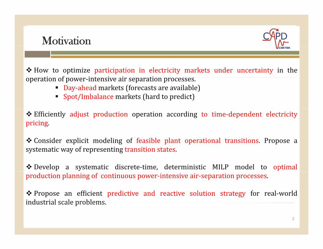
Motivation

How to optimize participation in electricity markets under uncertainty in theti f i t i i ti

How to optimize participation in electricity markets under uncertainty in theti f i t i i tioperation of power‐intensive air separation processes. Day‐ahead markets (forecasts areavailable) Spot/Imbalance markets (hard to predict)

operation of power‐intensive air separation processes. Day‐ahead markets (forecasts areavailable) Spot/Imbalance markets (hard to predict)

Efficiently adjust production operation according to time‐dependent electricitypricing.

Consider explicit modeling of feasible plant operational transitions Propose a

Efficiently adjust production operation according to time‐dependent electricitypricing.

Consider explicit modeling of feasible plant operational transitions Propose a Consider explicit modeling of feasible plant operational transitions. Propose asystematic way of representing transition states.

Develop a systematic discrete‐time, deterministic MILP model to optimal

Consider explicit modeling of feasible plant operational transitions. Propose asystematic way of representing transition states.

Develop a systematic discrete‐time, deterministic MILP model to optimalproduction planning of continuous power‐intensive air‐separation processes.

Propose an efficient predictive and reactive solution strategy for real‐worldindustrial scale problems

production planning of continuous power‐intensive air‐separation processes.

Propose an efficient predictive and reactive solution strategy for real‐worldindustrial scale problemsindustrial scale problems.industrial scale problems.

2

Problem Definition

MajorProblemMajorProblemFeaturesFeatures

Surface-treatment operations of heavy aircraft-parts are characterized by a higher complexity than typical flow-shop

Surface-treatment operations of heavy aircraft-parts are characterized by a higher complexity than typical flow-shop

1. Min/max production rates based on the plant state2. Power consumption for the different operating modes3. Power consumption follows linear correlation: PW = a + b*Production4. Min/max storage capacity in the plantcharacterized by a higher complexity than typical flow-shop

scheduling problems. This particular process in-volves a series of chemical stages

s=0,1,2,...,Li, disposed in a single production line, in which an

characterized by a higher complexity than typical flow-shop scheduling problems.

This particular process in-volves a series of chemical stages s=0,1,2,...,Li, disposed in a single production line, in which an

5. Minimum final tank levels at the end of the scheduling horizon6. Expected daily demand and hourly electricity cost.

automated material-handling tool is in charge of all transfer movements.

automated material-handling tool is in charge of all transfer movements.

StateGraphoftheStateGraphofthePlantinNetherlandsPlantinNetherlands

3

PSTN - Process State Transition Network

Plantstateswithminimumduration:Plantstateswithminimumduration:3hours3hours

RDCAP1STANDSTAND‐‐BYBY

DecompositionDecomposition in3in3 subsub‐‐states:states: 1houreach1houreach

RDCAP2

RDCB

ONONSB1 SB2

ON1 ON2 ONn

SBn

RUCB

OFFOFFON1 ON2

OFF1 OFF2

ONn

OFFn

RACAP2

RUCAP1

O

Initialsequentialtransitionstates(4)

Criticaltransitionstates(3)

Intermediatetransitionstates(8)

4

Proposed MILP Modelp

IndexesIndexes SetsSetsTime periods (168)Timeperiods(168)States(15)Days(7) Intermediatetransitionstates

Nexttotransitionstates

Initialsequentialstates

Criticaltransitionstates

EnergypricesfortheweekofJanuary152015MinTankLevelEnergypricesfortheweekofJanuary152015MinTankLevel

ParametersParametersMinproductionperhourineachstateMaxproductionperhourineachstate

VariablePowerConsumptionHourlyenergypricesfortheweek

Lastintermediateandcriticalstate

MinimumfinaltanklevelsattheendofthedayHourlyexpectedDemandFixedPowerConsumption

MinTankLevelMaxTankLevel

ContinuousVariablesContinuousVariables BinaryVariablesBinaryVariablesProductionattimetforstatesPowerconsumptionattimetI t il bl t th d f

Indicateswhetherplantoperatesinstatesduringtimeperiodt

InventoryavailableattheendoftimeperiodtObjectivefunction(totalenergycost) 5

Proposed MILP Modelp

Plant State Min/Max Storage Capacity

Sequential Transition StatesTank Level Constraints

Critical Transition States

Power Consumption

Min/Max ProductionObjective Function

6

Computational Resultsp

SOLUTIONBASEDONFLATENERGYCOSTSOLUTIONBASEDONFLATENERGYCOST Finalstatusofsolution:OPTIMALCPUtime:5.242sec.

GANTT CHART SCHEDULE TOTALCOSTTOTALCOST=40131.82=40131.82

SB

RD

RU

GANTTCHARTSCHEDULE

10

15POWERCONSUMPTION

0 20 40 60 80 100 120 140 160

ON

OFF

0

5

0 50 100 150

SOLUTIONBASEDONTIMEOFDAYPRICESSOLUTIONBASEDONTIMEOFDAYPRICES Finalstatusofsolution:OPTIMALCPUtime:0.093sec.TOTALCOSTTOTALCOST=35524.16=35524.16

RU

GANTTCHARTSCHEDULE

OFF

SB

RD

RU

5

10

15POWERCONSUMPTION

0 20 40 60 80 100 120 140 160

ON00 20 40 60 80 100 120 140 160

7

Computational Resultsp

ENERGY PRICE FORECAST (FEBRUARY 15, 2015)

PREDICTIVEMODELPREDICTIVEMODELRD

RU

GANTTCHARTSCHEDULE

( , )HOUR Monday Tuesday Wednesday Thursday Friday Saturday Sunday

1 39.99 40.88 41.87 40.22 42.88 44.48 452 36.3 36.97 39.3 37 40.02 43.32 41.353 34.48 36.2 39.8 36.82 40.11 42.03 39.274 30.38 34.19 36.67 35.38 37.7 39.6 34.955 29.21 32.29 34.33 33.38 35.14 37.1 30.356 29.49 36.03 37.32 35.51 37.06 39.41 28.49

0 20 40 60 80 100 120 140 160

ON

OFF

SB

RD

7 30.15 44.85 42.39 41.06 43.6 45.8 31.928 32.18 55.1 53.56 53.06 54.21 55.36 34.689 34.48 58.37 58.5 57.57 58.35 58.9 35.6610 38.37 60.33 60.05 60.1 59.53 58.85 41.5211 39.61 59.35 59.17 57.71 57.31 55.35 44.2212 42.67 58.77 53.31 51.82 51.17 51.5 47.3413 43.93 55.5 50.07 48 47.36 48.88 43.24

0 20 40 60 80 100 120 140 160

5

10

15POWERCONSUMPTION

14 40.03 53.26 47.57 44.98 44.65 48.13 39.9215 35.08 49.65 44.6 41.91 41.9 46.45 36.4116 33.93 46.59 43.54 41.25 41.55 44.39 33.3117 34.17 45.95 44.52 41.85 42.74 43.73 30.8918 44.36 52.91 50.84 50.07 49.96 49.49 40.4419 54.91 78.61 64.05 62.11 63.66 55.88 50.0720 56.27 72.84 58.17 59.81 60.85 55.89 43.74

0

5

0 20 40 60 80 100 120 140 160

80

90

100

175519502145

21 51.94 57.81 50.29 52.09 52.72 48.77 40.9622 44.76 51.51 42.85 45.64 46.37 45.22 36.4623 44.79 49.13 43.97 46.49 47.39 46.18 39.824 44.51 47.01 43.44 43.94 46.65 43.26 40.46

CPUtime:0.093sec.20

30

40

50

60

70

80

5857809751170136515601755

EXPECTEDEXPECTED TOTALCOSTTOTALCOST=35524.16=35524.16

REALTOTALCOSTREALTOTALCOST=41214.65=41214.650

10

20

0195390

0 20 40 60 80 100 120 140 160

INVENTORY Qmin Qmax MDTL PRODUCTION8

Computational Resultsp

PREDICTIVEMODELPREDICTIVEMODELRU EXPECTEDEXPECTED TOTAL COSTTOTAL COST = 35524 16= 35524 16

OFF

SB

RD

RU EXPECTEDEXPECTED TOTALCOSTTOTALCOST=35524.16=35524.16

BinaryVariables: 2541ContinuousVariables: 2858E ti 7730

0 20 40 60 80 100 120 140 160

ON

OFF Equations: 7730CPUtime: 0.093sec.REALTOTALCOST=41214.65

14.35%

ROLLINGROLLING‐‐HORIZONMODELHORIZONMODELRU

ScheduleChangesScheduleChanges

EXPECTEDEXPECTEDTOTALCOSTTOTALCOST=40623.78=40623.78

OFF

SB

RDBinaryVariables: 2541ContinuousVariables: 2858Equations: 7730CPU time: 0 109 sec

0 20 40 60 80 100 120 140 160

ON

CPUtime: 0.109sec.REALTOTALCOST=41326.93

9

Remarks

VeryefficientandrobustpredictiveMILP‐basedschedulingapproachModestcomputationaleffortconsideringaone‐hourtimegridandone‐weektimehorizonModelabletoconsiderallproblemfeaturesandeasytoadaptto

ti h d li ( lli h i )

INDUSTRIAL APPLICATION EXAMPLEINDUSTRIAL APPLICATION EXAMPLE

reactivescheduling(rollinghorizon)Promisingsolutionschedulingforreal‐worldAirLiquide industrialplants

Future WorkFutureWork

Evaluatedailyandhourlyreactivedecisionsbasedonenergypricechanges(dayahead market and imbalance market)aheadmarketandimbalancemarket).

TestmodelwithotherAirLiquide plantconfigurations.Identifyadditionalfeaturestobeincludedinthemodel.

Evaluatemodelwithuncertaindemands.

10