towards quantum simulation of non-abelian lattice gauge

Prepotential Framework: an overviewVariant Formulation: Simple constraint structure

Practical Implementation

Towards Quantum Simulation of Non-AbelianLattice Gauge Theories

JLab Theory Seminar

Indrakshi Raychowdhury

University of Maryland, College Park

27 January, 2020

Indrakshi Raychowdhury Towards Quantum Simulation of Non-Abelian Lattice Gauge Theories



Motivation for Quantum Computing/Simulation

Quantum computation is expected to efficiently handlethe exponential growth of information in entangledquantum systems that overwhelms classicalcomputers.

Despite of tremendous success of lattice QCDcalculations, there are some forbidden regions toexplore even with the largest supercomputers.For lattice gauge theories, quantum computers offerhope for ab initio studies of non-zero density,topological properties, and real-time phenomena,which are exponentially hard to solve classically dueto sign problems.





Quantum computation is expected to efficiently handlethe exponential growth of information in entangledquantum systems that overwhelms classicalcomputers.Despite of tremendous success of lattice QCDcalculations, there are some forbidden regions toexplore even with the largest supercomputers.

For lattice gauge theories, quantum computers offerhope for ab initio studies of non-zero density,topological properties, and real-time phenomena,which are exponentially hard to solve classically dueto sign problems.





Quantum computation is expected to efficiently handlethe exponential growth of information in entangledquantum systems that overwhelms classicalcomputers.Despite of tremendous success of lattice QCDcalculations, there are some forbidden regions toexplore even with the largest supercomputers.For lattice gauge theories, quantum computers offerhope for ab initio studies of non-zero density,topological properties, and real-time phenomena,which are exponentially hard to solve classically dueto sign problems.




State of the art

Quantum computers are still at infancy just like classicalcomputers 40 years ago.

Present day’s effort:Contructing proposals for digital and analog quantumsimulation.NISQ era computation: quantum noise.Experimental implementation in both digital and analog forsimple and/or toy models.




Quantum computation for gauge theories

Suitable Framework: Hamiltonian Lattice Gauge Theory

Schwinger model: QED in 1 + 1 dimensions

Super simple to analyze yet contains rich physicsReal time simulation of Schwinger model shows dynamicsof pair production, string breaking etc.Many analog proposals has been made in past five years.European review: arXiv:1911.00003, Davoudi et al.arXiv:1908.03210 and more.Digital computation with Schwinger model: N. Klco et al:arXiv:1803.03326 and more.First experimental realization: Martinez et al, Nature’16Many ongoing projects across the globe.




Long Term Goal: Quantum Simulating QCD

QCD: Non-abelian (SU(3)) gauge theory in 3 + 1dimensions.

Till date:ONLY A FEW ANALOG PROPOSALS

FAR FROM EXPERIMENTAL IMPLEMENTATION.ONLY ONE DIGITAL COMPUTATION(TROTTERIZATION), THAT IS TOO RESTRICTIVE [Klcoet al. arXiv: 1908.06935].WHY?






Till date:ONLY A FEW ANALOG PROPOSALSFAR FROM EXPERIMENTAL IMPLEMENTATION.

ONLY ONE DIGITAL COMPUTATION(TROTTERIZATION), THAT IS TOO RESTRICTIVE [Klcoet al. arXiv: 1908.06935].WHY?






Till date:ONLY A FEW ANALOG PROPOSALSFAR FROM EXPERIMENTAL IMPLEMENTATION.ONLY ONE DIGITAL COMPUTATION(TROTTERIZATION), THAT IS TOO RESTRICTIVE [Klcoet al. arXiv: 1908.06935].

WHY?






Till date:ONLY A FEW ANALOG PROPOSALSFAR FROM EXPERIMENTAL IMPLEMENTATION.ONLY ONE DIGITAL COMPUTATION(TROTTERIZATION), THAT IS TOO RESTRICTIVE [Klcoet al. arXiv: 1908.06935].WHY?




Drawbacks of Conventional formalism

Non-Abelian LGT : local Hamiltonian+ gauge theory Hilbertspace+ Gauss law for gauge invariance.States in the Hilbert space are predominantly unphysical,and a noisy quantum computer would get lost among them.Gauss’s law is nontrivial on a quantum computer: colorcomponents are not simultaneously diagonalizable.Different representations to be mapped onto a register ofqubits are on different footings under (and mixed by) theaction of the Hamiltonian.Crafting the action of the Hamiltonian in terms of quantumcomputer operations→ straightforward in principle butrather unnatural to do.




Alternate formulation

Prepotential formulation of LGT is developed over lastdecade starting with Mathur’05, ’07.prepotential formulation of LGT uses gauge invarianttowers of states, characterized by integer quantumnumbers.The Hamiltonian acts as a sum of ladder operators onthose towers of states, which seems far more natural forquantum computation.




1 Prepotential Framework: an overviewHamiltonian Lattice Gauge theoryIntroducing prepotentialsLoop operators and loop states

2 Variant Formulation: Simple constraint structureVirtual Point Splitting SchemePrepotential coupled to matterIn arbitrary dimension

3 Practical ImplementationSU(2) Physicality OracleTrotterizationTowards analog quantum simulation of Non-Abelian LGT




Hamiltonian Lattice Gauge theoryIntroducing prepotentialsLoop operators and loop states

Hamiltonian LGT: Variables

Discrete Spaceand Continuoustime On a link of the spatial lattice

EaR(n + i , i) = Eb

L (n, i)Rab (U(n, i))





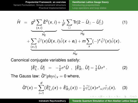
H = g2∑

(x ,i)

E2(x , i)

︸︷︷︸HE

+ 1g2

∑

�

Tr(2− U� − U†�)

︸︷︷︸HB

(1)

+∑

(x ,i)

ψ†(x)U(x , i)ψ(x + ei) + m∑

x

(−)x ψ†(x)ψ(x)

︸︷︷︸HM

.

Canonical conjugate variables satisfy:

[EaL , U] = −1

2σaU , [Ea

R , U] = 12 Uσa . (2)

The Gauss law: Ga|phys〉x = 0 where,

Ga(x) =d∑

i=1

(EaL,i(x) + Ea

R,i(x))− 12 ψ†α(x)σa

αβψβ(x), (3)





Wilson loops and Mandelstam Constraints: SU(2)

Involving two loops, each carrying one unit of flux

ONLY NON-INTERSECTING LOOPS ARE PHYSICAL





Wilson loops and Mandelstam Constraints: SU(2)

Increasing number of Loops⇒ Increasing number ofMandelstam Identities!

In prepotential formulation these fundamental Mandelstamidentities becomes local and can be analyzed as well assolved to get Orthonormal Loop states.





Prepotentials

Harmonic oscillators belonging to the fundamentalrepresentation of the gauge group defined at eachlattice site.Prepotentials transform as matter fields→ constructlocal gauge invariant variables and states from them!

Local Mandelstam constraints⇒ Exact solution isnon-trivial but possible.Prepotential formulation of SU(2), SU(3) and arbitrarySU(N) exists (ref:IR, PhD Thesis) , but we will confineourselves to SU(2) only in this talk.





SU(2) Prepotentials

Left electric fields: E aL(n, i) ≡ a†(n, i ; L)

σa

2a(n, i ; L),

Right electric fields: E aR(n + i , i) ≡ a†(n + i , i ; R)

σa

2a(n + i , i ; R).

Under SU(2) gauge transformation

a†α(L)→ a†

β(L)(Λ†

L

)βα, a†

α(R)→ a†β(R)

(Λ†

R

)βα

aα(L)→(ΛL)α

β aβ(L), aα(R)→(ΛR)α

β aβ(R).





Link Operator

From SU(2)⊗ U(1) gauge transformations of theprepotentials,

Uαβ = a†α(L) η a†

β(R) + aα(L) θ aβ(R)

Calculating the coefficients from U†U = UU† = 1,

U =1√

nL + 1

(a†

2(L) a1(L)

−a†1(L) a2(L)

)

︸︷︷︸UL

(a†

1(R) a†2(R)

a2(R) −a1(R)

)1√

nR + 1︸︷︷︸UR





Abelian Weaving, Non-abelian Intertwining and LoopStates

Link operator: Uαβ =

1√n + 1

(a†α(L) a†

β(R) + aα(L) aβ (R)

) 1√n + 1

Four basic gauge invariant operators constructed by Uαβ (n, i)Uβ

γ (n + i, j) at site (n + i) :

a†β

(i)1√

ni + 1

1√nj + 1

a†β (j) =1√ni

1√nj + 1

a†(i) · a†β (j) ≡1√

ni (nj + 1)k ij

+ ≡ Oi+ j+

a†β

(i)1√

ni + 1

1√nj + 1

aβ (j) =1√ni

1√nj + 1

a†(i) · a(j) ≡1√

ni (nj + 1)κ

ij ≡ Oi+ j−

aβ (i)1√

ni + 1

1√nj + 1

a†β (j) =1√

ni + 2

1√nj + 1

a(i) · a†(j) ≡1√

(ni + 2)(nj + 1)κ

ji ≡ Oj+ i−

aβ (i)1√

ni + 1

1√nj + 1

aβ (j) =1√

ni + 2

1√nj + 1

a(i) · a(j) ≡1√

(ni + 2)(nj + 1)k ji− ≡ O

i− j−

for i, j different directions at each site.Indrakshi Raychowdhury Towards Quantum Simulation of Non-Abelian Lattice Gauge Theories




Loop States and Linking Numbers

|{lij}〉 =∏

i 6=j

(k+)lij

lij !|0〉

Linking numbers in 2d





Mandelstam Constraints

(a†(1) · a†(2)

) (a†(1) · a†(2)

)≡(

a†(1) · a†(1)) (

a†(2) · a†(2))−(

a†(1) · a†(2)) (

a†(2) · a†(1))

Equivalent to the fundamental Mandelstam identity





Linking Numbers and Constraints

Loop State characterized by 6 linking numbers

|l12, l11, l12, l21, l22, l12〉 ≡ |{l}〉 =

(k12

+

)l12

l12!

(k11

+

)l11

l11!

(k12

+

)l12

l12!

(k21

+

)l21

l21!

(k22

+

)l22

l22!

(k 12

+

)l12

l12!|0〉 (4)

with n1 = l12 + l11 + l12 , n2 = l21 + l22 + l12 , n1 = l12 + l11 + l21 , n2 = l12 + l22 + l12

One Mandelstam constraint

k12+ k 12

+ − k12+ k21

+ + k11+ k22

+ = 0

Two U(1) Gauss Law constraints

n1(x) = n1(x + e1) & n2(x) = n2(x + e2)




Virtual Point Splitting SchemePrepotential coupled to matterIn arbitrary dimension

Motivation

In two spatial dimension, at each site there is exactly threephysical degrees of freedom.In terms of linking variables or fusion variables, identifyingthese three quantum numbers to characterize a loop stateis not straightforward.Non-linear Constraints: difficult to analyzeAn observation: dynamics on a square plaquette isidentical to the dynamics on hexagonal plaquette with onlylinear constraints (IR ’18)





Example: point splitting in 2D

Site ‘x ’ on a square lattice is virtually split into two sites‘xe & xo ’ connected by a third virtual direction 3− 3

x11

2

2

xo

xe1

1

2

2

3

3





The virtual Hexagonal Lattice

Abelian Gauss law

ni(x) = ni (x + ei)





Prepotential Formulation

Local Loop Operators

L++ij ≡ a†α(i)â†α(j) , L+−

ij ≡ a†α(i)aα(j) (5)

Above, â†α ≡ εαβa†β, âα ≡ εαβaβ, and i , j are direction indiceswith i 6= j .





Local loop state:

|l12, l23, l31〉 ≡(L++

12 )l12(L++23 )l23(L++

31 )l31

(l12 + l23 + l31)! l12! l23! l31!|0〉x , (6)





Pictorial representation of loops

Local loops on hexagonal lattice

Action on loop states





Occupation number basis

At each site x :

n1 = l12 + l31 , n2 = l12 + l23 , n3 = l23 + l31 (10)

or equivalently, l12 =12

(n1 + n2 − n3) ,

l23 =12

(n2 + n3 − n1) , (11)

l31 =12

(n1 + n3 − n2)

Abelian Gauss law

ni(x) = ni (x + ei)





Counting degrees of freedom

For x on square lattice:6 linking numbers − 2 Abelian Gauss law along twodirections − 1 Mandelstam constraint⇒ three physicaldegrees of freedom.For hexagonal lattice, two sites x1 & x2 corresponds toactual site x on the square lattice and together should haveonly three degrees of freedom.2× 3 linking numbers − 3 Abelian Gauss law⇒ 3physical degrees of freedomNo Mandelstam Constraint!





In any dimensions

For arbitrary dimension d , split each lattice site into S threepoint vertices.Total 3S number of loop states per original lattice site.d Abelian Gauss law per lattice site.S virtual sites has introduced S − 1 number of virtual linksin the lattice, each containing one Abelian Gauss lawconstraint.The number of independent loop degrees of freedom peroriginal lattice site counts to

3S − d − S + 1 ≡ 3(d − 1)

⇒ S = 2(d − 1)

where, 3(d − 1) is the physical degrees of freedom perlattice site.





In 2D, point splitting results in a hexagonal lattice.Prepotential formulation.On this hexagonal lattice, physical lattice directions arealong 1 and 2, and only the electric fields along these twodirections contribute to HE .However, in HB, the elementary loops are indeedhexagonal plaquettes.The matter field, originally at sites x of the square lattice,now lives on sites xm, which is at the middle of virtual linkalong 3.We treat the sites x ′, x ′′ on the same footing as in puregauge theory and xm to be a site of 1D lattice with matter.





Inclusion of Matter in 2d





3d lattice with matter

Matter as in 1D + pure gluonic vertices





Matter couples to gauge fields in the same way in allspatial dimention as in 1D

3

(3) follow. As required, U is an SU(2) operator-matrixon the AGL Hilbert space:

⇧AU †U⇧A = ⇧AU U†⇧A (11)

=

✓⇧A 0

0 ⇧A

◆, (12)

⇧A det(U)⇧A = ⇧A

⇣U00U11 � U01U10

⌘⇧A (13)

= ⇧A (14)

Moreover, using (8) one can show that

[U↵� , U��] = [U↵� , U†��] = 0 . (15)

In terms of prepotentials, the link operator has beenbroken into a left part UL and a right part UR, denotingthe SU(2) group to be localized at each end. In (2), thestaggered fermions, which are SU(2) doublets, also liveon lattice sites. Thus, the prepotential operators and thematter fields can all be uniquely associated with sites andthey transform in the same way; the essential di↵erencebetween matter and prepotentials is their statistics. Thisfeature enables one to easily construct all local SU(2)invariants by combining both prepotentials and matter.The invariants constructed only of the bosonic doubletsare named as local loop operators and the same con-structed combining matter with prepotentials are namedas local string operators. These local loop string oper-ators acting on the strong-coupling vacuum characterizea basis of all possible SU(2)-invariant excitations at asite. In the later parts of this work we elaborate the con-struction of this basis and its completeness. Note thatthese local loop-string states across neighbouring sites arejoined together with flux flowing along the links followingthe Abelian Gauss law (6), which is necessary to yieldthe original and non-local gauge invariant variables ofKogut-Susskind formulation—namely, the Wilson loopsand strings.

In the next section we present the local loop and stringstates in the simplest case of 1d with fundamental matter.All the essential features of coupling to matter appear in1d.

IV. LOOP-STRING FORMULATION: ONEDIMENSION

The Kogut-Susskind Hamiltonian (2) on a 1d spatiallattice reduces to

H = HE + HM (16)

Each site x of this lattice is connected to one incom-ing link along direction 1 and one outgoing link alongdirection, say, 1 as in Fig. 2. Within the prepoten-

tial framework, we attach prepotentials a†↵ (b†

↵) to thelink along the direction 1 (1). A staggered fermion field

† = ( †1,

†2) is defined on site x. The local bilinears de-

· · · · · · i o

i o

i o

FIG. 2. 1d lattice with matter, denoted by circles at the sites.

b†1

b†2

�

i x o

†

1

†2

� a†1

a†2

�

FIG. 3. A site x on a 1d lattice is associated with a fermionicdoublet { †

1, †2}. Bosonic doublets {a†

1, a†2} &{b†

1, b†2} are as-

sociated with links along 1 & 1-direction respectively origi-nating and ending at site x.

fined in Fig. 3 can couple in various ways to form SU(2)singlets. Hence, SU(2) invariance can be built into thetheory by passing from the Schwinger boson doublets toonly their SU(2)-invariant combinations. The theory willbe expressed in terms of the dynamics generated by allsuch operators.

A. SU(2)-invariant Operators: Loops, Strings andBaryons

The complete set of SU(2) invariants at site x are listedbelow.

• Hermitian number operators:

Na = a†↵a↵ (17a)

Nb = b†↵b↵ (17b)

N = †↵ ↵ (17c)

• Pure gauge operators: Loops

L++ = ✏↵�b†↵a†

� (18a)

L�� = ✏↵�b↵a� = (L++)† (18b)

L+� = b†↵a↵ (18c)

L�+ = b↵a†↵ = (L+�)† (18d)

• Gauge-Matter operators: Incoming Strings

S++in = ✏↵�b

†↵

†� (19a)

S��in = ✏↵�b↵ � = (S++

in )† (19b)

S+�in = b†

↵ ↵ (19c)

S�+in = b↵

†↵ = (S+�

in )† (19d)

• Gauge-Matter operators: Outgoing Strings

S++out = ✏↵�

†↵a†

� (20a)

S��out = ✏↵� ↵a� = (S++

out )† (20b)

S+�out = ↵a†

↵ (20c)

S�+out = †

↵a↵ = (S�+out )† (20d)

Hamiltonian

H = HE + HM

Gauss Law

Ga(x) = Eai (x) + Ea

o(x)− 12 ψ†α(x)σa

αβψβ(x), (12)





Prepotentials in 1D:

3

(3) follow. As required, U is an SU(2) operator-matrixon the AGL Hilbert space:

⇧AU †U⇧A = ⇧AU U†⇧A (11)

=

✓⇧A 0

0 ⇧A

◆, (12)

⇧A det(U)⇧A = ⇧A

⇣U00U11 � U01U10

⌘⇧A (13)

= ⇧A (14)

Moreover, using (8) one can show that

[U↵� , U��] = [U↵� , U†��] = 0 . (15)

In terms of prepotentials, the link operator has beenbroken into a left part UL and a right part UR, denotingthe SU(2) group to be localized at each end. In (2), thestaggered fermions, which are SU(2) doublets, also liveon lattice sites. Thus, the prepotential operators and thematter fields can all be uniquely associated with sites andthey transform in the same way; the essential di↵erencebetween matter and prepotentials is their statistics. Thisfeature enables one to easily construct all local SU(2)invariants by combining both prepotentials and matter.The invariants constructed only of the bosonic doubletsare named as local loop operators and the same con-structed combining matter with prepotentials are namedas local string operators. These local loop string oper-ators acting on the strong-coupling vacuum characterizea basis of all possible SU(2)-invariant excitations at asite. In the later parts of this work we elaborate the con-struction of this basis and its completeness. Note thatthese local loop-string states across neighbouring sites arejoined together with flux flowing along the links followingthe Abelian Gauss law (6), which is necessary to yieldthe original and non-local gauge invariant variables ofKogut-Susskind formulation—namely, the Wilson loopsand strings.

In the next section we present the local loop and stringstates in the simplest case of 1d with fundamental matter.All the essential features of coupling to matter appear in1d.

IV. LOOP-STRING FORMULATION: ONEDIMENSION

The Kogut-Susskind Hamiltonian (2) on a 1d spatiallattice reduces to

H = HE + HM (16)

Each site x of this lattice is connected to one incom-ing link along direction 1 and one outgoing link alongdirection, say, 1 as in Fig. 2. Within the prepoten-

tial framework, we attach prepotentials a†↵ (b†

↵) to thelink along the direction 1 (1). A staggered fermion field

† = ( †1,

†2) is defined on site x. The local bilinears de-

· · · · · · i o

i o

i o

FIG. 2. 1d lattice with matter, denoted by circles at the sites.

b†1

b†2

�

i x o

†

1

†2

� a†1

a†2

�

FIG. 3. A site x on a 1d lattice is associated with a fermionicdoublet { †

1, †2}. Bosonic doublets {a†

1, a†2} &{b†

1, b†2} are as-

sociated with links along 1 & 1-direction respectively origi-nating and ending at site x.

fined in Fig. 3 can couple in various ways to form SU(2)singlets. Hence, SU(2) invariance can be built into thetheory by passing from the Schwinger boson doublets toonly their SU(2)-invariant combinations. The theory willbe expressed in terms of the dynamics generated by allsuch operators.

A. SU(2)-invariant Operators: Loops, Strings andBaryons

The complete set of SU(2) invariants at site x are listedbelow.

• Hermitian number operators:

Na = a†↵a↵ (17a)

Nb = b†↵b↵ (17b)

N = †↵ ↵ (17c)

• Pure gauge operators: Loops

L++ = ✏↵�b†↵a†

� (18a)

L�� = ✏↵�b↵a� = (L++)† (18b)

L+� = b†↵a↵ (18c)

L�+ = b↵a†↵ = (L+�)† (18d)

• Gauge-Matter operators: Incoming Strings

S++in = ✏↵�b

†↵

†� (19a)

S��in = ✏↵�b↵ � = (S++

in )† (19b)

S+�in = b†

↵ ↵ (19c)

S�+in = b↵

†↵ = (S+�

in )† (19d)

• Gauge-Matter operators: Outgoing Strings

S++out = ✏↵�

†↵a†

� (20a)

S��out = ✏↵� ↵a� = (S++

out )† (20b)

S+�out = ↵a†

↵ (20c)

S�+out = †

↵a↵ = (S�+out )† (20d)

a†α (b†α) is attached to the link along the direction 1 (1) and astaggered fermion field ψ† = (ψ†1, ψ

†2) lives on the sites x .

Ei ,Eo and Uαβ can be rewritten using prepotentials.

Ref: Loop, String, and Hadron Dynamics in SU(2)Hamiltonian Lattice Gauge Theories, IR, Jesse Strylker,arXiv: 1912:06133.





SU(2)-invariant Operators: Loops, Strings andhadrons

Hermitian number operators:

Na = a†αaαNb = b†αbαNψ = ψ†αψα






Pure gauge operators: Loops

L++ = εαβb†αa†βL−− = εαβbαaβ = (L++)†

L+− = b†αaαL−+ = bαa†α = (L+−)†






Gauge-Matter operators: Incoming Strings

S++in = εαβb†αψ

†β

S−−in = εαβbαψβ = (S++in )†

S+−in = b†αψαS−+

in = bαψ†α = (S+−in )†






Gauge-Matter operators: Outgoing Strings

S++out = εαβψ

†αa†β

S−−out = εαβψαaβ = (S++out )†

S+−out = ψαa†αS−+

out = ψ†αaα = (S−+out )†






Pure matter operators: hadrons

B++ =12!εαβψ

†αψ†β

B−− =12!εαβψαψβ = (B++)†





This set of invariants is indeed a complete set; the bosonicoperator algebra closes

5

[·, Nb] [·, Na] [·, N ] [·, L��] [·, L�+] [·, L+�] [·, L++] [·, B++] [·, B��]

[Nb, ·] 0 0 0 �L�� L�+ +L+� +L++ 0 0[Na, ·] 0 0 0 �L�� +L�+ �L+� +L++ 0 0[N , ·] 0 0 0 0 0 0 0 2B++ �2B��

[L++, ·] �L++ �L++ 0 �Na � Nb � 2 0 0 0 0 0[L+�, ·] �L+� +L+� 0 0 Nb � Na 0 0 0 0[L�+, ·] +L�+ �L�+ 0 0 0 Na � Nb 0 0 0[L��, ·] +L�� +L�� 0 0 0 0 Na + Nb + 2 0 0

[S++in , ·] �S++

in 0 �S++in +S+�

out �S++out 0 0 0 +S+�

in

[S+�in , ·] �S+�

in 0 +S+�in �S��

out �S�+out 0 0 +S++

in 0[S�+

in , ·] +S�+in 0 �S�+

in 0 0 +S+�out +S++

out 0 �S��in

[S��in , ·] +S��

in 0 +S��in 0 0 +S��

out �S�+out �S�+

in 0

[S++out , ·] 0 �S++

out �S++out �S�+

in 0 �S++in 0 0 +S�+

out

[S�+out , ·] 0 �S�+

out +S�+out +S��

in 0 �S+�in 0 +S++

out 0[S+�

out , ·] 0 +S+�out �S+�

out 0 +S�+in 0 �S++

in 0 �S��out

[S��out , ·] 0 +S��

out +S��out 0 +S��

in 0 +S+�in �S+�

out 0

[B��, ·] 0 0 2B�� 0 0 0 0 1 � N 0[B++, ·] 0 0 �2B++ 0 0 0 0 0 N � 1

TABLE I. Commutator algebra for the Loop-String operators: divided into many subtables which summarize the algebra ofoperators at di↵erent sectors.

{·, S++in } {·, S+�

in } {·, S�+in } {·, S��

in } {·, S++out } {·, S+�

out } {·, S�+out } {·, S��

out }{S++

in , ·} 0 0 2B++ 2 + Nb � N 0 0 �L++ L+�

{S+�in , ·} 0 0 Nb + N 2B�� L++ L+� 0 0

{S�+in , ·} 2B++ Nb + N 0 0 0 0 L�+ L��

{S��in , ·} 2 + Nb � N 2B�� 0 0 L�+ �L�� 0 0

{S++out , ·} 0 L++ 0 L�+ 0 2B++ 0 2 + Na � N

{S+�out , ·} 0 L+� 0 �L�� 2B++ 0 Na + N 0

{S�+out , ·} �L++ 0 L�+ 0 0 Na + N 0 2B��

{S��out , ·} L+� 0 L�� 0 2 + Na � N 0 2B�� 0

TABLE II. Anticommutator algebra for the incoming and outgoing String operators: subdivided into four sectors.

On the AGL subspace, we can equivalently use HE =Px,i(g

2/2)E2L(x, i) =

Px,i(g

2/2)E2R(x, i).

The hopping terms from HI can be translated by look-ing at each end of a link separately. The link operatorwas given in terms of Schwinger bosons by

U(x, i) = UL(x)UR(x + ei) ,

UL(x) =1q

NL(x) + 1

✓a†2(x) a1(x)

�a†1(x) a2(x)

◆

UR(x) =

✓b†1(x) b†

2(x)

�b2(x) b1(x)

◆1q

NR(x) + 1

From this it follows that

†(x)UL(x) =1p

Na(x) + 1

�S++

out (x), S+�out (x)

�(26)

UR(x) (x) =

✓S+�

in (x)�S��

in (x)

◆1p

Nb(x) + 1(27)

Thus, the translation of a hopping term into the Loop-

String framework is

†(x)U(x, i) (x + ei) $1p

Na(x) + 1

X

�=±�S+,�

out (x)S�,�in (x + ei)⇥

1pNb(x + ei) + 1

(28)

A staggered mass term is trivially given by

(�)x †(x) · (x) = (�)xN (x). (29)

That is all there is to HM .

C. Dynamics on an orthonormal basis

Our next objective will be to describe dynamics withrespect to an orthonormal basis. The Hamiltonian hasbeen given in terms of loop and string operators, but inan orthonormal basis these operators change state nor-malization in addition to state quantum numbers. Wewill set up a basis and factorize these two behaviors be-fore describing dynamics.





The incoming and outgoing string operators are Fermionic (dueto single fermionic content) and satisfy the followinganticommutation relations

5

[·, Nb] [·, Na] [·, N ] [·, L��] [·, L�+] [·, L+�] [·, L++] [·, B++] [·, B��]

[Nb, ·] 0 0 0 �L�� L�+ +L+� +L++ 0 0[Na, ·] 0 0 0 �L�� +L�+ �L+� +L++ 0 0[N , ·] 0 0 0 0 0 0 0 2B++ �2B��

[L++, ·] �L++ �L++ 0 �Na � Nb � 2 0 0 0 0 0[L+�, ·] �L+� +L+� 0 0 Nb � Na 0 0 0 0[L�+, ·] +L�+ �L�+ 0 0 0 Na � Nb 0 0 0[L��, ·] +L�� +L�� 0 0 0 0 Na + Nb + 2 0 0

[S++in , ·] �S++

in 0 �S++in +S+�

out �S++out 0 0 0 +S+�

in

[S+�in , ·] �S+�

in 0 +S+�in �S��

out �S�+out 0 0 +S++

in 0[S�+

in , ·] +S�+in 0 �S�+

in 0 0 +S+�out +S++

out 0 �S��in

[S��in , ·] +S��

in 0 +S��in 0 0 +S��

out �S�+out �S�+

in 0

[S++out , ·] 0 �S++

out �S++out �S�+

in 0 �S++in 0 0 +S�+

out

[S�+out , ·] 0 �S�+

out +S�+out +S��

in 0 �S+�in 0 +S++

out 0[S+�

out , ·] 0 +S+�out �S+�

out 0 +S�+in 0 �S++

in 0 �S��out

[S��out , ·] 0 +S��

out +S��out 0 +S��

in 0 +S+�in �S+�

out 0

[B��, ·] 0 0 2B�� 0 0 0 0 1 � N 0[B++, ·] 0 0 �2B++ 0 0 0 0 0 N � 1

TABLE I. Commutator algebra for the Loop-String operators: divided into many subtables which summarize the algebra ofoperators at di↵erent sectors.

{·, S++in } {·, S+�

in } {·, S�+in } {·, S��

in } {·, S++out } {·, S+�

out } {·, S�+out } {·, S��

out }{S++

in , ·} 0 0 2B++ 2 + Nb � N 0 0 �L++ L+�

{S+�in , ·} 0 0 Nb + N 2B�� L++ L+� 0 0

{S�+in , ·} 2B++ Nb + N 0 0 0 0 L�+ L��

{S��in , ·} 2 + Nb � N 2B�� 0 0 L�+ �L�� 0 0

{S++out , ·} 0 L++ 0 L�+ 0 2B++ 0 2 + Na � N

{S+�out , ·} 0 L+� 0 �L�� 2B++ 0 Na + N 0

{S�+out , ·} �L++ 0 L�+ 0 0 Na + N 0 2B��

{S��out , ·} L+� 0 L�� 0 2 + Na � N 0 2B�� 0

TABLE II. Anticommutator algebra for the incoming and outgoing String operators: subdivided into four sectors.

On the AGL subspace, we can equivalently use HE =Px,i(g

2/2)E2L(x, i) =

Px,i(g

2/2)E2R(x, i).

The hopping terms from HI can be translated by look-ing at each end of a link separately. The link operatorwas given in terms of Schwinger bosons by

U(x, i) = UL(x)UR(x + ei) ,

UL(x) =1q

NL(x) + 1

✓a†2(x) a1(x)

�a†1(x) a2(x)

◆

UR(x) =

✓b†1(x) b†

2(x)

�b2(x) b1(x)

◆1q

NR(x) + 1

From this it follows that

†(x)UL(x) =1p

Na(x) + 1

�S++

out (x), S+�out (x)

�(26)

UR(x) (x) =

✓S+�

in (x)�S��

in (x)

◆1p

Nb(x) + 1(27)

Thus, the translation of a hopping term into the Loop-

String framework is

†(x)U(x, i) (x + ei) $1p

Na(x) + 1

X

�=±�S+,�

out (x)S�,�in (x + ei)⇥

1pNb(x + ei) + 1

(28)

A staggered mass term is trivially given by

(�)x †(x) · (x) = (�)xN (x). (29)

That is all there is to HM .

C. Dynamics on an orthonormal basis

Our next objective will be to describe dynamics withrespect to an orthonormal basis. The Hamiltonian hasbeen given in terms of loop and string operators, but inan orthonormal basis these operators change state nor-malization in addition to state quantum numbers. Wewill set up a basis and factorize these two behaviors be-fore describing dynamics.





Loop-String Basis States:

|nl ,ni ,no〉 =||nl ,ni ,no〉√

nl ! (nl + 1 + (ni ⊕ no))!,

where ⊕ denotes addition modulo two

||nl ,ni = 0,no = 0〉 ≡ (L++)nl |0〉||nl ,ni = 0,no = 1〉 ≡ (L++)nlS++

out |0〉||nl ,ni = 1,no = 0〉 ≡ (L++)nlS++

in |0〉||nl ,ni = 1,no = 1〉 ≡ (L++)nlB++ |0〉





||nl ,ni = 1,no = 1〉 ≡ (L++)nlB++ |0〉 , HOW?

6

1. On-site Hilbert space construction

Until this point our construction has been built on un-derlying SHO degrees of freedom, but we did not requirechoosing a basis. Now we use these tools to constructa basis in which we can explicitly express the action ofthe Hamiltonian. We start by defining “on-site” basesand afterward stitch these together to construct latticestates.

The on-site Hilbert space has three degrees of freedomcorresponding to the original occupation numbers nb, nb,and n . By themselves, these numbers are not indepen-dently SU(2)-invariant; we will construct an on-site basis|nl, ni, noi with the loop quantum number nl and quarknumbers ni, no describing strictly SU(2)-invariant exci-tations.

A basis of unnormalized kets, denoted by a double-bar|| i, can be defined as follows:

||nl, ni = 0, no = 0i ⌘ (L++)nl |0i (30a)

||nl, ni = 0, no = 1i ⌘ (L++)nlS++out |0i (30b)

||nl, ni = 1, no = 0i ⌘ (L++)nlS++in |0i (30c)

||nl, ni = 1, no = 1i ⌘ (L++)nlB++ |0i (30d)

where

ni = 0, 1 no = 0, 1 nl = 0, 1, 2, · · · , (31)

|0i is annihilated by any operator carrying at least oneminus sign, and h0|0i = 1. These states uniquely enumer-ate all SU(2)-invariant excitations that can be hosted bya site. 1 2

The norms of ||nl, ni, noi can be derived by repeateduse of the operator algebra. These types of calculationsare described in Appendix A. The result is that a nor-malized basis is given by:

|nl, ni, noi =||nl, ni, noip

nl! (nl + 1 + (ni � no))!, (37)

1 Though its utility is limited, it is straightforward to give oneunifying expression valid for all states:

||nl, ni, noi = (L++)nl [⇧00 + ⇧01 + ⇧10

�(1/2)L��⇤(S++

in )ni (S++out )no |0i ,

(32)

where

⇧00 = B��B++ , (33)

⇧01 = L�+L+� , (34)

⇧10 = L+�L�+ , (35)

and

(�1/2)L��(S++in )ni (S++

out )no |0i = �ni,1�no,1B++ |0i . (36)

2 We point out that the “baryonic” states ||nl, 1, 1i are definedon a slightly di↵erent footing. It may have seemed more naturalto introduce the states ||nl, 1, 1i as (L++)nlS++

in S++out |0i. The

problem with this follows from the fact that both string operatorsacting on the vacuum is identical to passing pure gauge flux

where � denotes addition modulo two.To describe dynamics, the SU(2)-invariant Loop-String

quantum numbers will have to be related to the non-SU(2)-invariant quantum numbers. This relationship canbe inferred from

N |nl, ni, noi = (ni + no) |nl, ni, noi , (38a)

Na |nl, ni, noi = (nl + (1 � ni)no) |nl, ni, noi , (38b)

Nb |nl, ni, noi = (nl + (1 � no)ni) |nl, ni, noi . (38c)

These imply that the following act as number operatorsin our basis:

Ni ⌘1

2(N + Nb � Na) (39a)

No ⌘ 1

2(N + Na � Nb) (39b)

Nl ⌘1

2

Na + Nb � N +

1

2

�N 2 � (Na � Nb)

2��

(39c)

Using these, (38) are promoted to operator identities tobe used in the Hamiltonian:

N = Ni + No , (40a)

Na = Nl + (1 � Ni)No , (40b)

Nb = Nl + (1 � No)Ni . (40c)

2. Operator factorization

Continuing to consider just one site, Loop-String op-erators change quantum numbers as well as state nor-malization. Now we will factor the operators in order toisolate each action.

Pertaining to the loop quantum number, we introduce“normalized” ladder operators, ⇤±:3

⇤+ ⌘ L++ 1pNl(Nl + 1) + (Ni � No) + 2

(41a)

⇤� ⌘ L�� 1pNl(Nl � 1) + (Ni � No) + 2

(41b)

through a baryon:

S++in S++

out |0i = S++in [S�+

out , B++] |0i Table I

= S++in S�+

out B++ |0i= {S++

in , S�+out }B++ |0i

= �L++B++ |0i Table II

Consequently, we would have to generalize nl to start at �1for the 11-type states only and understand (L++)�1 to mean(L++)† = L��. Instead, we choose to use one set of uncon-strained quantum numbers to capture all states uniquely.

3 We refer to an operator O as a “normalized operator” if all non-vanishing eigenvalues of O†O are unity.





Occupation number basis of prepotentials and matterto loop-string basis

Ni ≡12

(Nψ +Nb −Na)

No ≡12

(Nψ +Na −Nb)

Nl ≡12

[Na +Nb −Nψ +

12

(N 2ψ − (Na −Nb)2

)]

or equivalently,

Nψ = Ni +No ,

Na = Nl + (1−Ni)No ,

Nb = Nl + (1−No)Ni .





The Hamiltonian

HE is∑

x ,i

(g2/2)E2L (x , i) (or

∑

x ,i

(g2/2)E2R(x , i)), which in terms

of loop-string quantum number reads as

EαL (x)Eα

L (x) =

[Nl(x) + (1−Ni(x))No(x)

2

]×

[Nl(x) + (1−Ni(x))No(x)

2+ 1]

EαR (x)Eα

R (x) =

[Nl(x) + (1−No(x))Ni(x)

2

]×

[Nl(x) + (1−No(x))Ni(x)

2+ 1]





The Hamiltonian

HM = Hm + HI

Hm = m∑

x

(−)x (Ni(x) +No(x))

and

HI = ψ†(x)U(x , i)ψ(x + ei) ↔1√

Na(x) + 1

∑

σ=±σS+,σ

out (x)Sσ,−in (x + ei)1√

Nb(x + ei) + 1





Gauss Law at site x : Equivalent to U(1) theory

na(x)− nb(x) = no(x)− ni(x)





operator action (a) action (b)

–

–

–

–





operator action (a) action (b)





7

Loop-String operator factorizations

L++ = ⇤+p

Nl(Nl + 1) + (Ni � No) + 2 (46a)

L�� = ⇤�pNl(Nl � 1) + (Ni � No) + 2 (46b)

L+� = �†i �o (46c)

L�+ = ��i �†o (46d)

S++in = �†

i (⇤+)Nop

Nl + 2 � No (46e)

S��in = �i (⇤�)No

pNl + 2(1 � No) (46f)

S++out = �†

o (⇤+)Nip

Nl + 2 � Ni (46g)

S��out = �o (⇤�)Ni

pNl + 2(1 � Ni) (46h)

S�+in = ��†

o (⇤�)1�Nip

Nl + 2Ni (46i)

S+�in = ��o (⇤+)1�Ni

pNl + 1 + Ni (46j)

S+�out = �†

i (⇤�)1�Nop

Nl + 2No (46k)

S�+out = �i (⇤+)1�No

pNl + 1 + No (46l)

B++ = �†i�

†o (46m)

B�� = ��i�o (46n)

TABLE III. Factorization of all SU(2) invariant operator intocanonically-normalized fermionic modes times a loop ladderoperator times a function of number operators. The operatorexponentials are defined in (45).

The purpose of ⇤± is that their non-vanishing matrixelements in our orthonormal basis are all unity:

hn0l, n

0i, n

0o| ⇤± |nl, ni, noi = �n0

l,nl±1�n0i,ni

�n0o,no

(42)

By construction, we can trivially factorize L++ and L��

by rearranging (41a) and (41b).As for the quark quantum numbers, these are a↵ected

by the string operators and by the mixed-type loop oper-ators. We have seen that the string operators obey Fermi-like anticommutation relations, but they are not canon-ically normalized. This motivates introducing SU(2)-invariant fermionic modes �i,�o to describe them, with

{�i,�o} = {�†i ,�

†o} = 0, (43)

{�i,�†i} = {�o,�

†o} = 1 (44)

Because string operators can a↵ect loop numbers, it willprove helpful to also introduce the following shorthandoperator exponentials:

(⇤±)Nq ⌘ (1 � Nq) + ⇤±Nq (q = i, o) (45a)

(⇤±)1�Nq ⌘ ⇤±(1 � Nq) + Nq (q = i, o) (45b)

Equipped with these, all loop and string operators canbe factorized as shown in Table III. The justification forthese operator factorizations is that they realize the exact

same operator algebra. The SU(2)-invariant quark modes�i and �o will also be helpful for characterizing globalbasis states.

3. Global Hilbert space construction in one dimension

In the loop-string framework, the lattice “vacant” state|0i is characterized as that state on which

Ni(x) |0i = No(x) |0i = Nl(x) |0i = 0 for all x . (47)

It is annihilated by any L±±, S±±, or B±± carrying atleast one minus sign:

L+�(x) |0i = L�+(x) |0i = L��(x) |0i = 0 (48)

S+�in (x) |0i = S�+

in (x) |0i = S��in (x) |0i = 0 (49)

S+�out (x) |0i = S�+

out (x) |0i = S��out (x) |0i = 0 (50)

B��(x) |0i = 0 (51)

The staggered strong-coupling vacuum |⌦i or simply“vacuum” can then be defined as one with vanishing elec-tric fields and full fermion orbitals on the odd sites:

Nl |⌦i = 0

(Ni + No) |⌦i = 0 for x = 0, 2, 4, · · ·(Ni + No) |⌦i = 2 |⌦i for x = 1, 3, 5, · · ·

S±,�in (x) |⌦i = S�,±

out (x) |⌦i = 0 for x = 0, 2, 4, · · ·S±,+

in (x) |⌦i = S+,±out (x) |⌦i = 0 for x = 1, 3, 5, · · ·

For lattice basis states, matter particles are createdstarting at x = Lx � 1 down to x = 0.

|nl(0), ni(0), no(0); nl(1), ni(1), no(1); · · ·· · · ; nl(Lx � 1), ni(Lx � 1), no(Lx � 1)i (52)

For example, the (normalized) staggered strong-couplingvacuum of a four site lattice is given by

|⌦i = | 0, 0, 0; 0, 1, 1; 0, 0, 0; 0, 1, 1i= B++(1)B++(3) |0i

(53)

The ordering is most important for states with on-sitefermionic excitations. For example, a basis state describ-ing a meson string between sites x = 0 and x = 1 is givenby

|mesoni = |0, 0, 1; 0, 0, 1; 0, 0, 0; 0, 1, 1i

=1

2S++

out (0)S+�in (1) |⌦i ,

(54)

as opposed to the opposite ordering 12S+�

in (1)S++in (0) |⌦i.

Using the physical quark modes �i,�o, we can moresuccinctly characterize lattice basis states with the fol-lowing rule: Physical quarks are created from startingfrom site x = Lx � 1, working down to site x = 0, and

with �†o(x) always acting before �†

i (x).





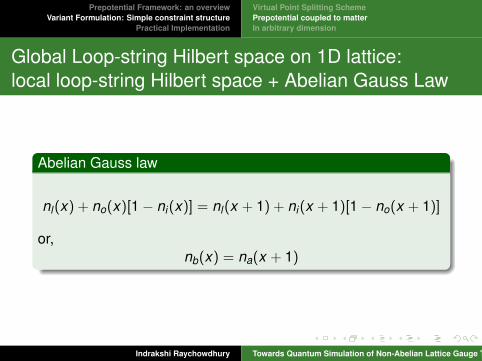
Global Loop-string Hilbert space on 1D lattice:local loop-string Hilbert space + Abelian Gauss Law

Abelian Gauss law

nl(x) + no(x)[1− ni(x)] = nl(x + 1) + ni(x + 1)[1− no(x + 1)]

or,nb(x) = na(x + 1)





Wigner-Jordan transform in one dimension

We have expressed physical matter degrees of freedom interms of the excitations of fermionic modes χi(x), χo(x) forx = 0, . . . ,Lx − 1.

These couple to each other through the hopping terms,where it is apparent that χi ’s and χo ’s are decoupled.Let us relabel the fermionic modes using Ψk fork = 0, . . . ,2Lx − 1, identifying

χi → k = 0,1, . . . ,Lx − 1 χo → Lx ,Lx + 1, . . . ,2Lx − 1

Assuming open boundary conditions, all fermioniccouplings are nearest-neighbor.All couplings can be of the form σ±k σ

∓k+1:

χ†i (x)χi(x + 1)→ −σ−x σ+x+1 , χ†o(x)χo(x + 1) → −σ−Lx +xσ

+Lx +x+1






We have expressed physical matter degrees of freedom interms of the excitations of fermionic modes χi(x), χo(x) forx = 0, . . . ,Lx − 1.These couple to each other through the hopping terms,where it is apparent that χi ’s and χo ’s are decoupled.

Let us relabel the fermionic modes using Ψk fork = 0, . . . ,2Lx − 1, identifying

χi → k = 0,1, . . . ,Lx − 1 χo → Lx ,Lx + 1, . . . ,2Lx − 1


∓k+1:


+Lx +x+1






We have expressed physical matter degrees of freedom interms of the excitations of fermionic modes χi(x), χo(x) forx = 0, . . . ,Lx − 1.These couple to each other through the hopping terms,where it is apparent that χi ’s and χo ’s are decoupled.Let us relabel the fermionic modes using Ψk fork = 0, . . . ,2Lx − 1, identifying

χi → k = 0,1, . . . ,Lx − 1 χo → Lx ,Lx + 1, . . . ,2Lx − 1


∓k+1:


+Lx +x+1







χi → k = 0,1, . . . ,Lx − 1 χo → Lx ,Lx + 1, . . . ,2Lx − 1

Assuming open boundary conditions, all fermioniccouplings are nearest-neighbor.

All couplings can be of the form σ±k σ∓k+1:


+Lx +x+1







χi → k = 0,1, . . . ,Lx − 1 χo → Lx ,Lx + 1, . . . ,2Lx − 1


∓k+1:


+Lx +x+1





Inclusion of Matter in 2d






(i) The two sites x ′, x ′′ have only loop states |l12, l23, l31〉x ′/x ′′ ,being treated identically as in pure gauge theory.(ii) The third virtual site xm along the 3− 3 direction containsboth local loop and string states |l33, s3, s3〉, being structurallyidentical to a site with matter in 1D.(iii) The Abelian Gauss laws along the three directions of thehexagonal lattice are

n1(x) = n1(x + e1), n2(x) = n2(x + e2) , (21)n3(x) + s3 = n3(x + e3) + s3 , (22)





3d lattice with matter


The modified Abelian Gauss laws on the 3D lattice are

ni(x) = ni(x + ei) , (i = 1,2,3,4,6) (23)n5(x) + s5 = n5(x + e5) + s5 . (24)





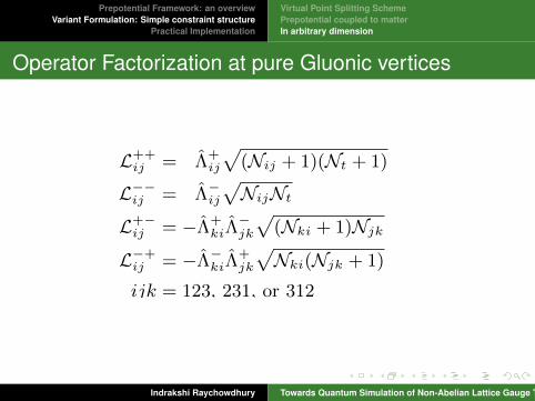
Operator Factorization at pure Gluonic vertices

17

[·, L++12 ] [·, L+�

12 ] [·, L�+12 ] [·, L��

12 ] [·, L++23 ] [·, L+�

23 ] [·, L�+23 ] [·, L��

23 ] [·, L++31 ] [·, L+�

31 ] [·, L�+31 ] [·, L��

31 ]

[L++12 , ·] 0

[L+�12 , ·] 0 0

[L�+12 , ·] 0 N2N1 0

[L��12 , ·] N1 + N2 + 2 0 0 0

[L++23 , ·] 0 L++

31 0 L+�31 0

[L+�23 , ·] 0 �L�+

31 0 L��31 0 0

[L�+23 , ·] �L++

31 0 L+�31 0 0 N3N2 0

[L��23 , ·] �L�+

31 0 �L��31 0 N2 + N3 + 2 0 0 0

[L++31 , ·] 0 0 L++

23 L�+23 0 L++

12 0 L+�12 0

[L+�31 , ·] �L++

23 L�+23 0 0 0 �L�+

12 0 L��12 0 0

[L�+31 , ·] 0 0 �L+�

23 L��23 �L++

12 0 L+�12 0 0 N1N3 0

[L��31 , ·] �L+�

23 �L��23 0 0 �L�+

12 0 �L��12 0 N3 + N1 + 2 0 0 0

TABLE V. Commutator algebra obeyed by the loop operators at a gluonic (pure gauge) vertex.

Loop operator factorizations

L++ij = ⇤+

ij

p(Nij + 1)(Nt + 1) (74a)

L��ij = ⇤�

ij

pNijNt (74b)

L+�ij = �⇤+

ki⇤�jk

p(Nki + 1)Njk (74c)

L�+ij = �⇤�

ki⇤+jk

pNki(Njk + 1) (74d)

ijk = 123, 231, or 312

TABLE VI. Factorization of all SU(2)-invariant operators ata gluonic site. Indrakshi Raychowdhury Towards Quantum Simulation of Non-Abelian Lattice Gauge Theories



SU(2) Physicality OracleTrotterizationTowards analog quantum simulation of Non-Abelian LGT

Advantages of using this framework

Non-Abelian gauge theories are now in the very samefooting as Abelian Gauge theories.

There has been several efforts in quantum simulatingSchwinger model. Many of these can be directly utilized toconstruct quantum simulator for SU(2) theory.This formalism is completely geometric and free from usingClebsch Gordon coefficients specific to SU(2), and henceis generalizable to SU(3).Constructing quantum simulator for QCD may not be so far.






Non-Abelian gauge theories are now in the very samefooting as Abelian Gauge theories.There has been several efforts in quantum simulatingSchwinger model. Many of these can be directly utilized toconstruct quantum simulator for SU(2) theory.

This formalism is completely geometric and free from usingClebsch Gordon coefficients specific to SU(2), and henceis generalizable to SU(3).Constructing quantum simulator for QCD may not be so far.






Non-Abelian gauge theories are now in the very samefooting as Abelian Gauge theories.There has been several efforts in quantum simulatingSchwinger model. Many of these can be directly utilized toconstruct quantum simulator for SU(2) theory.This formalism is completely geometric and free from usingClebsch Gordon coefficients specific to SU(2), and henceis generalizable to SU(3).

Constructing quantum simulator for QCD may not be so far.






Non-Abelian gauge theories are now in the very samefooting as Abelian Gauge theories.There has been several efforts in quantum simulatingSchwinger model. Many of these can be directly utilized toconstruct quantum simulator for SU(2) theory.This formalism is completely geometric and free from usingClebsch Gordon coefficients specific to SU(2), and henceis generalizable to SU(3).Constructing quantum simulator for QCD may not be so far.





Completed/ongoingprojects





Necassary tool for state preparation: IR, Stryker’18

We construct an oracle for checking the Abelian Gauss lawconstraints along a link.The same circuit can actually be used for all possible linksin any dimension.These routines are likely to be useful in digital simulationsbecause non-gauge invariant errors can easily arise fromthe Trotter approximation to e−itH or from quantum noise.





An analogous construction using the conventional grouprepresentation states is much less straightforward becausedifferent components of the non-Abelian Gauss lawoperator are not simultaneously diagonalizable.

The present SU(2) physicality oracle valid in any dimensionis actually simpler and cheaper than the Abelian GaussLaw Oracle (Stryker’18) for 3 (or more) dimenions.





An analogous construction using the conventional grouprepresentation states is much less straightforward becausedifferent components of the non-Abelian Gauss lawoperator are not simultaneously diagonalizable.The present SU(2) physicality oracle valid in any dimensionis actually simpler and cheaper than the Abelian GaussLaw Oracle (Stryker’18) for 3 (or more) dimenions.





Trotterization of SU(2) Hamiltonian: Work in progress

Utilizes the loop-string operators and factorization intonormalized ladder operators discussed before.Utilizes the trotterization technique for Schwinger modelHamiltonian developed in INT-ORNL collaboration, that isyet to be communicated.





In 1 spatial dimension, the loop-string-hadron model ismapped directly to a spin system and is free from anycut-off dependence with open boundary condition. Work isin progress in this direction.Comparative study of resource requirement for differentHamiltonian frameworks available in literature is underprogress.





KS to LSB: Gain in qubits

Before imposing Abelian Gauss law

∆Nq = no. of qubits required in ( KS − LSB)





Summary: some general features of this formalism

non-Abelian gauge redundancy is absent: attain a highercutoff on the physical Hilbert space than when workingwith all the redundant gauge degrees of freedom withsame number of qubits.Abelian Gauss law constraints are checked using thephysicality oracles for SU(2), in any dimension.Dynamics within infinite towers of states rather thanmultiplets of varying dimensions: natural truncationscheme lij = 2nq .Operating on towers of states more closely resembles U(1)gauge theory, so it is conceivable that other algorithmsdeveloped for Abelian theories can also be ported over toSU(2).





Summary: some general features of this formalism

Drawbacks:

point splitting technique increases the number of links tobe simulated and that plaquette operators must deal withmore links.

Hope, that this drawback is outweighed by the simpler action ofindividual link operators in a plaquette.Our construction nonetheless stands to more directly benefitfrom any progress made in algorithms for implementing U(1)plaquette operators.





T HANK YOU


towards quantum simulation of non-abelian lattice gauge

Documents