towards resilience against node failures in overlay
TRANSCRIPT

Institut fürTechnische Informatik undKommunikationsnetzeCommuni ations Systems Resear h Group
Thesis to the Semester Project
Towards Resilience Against Node Failuresin Overlay Multicast Schemes
Simon Heimlicher
Supervision: Kostas Katrinis, Prof. Dr. Bernhard Plattner
Publication: 11th August 2004
Contents
List of Figures iii
Abstract v
Preface vii
1 Introduction 11.1 Motivation . . . . . . . . . . . . . . . . . . . . . . . . . . . . . . . . . . . . . .. . . . 1
2 Background Information 32.1 Introduction to Network Protocols . . . . . . . . . . . . . . . . . .. . . . . . . . . . . 3
2.1.1 Definitions . . . . . . . . . . . . . . . . . . . . . . . . . . . . . . . . . . . .. 32.1.2 Switching . . . . . . . . . . . . . . . . . . . . . . . . . . . . . . . . . . . . .. 62.1.3 Protocol Stack . . . . . . . . . . . . . . . . . . . . . . . . . . . . . . . . .. . 62.1.4 Routing and Forwarding . . . . . . . . . . . . . . . . . . . . . . . . . .. . . . 82.1.5 TCP/IP Protocol Suite . . . . . . . . . . . . . . . . . . . . . . . . . . .. . . . 102.1.6 Communication Modes . . . . . . . . . . . . . . . . . . . . . . . . . . . .. . . 112.1.7 Multicast . . . . . . . . . . . . . . . . . . . . . . . . . . . . . . . . . . . . .. 13
2.2 Brief History of Internet Multicast . . . . . . . . . . . . . . . . .. . . . . . . . . . . . 142.3 Motivation for Overlay Multicast . . . . . . . . . . . . . . . . . . .. . . . . . . . . . . 14
2.3.1 Problems of IPv4 Multicast . . . . . . . . . . . . . . . . . . . . . . .. . . . . 152.4 Overlay Multicast Primer . . . . . . . . . . . . . . . . . . . . . . . . . .. . . . . . . . 15
2.4.1 Classification of Overlay Multicast Schemes . . . . . . . .. . . . . . . . . . . 162.4.2 Overlay Multicast Scheme Example . . . . . . . . . . . . . . . . .. . . . . . . 17
2.5 Aims and Goals of this Semester Project . . . . . . . . . . . . . . .. . . . . . . . . . . 17
3 Schemes Under Study 193.1 Scheme Classes . . . . . . . . . . . . . . . . . . . . . . . . . . . . . . . . . . .. . . . 19
3.1.1 Native IPv4 Multicast . . . . . . . . . . . . . . . . . . . . . . . . . . .. . . . 193.1.2 Host-Based Overlay Multicast . . . . . . . . . . . . . . . . . . . .. . . . . . . 203.1.3 Replicator-Based Overlay Multicast . . . . . . . . . . . . . .. . . . . . . . . . 20
3.2 Protocol Independent Multicast—Sparse Mode (PIM-SM) .. . . . . . . . . . . . . . . 213.3 Overlay Multicast Protocol (OMCP) . . . . . . . . . . . . . . . . . .. . . . . . . . . . 23
3.3.1 Contributions in OMCP . . . . . . . . . . . . . . . . . . . . . . . . . . .. . . 233.3.2 Mesh . . . . . . . . . . . . . . . . . . . . . . . . . . . . . . . . . . . . . . . . 233.3.3 Overlay Routing . . . . . . . . . . . . . . . . . . . . . . . . . . . . . . . .. . 283.3.4 Data Delivery Tree . . . . . . . . . . . . . . . . . . . . . . . . . . . . . .. . . 283.3.5 Group Dynamics . . . . . . . . . . . . . . . . . . . . . . . . . . . . . . . . .. 293.3.6 Further Improvement . . . . . . . . . . . . . . . . . . . . . . . . . . . .. . . . 29
ii

CONTENTS iii
4 Model and Evaluation Method 314.1 Methodology . . . . . . . . . . . . . . . . . . . . . . . . . . . . . . . . . . . . .. . . 31
4.1.1 Metrics . . . . . . . . . . . . . . . . . . . . . . . . . . . . . . . . . . . . . . .314.1.2 Class-based Assessment . . . . . . . . . . . . . . . . . . . . . . . . .. . . . . 344.1.3 Heuristics . . . . . . . . . . . . . . . . . . . . . . . . . . . . . . . . . . . .. . 354.1.4 Application Profiles . . . . . . . . . . . . . . . . . . . . . . . . . . . .. . . . 354.1.5 Weighting . . . . . . . . . . . . . . . . . . . . . . . . . . . . . . . . . . . . .. 36
4.2 Simulation Experiments . . . . . . . . . . . . . . . . . . . . . . . . . . .. . . . . . . . 374.2.1 Simulation Software . . . . . . . . . . . . . . . . . . . . . . . . . . . .. . . . 374.2.2 Network Topology . . . . . . . . . . . . . . . . . . . . . . . . . . . . . . .. . 374.2.3 Scenario . . . . . . . . . . . . . . . . . . . . . . . . . . . . . . . . . . . . . .. 384.2.4 Key Parameters of the Scenario . . . . . . . . . . . . . . . . . . . .. . . . . . 404.2.5 Statistical Evaluation . . . . . . . . . . . . . . . . . . . . . . . . .. . . . . . . 40
5 Results 425.1 Application Profile Results . . . . . . . . . . . . . . . . . . . . . . . .. . . . . . . . . 42
5.1.1 Variation between Runs . . . . . . . . . . . . . . . . . . . . . . . . . .. . . . 435.2 Discussion . . . . . . . . . . . . . . . . . . . . . . . . . . . . . . . . . . . . . .. . . . 43
5.2.1 Node failures . . . . . . . . . . . . . . . . . . . . . . . . . . . . . . . . . .. . 485.2.2 Obstacles . . . . . . . . . . . . . . . . . . . . . . . . . . . . . . . . . . . . .. 48
6 Conclusion 506.1 Further Research . . . . . . . . . . . . . . . . . . . . . . . . . . . . . . . . .. . . . . 50
A Conceptual Formulation 51
B Review 60
C OMCP Implementation 61C.1 Simulation Parameters . . . . . . . . . . . . . . . . . . . . . . . . . . . .. . . . . . . 61
C.1.1 Join, Leave And Death Events . . . . . . . . . . . . . . . . . . . . . .. . . . . 61C.1.2 Bootstrap Process . . . . . . . . . . . . . . . . . . . . . . . . . . . . . .. . . . 62C.1.3 Refresh Mechanism . . . . . . . . . . . . . . . . . . . . . . . . . . . . . .. . 62C.1.4 Routing Protocol . . . . . . . . . . . . . . . . . . . . . . . . . . . . . . .. . . 62C.1.5 Latency Measurement . . . . . . . . . . . . . . . . . . . . . . . . . . . .. . . 63C.1.6 Data Source Characteristics . . . . . . . . . . . . . . . . . . . . .. . . . . . . 63C.1.7 Mesh Improvement Mechanism . . . . . . . . . . . . . . . . . . . . . .. . . . 63C.1.8 Mesh Repair Mechanism . . . . . . . . . . . . . . . . . . . . . . . . . . .. . . 63C.1.9 Tree Transient Data Forwarding Characteristics . . . .. . . . . . . . . . . . . . 64
C.2 Excerpts from the OMCP Source Code . . . . . . . . . . . . . . . . . . .. . . . . . . . 64C.2.1 OMCP Node Class . . . . . . . . . . . . . . . . . . . . . . . . . . . . . . . . .64C.2.2 Member Record Class Header File . . . . . . . . . . . . . . . . . . .. . . . . . 64
Bibliography 77
Index 81
List of Figures
2.1 Ethernet link between two hosts . . . . . . . . . . . . . . . . . . . . .. . . . . . . . . 42.2 Network connected by switches . . . . . . . . . . . . . . . . . . . . . .. . . . . . . . 42.3 Internetwork connected by routers . . . . . . . . . . . . . . . . . .. . . . . . . . . . . 52.4 Message traversing the TCP/IP protocol stack . . . . . . . . .. . . . . . . . . . . . . . 72.5 Protocol stacks in hosts and routers . . . . . . . . . . . . . . . . .. . . . . . . . . . . . 82.6 Routing tables of a simple topology . . . . . . . . . . . . . . . . . .. . . . . . . . . . 92.7 Unicast communication . . . . . . . . . . . . . . . . . . . . . . . . . . . .. . . . . . . 122.8 Broadcast communication . . . . . . . . . . . . . . . . . . . . . . . . . .. . . . . . . 122.9 Multicast communication . . . . . . . . . . . . . . . . . . . . . . . . . .. . . . . . . . 132.10 Overlay multicast scheme . . . . . . . . . . . . . . . . . . . . . . . . .. . . . . . . . . 18
3.1 PIM inter-domain routing . . . . . . . . . . . . . . . . . . . . . . . . . .. . . . . . . . 213.2 PIM-SM shared tree . . . . . . . . . . . . . . . . . . . . . . . . . . . . . . . .. . . . . 223.3 Comparison between PIM-SM source-specific tree and shared tree. . . . . . . . . . . . . 23
5.1 Delay samples of three hosts . . . . . . . . . . . . . . . . . . . . . . . .. . . . . . . . 455.2 Stretch samples of three hosts . . . . . . . . . . . . . . . . . . . . . .. . . . . . . . . . 455.3 Number of data delivery tree children of four hosts . . . . .. . . . . . . . . . . . . . . 475.4 Current parent host of three hosts . . . . . . . . . . . . . . . . . . .. . . . . . . . . . . 475.5 Status of six hosts which die during the session . . . . . . . .. . . . . . . . . . . . . . 495.6 Number of packets missed at three hosts . . . . . . . . . . . . . . .. . . . . . . . . . . 49
iv

Abstract
Several emerging Internet applications require group communication. Multicast, a many-to-many communication service model for theInternet Protocol (IP), was proposed fifteenyears ago, but still lacks universal deployment. Consequently, researchers have investigatedother solutions,overlay multicastbeing the most prominent among them. In Internet termi-nology, anoverlay is a virtual network built on the IP substrate. For multicastin particular,it is usually aspanning treeformed by the hosts belonging to themulticast groupand the IPunicast links among them.
In the present semester project, a new scheme based onNarada [1] has been designedand evaluated using simulations. The primary design goal was resilience against memberfailures. Since packet forwarding is performed by ordinarygroup members, member failureleads to loss of data and consequently to quality degradation for the target application. Thenovel features of the present approach compared to Narada are overlay optimization basedon negotiation among neighbors, triggered routing updatesfor fast convergence and forcedroute changes through poisoning.
Simulation experiments have shown that in case of abrupt node failure, packet loss isunacceptably high for typical multicast applications. With forwarding entities as unreliableas personal computers,IP-level multi-pathrouting, which allows for graceful degradationon single path failure, appears to be a valuable solution.
v

vi

Preface
This work started in October 2003 and culminated with the thesis at hand in July 2004. The originalspecification of the subject was:
Overlay Multicast Simulation:Problems in the deployment of network layer multicast have led theresearch community to alternative group communication solutions. One of them is application layermulticast, where data is routed via an application layer overlay to the group members. The goal of thisthesis is to model and implement a generic simulation framework for such overlays.
This problem was then refined in the conceptual formulation1 with the title “Evaluation of RoutingSchemes for Group Communication in Packet Switched Networks.” The formulation of the problem tobe addressed was:
What is the most efficient multicast service for wide deployment in the existing Internet2 among theexisting alternatives?
The procedure to achieve this goal was planned to follow these steps: 1. Studying of related work. 2. Se-lection of a representative set of multicast schemes to put under study. 3. Discussion of the evaluationparameters and creation of application profiles. 4. Studying the use of the OMNeT++ simulator. 5. Im-plementation of the chosen protocols in the OMNeT++ environment and measurement of the variablesof interest. 6. Processing of the results and derivation of conclusions.
After the first three steps, we were planning to compare two overlay multicast schemes with IPv4multicast. However, in the process of implementing the firstoverlay multicast scheme, we noticed thatit was infeasible to implement the other two in the limited time frame of a semester project. Thus, wedecided to focus on the implementation of the first overlay multicast protocol and then compare it with anexisting implementation of the IPv4 multicast scheme. In the process of the implementation, we came upwith a few improvements over the original design. The simulation experiments with our scheme yieldedvery interesting results and we are currently in the processof putting the outcome of our work into amanuscript that we plan to submit for publication in the nearfuture.
It is our perception that the audience of semester theses is usually a very limited set of people: thesupervisor and maybe some fellow students or the parents of the author. Most theses assume a decentknowledge in the subject area and this makes them a frustrating read for people from other fields. Havingthis in mind, we tried to keep our introduction to network protocols and overlay multicast schemescomprehensible to the broad audience. Readers with diversebackground are encouraged to start theirjourney through this text with Chapter 2 on page 3 and then continue with the introduction on the nextpage. This approach should make the remaining chapters moreenjoyable.
Welcome to the world of overlay multicast!
Simon Heimlicher and Kostas Katrinis11th August 2004.
1The complete document can be found in Appendix A.2We use the termInternet with a capital ‘I’ when we talk about the global internetworkcommonly referred to as “the
Internet” that evolved fromARPAnet, developed by theAdvanced Research Projects Agency (ARPA)in the USA in the 1960s[2].
vii

viii

Chapter 1
Introduction
The growth rate of the Internet during the last decade has been spectacular. One of the key characteristicsthat enabled the transformation from an internetwork used almost exclusively by military and educationalinstitutes to the omnipresent global Internet of today is the simplicity of its underlying protocol suite,TCP/IP. At its core lies theInternet Protocol (IP),which does very little, but does it extremely well:it delivers short messages from a source machine A across allintermediate networks to a destinationmachine B.
As the Internet evolved, so did the expectations of its usersand the demands of the services runningover it. Emerging applications like audio/video streamingand conferencing, distributed computing anddatabase replication require data-intensive communication among large and heterogeneous groups ofhosts.
With the advent of broadband Internet access to the homes of more and more people, the audiencefor such data-intensive applications grows rapidly. The basic approach of replicating data packets atthe source and delivering every single copy separately is very expensive in terms of network resources.Since the connections to the end systems are getting faster at a similar pace as the servers and backbonenetworks, at some point in time, this will no longer be feasible using only unicast communication.
Clearly, a more intelligent distribution scheme is needed.
Multicast is a service model for the distribution of data from one source to a group of end systems.Even though it has been proposed fifteen years ago and today almost every router has built-in supportfor multicast forwarding, providers of rich content and value-added services still do not rely on it due toincomplete deployment.
In this chapter, we will give an overview of the currently available network layer multicast protocolsand their limitations and show where overlay multicast schemes come into play.
For readers not familiar with networking protocols and multicast, it is suggested to first readChapter 2 on page 3.
1.1 Motivation
The core network protocol of today’s Internet,IPv4 [3], offers native support for a many-to-many servicemodel termedmulticast. Unfortunately, this extension to the TCP/IP protocol suite dating back to 1988has never been adopted by its target audience, the Internet service providers. To make matters worse, sev-eral IPv4 multicast protocols exist currently. The most popular are in chronological order of occurence:Distance Vector Multicast Routing Protocol (DVMRP) [4], Multicast Open Shortest Path First (MO-SPF) [5], Core Based Trees (CBT) [6], [7], [8]andProtocol Independent Multicast (PIM) [9], [10].The next version of the IP protocol,IPv6 [11], is currently being deployed Internet-wide. This protocolversion will provide much more sophisticated multicast services from the beginning. While IPv4 mul-ticast limits the maximal number of simultaneously active groups to about220, the address range IPv6
1

2 CHAPTER 1. INTRODUCTION
reserves for multicast (about2112 addresses) should be large enough for the next few decades.Researchers have investigated other approaches in the meantime. Since increasingly deployed peer-
to-peer file sharing protocols like Gnutella [12] and BitTorrent [13] are already quite efficient even thoughthey run in the application layer on end systems, it appears feasible to also implement multicast servicesin this manner. At the time of writing, however, no protocol suite for application layer multicast has beenadopted by the IETF [14] or any other standards committee.
A considerable amount of work has been done by researchers toanalyze different approaches to themulticast problem, but a lot of questions remain unanswered. The question addressed by this thesis is:
What is themost efficientmulticast servicefor wide deployment in the existing Internet among the existing alternatives?
Our approach towards answering this question was in brief: Based on a set of requirement profiles oftypical multicast applications, we rated qualitatively most of the currently publicly available applicationlayer multicast protocols. We decided to useNarada[1], also known asEnd System Multicast (ESM)asthe basis for our simulation. We implemented Narada in theOMNeT++ [15] discrete event system simu-lator. For the generation of the Internet-like simulation topologies, we usedGT-ITM [16]. We simulateda multicast application in an Internet-like topology. Finally, we weighted the results of the simulationexperiments according to our profiles and drew conclusions about the suitability of our approach for anumber of multicast applications.
The present thesis is structured as follows. In Chapter 2, wewill present the basic concepts of net-work protocols, IPv4 multicast and introduce overlay multicast. Chapter 3 provides an overview of themulticast schemes we have considered and descriptions of the protocols we have put under study. Subse-quently, in Chapter 4, we specify our evaluation methodology and the simulated network topology. Wediscuss the results of the simulation experiments in Chapter 5 and assess the performance of our schemefor various applications. We conclude in Chapter 6.
Appendix A contains the complete initial conceptual formulation. In Appendix B, we review thegoals of the project we reached and those we haven’t achieved. Appendix C provides an explanationof the parameters of our OMCP implementation and excerpts from the C++ source code used for thesimulation in the OMNeT++ environment.

Chapter 2
Background Information
This chapter introduces the fundamental terms and conceptswe are going to touch in the thesis. We firstgive a very brief overview of network protocols and the concept of multicast communication. In Section2.2, we outline the history of multicast in the Internet. Themotivation for our work is given in Section2.3. We conclude the chapter with a primer on the core subject—Overlay Multicast—in Section 2.4.
2.1 Introduction to Network Protocols
A thorough introduction to computer networks is beyond the scope of this text. Nevertheless, we willtry to explain the essential characteristics of network protocols in this section. A broad overview of thetechnologies used at the various network layers is given in [17]. A system-oriented discussion of theimportant concepts of computer networks can be found in [18]. To keep this section brief enough, wewill take the liberty of skipping concepts that are not of prime importance to the context. The footnotesgive additional information where we omit important details.
This section is organized as follows. First, we give an overview of the concepts of computer networks,then we explain the terms relevant to the thesis in more detail.
2.1.1 Definitions
First of all, we need to give some definitions of basic components of networks we will refer to in thefuture.
Network The general termnetworkrefers to any means which allows two or more computers to com-municate with each other.
Protocol When people communicate with each other, they use a languagewhich allows them to processthe acoustic waves received by their ears or the symbols seenby their eyes. To understand each other,computers need to use a common language, too. Since we assumethat computers don’t have any intuitionin the sense that they are unable to read between the lines, computers can only communicate using a verystrict kind of language. Such languages are calledprotocols.
When discussing computer networks, a distinction between the following classes of devices is oftenmade based on their purpose.
Host A hostor end systemis either a personal computer or a server. On an abstract level, we may alsocall a host anode.
3

4 CHAPTER 2. BACKGROUND INFORMATION1 2A l i c e B o bE t h e r n e t l i n kFigure 2.1: An Ethernet link between hosts 1 and 2.1
2
A l i c e
B o bS w i t c h 1 S w i t c h 2 S w i t c h 3Figure 2.2: A simple network connected by three switches.
Link The basic building blocks for networks arelinks. A link is an abstract word for the physicalmedium that carries the signals between devices. This may bea cable or a wireless connection. Themost common medium is copper wire.Ethernet is the most popular link techonology for home andoffice networks. Ethernet uses copper wire or glass fibre or, in the wireless case, no medium at all. Tosimplify the discussion, we will assume wired networks in this section. In Figure 2.1, a simple linkbetween the computers of Alice and Bob is shown.
Switch Switches are active hardware devices which connect hosts toeach other. The resulting networkis called asubnetwork. Figure 2.2 is an example of how several hosts may be connectedto each otherusing switches. The delivery of data is performed by the switches entirely transparent to the end systemsand without a perceiveble delay.1 In contrast to routers, which will be discussed next, a switch can onlyhandle messages to hosts which are directly connected to it or another directly connected switch, i.e.,hosts in the same network.
The cloud symbol in Figure 2.2 denotes any kind of network andis commonly used to depict theInternet. It just interconnects all systems which have a connection to it.
Router Routersare active hardware devices which interconnect two or more independent networks. Anetwork of networks is termed aninternetwork.Routers are able to connect networks of different kind.
1A hub is a passive network device which has the same purpose as a switch. The difference between a hub and a switch is,that a hub only supports communication between two ports at atime. All data which are received on one port are sent out on allother ports. In contrast, a switch withn ports supports up ton
2concurrent connections at full speed in both directions. When a
switch first receives a message from a host with the physical address A, addressed at the host with physical address B, it sendsthis message on all interfaces except the one where the message came from (exactly like a hub). The switch takes note of thedestination port and the corresponding physical address. In the future, when the switch receives a message to an addressit hasalready seen, it transmits it only to the corresponding port.
2.1. INTRODUCTION TO NETWORK PROTOCOLS 5
C o m p a n yU n i v e r s i t y
A D S LP r o v i d e r
2
1 R o u t e r A R o u t e r BR o u t e r C
A l i c e
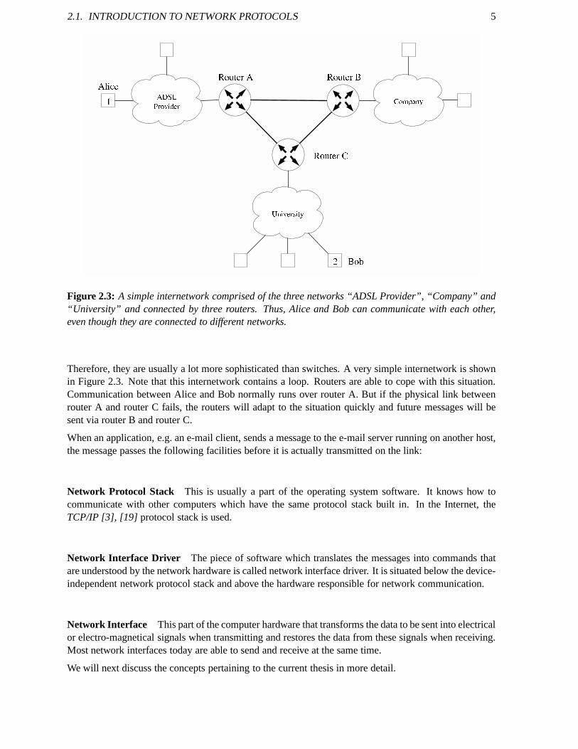
B o bFigure 2.3: A simple internetwork comprised of the three networks “ADSLProvider”, “Company” and“University” and connected by three routers. Thus, Alice and Bob can communicate with each other,even though they are connected to different networks.
Therefore, they are usually a lot more sophisticated than switches. A very simple internetwork is shownin Figure 2.3. Note that this internetwork contains a loop. Routers are able to cope with this situation.Communication between Alice and Bob normally runs over router A. But if the physical link betweenrouter A and router C fails, the routers will adapt to the situation quickly and future messages will besent via router B and router C.
When an application, e.g. an e-mail client, sends a message to the e-mail server running on another host,the message passes the following facilities before it is actually transmitted on the link:
Network Protocol Stack This is usually a part of the operating system software. It knows how tocommunicate with other computers which have the same protocol stack built in. In the Internet, theTCP/IP [3], [19] protocol stack is used.
Network Interface Driver The piece of software which translates the messages into commands thatare understood by the network hardware is called network interface driver. It is situated below the device-independent network protocol stack and above the hardware responsible for network communication.
Network Interface This part of the computer hardware that transforms the data to be sent into electricalor electro-magnetical signals when transmitting and restores the data from these signals when receiving.Most network interfaces today are able to send and receive atthe same time.
We will next discuss the concepts pertaining to the current thesis in more detail.

6 CHAPTER 2. BACKGROUND INFORMATION
2.1.2 Switching
Historically, the process of preparing the path of a messagethrough the network is calledswitching.Networks can roughly be divided into two classes by the switching strategy they use. Until the 1950s,most networks werecircuit-switched. This means, that a physical path between sender and receiver is setup for and dedicated to the connection before two hosts communicate with each other—very similar tohow telephone operators in the early days established the telephone connection on request of the caller.Once this has been accomplished, the sender may inject messages into the connection at will and no otherentity can use the physical lines involved in this connection. After all data have been sent, the connectionis torn down explicitly. No congestion can occur and all bytes of the message arrive in sequence. Circuitswitching is used in telephone networks2.
In contrast to the telephone network, current computer networks deliver data in the following way:The sender cuts the message into small pieces calledpacketsand prepares them for transmission byprepending a header indicating the destination address to every piece. The network infrastructure thenroutes these packets along potentially disjoint paths through the network to the receiver, which reassem-bles them to the original message. This type of network is called packet-switched [20],because it op-erates on individual packets. With packet switching, thereis no need to set up the path for a messagebeforehand. Instead, the first packet can be sent off as soon as it becomes available. But at no point in thetransmission is it guaranteed that the network does have enough free resources to deliver the message. Iftoo many messages are injected into the network, congestionoccurs and packets need to be buffered oreven dropped at the bottleneck. Usually this happens at a router whose input buffer is full.
Since packet-switched networks make far better use of the network resources available and allowfor greater throughput, today’s computer networks are usually packet-switched. In this text, we alwaysassume packet-switched networks.
2.1.3 Protocol Stack
There are a lot of analogies between human and computer communication. In a simple transmission ofa message from Alice to Bob, several distinct steps can be distinguished: At the beginning, Alice’s braintranslates her thought into words, for example, “Hello Bob”. Then, it sends an electrical signal to thevocal cords which orders them to generate the sound of these words. This sound wave is carried to Bob bythe physical medium, the air. His eardrums translate this mechanical wave back into an electrical signal,which can then be processed by his brain and the original thought Alice had in mind is restored. Notethat the actual message is transformed from a thought into a mechanical wave in a few steps, transmittedover the air, and then transformed back in similar steps intoa thought.
Similar transformations are applied to messages sent over anetwork by theprotocol stack3. As thename implies, we can think of it as a stack of protocols. The stages which a message passes when it istransformed are calledlayersor levels.
2Today, however, even telephone networks are mostly packet-switched. It is possible to unite the advantages of both typeswith virtual circuits: A logical connection is set up between two end points and the necessary resources are allocated for theduration of the connection.X.25 is a popular example for this kind of network. It supports permanent virtual circuits whichare an alternative for leased lines. TheAsynchronous Transfer Mode (ATM)network standard was developed to allow themultiplexing of thousands of telephone connections into one optical fibre link. It uses packet-switching to accomplishthis anda major part of the Internet backbone consists of ATM links. In Switzerland, only the last mile from the phone jack to the firstdevice of the telephone network is analog, the interconnection network is completely digital.Digital Subscriber Line (DSL)and its siblingsADSL, HDSLetc. make use of this fact.
3There exist several reference models for protocol stacks. The most popular model, at least for educational purposes, istheOSI Reference Model [21], [22], developed in 1983 by the International Organization for Standardization. OSI is an acronymfor Open System Interconnection, and this model defines a networking framework for implementing services and protocolsinseven layers. The Internet, however, uses theTCP/IPprotocol stack. We will use a combination of both models because wethink it is confusing to talk about two different models in anintroductory text.
2.1. INTRODUCTION TO NETWORK PROTOCOLS 7
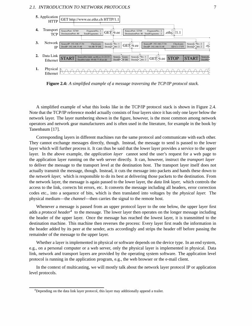
Figure 2.4: A simplified example of a message traversing the TCP/IP protocol stack.
A simplified example of what this looks like in the TCP/IP protocol stack is shown in Figure 2.4.Note that the TCP/IP reference model actually consists of four layers since it has only one layer below thenetwork layer. The layer numbering shown in the figure, however, is the most common among networkoperators and network gear manufacturers and is often used in the literature, for example in the book byTanenbaum [17].
Corresponding layers in different machines run the same protocol and communicate with each other.They cannot exchange messages directly, though. Instead, the message to send is passed to the lowerlayer which will further process it. It can thus be said that the lower layer provides a service to the upperlayer. In the above example, theapplication layer cannot send the user’s request for a web page tothe application layer running on the web server directly. Itcan, however, instruct thetransport layerto deliver the message to the transport level at the destination host. The transport layer itself does notactually transmit the message, though. Instead, it cuts themessage into packets and hands these down tothenetwork layer,which is responsible to do its best at delivering those packets to the destination. Fromthe network layer, the message is again passed to the lower layer, thedata link layer, which controls theaccess to the link, corrects bit errors, etc. It converts themessage including all headers, error correctioncodes etc., into a sequence of bits, which is then translatedinto voltages by thephysical layer. Thephysical medium—thechannel—then carries the signal to the remote host.
Whenever a message is passed from an upper protocol layer to the one below, the upper layer firstadds aprotocol header4 to the message. The lower layer then operates on the longer message includingthe header of the upper layer. Once the message has reached the lowest layer, it is transmitted to thedestination machine. This machine then reverses the process: Every layer first reads the information inthe header added by its peer at the sender, acts accordingly and strips the header off before passing theremainder of the message to the upper layer.
Whether a layer is implemented in physical or software depends on the device type. In an end system,e.g., on a personal computer or a web server, only the physical layer is implemented in physical. Datalink, network and transport layers are provided by the operating system software. The application levelprotocol is running in the application program, e.g., the web browser or the e-mail client.
In the context of multicasting, we will mostly talk about thenetwork layer protocol IP or applicationlevel protocols.
4Depending on the data link layer protocol, this layer may additionally append a trailer.
8 CHAPTER 2. BACKGROUND INFORMATION
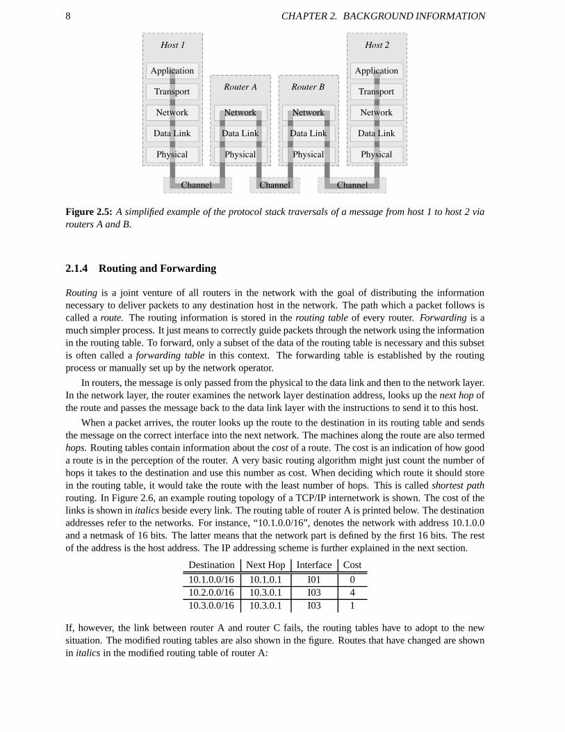
Figure 2.5: A simplified example of the protocol stack traversals of a message from host 1 to host 2 viarouters A and B.
2.1.4 Routing and Forwarding
Routing is a joint venture of all routers in the network with the goal of distributing the informationnecessary to deliver packets to any destination host in the network. The path which a packet follows iscalled aroute. The routing information is stored in therouting tableof every router.Forwarding is amuch simpler process. It just means to correctly guide packets through the network using the informationin the routing table. To forward, only a subset of the data of the routing table is necessary and this subsetis often called aforwarding tablein this context. The forwarding table is established by the routingprocess or manually set up by the network operator.
In routers, the message is only passed from the physical to the data link and then to the network layer.In the network layer, the router examines the network layer destination address, looks up thenext hopofthe route and passes the message back to the data link layer with the instructions to send it to this host.
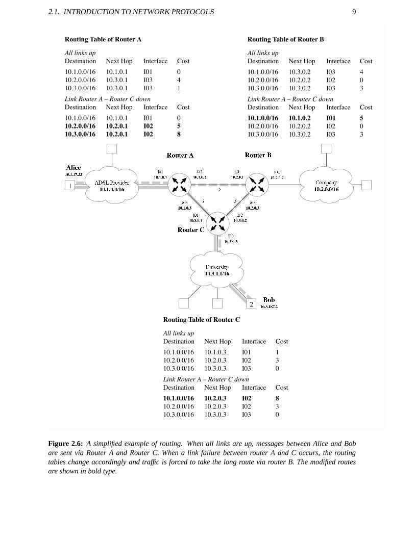
When a packet arrives, the router looks up the route to the destination in its routing table and sendsthe message on the correct interface into the next network. The machines along the route are also termedhops.Routing tables contain information about thecostof a route. The cost is an indication of how gooda route is in the perception of the router. A very basic routing algorithm might just count the number ofhops it takes to the destination and use this number as cost. When deciding which route it should storein the routing table, it would take the route with the least number of hops. This is calledshortest pathrouting. In Figure 2.6, an example routing topology of a TCP/IP internetwork is shown. The cost of thelinks is shown initalics beside every link. The routing table of router A is printed below. The destinationaddresses refer to the networks. For instance, “10.1.0.0/16”, denotes the network with address 10.1.0.0and a netmask of 16 bits. The latter means that the network part is defined by the first 16 bits. The restof the address is the host address. The IP addressing scheme is further explained in the next section.
Destination Next Hop Interface Cost
10.1.0.0/16 10.1.0.1 I01 010.2.0.0/16 10.3.0.1 I03 410.3.0.0/16 10.3.0.1 I03 1
If, however, the link between router A and router C fails, therouting tables have to adopt to the newsituation. The modified routing tables are also shown in the figure. Routes that have changed are shownin italics in the modified routing table of router A:
2.1. INTRODUCTION TO NETWORK PROTOCOLS 9
Routing Table of Router C
All links up
Destination Next Hop Interface Cost
10.1.0.0/16 10.1.0.3 I01 1
10.2.0.0/16 10.2.0.3 I02 3
10.3.0.0/16 10.3.0.3 I03 0
Link Router A – Router C down
Destination Next Hop Interface Cost
10.1.0.0/16 10.2.0.3 I02 8
10.2.0.0/16 10.2.0.3 I02 3
10.3.0.0/16 10.3.0.3 I03 0
Routing Table of Router B
All links up
Destination Next Hop Interface Cost
10.1.0.0/16 10.3.0.2 I03 4
10.2.0.0/16 10.2.0.2 I02 0
10.3.0.0/16 10.3.0.2 I03 3
Link Router A – Router C down
Destination Next Hop Interface Cost
10.1.0.0/16 10.1.0.2 I01 5
10.2.0.0/16 10.2.0.2 I02 0
10.3.0.0/16 10.3.0.2 I03 3
Routing Table of Router A
All links up
Destination Next Hop Interface Cost
10.1.0.0/16 10.1.0.1 I01 0
10.2.0.0/16 10.3.0.1 I03 4
10.3.0.0/16 10.3.0.1 I03 1
Link Router A – Router C down
Destination Next Hop Interface Cost
10.1.0.0/16 10.1.0.1 I01 0
10.2.0.0/16 10.2.0.1 I02 5
10.3.0.0/16 10.2.0.1 I02 8
I 0 31 0 . 3 . 0 . 3C o m p a n y1 0 . 2 . 0 . 0 / 1 6
U n i v e r s i t y1 0 . 3 . 0 . 0 / 1 6
A D S L P r o v i d e r1 0 . 1 . 0 . 0 / 1 6 R o u t e r A R o u t e r BR o u t e r C
A l i c e1 0 . 1 . 1 7 . 2 2
B o b1 0 . 3 . 1 8 7 . 22
1 I 0 11 0 . 1 . 0 . 1 I 0 21 0 . 1 . 0 . 2I 0 31 0 . 1 . 0 . 3I 0 11 0 . 2 . 0 . l I 0 21 0 . 2 . 0 . 2I 0 31 0 . 2 . 0 . 3I 0 11 0 . 3 . 0 . 1 I 0 21 0 . 3 . 0 . 251 3
Figure 2.6: A simplified example of routing. When all links are up, messages between Alice and Bobare sent via Router A and Router C. When a link failure betweenrouter A and C occurs, the routingtables change accordingly and traffic is forced to take the long route via router B. The modified routesare shown in bold type.

10 CHAPTER 2. BACKGROUND INFORMATION
Destination Next Hop Interface Cost
10.1.0.0/16 10.1.0.1 I01 010.2.0.0/16 10.2.0.1 I02 510.3.0.0/16 10.2.0.1 I02 8
Note, that even though on paper this routing table update looks very straightforward, it is a big challengein practice. There are many intricacies hidden in distributed algorithms. How some of them can betackled with is shown in Section 3.3.
2.1.5 TCP/IP Protocol Suite
The protocol stack run by all computers connected to the Internet is calledTCP/IP [3], [19] TCP/IPdenotes a whole protocol family. To give an overview, we follow a message traversing the TCP/IP stackand refer again to Figure 2.4.
In the application layer, we see the actual message: The sender requests a web page via the HTTPprotocol. The application layer hands this message down to the transport layer, which is running TCP.TCP cuts it into suitably large packets and prepends its header. The header indicates, which applicationlayer protocol has sent the message to allow the receiver to handle the message correctly. In TCP, thisdemultiplexing key is termed aport. The current fragment number and the total number of fragmentsis indicated as well to allow the receiver to reassemble the packets correctly, even if they don’t arrive inorder5. The message is then passed down to the IP layer, where the IP address of source and destinationhost is added.
Below the network layer, in the data link and physical layers, a variety of protocols can be used. Forhome, campus and office networks,Ethernetis the most popular protocol below TCP/IP. It can handle awide range of physical media, e.g. the IEEE 802.3 standard defines Ethernet on electrical wires or opticalfibres and IEEE 802.11 defines Ethernet for wireless devices.
We will now describe the essential protocols of the suite in more detail.
Network Layer The most important protocol of the TCP/IP suite is the network layer protocolIP.IP is an acronym forInternet protocol.The current version is IPv4, but the next version, IPv6 [11],isalready being deployed. All that IP provides is the deliveryof small messages calleddatagramsfromone host to another. This simplistic approach is largely responsible for the enormous adaptability of IPto various underlying network technologies. However, the IP protocol only offers abest-effortservice,which means that it doesn’t provide any guarantees about availability or performance of service.
Hosts communicating to each other via TCP/IP need an IP address. In the currently deployed versionof IP, version 4, addresses are 32 bit integer numbers. Conceptually, an IP address consists of twoparts6. The first part (higher order bits) forms thenetwork addressand determines to which of themany networks connected by the Internet it belongs. The restof the address is calledhost addressanddetermines to which of the hosts in the network it refers to. Where the network part ends and the host partbegins is therefore also part of the addressing informationand usually given in a bit mask callednetmask.This distinction is essential to allow routers to efficiently guide packets in large internetworks since itallows hierarchical routing. Routers outside a network need only know whether the destination host issomewhere inside the network. The delivery to the final recipient is then the responsibility of the routersinside this network. We again refer to Figure 2.6 for an example. When routing a message from host 1to host 2, router A applies the netmask with a bitwise AND to the destination address. The resulting IPaddress is then 10.3.0.0 and the router looks up the route forthis so-calledprefix. Appearently, router C
5Flow, congestion and other control data is also included, but not shown in the figure for simplicity.6Actually, there are three parts:Network, subnetworkandhostpart. But we treat the network and subnetwork part as one to
make the discussion more understandable.

2.1. INTRODUCTION TO NETWORK PROTOCOLS 11
with address 10.3.0.1 is responsible for all addresses in this network (10.3.0.1–10.3.255.255). Therefore,router A sends the message out on Interface I03. Router C thenroutes the message either directly to thesubnetwork of host 2 or to the next network, depending on whatis hidden inside the cloud.
Transport Layer Right above IP, one of the transport layer protocols, e.g.,TCPor UDP,do their duty.TCP meansTransmission Control Protocoland provides a reliable stream of data between two end pointsconnected by a network running the IP protocol. UDP stands for User Datagram Protocoland providesa very slim message delivery service which in essence makes IP datagrams accessible to applications.Consequently, UDP is not more reliable a service than IP.
Application Layer The protocols in the application layer7 provide the interface between the applica-tions and the TCP/IP stack. The most popular areHTTP, which is used by theWorld Wide WebandSMTP, which is responsible for the delivery of e-mails.
2.1.6 Communication Modes
Similar to communication among human beings who have the ability to either speak to a crowd, talk witha group or whisper into each other’s ears, computers adapt their modes of communication to their needsas well.
There are mainly three communication modes:Unicast, broadcastandmulticast.While unicast andbroadcast communication is used heavily in today’s computer networks, multicast is not in very wideuse, at least not between geographically dispersed computers. We will give possible reasons for this factin Section 2.3.
Please note that unicast communication may be uni- or bi-directional whereas broadcast and multicastcommunication is always uni-directional.
Unicast Unicast is the standard mode: One host sends a message to a single designated host. Thesender puts the address of the receiver into the destinationfield of the message header and the networkdelivers the message.
An example is shown in Figure 2.7: Host 1 sends a unicast message to host 2. This message goesfrom the sending host 3 via a switch to router A, then router D and router C. From there, it can directlyreach host 2 via the subnetwork, passing 2 switches.
Broadcast In this mode, data is emitted from one host to all other hosts.In this context, the set ofall hosts is constrained by physical or logical limits. For example, if a host connected to a switch sendsa broadcast message, only hosts connected via switches willreceive it. If a router is connected to theswitch, the router will receive the message, but not forwardit to avoid a misbehaving host to flood thewhole network. Broadcast communication is for example usedwhen host 1 needs to send a messageto host 2 in the same network, but doesn’t know the physical address of 2. The protocol responsible toresolve this dilemma is calledaddress resolution protocol (ARP)and runs in the data link layer. It workslike this: ARP sends a broadcast message asking “Who has thisIP address?” Host 2 receives this requestand sends a reply with its physical address. Host 1 now can address host 2 directly and all subsequentcommunication is unicast. Figure 2.8 shows a situation where in all three subnetworks one node issending a broadcast message. All nodes in the same broadcastdomain receive it, but routers ignorebrodcasts to ensure that one misbehaving host cannot flood the whole Internet with useless broadcastmessages.
7In contrast to the TCP/IP protocol stack, the OSI model divides the application layer into three distinct layers:session,presentationandapplicationlayer.

12 CHAPTER 2. BACKGROUND INFORMATION
12
R o u t e r A R o u t e r D R o u t e r CR o u t e r B
Figure 2.7: Unicast communication from host 1 to host 2
B
AA C CC C CA A A
B B B BBB
R o u t e r A R o u t e r D R o u t e r CR o u t e r B
Figure 2.8: Broadcast communication is confined to the broadcast domain, i.e., subnetworks A, B andC. The routers ignore broadcast messages.

2.1. INTRODUCTION TO NETWORK PROTOCOLS 13
G 4
S G 8G 6 G 7G 1 G 2 G 3 G 5
R o u t e r A R o u t e r B R o u t e r CR o u t e r D
Figure 2.9: Multicast communication from the mulitcast source hostS to all subscribers, denoted byG1..8.
2.1.7 Multicast
The idea behind multicast is to let the network deliver messages destined at a group of hosts instead ofsending a separate copy of the message to each and every receiver. Multicast communication seems tobe situated between unicast and broadcast. For multicast communication, a set of participating hostsneeds to be defined. This set is called amulticast group.When a member of this group sends, it is thesource,and all other members arereceiversor subscribers. Every multicast group needs to be assignedits owngroup addressfrom the IP multicast class D network with the address range 224.0.0.0 through239.255.255.255 as defined in [23].
In a packet-switched network with network layer support formulticast, the multicast delivery fromone host to all other hosts of the group works in the followingmanner: The source sets the destinationaddress of the message to the group address and inserts the message into the network. The network in-frastructure, i.e., the routers, then forwards the messagetowards the receivers and replicates it as needed.With network layer support for multicast, the actual delivery is completely transparent to all group mem-bers. In Figure 2.9, it is shown, how a multicast message fromthe source hostS is delivered to the groupmembers denoted byG1..8. The source host sends the message to its default gateway, router A, and thelatter then handles the delivery8. A copy is sent to routers C and D, which replicate it and send copies toall group members in their network.
The multicast service can be implemented above the network layer as well, though, and such schemesare the subject of this thesis. Multicast protocols runningabove the network layer are calledapplication-layer or overlay multicast protocolsand are introduced in Section 2.4.
8Nodes on the same subnetwork receive the multicast message via link layer multicast addressing, but this is beyond thescope of this text.
14 CHAPTER 2. BACKGROUND INFORMATION
2.2 Brief History of Internet Multicast
Multicast adddressing was defined in the IP protocol from thebeginning as a separate address range.In its early days, multicast was confined tolocal area networks (LANs),i.e., networks consisting ofend systems and hubs using Ethernet orToken Ringtechnology. Those schemes inherently supportedmulticast since all packets were available to all hosts on a network. However, extended LANs connectedthrough active devices like switches, and internetworks connected by routers were unable to delivermulticast packets.
Several proposals were published, e.g. [24], but the multicast era started only when Steve E. Deer-ing introduced multicast extensions to the existing unicast routing infrastructure in the proceedings ofthe ACM SIGCOMM ’88 conference [25], and in more detail in December 1991 in his Ph.D. thesis“Multicast Routing in a Datagram Internetwork” [26].
Deering’s work resulted in the first global multicast network, the MBone, [27], [28], a set ofmulticast-capable networks connected through IP tunnels.The routing protocol wasDistance VectorMulticast Routing Protocol (DVMRP) [4].In March 1992, the MBone was comprising about 20 hosts.In an experiment, these machines successfully received a multicast audio stream from a meeting of theInternet Engineering Task Force (IETF) [14].DVMRP assumes that most or all hosts on a multicast-enabled network wish to receive multicast traffic, thus it isconsidered adense modeprotocol. While thismay have been at least partially true for the MBone, this assumption doesn’t hold for today’s multicastgroups.
In large networks connected by routers supporting multicast in hardware, the problems of dense modemulticast need to be addressed. Currently, the most widely deployedsparse modeprotocol according to[29] is Protocol Independent Multicast (PIM-SM) [9].But even with later versions of PIM, a lot of IPv4-inherent problems remained unsolved and new challenges were introduced. The most critical open issueis the allocation of multicast addresses. IPv4 only offers aflat address space for multicast which doesn’tgive any hints as to where a multicast source or its subscribers are located. Another serious problem isthe openness of the approach. With the current popularity ofDistributed Denial of Service (DDOS) [30]attacks, the total lack of access control from traditional IPv4 multicast schemes poses a threat to all hostsin a multicast-enabled network.
The problems of address allocation and access control were recently addressed by schemes dedicatedto single-source multicast applications. Protocols of this type includeExpress [31]andSource SpecificMulticast (SSM) [32].
There are a lot of other open issues and some of them will be discussed in the next section.
2.3 Motivation for Overlay Multicast
First of all we would like to address the question why we even think about implementing multicastservices in the application layer, if they exist in the network layer as part of IPv4. Or in other words:Why did IPv4 multicast fail in that is has not been deployed Internet-wide?
There exist several lines of reasoning. One popular explanation is with the chicken and egg problem:The Internet service providers (ISPs) didn’t deploy multicast—the egg—because nobody seemed to wantto use it. The potential users—the chicken—didn’t use it because it hadn’t been deployed wide enough.
There are philosophical objections as well. The implementation of multicast services in the networklayer violates a widely accepted design paradigm summarized in the paperEnd-To-End Arguments InSystem Design[33]. Applied to multicast, it says in essence:
Since multicast services cannot be provided completely without support of the applicationlayer, they should only be implemented at a lower layer if thegain in performance is so largethat it justifies the additional cost of more complexity in the lower layer.
Another general network design paradigm is not in favour of the network layer either:

2.4. OVERLAY MULTICAST PRIMER 15
No service should be implemented in a particular layer unless this layer can completely andreliably implement the whole functionality.
One very important function that is lacking from IPv4 multicast is address management: How are mul-ticast addresses assigned and by what means are potential clients informed about the available multicastservices? A third paradigm is more specific to the network layer:
The network layer should not contain any state information.
While unicast routing has been successfully implemented inIPv4 and is doing an impressive job inrouting across a subset of the several thousandAutonomous Systems (ASs)9 comprising the Internet,the same is obviously not true for multicast. With IPv4 multicast, any router needs to potentially keepmembership information ofall hosts which are directly connected to it or to a dependent router. Thislimits the scalability when groups are dispersed among several ASs and consist of thousands of members.
While the above arguments may seem rather esoteric, there are a lot of tangible and technical prob-lems with IPv4 multicast as well. We will summarize the most prevalent in the next section.
2.3.1 Problems of IPv4 Multicast
Accounting For Internet service providers and backbone owners, multicast opens a lot of difficult ques-tions: How is the transferred data accounted for? Who pays the consumption of the precious resourcesof the routers used for multicast routing and group state information?
Interdomain Routing If a multicast group spans multiple autonomous systems, another problemarises: Since there are multiple protocols available and some ASs even offer no multicast at all, static IPtunnels need to be set up to interconnect disjoint multicastzones. This problem has lately been mitigatedby the introduction of interdomain multicast routing protocols. However, a long-term solution has yet tobe found.
Deployment Model For IPv4 multicast to fulfill its purpose, all, or close to all, hosts should be con-nected to the same multicast domain. This makes the deployment an “all or nothing” decision, and mostproviders went for nothing.
Access Control What’s more, for the streaming of copyrighted material, formulti-party games,database replication and distributed computing, IPv4 multicast often cannot be used because it providesneither authenticity nor confidentiality. Of course, the data might be encrypted at the application layerand then distributed via network layer multicast. But this would no longer be transparent to the applica-tion.
In order to work around all these problems at once, considerable effort has been put into the developmentof new multicast schemes at the application layer. Accounting, encryption, authentication—virtually allfeatures lacking from IPv4 multicast can be provided with application layer multicast. Of course, thiscomes at a price. How steep this price is we will try to at leastpartially assess with our simulationexperiments in Chapter 4.
2.4 Overlay Multicast Primer
As the term overlay implies, we are talking about a virtual network topology laid out on top of theunderlying physical network. The termapplication layer multicastdenotes a subset of schemes which are
9An autonomous system is a network or internetwork that is under the administrative control of a single entity. The termrouting domainis often used when talking about routing between ASs which isthen calledinterdomain routing.

16 CHAPTER 2. BACKGROUND INFORMATION
running in the application layer. However, the two terms areused interchangeably because all applicationlayer schemes inherently use an overlay network.
This virtual network can conceptually be divided into two structures: A redundant control topologytermedmeshand a spanning tree calleddata delivery tree. Common to all schemes is also that theyneed a central entity to bootstrap the protocol. This important machine is often calledrendez-vous point(RP).However, this is no different in IPv4 multicast. The bootstrap information in this case is the groupaddress, the distribution of which is a non-trivial problemfor which a satisfactory solution has not beenproposed yet. In overlay multicast schemes, the bootstrap information may also be offered by anotherout-of-band entity, e.g. a web site where interested recipients need to click on a link or copy and paste anaddress.
Routing in the application layer seems to be inherently lessefficient. This becomes evident whenwe take into account the overhead experienced by packets travelling through the complete protocol stackat every node. In addition, whenever a tree is used for data distribution, all nodes with more than onechild will transmit a separate copy of every data packet to every child, resulting in a manifold increaseof upstream usage. Since the upstream bandwidth of current modem and broadband connections isusually small in comparison with the ever increasing downstream capacity, this increased stress is amajor problem of overlay multicast schemes and needs to be minimized at any rate. The motivationbehind overlay multiast schemes is not to improve the performance over native IPv4 protocols but toprovide comparable performance without network infrastructure support.
2.4.1 Classification of Overlay Multicast Schemes
There exist several different classes of overlay multicastschemes. A widely accepted classificationdivides them into two main classes:Host-basedandreplicator-based.
Host-Based Host-based multicastuses only end systems to build a distribution overlay. Everynode ofthe overlay acts potentially as a router and as a data source or sink at the same time. This is in contrast toIPv4 multicast, where the whole multicast routing algorithm is running on dedicated routers, completelytransparent to the end systems.
Replicator-Based Replicator-basedmulticast needs infrastructure support in the form of dedicatedhosts capable of running the multicast routing protocol to forward and replicate the data packets dissem-inated by the source host. From the point of view of end systems, this approach is very similar to nativenetwork layer multicast.
The overlay network on which the multicast routing algorithm constructs the data delivery tree maybe established in several ways and allows to further classify the schemes according to [34].
Tree-First The most intuitive approach is calledtree-first approach. Every new node requests a list ofmembers from the rendez-vous point and subsqequently asks these members to be added to their list ofchildren. Once a node has found its parent, it tries to evaluate other nodes and if it finds one with betterproperties, it becomes its child. At the same time, it collects a list of members in its vicinity. Theseredundant nodes form the mesh and are substituted for the parent in case this host fails or the tree ispartitioned.
Schemes applying this procedure are most useful for applications where high bandwidth is moreimportant than low latency. Protocols using this approach are Yoid [35] andHMTP [36].
Mesh-First Doing the same steps the other way around works as well and this procedure is calledmesh-first approach.With this method, every node first selects a subset of the end-to-end links to form aredundant mesh connecting all end systems either among eachother, or with one or several replicators,

2.5. AIMS AND GOALS OF THIS SEMESTER PROJECT 17
depending on the scheme. Using a subset of these links, a treestructure is then dynamically created todeliver the data packets.
Protocols of this class are efficient for small multicast groups, but do not scale well beyond a fewtens of hosts. The most popular scheme of this class isNarada [1].
Implicit Performing both steps at the same time is also possible and iscalledimplicit approach.Here,the nodes are usually arranged in clusters and the optimization works towards putting the nearest neigh-bors in the same cluster, while respecting upper and lower bounds of cluster size.
The advantage of this approach is its flexibility and scalability. NICE [37], CAN-Multicast [38]andScribe [39]are popular representatives of this class.
2.4.2 Overlay Multicast Scheme Example
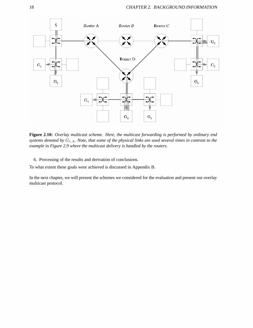
In Figure 2.10, an example of an overlay network is shown. Thethick grey denote end-to-end connectionswhich form part of the overlay network. These logical connections do not correspond to the physical linksof the underlying network. Rather, they are virtual connections between end systems. In this example,hostS is the multicast source and all hosts marked withG1..8 are subscribers.
In the leftmost network, the two group membersG1 andG2 can be reached by the sourceS usingdirect overlay links because they are in the same physical network. The receivers in the bottom networkare connected to the source via the overlay link fromS to G4, which passes routersA andD. FromG4,data packets are delivered to hostsG3 andG5 via direct overlay links. The hosts in the rightmost networkare attached to hostG4 via an overlay link passing routersD andC. From hostG8, data is delivered tohostsG6 andG7.
Note that in this example the physical link from routerD to hostG4 is used twice for every datapacket. The physical link from hostG4 to its switch is even passed by four copies of the same packet.This inefficiency is unavoidable because the overlay network is constructed without information aboutthe physical topology. The overlay routing algorithm can measure certain properties of links, e.g. theroundtrip time of a packet, but it cannot determine the exacttopology. Thus, every overlay network isinherently less efficient than the underlying physical network.
2.5 Aims and Goals of this Semester Project
The subject of the conceptual formulation for this semesterproject is
One approach to provide multicast services is application layer multicast, where data is routedvia an application layer overlay to the group members. The goal of this thesis is to model andimplement a generic simulation framework for such overlays.
The complete document can be found in Appendix A. The question to be addressed is
What is the most efficient multicast service for wide deployment in the existing Internet amongthe existing alternatives?
The procedure should follow these steps:
1. Study of related work.
2. Selection of a representative set of multicast schemes toput under study.
3. Discussion of the evaluation parameters and creation of application profiles.
4. Study the use of the OMNeT++ simulator.
5. Implementation of the chosen protocols in the OMNeT++ environment and measurement of thevariables of interest.
18 CHAPTER 2. BACKGROUND INFORMATION
G 4
S G 8G 6 G 7G 1 G 2 G 3 G 5
R o u t e r A R o u t e r B R o u t e r CR o u t e r D
Figure 2.10: Overlay multicast scheme. Here, the multicast forwarding is performed by ordinary endsystems denoted byG1..8. Note, that some of the physical links are used several timesin contrast to theexample in Figure 2.9 where the multicast delivery is handled by the routers.
6. Processing of the results and derivation of conclusions.
To what extent these goals were achieved is discussed in Appendix B.
In the next chapter, we will present the schemes we considered for the evaluation and present our overlaymulticast protocol.

Chapter 3
Schemes Under Study
This chapter discusses our selection of schemes to evaluateand a description of our custom overlaymulticast protocol.
3.1 Scheme Classes
3.1.1 Native IPv4 Multicast
We have analyzed the most popular multicast protocols for IPv4. We rated them qualitatively against thefollowing criteria: Current deployment status, flexibility and suitability for future Internet-wide deploy-ment.
DVMRP The first multicast protocol proposed for TCP/IP networks in1988 was theDistance VectorMulticast Routing Protocol (DVMRP) [4]. It is a multicast extension to the unicast distance vectorrouting protocolRouting Information Protocol (RIP) [40], [41],but it builds its own multicast routingtable based on which it constructs areverse path forwardingtree. When DVMRP was developed, itwas assumed that almost everybody in a network would want to subscribe to a multicast group and it isaccordingly termed adense modeprotocol. Data destined at multicast groups are sent to the designatedDVMRP routers of all subnetworks in a DVMRP-enabled domain.If there are no multicast subscribersin a certain subnetwork, its designated router may ask its upstream router to be pruned from the tree.Both routers store this information for a few minutes and then a new prune message needs to be sent bythe downstream router. This costs potentially a lot of memory in routers which are connected to manynetworks with no subscribers. Obviously, this approach does not scale well. Additionally, the maximaldiameter of a DVMRP multicast group is limited to 32 links. Toremedy this limitation, a hierarchicalmodel was proposed in 1995 [42] to increase the scalability,but it was not blessed with long standingsuccess.
DVMRP failed our examination because it is depending on one particular unicast routing protocoland does not appear to be scalable enough for the Internet of today.
MOSPF The unicast routing protocol that mainly replaced RIP was the link-state routing protocolOpen Shortest Path First (OSPF) [43], [44].Based on this, theMulticast Open Shortest Path First(MOSPF) [5] scheme was proposed in 1994. For multicast, the link-state updates are extended bygroup membership information. This allows all routers in a routing domain to draw a complete, up-to-date image of the topology and group membership. When a multicast data packet arrives at a router,this device computes a shortest-pathsource-specific treerooted at the subnetwork of the sender. Ifthis calculation shows that the router forms part of this tree, it forwards the packet accordingly. Thecomputation of the shortest-path using Dijkstra’s algorithm, however, is computationally involved and
19

20 CHAPTER 3. SCHEMES UNDER STUDY
the distribution of the link-state packets relies on a reliable broadcasting mechanism calledflooding,which is not scalable for wide area networks like the Internet.
MOSPF thus failed also because it relies on a specific unicastrouting protocol and due to strongconcerns regarding its scalability.
PIM We have chosenProtocol Independent Multicast (PIM) [9], [10].as a representative protocol forIPv4-based multicast. PIM offers high flexibility as it provides two different modes of operation: Forsessions with high node density, it may be run in dense mode (PIM-DM), whereas if density is low, itcan be run insparse mode(PIM-SM). PIM-DM uses ashared tree,i.e., the data delivery tree is rootedat one router and is the same for all source hosts. PIM-SM starts with a shared tree as well but has theability to switch to a source-specific tree later on if this seems useful.
PIM appears to be the most widely-deployed IPv4 multicast protocol, according to for example [29].To make the comparison as fair as possible, we considered only PIM-SM, because most overlay multicastschemes are targeted at sparse groups. Unfortunately, we did not have enough time to run simulationexperiments with this protocol, but it will be discussed in detail in Section 3.2.
CBT Focused on scalability from the very beginning was the schemeCore Based Trees (CBT) [6], [7],asparse modeprotocol. It uses the same root node termedcorefor all sources and uses a more complexalgorithm to construct a shared tree than PIM-SM.
CBT version 1 did not have much success, the incompatible version 2 is not widely deployed eitherand version 3 is currently an expired Internet-draft [8]. CBT was thus disregarded because of lackingdeployment.
3.1.2 Host-Based Overlay Multicast
In this area, we have looked atYoid [35] andEnd System Multicast (ESM)[1].
ESM The routing protocol of the ESM scheme,Narada,is quite sophisticated and seems to make gooduse of the processing power offered in today’s end systems. We decided to take this scheme as a basisand design and implement a custom architecture for our measurements. For easier reference, we will callour schemeOverlay Multicast Protocolor OMCP . It will be specified in detail in Section 3.3 on page23.
Yoid This scheme is host-based in its basic mode, but its performance may be enhanced by the in-stallation of dedicated replicators at critical points in the Internet. Yoid uses a tree-first approach withclustering. A new member gets a number of currently active group members and asks the most suit-able to be its parent. Since Yoid is not specifically designedto support classical multicast applicationslike streaming but also employs caching for file transfers, we decided to use the more generally-scopedNarada.
3.1.3 Replicator-Based Overlay Multicast
We evaluatedALMI [45], OMNI [46], Overcast [47],andScattercast [48].Our qualitative examinationof the above protocols led us to choose OMNI. ALMI uses a completely centralized approach, whichsets it very far apart from the distributed nature of the other two candidates. The application-specificextensions of Overcast and Scattercast made the comparisonwith network layer multicast appear ques-tionable. The goal of OMNI, on the other hand, is a minimal latency distribution tree using dedicatedreplicator nodes.

3.2. PROTOCOL INDEPENDENT MULTICAST—SPARSE MODE (PIM-SM) 21L e g e n d I G M P c o n n e c t i o nP I M c o n n e c t i o nI n t e r d o m a i n l i n kP I M D o m a i nP I MR o u t e r P I MR o u t e rP I MB o o t s t r a pR o u t e r P I MB o r d e rR o u t e r
P I M D o m a i nP I MB o r d e rR o u t e rN o n $ P I M $ e n a b l e dD o m a i nB o r d e rR o u t e rP I MR o u t e r
P I M D o m a i nP I MB o r d e rR o u t e rB o r d e rR o u t e rH o s t
H o s tH o s t
Figure 3.1: Example internetwork topology to show how PIM operates across non-PIM-enabled do-mains
3.2 Protocol Independent Multicast—Sparse Mode (PIM-SM)
PIM-SM version 1 is described in RFC 2362, published in June 1998 [9]. The most recent develop-ment was the submission of the latest PIM-SM version 2 specification to the IESG in April 2004 forconsideration as a proposed standard.
All mentioned IPv4 multicast protocols rely on theInternet Group Management Protocol (IGMP)[49] to manage communication between end systems and their localmulticast router. Hosts can join andleave groups by sending their router anIGMP Joinor anIGMP Leavemessage, respectively. All hostswhich have registered their membership in a group with a certain group address are then forwarded allpackets destined to this address by the router.
PIM conceptually divides networks into PIM domains, i.e., areas with PIM support, and all otherareas without support for PIM. Thus, the task of PIM is on the one hand to distribute data within PIMdomains and on the other hand to provide for unicast connections using interdomain routing to connectthese islands. An example of this architecture is shown in Figure 3.1.
The first IPv4 multicast protocol, DVMRP, assumed that all hosts in a network were group membersand constructed a tree comprising all hosts. It then pruned branches where no group members wereavailable. PIM-SM uses the opposite concept: It assumes, that no group members exist. Therefore,group subscribers need to send anexplicit join packet to the rendez-vous point in order to start receivingdata sent to the group. Group members need to check periodically whether they receive data. It is thisexplicit join model that makes PIM-SM so much more scalable than dense mode multicast protocols likeDVMRP and MOSPF.
Another important difference is that PIM-SM uses a single tree to distribute data to all PIM routerswith active group members. This tree is rooted at a well-defined machine calledrendez-vous point (RP).This is in contrast to thesource-specific treemodel used by DVMRP where a source-specific tree ismaintained for every group member that has sent some data recently. This increases the scalabilitytremendously. But using a single tree is not necessarily optimal for all sources in terms of latency, as we

22 CHAPTER 3. SCHEMES UNDER STUDY
R e n d e z �v o u sP o i n t S o u r c eP I MR o u t e r
R e c e i v e rP I MR o u t e rP I MR o u t e r R e c e i v e rP I MR o u t e rR e c e i v e r P I MR o u t e rR e c e i v e r R e c e i v e r
Figure 3.2: PIM-SM shared tree. The shared tree is always available in PM-SM. The multicast sourcesends the data to the rendez-vous point, and from there, the delivery is performed along the same tree,independent of the source host. Note that all data packets from the source cross the rendez-vous point.(Border routers are omitted in the figure for simplicity.)
will see later in an example. The selection of an optimal rendez-vous point is an NP-complete problemand is in all practical implementations approximated usingheuristics.
All PIM routers who need to receive data for a certain group register their group membership at therendez-vous point of this group. A rendez-vous point may serve several groups and every group of aparticular domain uses only one RP. Information about RPs isdistributed bybootstrap routerswithin aPIM domain. Every physical network needs at least one PIM router. This machine constantly collectsinformation about rendez-vous points. PIM domains are connected viamulticast boundary routerswhichserve as gateways and transmit information about rendez-vous points to the PIM domain at the otherend. Every PIM router with active subscribers periodicallysends a PIM Join data unit to the rendez-vouspoint to indicate that it still needs the packets for this group. The join process in a PIM domain works asfollows:
1. The joining host sends an IGMP Join message to the designated router of its subnetwork.
2. The designated router searches its records about rendez-vous points for the responsible RP. Obvi-ously, for this to be successful, the router needs to have received this information from a bootstraprouter beforehand.
3. Multicast data packets sent from the source to the rendez-vous point are replicated at the RP andforwarded to all PIM domains with active group members. The border routers of these domainsthen forward data along the distribution tree to all PIM routers inside the domain which have sent aPIM Join message recently enough.
To put away with the inefficiency of a shared tree, PIM-SM establishes a source-specific tree once thedata rate of a source exceeds a certain threshold. A comparison between a shared tree (dashed lines)and the corresponding source-specific tree is shown in Figure 3.2. The process that leads to such a treeis complex and beyond the scope of this text. It is remarkable, however, that this tree is established assoft state, which means that it is destroyed if the forwarding state has not been renewed during a given

3.3. OVERLAY MULTICAST PROTOCOL (OMCP) 23
R e n d e z �v o u sP o i n t S o u r c eP I MR o u t e r
R e c e i v e rP I MR o u t e rP I MR o u t e r R e c e i v e rP I MR o u t e rR e c e i v e r P I MR o u t e rR e c e i v e r R e c e i v e r
Figure 3.3: PIM-SM source-specific tree. Such a tree is only establishedonce the data rate of a sourcehas exceeded a certain threshold. Note that this tree doesnot involve the rendez-vous point. The sharedtree is drawn with dashed lines for comparison. (Border routers are omitted in the figure for simplicity.)
timeout interval. This simplifies the protocol, but can leadto a high amount of control traffic, especiallyif large networks are involved, because receivers will try to keep their trees established even if no dataare sent for an arbitrary period of time.
3.3 Overlay Multicast Protocol (OMCP)
In this section, we will describe Narada and point out what wehave done differently in our custom pro-tocol termedOMCPfor easier reference. The scheme currently works towards minimizing the perceivedoverlay latency, but other metrics could also be used as longas they are attainable by end systems.
3.3.1 Contributions in OMCP
There are a number of differences between OMCP and Narada. Wewill explain them in detail in thedescription in the next sections, but here is a list of the most notable contributions:
• Negotiated improvement of the mesh overlay structure.
• Route poisoning to control the data delivery tree.
• Triggered routing updates for faster routing convergence.
• Faster incorporation of fresh members into the data delivery tree.
• More accurate measurement of link latency.
3.3.2 Mesh
Since Narada is a mesh-first approach, its performance is governed mainly by the quality of the mesh. Asophisticated mesh setup and improvement strategy is thus vital to the success of the whole scheme. The

24 CHAPTER 3. SCHEMES UNDER STUDY
mesh improvement should be based on the metric which is most critical for the application because thedata delivery tree can at most perform as good as the mesh.
Mesh Establishment And Maintenance
The evolution of the mesh is not described in the Narada paper. In OMCP, nodes strive very fast towardstheir minimal degree and then become more selective about which links they add. It is therefore wise notto choose too high a minimal degree parameter, i.e., no greater than about five, to avoid adding lots ofunderperforming links which will be dropped later. Here is ashort breakdown of how a multicast groupevolves:
1. A node decides to initiate a group and makes the group address available to other potential mem-bers. A well-defined rendez-vous point could be put into service and keep track of active groupsand provide a partial list of active members. Or there might be a web page, where groups andmembers can be registered and retrieved by new users.
2. To join the mesh, a node sends anAddMeshLinkmessage to one or more active group members.The recipients will then decide based on their current number of mesh links if they can take onemore mesh link. If yes, they send an affirmative reply and the mesh link is established. If not, a listof active members is sent back and the node chooses another member.
As soon as a node has established the first mesh link, it startsexchanging the following messages withits mesh neighbors:
• Refresh messages:These contain a list of all known group members and a sequencenumber forevery member. If a node stops receiving refresh messages with increasing sequence number froma certain member, it assumes either the member to be dead or the mesh to be partitioned and startsthe probing mechanism (see below).
• Routing updates:With these packets, mesh neighbors exchange their completerouting tables. Theroute entries contain the next hop address, the associated latency and the complete path to thedestination. Routing updates are sent periodically. Additionally, an update is triggered wheneverchanges to the routing table occur and no RoutingUpdate is scheduled within a very short time-frame.
• Pings: Similar to ICMP echo requests1, these messages request an echo message and are used tomeasure the latency of links. Depending on the application,those packets might be enlarged usingpadding to get more accurate measurements, e.g. for downloads of large files. Periodically, everymember sends Pings to every member to make sure it has recent enough latency measurements.
• Routing update requests:Similar to Pings, this kind of message asks the receiver to reply with itscomplete routing table. The sender then uses this information to calculate if a mesh link should beadded.
Mesh Performance Measurement
Only on the basis of recent and accurate latency measurements is it possible to improve the mesh con-stantly and to reliably find better links. In the specification of Narada, it is just mentioned that membersperiodically probe each other to measure the unicast latency.
Narada uses the same kind of messages for the measurement of unicast links and to check if a memberis dead and requires the receiver to respond to these messages with its complete routing table. Since thesize of the routing table may vary depending on the age of a node and the number of members in the
1Internet Control Message Protocol (ICMP)is a companion protocol to IP and is used for the communication betweenrouters and end systems.Echo Requestmessages are mostly used to check if a host is running or to measure the roundtripdelay.

3.3. OVERLAY MULTICAST PROTOCOL (OMCP) 25
group, affecting directly the processing time at the receiver as well as the transmission time of the reply,we introduced three different packet types. Ping packets are used to measure the performance and maybe of arbitrary length. It might be advisable to adapt the length of the Ping messages to the length of datamessages. The second packet type is calledProbeand is used solely to determine if a member is dead.The third kind is termedRoutingRequestand asks the receiver to send back its complete routing table.
We developed the following measurement mechanism for OMCP:Whenever a node is informedabout a new member, it waits for a random time bounded by a parameter value and then sends the firstPing message to the new member. This random delay is essential to avoid that members which havejust come online are flooded with Pings by all current group members. In steady-state, every node sendsPings to group members periodically. In Narada, the target is selected randomly. We think that this canbe dangerous because the law of great numbers does not necessarily apply for groups with a few dozensof members. A node might send Pings unevenly distributed over all group members and thus never getlatency information about potentially very fast links.
Our approach calculates the interval between two Pings to the same host,Tping, with respect to atime parameterTpingTarget as follows:
Tping =TpingTarget
N,
whereN is the number of group members that the host is aware of.
EveryTping seconds, an OMCP node does the following: It searches for themember record that has theoldest Ping time stamp, sends a Ping to this member and updates the Ping time stamp in the memberrecord.
Under steady-state conditions, this approach guarantees,that a Ping message is sent to every groupmember in an interval ofTpingTarget. Thus, the latency measurement of no link grows older thanTpingTarget and all group members are sent Pings in equal intervals.
The links to mesh neighbors are evaluated more frequently. This allows to detect almost immediatelywhen a mesh link goes down and to replace it.
Mesh Improvement
The Narada paper gives a description of the procedure to evaluate if a new link should be added or acurrent one be dropped. The scheduling algorithm for the evaluation, however, is not specified. So wecame up with the following approach in OMCP: Every node alternates between evaluating its currentmesh links and checking out new links. If it decides to add or drop a mesh link, it subsequently waits forsome time before running the next evaluation cycle to allow the routing to converge. For similar reasons,a fresh link is granted a grace period, during which it cannotbe dropped.
Mesh Reduction Based on its own routing table and the stored routing tables of all known members,every node periodically calculates a value calledconsensus costfor every mesh link. The consensus costof a link indicates, what the cost is of dropping this link in the view of the hosts at both ends. First, thenodes at both ends count, how many of their routes use the other host as first hop. This number is the costfrom their point of view. The consensus cost is defined as the maximum of both these numbers. Howthis value is computed in OMCP is described later in this section.
It is not clearly defined whether Narada evaluates all links or only links with certain characteristics.In our protocol, we evaluate links with the following properties:
• The link is active.

26 CHAPTER 3. SCHEMES UNDER STUDY
• The link is not in use by the data delivery tree.
• The grace period of the link is over.
• The latency measurement and the stored routing table of the member at the other end are recentenough.
• The link latency is greater than a minimum parameter.
As specified in Narada, member A calculates the consensus cost to mesh neighbor B as follows: It countsthe number of routes in its routing table that use B as first hopand stores this value. It then calculates thecost of dropping the link from member B’s point of view using its stored routing tables in the memberrecord and stores this value as well. The consensus cost is obtained as the maximum of both costs.
After the consensus costs have been calculated, the lowest cost link is dropped if and only if the costis below the currentcost threshold.This value depends on the number of mesh links the node has andon the node’s perception of group size. How the cost threshold is computed is not defined in the Naradapaper, though. We developed the following calculus: We denote the current number of mesh links withM . Let Mmin be a parameter for the minimal andMmax for the maximal number of mesh neighbors.We define the ranger as
r := Mmax − Mmin
and the positionp as
p :=M − Mmin
r.
Let Mtarget be the optimal position betweenMmin andMmax. The number of group members in theperception of the current node is denoted byN . Since the maximal cost equalsN − 1, we made the costthresholdcthreshold depend on this variable. It is defined as
cthreshold = p ∗ (1 − Mtarget) ∗ (N − 1).
Furthermore, links which have a very low relative latency, for example, less than one tenth of the averagelatency of all mesh links, are never dropped.
To avoid loss of data packets, we added the following negotiation method: Mesh neighbors ask theirpeer if they may drop the link between them. Permission to drop the link is granted only under thefollowing conditions:
• The number of mesh links is greater than the minimal degree parameter.
• The link is not in use by the data delivery tree.
To avoid packet loss when links are dropped, Narada requiresnodes to continue sending data packets viadropped links for a transient time. We went one step further and added a function which actively vacatesmesh links. This function is called when a mesh link should bedropped.
Vacating Mesh Links Whenever a mesh link needs to be dropped, in our approach, thenode whichwants to drop the link first vacates it as follows: It sends theother end aVacateMeshLinkmessage,poisons all its routes which contain the other node and sendsa RoutingUpdate to all its neighbors im-mediately. The node at the far end does the same. After some time, both nodes check if they still haveroutes using the link and if not, they ask their peer if it is ready to drop the link as well. If not, they waitagain. After a maximal wait time, if the link could not be dropped, it is re-enabled because appearentlythe situation has changed and the link now appears to be necessary for the mesh.

3.3. OVERLAY MULTICAST PROTOCOL (OMCP) 27
Mesh Enhancement To evaluate if a mesh link to another member should be added, an OMCP nodefirst sends the candidate aRoutingRequestmessage. This asks the recipient to reply with its completerouting table. Based on its own routing table and the one of the candidate, the node then calculate a valuecalledutility, which indicates to what extent the addition of this link would reduce the latencies to allgroup members. As specified in the ESM paper, to compute the utility of adding a link to member B,node A does the following: For all group members, it calculates the new latencyLnew if the link wereadded. IfLnew is less than the current latencyLcurrent, it increases the utility valueu as follows:
u′ = u +Lcurrent − Lnew
Lcurrent
,
u = u′.
The link is only added, if the utility is greater than the current utility threshold. This threshold is notspecified for Narada, it is only said that the value is a function of the degree of both members and thegroup size and that the link might also be added if the currentoverlay delay is very high and the newlatency to the candidate would be very low. We used an approach based on the same variables as definedfor dropping mesh links. The utility thresholduthreshold is thus:
uthreshold = p ∗ (1 − t) ∗ (N − 1).
If the new link would reduce the latency to the candidate below a very low threshold, for example,lower than one tenth of the average latency of all mesh links,it is added regardless of its utility. Thereasoning behind this is: If more links with minimal latencyare part of the mesh, links with high latencywill be dropped earlier and this leads to a mesh with lower overall latency.
Repair
Nodes can detect when group members die or the mesh is partitioned via the refresh mechanism. Allmesh neighbors are required to periodically exchange theirknowledge about other group members inRefreshmessages which consist of pairs of member addresses and sequence numbers. If a node stopsreceiving increasing sequence numbers from a group member,it sets its status toStaleMemberand putsits member record into thestale queueQstale. Periodically, the node checks if there are members in thestale queue. If there are any, it pops the first entry and sendsa number ofProbepackets to the concernednode. If it responds, its status is reset toFreshMember.If, however, no replies are received, the memberis declared aZombieMember.Should a Refresh message about a member with ZombieStatus arrive, itwill be ignored. After some time, when the information aboutthe disappearance of this member hasspread over the mesh, all records pertaining to it are removed.
The scheduling is the same as in Narada: The above procedure is run periodically and is repeated untilall members which have been in the stale queue longer than some period of time have been processedand with probabilityPcontinue = |Qstale|
N, one more stale member is probed.
In Narada, it is said that all mesh neighbors jointly determine if a node has failed and only thenpropagate this information through the mesh. However, how this propagation works, is not clear. Onepossibility would be via refresh messages, for example by resetting the sequence number to an invalidvalue.
Since preliminary tests showed that it is vital for the reliable delivery of the data packets to distributethe information about a node failure fast, our approach is more aggressive: As soon as a single meshneighbor has sent a number of probes to the node and not received an answer, it perceives it to be dead. Itsends anObituarymessage to all its mesh neighbors. A member which receives anObituary about a nodechecks its record of this node. If it is said to be an active member, it sets its status to ZombieMember andforwards the Obituary to all mesh neighbors except the one where it came from. If, however, it doesn’thave a member record of the appearently dead node or if its record indicates that this node is not in the
28 CHAPTER 3. SCHEMES UNDER STUDY
active state, it ignores the Obituary entirely. This ensures that an Obituary concerning a particular host isforwarded at most once by any node and thus obituaries die after some time.
3.3.3 Overlay Routing
Like Narada, we run a distance vector routing protocol with path information on top of the mesh inOMCP. Mesh neighbors periodically exchange their completerouting tables. Additionally, as describedin Section 3.3.2, nodes may ask for the routing table of a member that is not currently a mesh neighborwhen it is considering the addition of a link.
For better control of the addtition and especially the replacement of routes, we introduce a poisoningmechanism. This allows a node to poison its routes to force itself to replace them. Additionally, throughpoisoned routing entries in RoutingUpdate messages, members can advise each other to drop routeswhich they consider invalid or which use mesh links they wantto drop.
To allow for faster convergence, OMCP disseminates atriggeredRoutingUpdate whenever a route’snext hop changes, when a route is poisoned or when a mesh link is vacated. To avoid oscillation andtoo much routing information traffic, we use the following mechanism: If the routing table has beenmodified, no RoutingUpdate is sent immediately. Instead, a self message is scheduled to be receivedafter a short period of time, e.g. 500ms. Only when this message is received, the RoutingUpdate will besent. If, however, another routing change occurs, the node first checks if there is a self message scheduledalready. If this is the case, it just waits because this message will cause the RoutingUpdate to be sentsoon enough. With this algorithm, a minimal interval between updates is guaranteed.
3.3.4 Data Delivery Tree
Data is sent over a tree-like structure which is dynamicallyestablished for every group member as soon asit starts sending data. To be able to distinguish data packets, we use a sequence number mechanism. Forgreater fault tolerance, every node maintains a list oftree parentsandtree childrenand relies upon thisinformation in addition to its routing table when sending orforwarding data packets. This informationenables nodes to recognize and accept data packets from former parents and send or forward to formerchildren during a transient period. Additionally, fresh members or members which for some other reasonhave incomplete routing tables are also sent and forwarded packets. This allows fresh group members toparticipate in the delivery tree even though they do not havea complete routing table yet.
Sending Data Packets
The source sends the data packet to all its mesh neighbors which have at least one of the followingproperties:
• The stored routing table of the neighbor indicates that it can reach the sender in one hop.
• A copy of the neighbor’s routing table is not yet available orit indicates, that the neighbor doesn’tcurrently have a route to the source.
Forwarding Data Packets
The list of parents is used to decide if a data packet receivedshould be forwarded. The decision processworks as follows:
• The packet is dropped immediately if
– The sender is not a mesh neighbor.
– The packet is destined at a group which the node is not a memberof.
• The packet is considered valid if and only if at least one of the following conditions holds:
3.3. OVERLAY MULTICAST PROTOCOL (OMCP) 29
– The sender of the packet is the node’s next hop to the source orthe source itself. This is thebase case for reverse path multicast. If the sender is not yetin the parents list, it is added now.
– The node doesn’t have a route to the source of the packet. If the sender is not yet in the parentslist, it is added now.
– The sender has been the node’s parent until recently and the transient accept period is not overyet.
• If the sequence number is greater than the last, the node consumes the packet and forwards copiesto all neighbors for which any of the following applies:
– The stored routing table of the neighbor indicates that the node is its next hop to the source.
– The neighbor has been a child of the node until recently and the transient forward period is notover yet.
– A copy of the neighbor’s routing table is not yet available orit indicates that the neighbordoesn’t currently have a route to the source.
3.3.5 Group Dynamics
Multicast schemes based solely on end systems are inherently more prone to node failures than router- orreplicator-based environments. Since not only failures ormisconfiguration but also intentional behaviourof users may cause nodes to disappear, appropriate counter measures need to be put in place to handlesituations like member leave, service degradation and—most challenging—sudden node failure.
Member Leave
A member leave should not lead to any data packet loss since itcan occur arbitrarily frequently. Asdescribed in the Narada paper, a node will forward data packets for a period of time after it has quit. Amember wishing to leave the group first poisons all its routesand thus will only advertise unreasonablyhigh costs causing its mesh neighbors to look for other routes. In addition to this measure, leaving OMCPnodes will ask their neighbors to vacate their mesh links, asdescribed in Section 3.3.2.
But with end users operating the routing entities, it is not guaranteed that a leaving user will allowits computer to forward long enough, especially if they leftbecause they were not satisfied with theperformance of the service or because they need the bandwidth for something else.
The method used by Narada to detect node failures is based on the refresh mechanism and describedin Section 3.3.2. In OMCP, members may detect a mesh link failure much faster when a Ping messagethey sent to a neighbor is not returned.
3.3.6 Further Improvement
Due to time constraints, we were unable to implement all the features we had in mind. Some of the moreinteresting ones are the following:
Multi-Path Routing During preliminary tests, we noticed that almost all data packet loss was causedby abrupt node failure. A multi-path routing scheme should handle such situations much better. Memberswould accumulate at least one backup route to every mesh neighbor. It can easily be shown, that evenwith this primitive multi-path scheme it would be possible to handle node failures without any packetloss after the failure has been detected as long as each member failure is detected before another memberfails.

30 CHAPTER 3. SCHEMES UNDER STUDY
Use All Control Traffic to Measure Mesh Performance As mentioned before, the active monitoringof the state of mesh links is critical to the performance of the data delivery tree. Therefore, we proposeusing Refresh and RoutingUpdate packets to measure the roundtrip delay of mesh links. Since thesemessages need a non-negligible time of processing at the receiver, they should be time stamped firstwhen entering and second when leaving the OMCP application.The sender could then get an accuratemeasurement by subtracting this processing time from the perceived roundtrip time.
Harvest Topological Information of the Underlying Network In addition to the experimental de-duction of the structure of the physical network, nodes might use their network address and netmask torecognize members on the same subnet. Additional information could be gained using freely availableservices likeDNS reverse lookupor whois lookup.Furhermore, it might prove to be helpful to use astrategy similar to the UNIX traceroute utility in order to reveal more of the physical substrate on topof which the overlay topology is running. This approach would allow to make use of network layerinformation for multicast without causing any additional memory in routers to be wasted.
Accumulate Control Messages In contrast to the experiments conducted by the developers of Narada,we assumed that node failures were quite common and therefore used much shorter intervals betweencontrol messages. It makes no sense, however, to for instance send one RoutingUpdate message followedimmediately by a Refresh message, since the conveyed information could just as well be put into onepacket. What’s more, Pings could be replaced by data packetsduring periods of high data rates with abit in the data packet which indicates to the receiver that itshould immediately send a Ping reply to thesender.
In the next chapter, we will present the specification of the application profiles we developed for thesimulation experiments and specify the parameters to be measured as well as the heuristics we will usefor the evaluation.
Chapter 4
Model and Evaluation Method
To compare several multicast schemes in a way that is at the same time fair and reproducible as wellas meaningful for practical applications is a daunting task. We decided to rate the different approacheswith respect to four application profiles. In this chapter, we introduce first the constituting criteria, i.e.,metrics and heuristics, and then the profiles. Due to our limited time budget, we could only implementand evaluate our own overlay multicast scheme. We term this schemeOMCPfor easier reference.
4.1 Methodology
In order to allow for a comprehensible comparison, we decided to base our evaluation on measurementsof key performance characteristics. The success of a certain protocol in terms of popularity, however,does not depend solely on hard facts. Therefore, we also include heuristic criteria in our evaluation toaccount for differences in complexity of the implementation and other characteristics.
4.1.1 Metrics
While our simulation framework allows to measure several metrics, we focus on the following three:stress, stretch and delay. All metrics may vary over the course of a session, i.e., a period of time wherethe data source is sending constantly. Hence, we mainly use averages over time and over all receivers forthe evaluation.
Notation
We will use the following notation.
Number of physical links on unicast routes among group members nlinks
Duration of the session in seconds Ss
Duration of the session in packets Sp
Unicast delay from hosti to hostj in seconds di,j
Multicast delay from hosti to hostj in seconds Di,j
Number of copies of a packet carried by the link between hostsi andj Ni,j
Arithmetic mean of realisationsXk of a random variableX X := 1
n
∑
k Xk
Statistical variance of realisationsXk of a random variableX X := VARk[Xk]
When we talk about the value of a metricM for a particular data packet, we denote this by a superscript:Mk.
31
32 CHAPTER 4. MODEL AND EVALUATION METHOD
Stress
This metric is defined as the number of identical copies of a particular data packet carried by a singlephysical link. For the data packet with sequence numberk on the link between two devices (routers orend systems)i andj, stress is defined as
Nki,j.
Specifically, we are interested in the average stress of a particular link l between devicesi andj over anentire session:
Nl :=1
Sp
Sp∑
k=1
Nki,j ,
and accordingly its variance among all links
N := VARl
Nl
For the evalutation, we use the mean of the average stress of all links
N :=1
nlinks
nlinks∑
l=1
Nl.
During the setup phase or in transient conditions, stress may be very large. This is especially true forprotocols which have some or all neighbors transmit data packets to hosts that have indicated that theyhave lost their parent. Thus, another indicative property is the maximal stress that has occured on anylink from sourcei to any subscriberj due to any data packet with sequence numberk, as given by
maxk
maxj, j 6=i
Nki,j.
Delay
This is the overlay data delivery delay from the source hosti to a receiverj. Again, we are mostlyinterested in the the mean of the average delay to every receiver:
D :=1
n
n∑
j=1, j 6=i
Di,j,
and the variance among all subscribersVAR
j[Di,j ].
Stretch
This metric measures the delay overhead incurred by overlaymulticast compared to the respective unicastdelay. The mean stretch factor for hostj, when hosti is the source, is denoted by
Ki,j :=Di,j
di,j
.
In an optimal multicast scheme, the latency from any source to any subscriber is equal to the unicastlatency, resulting in a stretch factor of one. While this is theoretically possible to achieve with a networklayer multicast scheme, it is practically impossible with application layer multicast. We are mostlyinterested in the mean of the average stretch factor over allhosts
K :=1
n
n∑
j=1, j 6=i
Ki,j,

4.1. METHODOLOGY 33
Fault Tolerance
Most network layer multicast schemes do not focus on fault tolerance, as the reliability of the forwardingdevices is usually sufficient. This is not the case with ordinary personal computers. Since most overlaymulticast protocols are designed to run on such devices, their robustness against incidents like abruptnode failure and changes in network level routes plays an important role. Unfortunately, robustnessis very difficult to measure. Because our time was limited, wedecided to run all measurements in asetting where no network level route changes occur. All routes are computed before the simulation startsaccording to a shortest path algorithm and are static over the simulation run. To at least estimate the faulttolerance, we performed simulation experiments without node failures and again with a certain nodefailure probability. This is not a strict reliability measurement, but still can give a basic indication aboutthe robustness of our scheme.
Further metrics
Due to time constraints, we could not perform all measurements we had planned. Here is a brief overviewof what other metrics we deem important.
Efficiency Multicast protocols force routers or end systems to keep a considerable amount of stateinformation about group membership etc. Further, they cause a considerable amount of additional controltraffic. Both these quantities can be measured and compared in both classes of multicast protocols.
Packet Loss It is not necessarily the objective of a multicast protocol to guarantee reliable delivery ofdata packets. But in any case, packet loss should be avoided at all costs. For instance most streamingapplications do not tolerate packet retransmissions. Packet loss is easily measurable. In our scheme, nopacket loss occurs under the assumptions we made, but as soonas hosts fail, a nonnegligible number ofpackets is lost.
To assess the performance of a scheme in terms of packet loss,a similiar approach as proposed in thenext section for the assessment of service interruptions might prove useful. A percentile-based evaluation[50] could also be used.
Setup Time The time delay between initiating the join process and the reception of the first multicastdata packet may vary from less than a second to several tens ofseconds among the discussed schemes.Thus, it is an important factor when a multicast protocol is evaluated.
Hold Time This is the period of time during which a former group member is supposed to continueforwarding packets to its neighbors. While this is zero in all mentioned network layer schemes, it can beup to a few dozens of seconds for application level protocols.
Jitter This is a metric that is mostly relevant for media streaming applications. It is an indicator of howconstant the interarrival time of data packets is during thesession as perceived by the receivers. Thereare several different definitions for jitter. One of the moreintuitive definitions is the following: For agiven hostj, jitter of packets received from sourcei is defined as
Ji,j := VARk
[Dk],
assuming that no packets are lost and that the packets arrivein sequence. To compare the performance ofmulticast schemes based on jitter, statistical methods like percentile measurement are required. Anotherpossibility is proposed in the next section.
Further information on jitter and other metrics relevant for multicast services is provided in [51],[52], [53] and [54].

34 CHAPTER 4. MODEL AND EVALUATION METHOD
Fairness The variance of the arrival times of data packets among the multicast group is a metric forthe fairness of a multicast scheme. This is crucial for real-time applications like stock market tickers andonline bidding platforms. It is defined as the maximum of the differences of the arrival time at the firstand the last receiver of a data packetk:
maxj
Dki,j − min
jDk
i,j.
Of particular importance is the maximum of the above value because it determines if a delay-criticalapplication can be run with a given multicast scheme or not. It is given by
maxk
(
maxj
Dki,j − min
jDk
i,j
)
.
In the next section, a method for the assessment of service interruptions is given. Such an approachseems to be indicated to evaluate fairness as well.
Service Interruptions Any interruption of the reception of data packets hurts the performance of themulticast network. But depending on the application, different kinds of interruptions have very dissimilarimpacts on the quality degradation perceived by the application. Hence, this property is crucial whendeciding if a certain scheme is suitable for a particular application.
In the case of messaging, it doesn’t hurt the performance, ifevery twentieth packet is lost, becausethis service by definition only uses very little bandwidth and lost packets can be retransmitted quickly.Download, in contrast, uses all available bandwidth, and thus, in the same network, packet loss wouldprobably be higher and download performance would be degraded noticeably.
On the other hand, if it happens that the service is completely unavailable for a period of one minuteevery ten minutes, this only lowers the download bandwidth by ten percent, but can render instant deliv-ery of messages infeasible.
Measuring this property is a difficult undertaking. It needsto be defined, by what a service interrup-tion is constituted to distinguish it from the metric packetloss. One possibility is to use a 95th-percentilescheme, but this neglects the duration of the longest five percent of interruptions. In the next section, amore accurate assessment scheme is presented.
4.1.2 Class-based Assessment
One of the main concerns about percentile-based measurement [50] is that it offers no insight abouthow bad the worst results were. For instance, if a multicast-based messaging scheme guarantees that 95percent of all packets arrive within ten seconds, it mattersif the other five percent arrive within twelveseconds or one minute. We propose to use several classes which are assigned different penalty factors.According to the number of occurrences and the penalty factor, a single value can then be calculated thataccurately represents the suitability of a scheme for the requirements of an application.
We will use the metric service interruption as an example. First of all, we need to define a few timeperiods with a corresponding penalty factor. LetSs denote the duration of the session in seconds. Thepenalty factor indicates, how often an interruption of a certain length may occur within a time periodbefore the service quality becomes inacceptable. The number of occurences which render the servicequality zero divided by the duration of the session,Ss, is the penalty factor.
However, the penalty factor for interruptions above the upper bound for the acceptable interruptionduration, isnot divided bySs. This becomes more clear with an example. Let us consider an instantmessaging service where service interruptions of 1 second or less do no harm, outages of less than tenseconds may happen three times per 100-seconds of a session and it must be guaranteed that all messagesarrive within ten seconds. For such an application, the penalty factors are:

4.1. METHODOLOGY 35
Duration [s] Penalty Factor
d0 = 1 p0 = 0d1 = 10 p1 = 100
3· 1
Ss
d2 = 20 p2 = 1d3 = 20 p3 = 2d4 = 50 p4 = 5
According to this scheme, the service quality would then be calculated as follows. Letn0..4 denotethe number of occurrences of outages of the corresponding duration. The quality of the service is thendefined as
Q := 1 −
4∑
i=0
pi · ni .
If Q is equal to one, this incicates that the longest service interruptions were no longer than one second.WhenQ is 1
3, this indicates that on average once per one hundred secondsof the session, an interruption
of less than ten seconds occured. A value ofQ = 0, however, indicates that at least one interruption hasbeen longer than the allowed ten seconds or that more than three interruptions of between one and tenseconds have occured per hundred seconds of the session.
All negative values ofQ correspond to an inacceptable service quality, either because an interruptionof more than ten seconds has occured, or because too many interruptions of between one and ten secondshave happened. But even if the quality factor is negative, results are still meaningful and comparableamong multicast schemes.
4.1.3 Heuristics
One of the key limitations of IPv4 multicast schemes is theirlimited scalability, even though—or perhapsbecause—they are quite simple. We give a rating for simplicity and scalability for both replicators (ifapplicable) and end systems.
Simplicity
We estimated, how easy it is to implement a protocol in hardware where memory is limited or in softwarewhere the processing of network packets is mostly limited interms of speed.
Scalability
We analyzed the schemes for properties which limit scalability. We take into account, how much stateinformation is necessary as well as what kind of processing has to be done to set up and improve thenetwork (if applicable).
4.1.4 Application Profiles
Different multicast-based applications have different requirements in terms of quality of service. Whileit may do no harm to a audio streaming service if the delay fromthe source to the receiver is 500ms, sucha delay can make another application, for example video conferencing, infeasible. This does not hurtwhen we consider software distribution or data backup services: If the multicast scheme offers a highaverage throughput over the course of an hour, this may work very well, even though the protocol mightinterrupt the service every five minutes for a few seconds to optimize the overlay topology.
Alas, we think that a fair comparison of different approaches to multicast communication is notfeasible if only the requirements of one application are considered. Based on recent research papers andcommercial multicast services, we came up with the following four application profiles. The quality of

36 CHAPTER 4. MODEL AND EVALUATION METHOD
service offered by our multicast scheme is compared to the needs of these applications. The results aregiven in the next chapter.
Streaming
Streaming is by far the most popular applications associated with multicast services. The media to bestreamed might be a live broadcast of a conference or an on-demand broadcast of a university lecture.We assume that there is only one source, but a great number of receivers. The most important factor isstress. Stretch and delay are not as important because thereis no interaction in this service. Anothercrucial property is jitter, but we did not have time to measure it and thus will not take it into account.
Messaging
With messaging, we mean collaborative work where several people send messages to all other groupmembers, similar to instant messaging. Key criteria are lowdelay and stretch and high fault tolerancebecause such services are often used when people are far apart and possibly communicating via wirelessnetworks. For purposes like stock market tickers, delay is crucial as well because if a message arrivestoo late, this might directly result in loss of money. Stressis not critical because the transmitted amountof data is assumed to be very small.
Download
More and more computer software and media is distributed over the Internet. Download is the classicalexample for replicator-based multicast. The infrastructure to allow huge amounts of data to be down-loaded simultaneously by people around the world is alreadyoffered by Akamai(EdgeSuite)[55] andother companies. Download services can also be implementedusing host-based multicast in a fashionsimilar to peer-to-peer file sharing [12], [13]. What matters here is bandwidth, i.e., low stress. Since weassume the data transfer to take longer than a few seconds, delay and stretch are not important at all.
Conferencing
A video conference of a group of people, dispersed around theglobe, is probably the most demandingapplication for a multicast scheme. In contrast to streaming, all subscribers may also act as data sources.It has been shown in [51] that delays of more than 200ms renderinteraction almost infeasible. Hence,low stretch and low delay are of vital importance for this service. Jitter should be very low as well.Since the distances among the group members are assumed to belong, network outages need to be takeninto account and high fault tolerance is necessary. The required bandwidth is large because every groupmember needs to receive a video stream from every other member. Thus, a scheme with low stress ismore likely to provide enough netto throughput.
4.1.5 Weighting
Based on the above discussion of the application profiles, weset up an evaluation procedure as follows.The goal is to get a rating between zero and ten for every scheme with every application profile. Sinceour heuristic estimations are not as reliable as results of simulation experiments, we weighted them onlywith a factor of three, while measured metrics are weighted with seven:
7 ·∑
metrics
+ 3 ·∑
heuristics
.
The weighting of the metrics and heuristics is laid out in a way that ensures that an ideal scheme getsa total of one point for the metrics as well as the heuristics.Actually, it was planned to take the results

4.2. SIMULATION EXPERIMENTS 37
of the network layer multicast protocol PIM as benchmark, but we did not have time to implement andtest this protocol. Therefore, we use an ideal value of one for both the average stress,Nideal, and stretch,Kideal. The ideal value for the average overlay delay,Dideal, is the average of the unicast delay,d.
To get the weighted value of, for instance, stretch for an application profile where stretch is weightedwith a factor of 0.7, the following equation is used:
Kweighted = 0.7 ·Kideal
KOMCP
.
The weighting of the metrics and heuristics for all application profiles is given in Table 4.1.
Table 4.1: Application profile weights of metrics and heuristics
Application Messaging Download Streaming ConferencingDelay Stress Stress Delay
Key factors (Reliability) (Jitter) Stress(Jitter)
MetricsStress 1 0.8 0.3Delay 0.7 0.5Stretch 0.3 0.2 0.2
HeuristicsSimplicity 0.2 0.4 0.3 0.1Scalability 0.8 0.6 0.7 0.9
4.2 Simulation Experiments
In this section, we specify the experiments we performed with our overlay multicast scheme, OMCP.The results and discussion are given in the next chapter.
4.2.1 Simulation Software
We based the implementation of our overlay multicast schemeon theDiscrete Event Simulator OM-NeT++. We have chosen this software over the standard,NS 2 [56], for the following reasons: OM-NeT++ appears to be easier to learn and provides a cleaner interface to the programmer. Additionally, itis constantly improving and has a supportive user community.
4.2.2 Network Topology
The simulation experiments are based on theTransit-Stub Domainmodel, an abstract representation oftoday’s Internet created using the topology generatorGT-ITM [57] of the Georgia Institute of Technology,available at [16].
We assume that there is no other traffic on the network. To accomodate for this assumption, weadded an artificial queueing delay in every router. Thus, thequeue sizes of the routers vary over timeand influence end-to-end delays. All other properties of thenetwork are constant over the course of asimulation run.
For our small-scale evaluation, we used only one topology. For a statistically sound evaluation, onewould have to run the same experiments with many different topologies until the means of all measure-ments stabilize.

38 CHAPTER 4. MODEL AND EVALUATION METHOD
Backbone Network
The topology consists of 38 routers. The network comprises 12 stub domains and 6 transit domains. All18 domains have an average of 3 interior routers. All routershave the same constant queueing delay,i.e., the time they require to process a packet is assumed to be constant and is the same for all routers.The links of the backbone have a bit error rate of zero. The delays of the links are distributed randomly,as well as the per-link capacity. They are chosen by GT-TIM ina way that ensures that packets todestinations in the same domain will take a route entirely within the domain.
The queueing delay was determined by evaluating the roundtrip times of three UDP packets sent toevery router along the routes from the network of the ETH Zurich to the following hosts:
Switzerland www.bluewin.ch [195.186.6.80] and www.nine.ch [193.17.85.38]USA www.berkeley.edu [169.229.131.109], www.apple.com [17.112.8.11] and www.lycos.com
[213.140.50.210]China www.shanghai.com [210.177.1.110]Japan www.jal.co.jp [210.174.170.135]
This delivered the following results: The average number ofhops per route was around 17 and the av-erage roundtrip time was about 105ms. The roundtrip time incurred by one hop was 10ms on average.Thus, the queueing delay of a router seems to be approximately 5ms.
However, the average length of a path in our topology is only six hops, which corresponds rather tothe European part of the Internet. To make the topology more similar to a a multicast group with somemembers in other parts of the world, we set a higher queueing delay of 10ms.
For comparison: The one-year average roundtrip time of pingpackets sent from the ETH Zurich tothe web server of the Massachusetts Institute of Technologyin the USA is 96.5ms, which is equivalent toa unicast delay of 48.25ms. This value is quite constant overthe course of a day. The average of twentyping packets sent every five minues is always below 100ms.
The delay incurred by the physical link does not play an important role in our topology. It is0.10294ms on average with a standard deviation of 0.047310.
End Systems
Every end system is connected to exactly one interior routerof a stub domain and there are no two endsystems connected to the same domain. The access links have abandwidth of 1MBit/s and an error rateof zero. The delays are distributed randomly. The multicastgroup consists of one source host and 10subscribers.
4.2.3 Scenario
For the evaluation of OMCP according to the application profiles, we used a very optimistic setting whereno nodes fail. Further, we have run many different scenarioswhere nodes fail with a certain probabilityand within certain time intervals. We give a few informal results of such settings in the next chapter.In this section, we will first describe the most important parameters and then specify the scenario weused for the evaluation. All parameters of the simulation which are not discussed here are explained inAppendix C.

4.2. SIMULATION EXPERIMENTS 39
Activity of the End Systems
The end systems calculate the following points in time at thebeginning of a simulation run according toa uniform distribution:
Join Probability Pjoin Probability, that a node will join the group.Parameter:d_join_probability.
Join Time Tjoin Time when a node begins to accept packets from other nodes andinitiates thebootstrap process.Interval: [t_join_time_begin, t_join_time_end].
Leave Probability Pleave Probability, that a node will leave the group.Parameter:d_leave_probability.
Leave TimeTleave Time when a node initiates the leave routine and informs its neighbors aboutits intention to leave the group. Interval: [t_leave_time_begin, t_leave_time_end].
Death Probability Pdeath Probability, that a node will die.Parameter:d_suicide_probability.
Death Time Tdeath Time when a node fails entirely. It immediately stops sending and processingany packets.Interval: [t_suicide_time_begin, t_suicide_time_end].
The source host additionally takes the following three parameters.Data Start Time TdataStart Time when the source host begins to send data.
Parameter:t_data_startData Stop TimeTdataStop Time when the source host stops sending data.
Parameter:t_data_end.Data Interval TdataInterval Time between two data packets sent by the source host.
Parameter:t_data_interval.
Session
A session is the period of time when the data source is sendingdata packets. From the subscriber’spoint of view, this is an unsuitable definition and we use a more precise one. There are three parametersgoverning when a seesion begins and ends in the notion of end systems. During a session, all nodes areexpected to receive all data packets, otherwise packet lossoccurs. Packets lost before or after the sessionare not counted.
Setup DelayDsetup Period of time during which a node is assumed to be in the process of joiningthe multicast group and thus is not expected to receive data packets.Parameter:t_data_setup
Propagation DelayDpropagation Delay between source and subscriber. This parameter is usedtocalculate the sequence number of the first packet which should be received by a subscriber.Parameter:t_data_propagate
Packet loss is accounted using sequence numbers. The sourcenumbers all data packets, starting at one.
Session Start
There are two cases which need to be distinguished. In the first case, the subscriber has joined the group atleastDsetup seconds beforeTdataStart and the first data packets are expected atTdataStart +Dpropagation.Thus, the first expected sequence number in this case is 1.

40 CHAPTER 4. MODEL AND EVALUATION METHOD
In the other case, however, the first data packets are expected atTjoin + Dsetup + Dpropagation. Thefirst expected sequence number is the first packet sent by the source afterTjoin+Dsetup and is calculatedas follows:
Tjoin + Dsetup − TdataStart
TdataInterval
Session End
Again, there are two cases to be distinguished. If the subscriber stays in the group for at leastDpropagation
seconds after the source has stopped sending, data packets are expected untilTdataStop + Dpropagation
and the last expected sequence number is
TdataStop − Dpropagation − TdataStart
TdataInterval
.
In the other case, data packets are expected untilTleave and the last expected sequence number is
Tleave − Dpropagation − TdataStart
TdataInterval
In both cases, we allow all packets which are sent during the lastDpropagation seconds to get lost.
4.2.4 Key Parameters of the Scenario
In the following table, all parameters described above are defined for the scenario we used for the evalu-ation. Note, that the parameterd_suicide_probability is equal to zero and thus, hosts never fail.
Parameter Value
t_join_time_begin [s] 0t_join_time_end [s] 100d_join_probability 1t_leave_time_begin [s] 600t_leave_time_end [s] 700d_leave_probability 0.5t_suicide_time_begin [s] 100t_suicide_time_end [s] 700d_suicide_probability 0t_data_start [s] 100t_data_end [s] 500t_data_interval [s] 0.1t_data_setup [s] 50t_data_propagate [s] 0.5
4.2.5 Statistical Evaluation
As mentioned, we did only use one topology which was randomlygenerated. To ensure a statisticallysound evaluation of OMCP within this topology, we have run the simulation with the same parametersrepeatedly until the mean of all measurements stabilized.

4.2. SIMULATION EXPERIMENTS 41
In order to estimate the stability of the values, we derived asimple yet effective procedure. We willexplain it for an example metric we callX.Run the simulation for a few timesk, k ∈ [1,∞), and then do the following:
1. Calculate the mean ofX, Xk, of all k performed runs.
2. Calculate an error indicatorEX using the difference ofXk, the mean of all runs, andXk−1, themean of all runs except the most recent, as follows:
EX :=|Xk − Xk−1|
Xk
.
3. (a) If Ex is less than a suitable maximal value:
i. Calculate the error indicator for the other metrics untileither
A. The error indicators of all metrics have been calculated:End.
B. An error indicator is greater than acceptable: Continue with nextk runs.
(b) Else: Continue with nextk runs.
The results of the simulation experiments are summarized inthe next chapter.

Chapter 5
Results
In the first section, we present the results of the measurements of the three metrics stress, delay and stretchand rate our overlay multicast scheme according to the application profiles specified in the previouschapter. In the second section of this chapter, we will discuss the obstacles we encountered during theevaluation.
5.1 Application Profile Results
The key results of the simulation experiments are given in Table 5.1. In the column labelled “Ideal”,estimations about the ideal values that could be achieved are given. In the next column, the unweightedresults of OMCP are shown. In the column labelled “Index”, the quotient of the ideal value and the valueof OMCP is given. This is the initial value that is then weighted according to the application profiles. Theweighted values are given in the application profile columns. The number of runs we have performed is400.
We have measured the following three metrics. A more detailed discussion of them can be found inthe previous chapter.
Stress This metric measures the efficiency of the overlay multicastprotocol. Stress is measured onevery physical link and is defined as the average number of identical copies of a data packet that travelledthis link during a session. The value given in the table is theaverage over all physical link. For all linksthat are used for data delivery, stress is 1 in the optimal case, and zero for all other links. An overlaymulticast protocol inherently has a higher overall stress factor if there are nodes which transmit datapackets to more than one other host.
Delay This is the average of the end-to-end delay from the source toevery receiver. The ideal value isan estimation based on the measured unicast delay.
Stretch This metric measures the overhead incurred by the overlay multicast protocol in terms of la-tency. It is the average ratio of overlay data delivery delayand unicast delay from the source to everyreceiver.
42
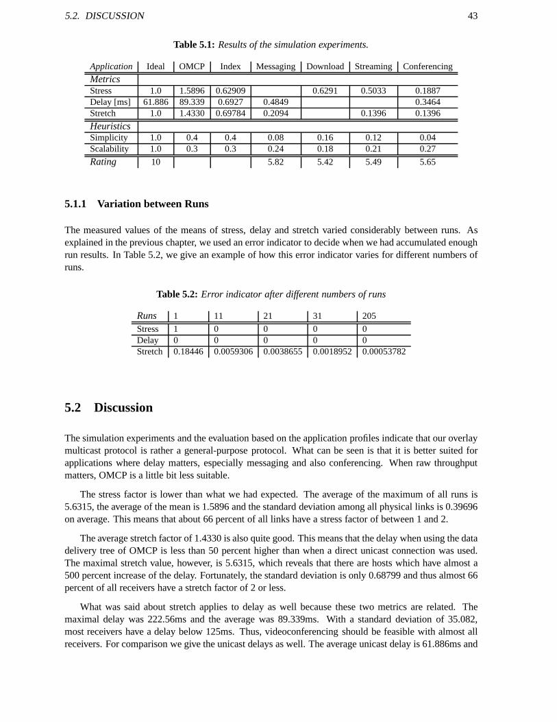
5.2. DISCUSSION 43
Table 5.1: Results of the simulation experiments.
Application Ideal OMCP Index Messaging Download Streaming Conferencing
MetricsStress 1.0 1.5896 0.62909 0.6291 0.5033 0.1887Delay [ms] 61.886 89.339 0.6927 0.4849 0.3464Stretch 1.0 1.4330 0.69784 0.2094 0.1396 0.1396
HeuristicsSimplicity 1.0 0.4 0.4 0.08 0.16 0.12 0.04Scalability 1.0 0.3 0.3 0.24 0.18 0.21 0.27
Rating 10 5.82 5.42 5.49 5.65
5.1.1 Variation between Runs
The measured values of the means of stress, delay and stretchvaried considerably between runs. Asexplained in the previous chapter, we used an error indicator to decide when we had accumulated enoughrun results. In Table 5.2, we give an example of how this errorindicator varies for different numbers ofruns.
Table 5.2: Error indicator after different numbers of runs
Runs 1 11 21 31 205
Stress 1 0 0 0 0Delay 0 0 0 0 0Stretch 0.18446 0.0059306 0.0038655 0.0018952 0.00053782
5.2 Discussion
The simulation experiments and the evaluation based on the application profiles indicate that our overlaymulticast protocol is rather a general-purpose protocol. What can be seen is that it is better suited forapplications where delay matters, especially messaging and also conferencing. When raw throughputmatters, OMCP is a little bit less suitable.
The stress factor is lower than what we had expected. The average of the maximum of all runs is5.6315, the average of the mean is 1.5896 and the standard deviation among all physical links is 0.39696on average. This means that about 66 percent of all links havea stress factor of between 1 and 2.
The average stretch factor of 1.4330 is also quite good. Thismeans that the delay when using the datadelivery tree of OMCP is less than 50 percent higher than whena direct unicast connection was used.The maximal stretch value, however, is 5.6315, which reveals that there are hosts which have almost a500 percent increase of the delay. Fortunately, the standard deviation is only 0.68799 and thus almost 66percent of all receivers have a stretch factor of 2 or less.
What was said about stretch applies to delay as well because these two metrics are related. Themaximal delay was 222.56ms and the average was 89.339ms. With a standard deviation of 35.082,most receivers have a delay below 125ms. Thus, videoconferencing should be feasible with almost allreceivers. For comparison we give the unicast delays as well. The average unicast delay is 61.886ms and

44 CHAPTER 5. RESULTS
the maximum is 89.929ms. This indicates, that video conferencing should be possible with all receiversif a better multicast scheme is used.
What bears repeating is that we did not assume node failures.Some qualitative results of scenarioswhere this kind of incident is allowed to happen will be discussed in Section 5.2.1.
In addition to the very compact results in Table 5.1, we will present a few plots of a session. The sourcehost has address 0 and we will focus on three of the more interesting subscribers, which are hosts 1, 9and 10. Data transmission starts at 100 seconds and ends at 700 seconds.
Delay Samples
In OMCP, the unicast delay among all hosts is periodically measured usingPing packets. Additionally,we measure the overlay delay from the source to the receiversby timestamping the packets at the sourcehost and evaluating this timestamp at the subscriber. Results of the latter measurements are shown inFigure 5.1 over the course of a session. We eliminated all hosts from the plot for which the delay wasconstant to make the figure more readable. Only after 275 seconds is the topology stable. An indicationthat the mesh improvement mechanism of OMCP works is that thedelay is monotonically nonincreasing.
Stretch Samples
By taking the quotient of the measured overlay delay and the measured unicast delay, stretch can becalculated easily. This quotient is shown in Figure 5.2 for the same run and the same hosts as the delaysamples. These two plots only make sense together. Obviously, the stretch of host 1 increases at around130 seconds, then goes down twice, while during the same timeperiod, the delay of this host decreasesin three steps to about one half of the initial value.
This can be explained by the fact that the stretch factor is calculated as the ratio of the overlaydelay and the unicast delay. Both these values are measured quantities and the measurements are subjectto queueing delays at six routers on average. Since all unicast delays are measured about every nineseconds, it can happen that the measured value of the unicastdelay decreases and thus, stretch increases.Host 10 experiences the same kind of stretch variability later in the session.

5.2. DISCUSSION 45
Figure 5.1: Delay samples of the three hosts. All other delays were constant during the session. It canbe seen, that it takes about 275 seconds from the time where the first node comes online until the overlaytopology becomes stable. This plot shows that no change thatincresases the delay occurs and thus theoptimization seems to work.
30
40
50
60
70
80
90
100 200 300 400 500 600 700 800
Time [s]
Delay Samples host[10]Delay Samples host[9]Delay Samples host[1]
Figure 5.2: Stretch samples of three hosts. This plot makes only sense when compared to the delay plotabove. Interestingly, stretch increases in the curves of hosts 1 and 10, even though the delay decreases atthe same time. This is caused by the fact that the unicast delay which as a direct influence on the stretchfactor is measured byPing packets and if they are delayed in the queue of a router, the measurementsvary.
1
1.2
1.4
1.6
1.8
2
2.2
100 200 300 400 500 600 700 800
Time [s]
Stretch Samples host[10]Stretch Samples host[9]Stretch Samples host[1]

46 CHAPTER 5. RESULTS
Data Delivery Tree
Every host maintains aparents listof hosts which he receives data packets from and achildren list ofhosts he sends or forwards data packets to. Figure 5.3 shows the number of children of four hosts. Host0 is the data source and therefore has the most children.
In Figure 5.4, the current tree parent for the same hosts is shown. (The source is omitted becauseit does not have a parent for obvious reasons.) It can be seen that all nodes eventually become directchildren of the source host 0. At first, host 9 switches its parent from 6 to the source. Thus, it becomesmore attractive for hosts 1 and 10. Host 10 also is at first a child of host 6, but after host 9 has become adirect child of the source, host 10 becomes a child of 9. Afterabout 275 seconds, it then determines thatit is best to be a direct child of the source and switches to 0. Host 1 first switches from its parent 3 to 6,but about one second later switches to host 9. About ten seconds later, it also notices that it is best to bea direct child of the source and switches to 0.
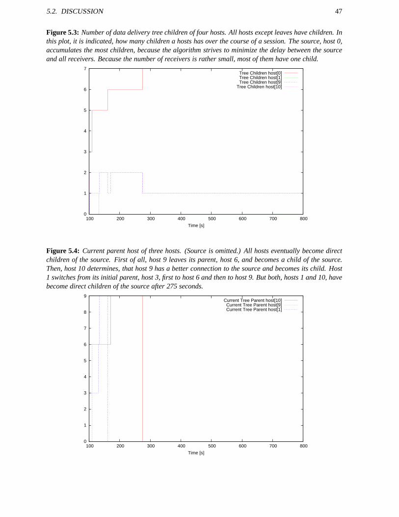
5.2. DISCUSSION 47
Figure 5.3: Number of data delivery tree children of four hosts. All hosts except leaves have children. Inthis plot, it is indicated, how many children a hosts has overthe course of a session. The source, host 0,accumulates the most children, because the algorithm strives to minimize the delay between the sourceand all receivers. Because the number of receivers is rathersmall, most of them have one child.
0
1
2
3
4
5
6
7
100 200 300 400 500 600 700 800
Time [s]
Tree Children host[0]Tree Children host[1]Tree Children host[9]
Tree Children host[10]
Figure 5.4: Current parent host of three hosts. (Source is omitted.) Allhosts eventually become directchildren of the source. First of all, host 9 leaves its parent, host 6, and becomes a child of the source.Then, host 10 determines, that host 9 has a better connectionto the source and becomes its child. Host1 switches from its initial parent, host 3, first to host 6 and then to host 9. But both, hosts 1 and 10, havebecome direct children of the source after 275 seconds.
0
1
2
3
4
5
6
7
8
9
100 200 300 400 500 600 700 800
Time [s]
Current Tree Parent host[10]Current Tree Parent host[9]Current Tree Parent host[1]

48 CHAPTER 5. RESULTS
5.2.1 Node failures
In order to provide some insight in the behaviour of OMCP in the case of node failures, we will nowpresent some plots of such a scenario. The parameters are thesame as specfified in the previous chapter,except that the paramterd_suicide_probability now has the value0.5. The source host, however,cannot die. Addionally, thet_data_interval now has the value 1, which means that the source onlyemits one packet per second.
In Figure 5.5, the status of all nodes which die during the session is shown. All nodes start in theinitial status2. When they start the joining procedure, their state is1. Once a host has joined the mesh, itsstatus becomes0. When it leaves the group, it switches its status to−1, but continues to forward packetsfor some time. If, however, a node dies abrubtly, its status becomes−2 and it stops processing packetsimmediately.
It comes as no surprise that node failures lead to packet loss. Since the source host sends one packetper second, the duration of the offline status of a host can directly be determined from the plot in Figure5.6. Host 6 misses packets twice, first when host 1 dies, and then again when host 4 stops operating. Allhosts which are not shown in this plot do not miss any data packets. The packet loss is only detectedwhen a host receives the first packet after a down time. Therefore, the death of a host and the resultingindication of packets loss do not coincide exactly.
Whenever a nodes dies which had children, they perceive packet loss. This happens first to hosts 6and 10 because their parent, host 9, dies. Later, when node 1 dies, host 6 misses packets again. Whennodes 4 and 8 die at about 440 seconds, hosts 5 and, once more, host 6 miss packets.
5.2.2 Obstacles
We were unable to perform all the simulation experiments we had planned due to the very limited time-frame of a semester project. For this reason, we only have results of one specific topology with oneparticular set of parameters. We suspect that the performance of our scheme could be improved consid-erably with the appropriate parameters. The parameters we have used in our simulation runs were mereestimations of reasonable initial values.
Missing Information There is currently no freely accessible data about the reliability of Internet back-bone routers and links. Internet service providers (ISPs) would be the natural source of such information,but it is just as natural for them to be unwilling to “admit” that their network infrastructure is not infalli-ble.
Topological Limitations Due to time constraints we could only evaluate one network topology. Thus,our results are far from representative. What’s more, the topology we used is much too small to deliverresults that can be applied to the Internet.
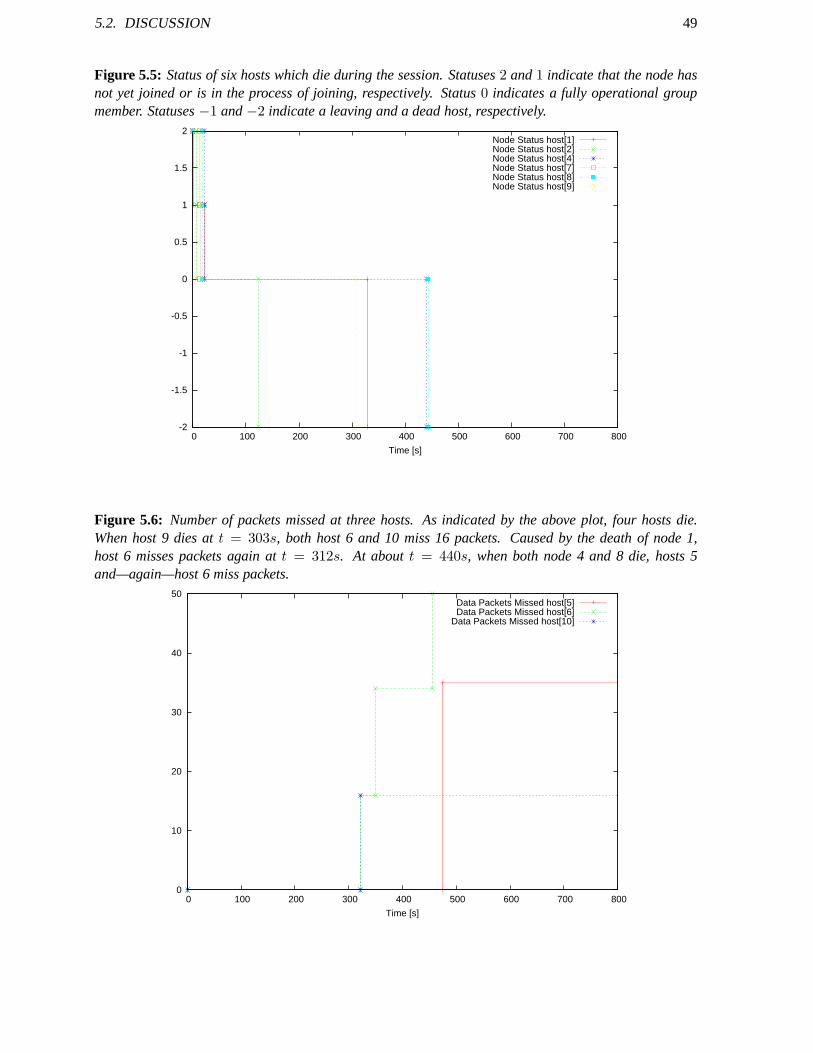
5.2. DISCUSSION 49
Figure 5.5: Status of six hosts which die during the session. Statuses2 and1 indicate that the node hasnot yet joined or is in the process of joining, respectively.Status0 indicates a fully operational groupmember. Statuses−1 and−2 indicate a leaving and a dead host, respectively.
-2
-1.5
-1
-0.5
0
0.5
1
1.5
2
0 100 200 300 400 500 600 700 800
Time [s]
Node Status host[1]Node Status host[2]Node Status host[4]Node Status host[7]Node Status host[8]Node Status host[9]
Figure 5.6: Number of packets missed at three hosts. As indicated by the above plot, four hosts die.When host 9 dies att = 303s, both host 6 and 10 miss 16 packets. Caused by the death of node1,host 6 misses packets again att = 312s. At aboutt = 440s, when both node 4 and 8 die, hosts 5and—again—host 6 miss packets.
0
10
20
30
40
50
0 100 200 300 400 500 600 700 800
Time [s]
Data Packets Missed host[5]Data Packets Missed host[6]
Data Packets Missed host[10]
Chapter 6
Conclusion
We designed an overlay multicast scheme based onNarada,and implemented it in the network simulatorOMNeT++. With this simulator, we have conducted a sufficient number of runs to be able to gatherstatistically sound values for stretch, delay and stress ofone topology and with one set of parameters.
A lot of work could not be done because our time budget was verylimited. The behaviour of ourscheme under conditions where nodes, routers or links fail,could not be analyzed. However, from a fewtest runs, it appears that our scheme isnot suitable for scenarios where node failures are likely becausepacket loss in this kind of event is too high for most multicast applications, even for fault-tolerant oneslike media streaming.
6.1 Further Research
One of the key problems of our scheme is its missing resilience against node failures. As a possiblecounter measure, we suggest multi-path routing. Additionally, it would be necessary to add a mechanismwhich allows to immediately detect when a nodes loses its parent in the data delivery tree.
Instead of flooding the network with dedicated probe packetsto measure the performance of links,ordinary control packets could be used for this purpose. This would allow a more continuous monitoringof the performance of the underlying network at no additional cost.
The current version of our scheme uses a lot of very small control packets. This could be avoidedby simply concatenating the payload of these packets into bigger “summary” packets. Furthermore, datapackets could be used to deliver control information as well.
With the extensions sketched above, our scheme might be better suited for real world scenarios. Itwould be very interesting to analyze, how resilient it is against the kinds of failures that occur in theInternet in a large-scale evaluation.
50
Appendix A
Conceptual Formulation
On pages 52 to 59, the complete conceptual formulation is given. A review of the project goals reachedand not reached follows in appendix B on page 60.
51
52 APPENDIX A. CONCEPTUAL FORMULATION

53

54 APPENDIX A. CONCEPTUAL FORMULATION

55

56 APPENDIX A. CONCEPTUAL FORMULATION

57

58 APPENDIX A. CONCEPTUAL FORMULATION
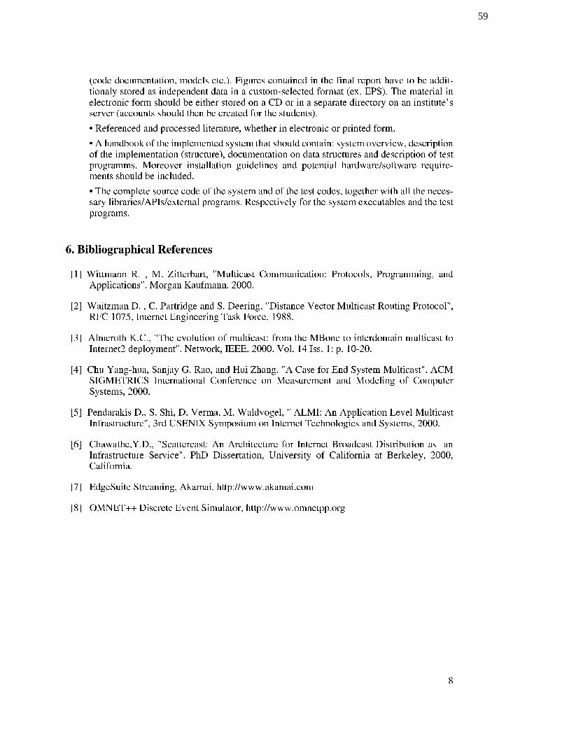
59

Appendix B
Review
From the initial plan, to implement two overlay multicast schemes and compare them to a native multicastscheme, about one third—the implementation and evaluationof one overlay multicast scheme—wasachieved. However, the performance of this custom scheme appears to be far better compared to theoriginal scheme it has been derived from.
The lessons to be learnt in this kind of semester project are:
1. Effectively find and study related work.
2. Develop sound criteria to classify related work and existing solutions and select the most represen-tative of them.
3. Design a procedure to perform a fair, reproducible and comprehensive comparison of a set of solu-tions.
4. Usage of a network simulator.
5. Implementation of a distributed algorithm, i.e. a multicast protocol running on several nodes.
6. Select parameters of interest and develop the facilitiesto measure them accurately.
7. Process huge amounts of data and derive statistically sound conclusions if possible.
Even though only one protocol could be implemented and tested, the above—and a lot more—has beenlearnt thoroughly.
One of the key learnings is the importance of implementation. Or in the words of somebody whoobviously has learnt this lesson long ago:
We reject: kings, presidents, and voting.We believe in: rough consensus and running code.
Dave Clark, IETF
60

Appendix C
OMCP Implementation
In this chapter we will first specify all simulation parameters of our overlay multicast scheme OMCP andthen present a few excerpts from the source code of the implementation in OMNeT++.
C.1 Simulation Parameters
There are a great number of parameters governing the performance of OMCP. With most of them, thereis a trade-off between efficiency and speed as well as resilience against node failures. In general, to makethe protocol faster and more adaptable to changes in the scenario, more control traffic is necessary.
The numerical values of the parameters in the following listwere determined by hand and are in noway proven to be sound by simulation experiments.
The first character of a parameter name indicates its type.
• t_... are time parameters and can be specified either in seconds or with the OMNeT++ timenotation as follows:ns for nanoseconds,us for microseconds,ms for milliseconds,s for seconds,m for minutes,h for hours andd for days.
• d_... are double parameters, mostly probabilities.
• n_... are integer parameters, mostly numbers of items.
C.1.1 Join, Leave And Death Events
• t_duration = 1000s: Duration of one simulation run.
• double_join_probability = 1.0: Probability that a node will join the group.
• t_join_time_begin = 10,
• t_join_time_end = 100: Beginning and end of the interval within which a node that has deter-mined that it will join the group sends its initial join request to the other group members. The exactjoin time is calculated randomly according to a uniform distribution.
• double_leave_probability = 0.5: Probability that a node will leave the group at some point intime.
• t_leave_time_begin = 600,
61

62 APPENDIX C. OMCP IMPLEMENTATION
• t_leave_time_end = 700: Beginning and end of the interval within which a node that has deter-mined that it will leave the group starts the leave procedure. The exact leave time is calculatedrandomly according to a uniform distribution.
• double_suicide_probability = 0.0: Probability that a node will fail abruptly at some point intime.
• t_suicide_time_begin = 100,
• t_suicide_time_end = 700: Beginning and end of the interval within which a node that hasdetermined that it will suffer of an abrubt node failure dies. The exact death time is calculatedrandomly according to a uniform distribution.
• bool_alive = true: With this parameter, a node can be defined to be dead from the beginning bysetting it equal tofalse.
C.1.2 Bootstrap Process
• n_bootstrap_nodes_known = 3: Number of other group members a node knows when bootstrap-ping the protocol. They are chosen randomly according to a uniform distribution from all validgroup member addresses. This set might contain nodes which join only after this node or which arealready dead or which will never be alive.
• n_bootstrap_nodes = 2: Number of nodes that will actually be contacted in the bootstrap pro-cess. They are chosen randomly according to a uniform distribution from the above set of candi-dates.
• t_bootstrap_timeout = 10s: Time to wait for successful connection with the group beforerestarting the bootstrap process with a new selection from the candidates set.
C.1.3 Refresh Mechanism
• t_refresh_interval = 500ms: Interval between dissemination of refresh messages.
• n_refresh_size = 100: Maximal number of nodes contained in a refresh message.
• t_refresh_timeout = 2s: Time to wait for the next refresh message of a mesh neighbor beforesending probe messages to check its status.
C.1.4 Routing Protocol
• t_routing_latency_initial = 1s: Initial latency of newly detected routes which have not beenevaluated using ping packets yet.
• t_routing_update_interval = 2s: Interval between dissemination of routing update messages.
• t_routing_update_delay = 200ms: Minimal time between triggered routing updates.
• t_routing_lifespan = 15s: Lifespan of routing information.
• t_routing_poison = 100s: Poison to add to routes which have expired or which pass notablydead nodes.
• n_routing_update_size = 50: Maximal number of route entries in a routing update packet.
• n_routing_update_path_size = 20: Maximal length of a path in a routing update packet.
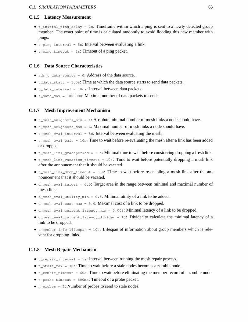
C.1. SIMULATION PARAMETERS 63
C.1.5 Latency Measurement
• t_initial_ping_delay = 2s: Timeframe within which a ping is sent to a newly detected groupmember. The exact point of time is calculated randomly to avoid flooding this new member withpings.
• t_ping_interval = 5s: Interval between evaluating a link.
• t_ping_timeout = 1s: Timeout of a ping packet.
C.1.6 Data Source Characteristics
• adr_t_data_source = 0: Address of the data source.
• t_data_start = 100s: Time at which the data source starts to send data packets.
• t_data_interval = 10ms: Interval between data packets.
• n_data_max = 1000000: Maximal number of data packets to send.
C.1.7 Mesh Improvement Mechanism
• n_mesh_neighbors_min = 4: Absolute minimal number of mesh links a node should have.
• n_mesh_neighbors_max = 6: Maximal number of mesh links a node should have.
• t_mesh_eval_interval = 5s: Interval between evaluating the mesh.
• t_mesh_eval_wait = 10s: Time to wait before re-evaluating the mesh after a link has been addedor dropped.
• t_mesh_link_graceperiod = 10s: Minimal time to wait before considering dropping a fresh link.
• t_mesh_link_vacation_timeout = 10s: Time to wait before potentially dropping a mesh linkafter the announcment that it should be vacated.
• t_mesh_link_drop_timeout = 60s: Time to wait before re-enabling a mesh link after the an-nouncement that it should be vacated.
• d_mesh_eval_target = 0.5: Target area in the range between minimal and maximal numberofmesh links.
• d_mesh_eval_utility_min = 0.5: Minimal utility of a link to be added.
• d_mesh_eval_cost_max = 5.0: Maximal cost of a link to be dropped.
• d_mesh_eval_current_latency_min = 0.002: Minimal latency of a link to be dropped.
• d_mesh_eval_current_latency_divider = 10: Divider to calculate the minimal latency of alink to be dropped.
• t_member_info_lifespan = 10s: Lifespan of information about group members which is rele-vant for dropping links.
C.1.8 Mesh Repair Mechanism
• t_repair_interval = 5s: Interval between running the mesh repair process.
• t_stale_max = 30s: Time to wait before a stale nodes becomes a zombie node.
• t_zombie_timeout = 60s: Time to wait before eliminating the member record of a zombie node.
• t_probe_timeout = 500ms: Timeout of a probe packet.
• n_probes = 2: Number of probes to send to stale nodes.

64 APPENDIX C. OMCP IMPLEMENTATION
C.1.9 Tree Transient Data Forwarding Characteristics
• t_tree_branch_transient_send = 30s: Time to continue forwarding data packets to former treechildren.
• t_tree_branch_transient_receive = 60s: Time to accept data packets from a former tree par-ent.
C.2 Excerpts from the OMCP Source Code
C.2.1 OMCP Node Class
C.2.2 Member Record Class Header File
This is the header file of the member records of OMCP nodes. Every OMCP node keeps such a memberrecord for all currently online group members. It is used to store information about the status of amember, about the overlay link to it and about its routing table. The latter is used to improve the meshas well as for the construction of the data delivery tree.
// File name: MemberRecord.h
/∗ Models record of a group member. According to the specification∗ of Narada, the record must contain the address , the last sequence∗ number seen by this address and the timestamp of the last seq.∗ number. In OMC, there are a few other things to be kept in a∗ member record.∗/
10 #ifndef MEMBERRECORD_DECL#define MEMBERRECORD_DECL
#include < vector>#include "csimul .h"#include " esmdefinitions .h"#include " routingTable .h"#include "RefreshTimeout_m.h"#include "ZombieTimeout_m.h"#include "ProbeTimeout_m.h"
20 #include "PingTimeout_m.h"#include "RoutingRequestTimeout_m.h"#include "MeshLinkVacationTimeout_m.h"#include "MeshLinkDropTimeout_m.h"
using namespacestd;
class MemberRecord{
// member fields30 private :
int memberAddress;int status ;
/∗ Mesh dynamics∗/
C.2. EXCERPTS FROM THE OMCP SOURCE CODE 65
// Status of this mesh linkint meshLinkStatus;MeshLinkVacationTimeout∗ meshLinkVacationTimeoutPtr;MeshLinkDropTimeout∗ meshLinkDropTimeoutPtr;
40 // Timestamp when adding a mesh link to this node// was last evaluatedsimtime_t meshLinkEvaluatedTimestamp;// Timestamp when the measured latency was last updatedsimtime_t latencyTimestamp;// Timestamp when this node was added to the mesh.// If zero , then there currently exists no link to itsimtime_t meshLinkAddedTimestamp;// Timestamp when this node was dropped from the mesh// If zero , then there never was a link .
50 simtime_t meshLinkDroppedTimestamp;
// Timestamp when this node was added to the tree as a child .// If zero , then there currently exists no link to itsimtime_t treeChildAddedTimestamp;// Timestamp when this node was dropped from the tree .// If zero , then there never was a link .simtime_t treeChildDroppedTimestamp;
// Timestamp when this node was added to the tree as a parent .60 // If zero , then there currently exists no link to it
simtime_t treeParentAddedTimestamp;// Timestamp when this node was dropped from the tree .// If zero , then there never was a link .simtime_t treeParentDroppedTimestamp;
double linkUtility ;int linkCost ;
/∗ Tree70 ∗/
// Timestamp when this node was added to the tree .// If zero , then there currently exists no branch to itsimtime_t treeBranchAddedTimestamp;// Timestamp when this node was dropped from the mesh// If zero , then there never was a branch.simtime_t treeBranchDroppedTimestamp;
/∗ Refresh∗/
80 // Sequence number sent in last refresh messageint lastRefreshSeqNumber;
RefreshTimeout∗ refreshTimeoutPtr ;
/∗ Routing∗/
// Pointer to track RoutingRequestTimeout messageRoutingRequestTimeout∗ routingRequestTimeoutPtr;// Member’s routing table from RoutingUpdate messages
90 // Used for construction of the data delivery treeRoutingTable routingTable ;
66 APPENDIX C. OMCP IMPLEMENTATION
// Sequence number sent in last routing update messageint lastRoutingSeqNumber;// Timestamp when routing information of this node was last updatedsimtime_t routingTimestamp;
/∗ Probing∗/
// Sequence number∗sent∗ in last probe reply to this member100 int lastSentProbeSeqNumber;
// Sequence number∗received∗ in last probe reply from this memberint lastReceivedProbeSeqNumber;// Pointer to track ProbeTimeout messageProbeTimeout∗ probeTimeoutPtr;// Counter to track how many probes have been sent to this memberint probeCount;// Timestamp when last probe to this node was sentsimtime_t probeTimestamp;
110 ZombieTimeout∗ zombieTimeoutPtr;
/∗ Pinging∗/
// Pointer to track PingTimeout messagePingTimeout∗ pingTimeoutPtr;// Sequence number∗sent∗ in last ping reply to this memberint lastSentPingSeqNumber;// Sequence number∗received∗ in last ping reply from this memberint lastReceivedPingSeqNumber;
120 // Timestamp when last ping to this node was sentsimtime_t pingTimestamp;// Latency local node to this member (from probe cycle )simtime_t latency ;
// Member’s routing table from PingReply messages// Used for evaluation of utility of adding a mesh link// and cost of dropping a mesh linkRoutingTable meshRoutingTable;
130 // Refresh cycle timestampsimtime_t refreshTimestamp;
public :
// constructorMemberRecord(int ,int ,simtime_t ,simtime_t) ;
// destructor~MemberRecord();
140// operator =void operator=(const MemberRecord &);
/∗ access methods∗/
int getAddress()const;

C.2. EXCERPTS FROM THE OMCP SOURCE CODE 67
int getStatus ()const;150 void setStatus (int ) ;
int getMeshLinkStatus()const;void setMeshLinkStatus(int ) ;
MeshLinkVacationTimeout∗ getMeshLinkVacationTimeoutPtr()const;void setMeshLinkVacationTimeoutPtr(MeshLinkVacationTimeout∗);MeshLinkDropTimeout∗ getMeshLinkDropTimeoutPtr()const;void setMeshLinkDropTimeoutPtr(MeshLinkDropTimeout∗);
160 simtime_t getMeshLinkEvaluatedTimestamp()const;void setMeshLinkEvaluatedTimestamp(simtime_t);
simtime_t getMeshLinkAddedTimestamp()const;void setMeshLinkAddedTimestamp(simtime_t);
simtime_t getMeshLinkDroppedTimestamp()const;void setMeshLinkDroppedTimestamp(simtime_t);
simtime_t getTreeChildAddedTimestamp()const;170 void setTreeChildAddedTimestamp(simtime_t);
simtime_t getTreeChildDroppedTimestamp()const;void setTreeChildDroppedTimestamp(simtime_t);
simtime_t getTreeParentAddedTimestamp()const;void setTreeParentAddedTimestamp(simtime_t);
simtime_t getTreeParentDroppedTimestamp()const;void setTreeParentDroppedTimestamp(simtime_t);
180int getRefreshSeqNum()const;void setRefreshSeqNum(int );
int getRoutingSeqNum()const;void setRoutingSeqNum(int );
int getSentPingSeqNum()const;int getNextSentPingSeqNum();void setSentPingSeqNum(int );
190int getReceivedPingSeqNum()const;int getNextReceivedPingSeqNum();void setReceivedPingSeqNum(int );
int getSentProbeSeqNum()const;int getNextSentProbeSeqNum();void setSentProbeSeqNum(int );
int getReceivedProbeSeqNum()const;200 int getNextReceivedProbeSeqNum();
void setReceivedProbeSeqNum(int );
simtime_t getRefreshTimestamp()const;

68 APPENDIX C. OMCP IMPLEMENTATION
void setRefreshTimestamp(simtime_t) ;
adr_t getNextHop()const;void setNextHop(adr_t) ;
int getNumberOfMeshRoutes()const;210 int getNumberOfMeshRoutesTo(adr_t);
RouteEntry∗ getMeshRoute(int ) const;RouteEntry∗ getMeshRouteTo(adr_t)const;adr_t getMeshNextHop(adr_t);adr_t getMeshHop(adr_t,int ) ;simtime_t getMeshLatency(adr_t) ;void addMeshRoute(adr_t, adr_t , simtime_t , simtime_t) ;void addMeshRoute(adr_t dest , adr_t next ,
simtime_t lat , simtime_t , vector<adr_t >:: iterator path ,int length ) ;
220 void addMeshRoute(RouteEntry∗);void setMeshRoute(adr_t , adr_t , simtime_t , simtime_t) ;void clearMeshRoutes() ;
int getNumberOfMemberRoutes()const;int getNumberOfMemberRoutesTo(adr_t);RouteEntry∗ getMemberRouteEntry(int ) const;RouteEntry∗ lookupMemberRouteEntry(adr_t);adr_t getMemberNextHop(adr_t);adr_t getMemberHop(adr_t,int ) ;
230 simtime_t getMemberLatency(adr_t);void addMemberRoute(adr_t, adr_t , simtime_t , simtime_t) ;void addMemberRoute(adr_t dest, adr_t next ,
simtime_t lat , simtime_t , vector<adr_t >:: iterator path ,int length ) ;
void addMemberRoute(RouteEntry∗);void setMemberRoute(adr_t, adr_t , simtime_t , simtime_t) ;void clearMemberRoutes();
ZombieTimeout∗ getZombieTimeoutPtr()const;240 void setZombieTimeoutPtr(ZombieTimeout∗);
RefreshTimeout∗ getRefreshTimeoutPtr ()const;void setRefreshTimeoutPtr (RefreshTimeout∗);
ProbeTimeout∗ getProbeTimeoutPtr()const;void setProbeTimeoutPtr(ProbeTimeout∗);
PingTimeout∗ getPingTimeoutPtr()const;void setPingTimeoutPtr (PingTimeout∗);
250RoutingRequestTimeout∗ getRoutingRequestTimeoutPtr()const;void setRoutingRequestTimeoutPtr(RoutingRequestTimeout∗);
int getProbeCount()const;void setProbeCount(int ) ;void incrementProbeCount(int ) ;void incrementProbeCount();
simtime_t getProbeTimestamp()const;

C.2. EXCERPTS FROM THE OMCP SOURCE CODE 69
260 void setProbeTimestamp(simtime_t) ;
simtime_t getPingTimestamp()const;void setPingTimestamp(simtime_t) ;
simtime_t getRoutingTimestamp()const;void setRoutingTimestamp(simtime_t) ;
simtime_t getLatencyTimestamp()const;void setLatencyTimestamp(simtime_t) ;
270simtime_t getLatency ()const;void setLatency (simtime_t) ;
double getLinkUtility () const;void setLinkUtility (double);
int getLinkCost() const;void setLinkCost(int ) ;
280 // CAUTION:// This enum has to be kept in sync with the enum memberStatus// of class ESMNode in file esmnode.henummemberStatus {freshMember,staleMember,probedMember,
zombieMember};// CAUTION:// This enum has to be kept in sync with the enum meshLinkStatus// of class ESMNode in file esmnode.henummeshLinkStatus {unusedLink, activeLink , forsakenLink};
290};
#endif
OMCP Node Routing Update Handler Method
This is one of the about 100 methods of the OMCP node class. It handles RoutingUpdate packets whichcontain the conplete routing table of another group member.OMCP uses path information in order toavoid routing loops. Additionally, routes may be poisoned to indicate that they are either scheduled to betorn down or they are already considered to be down.
// File name: OMCNode.cc
// [...]
/∗ Handles received routing update messages∗ 1. Check, if a member record for the sender exists and if a∗ mesh link to the sender is active . If not , ignore the packet .∗ 2. Check, if the sequence number in the packet is greater than∗ the routing sequence number stored in the member record. If not ,
10 ∗ ignore the packet .∗ 3. Update the routingTimestamp in the member record of the sender.∗ 4. Process route after route in the packet as follows :

70 APPENDIX C. OMCP IMPLEMENTATION
∗ 4.1. Put the whole routing table contained in the packet intoour∗ member record of the sender.∗ 4.2. Check, if the advertised path contains our address . If yes ,∗ ignore the entry .∗ 4.3. Calcualte the effective latency to the destination :∗ newLatency = ( latency advertised by sender)+(latency to sender)∗ − If the sender is −− according to the current routing
20 ∗ table −− our next hop to the destination :∗ Replace our current route with the route from the packet∗ − If the sender is not currently our next hop, but newLatency∗ is less than our current latency to the destination : Replace∗ our current route with the route from the packet∗ − Else ignore the route .∗/
void ESMNode::routingUpdateHandler(RoutingUpdate∗ ru){
30 adr_t senderAddr = ru−>getSrc();
// Get the member recordMemberRecord∗ sender = locateGroupMemberRecord(senderAddr);// Check if the pointer appears reasonableif ( sender == NULL) {
return ;}else {
int senderStatus = sender−>getStatus() ;40 int senderLinkStatus = sender−>getMeshLinkStatus();
if ( senderStatus != freshMember){return ;
}if ( senderLinkStatus == forsakenLink){
return ;}bool fromMeshNeighbour =false;if ( meshNeighbourExists(senderAddr)) {
// Sender is mesh neighbor.50 fromMeshNeighbour =true;
}else {
// Sender is not mesh neighbor and probably// wants to evaluate adding a mesh link to us
}
// Check if the sequence number is greater than the lastint seqNum =static_cast<int >(ru−>getSeqNum());if ( seqNum > sender−>getRoutingSeqNum()) {
60 // Update routing sequence numbersender−>setRoutingSeqNum(seqNum);
/∗ Process routing update∗/
// Current routing table in the member record of the sender
// Clear the routing table in the member record

C.2. EXCERPTS FROM THE OMCP SOURCE CODE 71
// We will add all routes anew as we process the70 // routing update
sender−>clearMemberRoutes();
// Get the length of the paths to be able to demux themint maxPathLength =static_cast<int >(ru−>getPathLength());
// Get the latency from local node to sender of this// RoutingUpdate.// We look in the MemberRecord for this because we measure the// latency with pings and then write the latency into the
80 // MemberRecord in method "pingReplyHandler()"simtime_t senderLatency = sender−>getLatency();if ( senderLatency < 0) {
// Something went wrong. Should never happen.senderLatency = t_routing_latency_initial_M ;
}
// Number of entries in this RoutingUpdateunsigned int numEntries = ru−>getNumEntries();
90 /∗ Check if the mesh link to the sender is active .∗ If its status is forsakenLink , then check if it uses∗ us as next hop for any route .∗ If yes , then we need to reschedule the VacationTimeout∗ because we wait until all routes have left this link .∗/
bool forsakenLinkStillUsed =false;
/∗ Check if we received one or more poisoned routes we∗ believed were good. If yes , we send out routing updates
100 ∗ in at most t_routing_update_delay_M seconds.∗/
bool sendUpdatesImmediately =false;
// Go through all vectors in RoutingUpdate// simultaneously with index ifor ( unsigned int i = 0; i < numEntries; i++){
// Get the destination address of this routeadr_t destAddr =static_cast<adr_t>(ru−>getDestination( i ) ) ;
110 /∗∗ RoutingUpdate conventions:∗ − The very first entry is always of the form∗ Destination = <senderAddress> NextHop = <senderAddress>∗ Latency = 0;∗ − The following entries have different destinations than∗ <senderAddress>.∗ − The end of valid entries is reached if an entry to∗ destination <senderAddress> appears.∗/
120if ( i > 0 && destAddr == senderAddr) {
// This route must be invalid . Quit processing this packetbreak;
}

72 APPENDIX C. OMCP IMPLEMENTATION
else {
/∗ Valid route∗/
130 // Update the routing information timestamp// of the sendersender−>setRoutingTimestamp(simTime());
adr_t nextHop =static_cast<adr_t>(ru−>getNextHop(i));simtime_t lat = static_cast<simtime_t>(ru−>getLatency(i)) ;
/∗ Copy the path into a vector and check if it contains∗ our address . If yes , ignore the entire entry and go∗ to the next .
140 ∗/bool pathContainsUs =false;// Get the beginning of the path in the arrayint base = maxPathLength∗ i ;// Set the index in the path for this record to the first hopint pathIndex = base;// Count the number of valid hops in the pathint pathLength = 0;vector<adr_t> pathVector ;pathVector . clear () ;
150 // Set the first hop in the path to// the sender of this packetpathVector .push_back(senderAddr);pathLength++;for ( int hop = 0; hop < maxPathLength; hop ++) {
pathIndex = base + hop;adr_t hopAddr = ru−>getPath(pathIndex);// Check if this is a valid hop addressif (hopAddr ==this−>localAddress_M){
// Set variable to not incorporate this route into our160 // routing table . But we still need the whole path
// to put it in the member record of the sender.pathContainsUs =true ;pathVector .push_back(hopAddr);pathLength++;
}else if(hopAddr != ROUTING_NO_HOP){
pathVector .push_back(hopAddr);pathLength++;
}170 else{
break;}
}
/∗ Update routing tables∗∗ − If this RoutingUpdate was sent by a mesh neigbhbour:∗ Add the routes to our routing table if they seem useful .∗ − Else only add them to the MemberRecord of the sender.
180 ∗/
C.2. EXCERPTS FROM THE OMCP SOURCE CODE 73
/∗ Copy routing information into the member record of the∗ sender∗ At the beginning , we cleared the routing table . Therefore ,∗ we can now just create a new entry for all routes found.∗ We won’t add routes which are poisoned , however.∗/
// Check, if this route has been poisoned , i .e ., its190 // latency is equal to or greater than t_routing_poison_M
bool poisonedRoute =false;if (! ( lat < t_routing_poison_M)){
poisonedRoute =true ;}if (! poisonedRoute){
vector<adr_t >:: iterator pathIter = pathVector .begin () ;/∗ The first entry in the path vector is the address of∗ the sender . We only need this in our own routing table .∗ Therefore , we increment the pathIter once here .
200 ∗ Example: path vector is "3 2 1".∗ − Our routing table will contain :∗ dest : 1, next : 3, path length : 3, path : 3 2 1∗ − The member routing table of sender 3 will contain only:∗ dest : 1, next : 2, path length : 2, path : 2 1∗/pathIter ++;sender−>addMemberRoute(destAddr, nextHop, lat, simTime(),
pathIter , pathLength− 1) ;}
210if ( fromMeshNeighbour){
/∗ Update our routing table∗/
// Ignore routes to usif ( destAddr ==this−>localAddress_M){
continue;}
220// Check, if we already have an entry for this destinationRouteEntry∗ re = routes_M.lookupEntry(destAddr) ;if ( re == NULL){
/∗ New destination∗/
// If the path contains us , ignore the route .if ( pathContainsUs){
230 if ( senderLinkStatus == forsakenLink){// The mesh link to the sender should be vacated , but// this member is still using us in this route .// We need to wait some more time.forsakenLinkStillUsed =true ;
}continue;

74 APPENDIX C. OMCP IMPLEMENTATION
}
// We won’t add a new route if it is poisoned.240 simtime_t effectiveLatency = lat + senderLatency;
if (! poisonedRoute){
// Create new route entry in the tablevector<adr_t>:: iterator pathIter = pathVector .begin() ;routes_M.addRoute(destAddr, senderAddr,
effectiveLatency , simTime() , pathIter , pathLength) ;}
}else {
250/∗ Known destination∗/
// Calculate the effective latency if we took this route// with the sender as next hopsimtime_t effectiveLatency = lat + senderLatency;simtime_t currentLatency = re−>getLatency();bool updateRoute =false;// Update the entry if the sender is currently our next// hop because in this case , the sender is authoritative
260 // about link failures etc .adr_t currentNextHop = re−>getNextHop();if ( senderAddr == currentNextHop){
// If the path contains us , we need to poison// this route to avoid a routing loop.if ( pathContainsUs){
routes_M.poisonRouteTo(destAddr, t_routing_poison_M);continue;
}else if ( poisonedRoute) {
270 // If the route is poisoned:// 1. Check if we already have poisoned the route in// our routing table . If not we set the latency to// our own value of a poisoned route and send// routing updates to our neighbors immediatley ,// i .e . set sendUpdatesImmediatley to trueif ( ceil ( currentLatency ) == ceil (t_routing_poison_M)){
// We already know that this route is poisoned.}else {
280 routes_M.poisonRouteTo(destAddr,t_routing_poison_M);
// Set this variable to true to make sure we send// this information to our neighbors immediately .sendUpdatesImmediately =true ;continue;
}}else {
updateRoute =true ;290 // Check if our current route in the routing table is
// poisoned.// If yes , we send routing updates to our neighbors
C.2. EXCERPTS FROM THE OMCP SOURCE CODE 75
// immediatley , i .e . set sendUpdatesImmediatley to// trueif ( ceil ( currentLatency ) == ceil (t_routing_poison_M)){
// Set this variable to true to make sure we send// this information to our neighbors immediately .sendUpdatesImmediately =true ;
}300 }
}// Poison the entry if the old entry is too oldelse if ( re−>getTimestamp() < simTime()− t_routing_lifespan_M) {
// If the path contains us , go to the next entry .if ( pathContainsUs){
routes_M.poisonRouteTo(destAddr, t_routing_poison_M);continue;
}else if ( poisonedRoute) {
310 // If the advertised route is poisoned , we set// the latency to our own value of a poisoned routeroutes_M.poisonRouteTo(destAddr, t_routing_poison_M);continue;
}else {
// This route seems to be valid and our current route// has expired .updateRoute =true ;
320// Check if our current route in the routing table is// poisoned.// If yes , we send routing updates to our neighbors// immediatley , i .e . set sendUpdatesImmediatley to// trueif ( ceil ( currentLatency ) == ceil (t_routing_poison_M)){
// Set this variable to true to make sure we send// this information to our neighbors immediately .sendUpdatesImmediately =true ;
330 }}
}// Change the entry if the new route is betterelse if ( effectiveLatency < currentLatency ) {
// If the path contains us , go to the next entry .if ( pathContainsUs){
continue;}else {
340 updateRoute =true ;// Check if our current route in the routing table is// poisoned.// If yes , we send routing updates to our neighbors// immediatley , i .e . set sendUpdatesImmediatley to// trueif ( ceil ( currentLatency ) == ceil (t_routing_poison_M)){
// Set this variable to true to make sure we send// this information to our neighbors immediately .
76 APPENDIX C. OMCP IMPLEMENTATION
sendUpdatesImmediately =true ;350 }
}}// Do the update if necessaryif ( updateRoute){
re−>setNextHop(senderAddr);re−>setLatency( effectiveLatency ) ;re−>setTimestamp(simTime());vector<adr_t>:: iterator pathIter = pathVector .begin() ;re−>setPath( pathIter , pathLength) ;
360 }}
}}if ( forsakenLinkStillUsed ){
// Reschedule VacationTimeoutMeshLinkVacationTimeout∗ vacationTimeout
= sender−>getMeshLinkVacationTimeoutPtr();if ( vacationTimeout != NULL){
// Seems to be a valid timeout pointer370 delete cancelEvent(vacationTimeout) ;
}sender−>setMeshLinkVacationTimeoutPtr(NULL);// Schedule a new timer to check if the link has been vacated// alreadyvacationTimeout
= newMeshLinkVacationTimeout("Mesh Link Vacation Timeout");
vacationTimeout−>setKind(MeshLinkVacationTimeoutEvent);vacationTimeout−>setMemberAddress(senderAddr);
380 sender−>setMeshLinkVacationTimeoutPtr(vacationTimeout);scheduleAt(simTime()+t_mesh_link_vacation_timeout_M,
vacationTimeout) ;}
}if ( sendUpdatesImmediately){
if ( routingUpdateEventMsg−>arrivalTime()> ceil (simTime() + t_routing_update_delay_M)){
// Cancel the current timercancelEvent(routingUpdateEventMsg);
390 // Schedule triggered updateroutingUpdateEventMsg
= newcMessage("TriggeredRouting Update Timer");routingUpdateEventMsg−>setKind(ROUTING_UPDATE_EVENT);scheduleAt(simTime()
+ t_routing_update_delay_M, routingUpdateEventMsg);}else {}
}400 }
}}
// [...]

C.2. EXCERPTS FROM THE OMCP SOURCE CODE 77
Bibliography
[1] Y. Chu, S. G. Rao, S. Seshan, H. Zhang, “A Case for End System Multicast.”Proceedings of theACM SIGMETRICS,June 2000.
[2] E. B. Shapiro. “Network Timetable.” IETF RFC 4 (Informational), March 1969.
[3] J. Postel. “Internet Protocol.” IETF RFC 791 (Standard), September 1981.
[4] D. Waitzman, C. Partridge, S. E. Deering. “Distance Vector Multicast Routing Protocol.” IETFRFC 1075 (Experimental), November 1988.
[5] J. Moy. “Multicast Extensions to OSPF.” IETF RFC 1584 (Proposed Standard), March 1994.
[6] A. Ballardie, P. Francis, J. Crowcroft. Core Based Trees. Proceedings of the ACM SIGCOMM,September 1993.
[7] A. Ballardie. “Core Based Trees (CBT) Multicast RoutingArchitecture.” IETF RFC 2201(Experimental), September 1997.
[8] A. Ballardie, B. Cain, Z. Zhang. “Core Based Trees (CBT) Multicast Routing Architecture.” IETFInternet-draft “draft-ietf-idmr-cbt-spec-v3-01.txt”,August 1998.
[9] D. Estrin, D. Farinacci, A. Helmy, D. Thaler, S. E. Deering, M. Handley, V. Jacobson, C. Liu,P. Sharma, L. Wei. “Protocol Independent Multicast – SparseMode (PIM-SM): ProtocolSpecification.” IETF RFC 2362 (Experimental), June 1998.
[10] B Fenner, M. Handley, H. Holbrook, I. Kouvelas. “Protocol Independent Multicast – Sparse Mode(PIM-SM): Protocol Specification (Revised).” IETF Internet-draft, February 2004.
[11] S. E. Deering, R. Hinden. “Internet Protocol, Version 6(IPv6) Specification.” IETF RFC 2460(Draft Standard), December 1998.
[12] J. Frankel, T. Pepper. “Gnutella.”http://rfc-gnutella.sourceforge.net/
[13] B. Cohen. “BitTorrent.”http://www.bitconjurer.org/BitTorrent/
[14] “Internet Engineering Task Force (IETF).”http://www.ietf.org/
[15] András Varga. “OMNeT++– Objective Modular Network Testbed in C++.” Discrete eventsimulation system.http://www.omnetpp.org/
[16] Georgia Institute of Technology/College of Computing. “GT-ITM –Georgia Institute ofTechnology Internet Topology Model.” Network topology generator.http://www.cc.gatech.edu/projects/gtitm/
[17] A. Tanenbaum.Computer Networks.Published by Prentice Hall PTR, 4th edidtion (August 2002),ISBN: 0130661023.
78

BIBLIOGRAPHY 79
[18] L. Peterson, B Davie.Computer Networks: A Systems Approach.Published by Morgan Kaufmann,3rd edition (May 2003), ISBN: 155860832X.
[19] J. Postel. “Transmission Control Protocol.” RFC 793 (Standard), September 1981.
[20] L. Kleinrock. “Information Flow in Large Communication Nets.” Ph.D. thesis, MassachusetsInstitute of Technology, May 1961.
[21] J. D. Day, H. Zimmermann. “The OSI Reference Model.”Proceedings of the IEEE,December1983.
[22] International Organization for Standardization. “Open System Interconnection Reference Model.”ISO/IEC Standard 7498, 1984.
[23] S. E. Deering. “Host Extensions for IP Multicasting.” IETF RFC 1112 (Standard), August 1989.
[24] S. E. Deering, D. R. Cheriton. “Host groups: A multicastextension to the Internet Protocol.”Proceedings of the ACM/IEEE Data Communications Symposium, September 1985.
[25] S. E. Deering. “Multicast Routing in Internetworks andExtended LANs.”Proceedings of the ACMSIGCOMM,August 1988.
[26] S. E. Deering. “Multicast Routing in a Datagram Internetwork.” Ph.D. thesis, Stanford University,Electrical Engineering Department, December 1991.
[27] H. Erikson. “MBONE: The Multicast Backbone.”Communications of the ACM,August 1994.
[28] T. M. Munzner, E. Hoffmann, K. Claffy, B. Fenner. “Visualizing the Global Topology of theMBone.” Proceedings of the IEEE InfoVis,October 1996.
[29] Y. Sh. Shi. “Design of Overlay Networks for Internet Multicast.” Ph.D. thesis, WashingtonUniversity, Sever Institute of Technology, August 2002.
[30] F. Lau, H. Rubin, M. H. Smith, L. Trajovic. “DistributedDenial of Service Attacks.”Proceedingsof the IEEE International Conference on Systems, Man, and Cybernetics,October 2000.
[31] H. Holbrook, D. Cheriton. “IP Multicast Channels: EXPRESS Support for Large-scale SingleSource Applications.”Proceedings of the ACM SIGCOMM,September 1999.
[32] H. Holbrook, B. Cain. “Source Specific Multicast.” IETFInternet-draft, March 2000.
[33] J. H. Saltzer, D. P. Reed, D. D. Clark. “End-To-End Arguments in System Design.”ACMTransactions on Computer Systems,November 1984.
[34] S. Banerjee, B. Bhattacharjee. “A Comparative Study ofApplication Layer Multicast Protocols.”University of Maryland, October 2002.
[35] P. Francis. “Yoid: Extending the Multicast Internet Architecture.” White paper, April 2000.http://www.aciri.org/yoid/
[36] B. Zhang, S. Jamin, L. Zhang. “Host Multicast: A Framework for Delivering Multicast to EndUsers.”Proceedings of the IEEE INFOCOM,June 2002.
[37] S. Banerjee, B. Bhattacharjee, C. Kommareddy. “Scalable Application Layer Multicast.”Proceedings of the ACM SIGCOMM,August 2002.
[38] S. RAtnasamy, P. Francis, M. Handley, R. Karp, S. Shenker. “A Scalable Content-addressableNetwork.” Proceedings of the ACM SIGCOMM,August 2001.
[39] M. Castro, P. Druschel, A-M. Kermarrec, A. Rostron. “SCRIBE: A Large-scale and DecentralizedApplication-level Multicast Infrastructure.IEEE Journal on Selected Areas in Communications(JSAC),2002.
[40] C. L. Hedrick. “Routing Information Protocol.” IETF RFC 1058, June 1988.
[41] G. Malkin. “RIP Version 2.” IETF RFC 2453 (Standard), November 1998.
80 BIBLIOGRAPHY
[42] A. S. Thyagarajan, S. E. Deering. “Hierarchical Distance-Vector Multicast Routing for theMBone.” Proceedings of the ACM SIGCOMM,August 1995.
[43] J. Moy. “OSPF specification.” IETF RFC 1131 (Proposed Standard), October 1989.
[44] J. Moy. “OSPF Version 2.” IETF RFC 2328 (Standard), April 1998.
[45] D. Pendarakis, S. Shi, D. Verma, M. Waldvogel. “ALMI: AnApplication Level MulticastArchitecture.”Proceedings of the USENIX USITS,March 2001.
[46] S. Banerjee, Ch. Kommareddy, K. Kar, B. Bhattacharjee,S. Khuller “Construction of an EfficientOverlay Multicast Infrastructure for Real-time Applications.” Proceedings of the IEEEINFOCOM,April 2003.
[47] J. Jannotti, D. K. Gifford, K. L. Johnson, M. F. Kaashoek, J. W. O’Toole, Jr. “Overcast: ReliableMulticasting with an Overlay Network.”Proceedings of the USENIX OSDI 4,October 2000.
[48] Y. D. Chawathe. “Scattercast: An Architecture for Internet Broadcast Distribution as anInfrastructure Service.” Ph.D. thesis, University of California at Berkeley, December 2000.
[49] B. Cain, S. E. Deering, I. Kouvelas, B. Fenner, A. Thyagarajan. “Internet Group ManagementProtocol, Version 3.” IETF RFC 3376 (Proposed Standard), October 2002.
[50] NIST/SEMATECH. “e-Handbook of Statistical Methods.”, July 2004.http://www.itl.nist.gov/div898/handbook/
[51] I. Busse, B. Deffner, H. Schulzrinne. “Dynamic QoS Control of Multimedia Applications based onRTP.” Proceedings of the First International Workshop on High Speed Networks and OpenDistributed Platforms,June 1995.
[52] F. Dressler: “A Metric for Numerical Evaluation of the QoS of an Internet Connection.”Proceedings of 18th International Teletraffic Congress (ITC18),August 2003.
[53] P. Clément, B. Jenkins. “Adapting Test and MeasurementTools to Centralcasting and BroadbandIP Contribution.” Thales Broadcast and Multimedia, 2003.http://www.broadcastpapers.com/testmeasurement/ThalesAdaptTestMeasTools.pdf
[54] F. Dressler. “How to Measure Reliability and Quality ofIP Multicast Services?”Proceedings of2001 IEEE Pacific Rim Conference on Communications, Computers and Signal Processing(PACRIM ’01),August 2001.
[55] Akamai. “EdgeSuite: A Comprehensive Content DeliverySolution for Advanced E-Business.”http://www.akamai.com/en/html/services/edgesuite.html
[56] University of Southern California/Information Sciences Institute. “The Network Simulator –NS-2.” Discrete event simulation system.http://www.isi.edu/nsnam/ns/
[57] K. Calvert, M. Doar, E. W. Zegura. “Modeling Internet Topology.” IEEE CommunicationsMagazine,June 1997.

Index
application layer, 7application layer multicast, 15AS, 15autonomous system, 15
CBT, 1, 20channel, 7circuit-switched, 6computer
network, 3cost, 8
data link layer, 7datagram, 10dense mode, 14DVMRP, 1, 19
end system, 3Express, 14
forwarding, 8forwarding table, 8
header, 7hop, 8host, 3host address, 10host part, 10host-based overlay multicast , 16HTTP, 11hub, 4
IGMPjoin, 21leave, 21
implicit overlay multicast , 17IP, 10IPv4, 10
multicastCBT, 1, 20DVMRP, 1, 19MOSPF, 1, 19PIM, 1, 20
IPv6, 10
join, 21
LAN, 14layer, 6
application layer, 7data link layer, 7network layer, 7physical layer, 7transport layer, 7
leave, 21level, 6local-area network, 14
mesh-first overlay multicast , 16MOSPF, 1, 19multicast, 1
dense mode, 14overlay
host-based, 16implicit, 17mesh-first, 16replicator-based, 16tree-first, 16
receiver, 13sparse mode, 14subscriber, 13
netmask, 10network, 3
circuit-switched, 6packet-switched, 6protocol, 3
network address, 10network layer, 7next hop, 8
OMCP, 20Open Shortest Path First, 19OSPF, 19overlay multicast, 15
host-based, 16implicit, 17mesh-first, 16
81
82 INDEX
replicator-based, 16tree-first, 16
packet-switched, 6physical layer, 7PIM, 1, 14, 20PIM-SM, 14port, 10protocol, 3
Express, 14header, 7HTTP, 11IP, 10IPv4, 10IPv6, 10layer, 6level, 6OMCP, 20OSPF, 19PIM, 14PIM-SM, 14RIP, 19SMTP, 11SSM, 14stack, 6TCP/IP, 10
receiver, 13rendez-vous point, 21replicator-based overlay multicast , 16reverse-path forwarding, 19RIP, 19route, 8routing, 8
protocolOSPF, 19RIP, 19
shortest path routing, 8Routing Information Protocol, 19routing table, 8RPF, 19
shared tree, 21shortest path routing, 8SMTP, 11source-specific tree, 21sparse mode, 14SSM, 14subnet, 4subnetwork, 4subscriber, 13
switching, 6
TCPport, 10
TCP/IP, 10transport layer, 7tree
shared tree, 21source-specific tree, 21
tree-first overlay multicast , 16