towards test focus selection for integration …
TRANSCRIPT

TOWARDS TEST FOCUS SELECTION FOR INTEGRATION TESTING
USING SOFTWARE METRICS
A Dissertation
Submitted to the Graduate Faculty
of the
North Dakota State University
of Agriculture and Applied Science
By
Shadi Elaiyan Bani Ta’an
In Partial Fulfillment of the Requirements
for the Degree of
DOCTOR OF PHILOSOPHY
Major Department:
Computer Science
April 2013
Fargo, North Dakota

North Dakota State University Graduate School
Title
TOWARDS TEST FOCUS SELECTION FOR INTEGRATION
TESTING USING SOFTWARE METRICS
By
Shadi Elaiyan Bani Ta’an
The Supervisory Committee certifies that this disquisition complies
with North Dakota State University’s regulations and meets the
accepted standards for the degree of
DOCTOR OF PHILOSOPHY
SUPERVISORY COMMITTEE:
Dr. Kenneth Magel
Chair
Dr. Kendal Nygard
Dr. Jim Coykendall
Dr. Jun Kong
Dr. Gursimran Walia
Approved:
4/4/2013
Dr. Brian Slator
Date
Department Chair

ABSTRACT
Object-oriented software systems contain a large number of modules which make the
unit testing, integration testing, and system testing very difficult and challenging. While the
aim of the unit testing is to show that individual modules are working properly and the aim
of the system testing is to determine whether the whole system meets its specifications, the
aim of integration testing is to uncover errors in the interactions between system modules.
Correct functioning of object-oriented software depends upon the successful integration
of classes. While individual classes may function correctly, several faults can arise when
these classes are integrated together. However, it is generally impossible to test all the
connections between modules because of time and cost constraints. Thus, it is important to
focus the testing on the connections presumed to be more error-prone.
The general goal of this research is to let testers know where in a software system to
focus when they perform integration testing to save time and resources. In this work, we
propose a new approach to predict and rank error-prone connections in object-oriented
systems. We define method level metrics that can be used for test focus selection in
integration testing. In addition, we build a tool which calculates the metrics automatically.
We performed experiments on several Java applications taken from different domains. Both
error seeding technique and mutation testing were used for evaluation. The experimental
results showed that our approach is very effective for selecting the test focus in integration
testing.
iii

ACKNOWLEDGMENTS
I sincerely thank Allah, my God, the Most Gracious, the Most Merciful for enlightening
my mind, making me understand, giving me confidence to pursue my doctoral studies at
North Dakota State University, and surrounding me by wonderful friends and family. I
would like to take this opportunity to thank them.
I would like to express my sincere thanks, gratitude and deep appreciation for Dr.
Kenneth Magel, my major advisor, for his excellent guidance, caring, assistance in every
step I went through and providing me with an excellent atmosphere for doing research.
He is a real mentor, always available, and very inspirational. Throughout my studies, he
provided encouragement, sound advice, good teaching, and lots of good ideas. I would
like to thank Dr. Kendall Nygard, my co-advisor, for his continuous support and insightful
suggestions.
I would like to thank the members of my dissertation committee, Dr. James Coykendall,
Dr. Jun Kong, and Dr. Gurisimran Walia for generously offering their precious time,
valuable suggestions, and good will throughout my doctoral tenure.
I cannot forget to mention my wonderful colleagues and friends; they not only gave
me a lot of support but also made my long journey much more pleasant. Thanks to Ibrahim
Aljarah, Qasem Obeidat, Mohammad Okour, Raed Seetan, and Talal Almeelbi. Special
thanks to my wonderful friend, Mamdouh Alenezi, for providing encouragement, caring
and great company.
My special and deepest appreciations go out to my family members to whom I owe
so much. I thank my beloved parents for their love, prayers, and unconditional support not
iv

only throughout my doctoral program but also throughout my entire life. You are wonderful
parents and I could never, ever have finished this dissertation without you.
Shadi Bani Ta’an
December 2012
v

TABLE OF CONTENTS
ABSTRACT . . . . . . . . . . . . . . . . . . . . . . . . . . . . . . . . . . . . . . . . . . . . . . . . . . . . . . . . . . iii
ACKNOWLEDGMENTS . . . . . . . . . . . . . . . . . . . . . . . . . . . . . . . . . . . . . . . . . . . . . . . iv
LIST OF TABLES . . . . . . . . . . . . . . . . . . . . . . . . . . . . . . . . . . . . . . . . . . . . . . . . . . . . . vii
LIST OF FIGURES . . . . . . . . . . . . . . . . . . . . . . . . . . . . . . . . . . . . . . . . . . . . . . . . . . . . viii
CHAPTER 1. INTRODUCTION . . . . . . . . . . . . . . . . . . . . . . . . . . . . . . . . . . . . . . . . . 1
CHAPTER 2. LITERATURE REVIEW . . . . . . . . . . . . . . . . . . . . . . . . . . . . . . . . . . . 8
CHAPTER 3. THE PROPOSED APPROACH . . . . . . . . . . . . . . . . . . . . . . . . . . . . . . 30
CHAPTER 4. EXPERIMENTAL EVALUATION . . . . . . . . . . . . . . . . . . . . . . . . . . . 48
CHAPTER 5. CONCLUSION AND FUTURE WORK . . . . . . . . . . . . . . . . . . . . . . 76
REFERENCES . . . . . . . . . . . . . . . . . . . . . . . . . . . . . . . . . . . . . . . . . . . . . . . . . . . . . . . . 80
APPENDIX. SMIT SOURCE CODE . . . . . . . . . . . . . . . . . . . . . . . . . . . . . . . . . . . . . . 86
vi
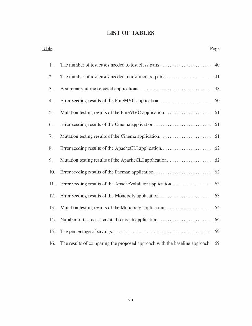
LIST OF TABLES
Table Page
1. The number of test cases needed to test class pairs. . . . . . . . . . . . . . . . . . . . . . 40
2. The number of test cases needed to test method pairs. . . . . . . . . . . . . . . . . . . . 41
3. A summary of the selected applications. . . . . . . . . . . . . . . . . . . . . . . . . . . . . . . 48
4. Error seeding results of the PureMVC application. . . . . . . . . . . . . . . . . . . . . . . 60
5. Mutation testing results of the PureMVC application. . . . . . . . . . . . . . . . . . . . 61
6. Error seeding results of the Cinema application. . . . . . . . . . . . . . . . . . . . . . . . . 61
7. Mutation testing results of the Cinema application. . . . . . . . . . . . . . . . . . . . . . 61
8. Error seeding results of the ApacheCLI application. . . . . . . . . . . . . . . . . . . . . . 62
9. Mutation testing results of the ApacheCLI application. . . . . . . . . . . . . . . . . . . 62
10. Error seeding results of the Pacman application. . . . . . . . . . . . . . . . . . . . . . . . . 63
11. Error seeding results of the ApacheValidator application. . . . . . . . . . . . . . . . . 63
12. Error seeding results of the Monopoly application. . . . . . . . . . . . . . . . . . . . . . . 63
13. Mutation testing results of the Monopoly application. . . . . . . . . . . . . . . . . . . . 64
14. Number of test cases created for each application. . . . . . . . . . . . . . . . . . . . . . . 66
15. The percentage of savings. . . . . . . . . . . . . . . . . . . . . . . . . . . . . . . . . . . . . . . . . . . 69
16. The results of comparing the proposed approach with the baseline approach. 69
vii

LIST OF FIGURES
Figure Page
1. The dependency relationship between component A and component B. . . . . 8
2. The ”V” model of software testing. . . . . . . . . . . . . . . . . . . . . . . . . . . . . . . . . . . . 11
3. An example of coverage criteria. . . . . . . . . . . . . . . . . . . . . . . . . . . . . . . . . . . . . . 13
4. An example of top-down strategy. . . . . . . . . . . . . . . . . . . . . . . . . . . . . . . . . . . . . 19
5. An example of bottom-up strategy. . . . . . . . . . . . . . . . . . . . . . . . . . . . . . . . . . . . 20
6. An example of big-bang strategy. . . . . . . . . . . . . . . . . . . . . . . . . . . . . . . . . . . . . 20
7. An overview of the proposed approach. . . . . . . . . . . . . . . . . . . . . . . . . . . . . . . . 30
8. Toy system. . . . . . . . . . . . . . . . . . . . . . . . . . . . . . . . . . . . . . . . . . . . . . . . . . . . . . . 32
9. Dependencies of the toy system. . . . . . . . . . . . . . . . . . . . . . . . . . . . . . . . . . . . . . 33
10. Simple Java example that contains two classes MO and RO. . . . . . . . . . . . . . . 42
11. The coupling dependency graph for the Java example. . . . . . . . . . . . . . . . . . . . 43
12. An example of complex input parameter. . . . . . . . . . . . . . . . . . . . . . . . . . . . . . . 43
13. An example of maximum nesting depth. . . . . . . . . . . . . . . . . . . . . . . . . . . . . . . 43
14. An example of computing the ICM metric (ICMm1m2 = 2). . . . . . . . . . . . 44
15. An example of computing the OCM metric (OCMm1m2 = 1). . . . . . . . . . . 44
16. Our testing approach. . . . . . . . . . . . . . . . . . . . . . . . . . . . . . . . . . . . . . . . . . . . . . . 44
17. High level description of SMIT tool. . . . . . . . . . . . . . . . . . . . . . . . . . . . . . . . . . 45
18. The dependencies for completeTrade method in the Monopoly application. . 46
19. Run SMIT from command line. . . . . . . . . . . . . . . . . . . . . . . . . . . . . . . . . . . . . . . 46
viii

20. A screen capture for SMIT output. . . . . . . . . . . . . . . . . . . . . . . . . . . . . . . . . . . . 46
21. A screen capture for part of the final Report output for PureMVC. . . . . . . . . . 47
22. A toy example of classes and the dependencies between methods. . . . . . . . . . 47
23. Class-pairs for the toy system and their weights. . . . . . . . . . . . . . . . . . . . . . . . . 47
24. The class diagram of Monopoly. . . . . . . . . . . . . . . . . . . . . . . . . . . . . . . . . . . . . . 50
25. The class diagram of PureMVC. . . . . . . . . . . . . . . . . . . . . . . . . . . . . . . . . . . . . . 51
26. The class diagram of Cinema. . . . . . . . . . . . . . . . . . . . . . . . . . . . . . . . . . . . . . . . 52
27. The class diagram of the ApacheCLI. . . . . . . . . . . . . . . . . . . . . . . . . . . . . . . . . . 53
28. The class diagram of Pacman. . . . . . . . . . . . . . . . . . . . . . . . . . . . . . . . . . . . . . . . 54
29. Part of the class diagram of ApacheValidator. . . . . . . . . . . . . . . . . . . . . . . . . . . 55
30. The class diagram of JTopas. . . . . . . . . . . . . . . . . . . . . . . . . . . . . . . . . . . . . . . . . 56
31. Mutation Operators for Inter-Class Testing. . . . . . . . . . . . . . . . . . . . . . . . . . . . . 60
32. Error detection rate for the selected applications. . . . . . . . . . . . . . . . . . . . . . . . 65
ix

CHAPTER 1. INTRODUCTION
1.1. Background
Software is a fundamental component in many of the devices and the systems that are
available in modern life. It is used to control many critical functions of different machines
such as spaceships, aircrafts, and pacemakers. All of these machines are running software
systems that overly optimistic users assume will never fail. Software failure can cause
serious problems such as loss of human life. In addition, software failure can have a
major impact on economics. For example, software errors cost the United States economy
around 60 billion dollars annually according to a study conducted by the National Institute
of Standards and Technology [64]. Therefore, creating a reliable software system and
increasing the confidence of the correctness of a software system are very important. Even
though there are many methods that can be used to provide assurance that the software
is of high quality and reliability, software testing is the primary method which is used to
evaluate software under development.
Software testing is the process of executing a program or system with the intent of
finding errors [49]. Software testing is very costly. It requires approximately 50% of
software development cost [49]. Much software contains large number of errors. One
reason these errors persist through the software development life cycle is the restriction of
testing resources. These resources are restricted by many factors such as time (e.g., the
software should be delivered in specific time) and cost (e.g., testing the whole software
system requires a large team). Thus, if testing effort can be focused on the parts of a
software system where errors are most likely to occur, then the available resources can be
used more effectively, and the produced software system will be more reliable at lower
cost.
Object-oriented software is a burgeoning form of software. Object-oriented software
systems contain large number of modules which make the unit testing, integration testing,
1

and system testing very difficult and challenging. While the aim of the unit testing is
to show that the individual modules are correct and the aim of the system testing is to
determine whether the whole system meets its specifications, the aim of integration testing
is to test that the interactions between system modules are correct. Correct functioning
of object-oriented software depends upon the successful integration of classes. While
individual classes may function correctly, several new faults can arise when these classes
are integrated together. However, it is usually impossible to test all the connections between
classes. Therefore, it is important to focus the testing on the connections presumed to be
more error-prone.
Errors that happen when integrating two components can be very costly. An example
of one public failure that happened because of disagreement of assumptions was the Mars
Climate Orbiter. In September 1999, the communication with the spacecraft was lost as
the spacecraft went into orbital insertion due to a misunderstanding in the units of measure
used by two modules created by different software groups. One module computed data in
English units of pound-seconds and forwarded the data to a module that expected data in
metric units of Newtonseconds. The Mars Climate Orbiter went out of radio contact when
the spacecraft passed behind Mars 49 seconds earlier than expected, and communication
was never reestablished. This is a very typical integration error, but the error costs millions
of dollars [62].
The goal of this research is to reduce the cost and the time required for integration
testing by ranking the connections between modules and then the test cases are targeted
to test the highly ranked connections. We are aiming to provide testers with an accurate
assessment of which connections are most likely to contain errors, so they can regulate the
testing efforts to target these connections. Our assumption is that using a small number
of test cases to test the highly ranked error-prone connections will detect the maximum
number of integration errors. This work presents an approach to select the test focus in
2

integration testing. It uses method-level software metrics to specify and rank the error-
prone connections between modules of systems under test.
1.2. Motivation
Integration testing is a very important process in software testing. Software testing
cannot be effective without performing integration testing. Around 40% of software errors
are discovered during integration testing [67]. The complexity of integration testing in-
creases as the number of interactions increases. A full integration testing of a large system
may take long time to complete. Integration testing of large software systems consumes
time and resources. Applying the same testing effort to all connections of a system is not
a good approach. An effective approach to reduce time and cost of integration testing is to
focus the testing effort on parts of the program that are more likely to contain errors.
The goal of test focus selection is to select the parts of the system that have to be
tested more widely. The test focus selection is important because of time and budget
constraints. The assumption is that the integration testing process should focus on the
parts of the system that are more error-prone. Several approaches to predict error-prone
components have been proposed by researchers [7, 14, 24]. Though, these approaches
focus only on individual modules. For that reason, they can be used for unit testing but
they cannot be used for integration testing because integration testing tests the connections
between modules. Thus, predicting error-prone connections is necessary for test focus
selection in integration testing. As a result, new approaches for test focus selection in
integration testing are needed. In this work, we present a new approach to predict and rank
error-prone connections in object-oriented systems. We give a weight for each connection
using method level metrics. Then we predict the number of test cases needed to test each
connection. The general goal of this research is to tell testers where in a software system
to focus when they perform integration testing to save time and resources.
3

1.3. Terminology
This section presents a number of terms that are important in software testing and
that will be used in this work. We use definitions of software error, software fault, soft-
ware failure, test case, metric, integration testing, and object-oriented language from IEEE
standard 610.12-1990 [57].
• Software fault: An incorrect step, process, or data definition in a computer program
that can happen at any stage during the software development life cycle. Usually, the
terms ”error” and ”bug” are used to express this meaning. Faults in software system
may cause the system to fail in performing as required.
• Software error: The difference between a computed, observed, or measured value or
condition and the correct value.
• Software failure: The inability of a system or component to perform its required
functions within specified performance requirements.
• Test case: A set of test inputs, execution conditions, and expected results developed
for a particular objective, such as to exercise a particular program path or to verify
compliance with a specific requirement.
• Metric: A quantitative measure of the degree to which a system, component, or
process possesses a given attribute.
• Object-oriented language: A programming language that allows the user to express
a program in terms of objects and messages between those objects such as C++ and
Java.
• Integration testing: Testing in which software components, hardware components, or
both are combined and tested to evaluate the interaction between them.
4

1.4. Problem Statement and Objectives
This dissertation addresses one main problem: How to reduce cost and time required
for integration testing while keeping its effectiveness in revealing errors. We want to test
our hypothesis that the degree of dependency between methods is a good indicator of
the number of integration errors in the interaction between methods. We assume that a
developer usually makes more mistakes if two methods have strong dependencies. We
also assume that developer makes more mistakes if methods are complex. Therefore,
we give a weight for each connection based on both the degree of dependency and the
internal complexity of the methods. In our work, we define method level dependency
metrics to measure the degree of dependency between methods. We are just interested in
computing dependencies between methods that belong to different classes. Dependencies
between methods in the same class may be needed in unit testing but they are not needed
in integration testing.
The objective of this work is to develop a new approach for integration testing that
reduces cost and time of integration testing through reducing the number of test cases
needed while still detecting at least 80% of integration errors. The number of test cases
can be reduced by focusing the testing on the error-prone connections. We want to write
test cases that cover small number of connections while these test cases uncover most of
the integration errors. Integration testing can never recompense for inadequate unit testing.
In our approach, we assume that all of the classes have gone through adequate unit testing.
1.5. Contributions
This dissertation makes the following contributions:
1. Define method-level object-oriented metrics. We define metrics that can be used
for test focus selection in integration testing. Our metrics are defined and selected
according to the following two assumptions: 1) the degree of dependencies between
the two methods that have an interaction are strongly correlated with the number of
5

integration errors between the methods; 2) the internal complexity of the two method
that have an interaction are strongly correlated with the number of integration errors
in the interaction between them. We define four method level dependency metrics
and three method level internal complexity metrics. We also define metrics on both
method-pair and class-pair levels.
2. Build a tool to calculate the metrics automatically. We develop a tool using the R
language to compute the metrics automatically from both the source code and the
byte code. The tool produces four files in CSV format: 1) method level metrics file,
which shows the metrics values for each method in the system under test; 2) method-
pair level metrics file, which shows the metrics values for each method-pair such that
(m1 and m2) is a method-pair if method m1 calls method m2 or vice verse; 3) class-
pair level file, which shows the metrics values for each class-pair such that (c1 and
c2) is a class-pair if any method in class c1 calls any method in class c2 or vice verse.
3. Propose an approach to reduce cost and time of integration testing. We use a combi-
nation of object-oriented metrics to give a weight for each method-pair connection.
Then, we predict the number of test cases needed to test each connection. The
objective is to reduce the number of test cases needed to a large degree while still
detecting at least 80% of integration errors.
4. Conduct an experimental study on several Java applications taken from different
domains. In order to evaluate the proposed approach, we use both error seeding
and mutation analysis techniques.
1.6. Dissertation Outline
The rest of the dissertation is organized as follows: Chapter 2 starts by introducing
some areas that are related to the dissertation and then it discusses related work. Chapter
3 describes the proposed approach. The chapter starts by defining a representation for a
6

software system. Then, it explains the steps of the proposed approach. After that, a section
presents the tool that we developed for implementing the proposed approach. The chapter
ends with a toy example to explain the proposed approach. The experimental evaluation
and discussion are presented in Chapter 4. Chapter 5 concludes the dissertation and talks
about future directions.
7
CHAPTER 2. LITERATURE REVIEW
2.1. Background
This research is related to software dependencies, coupling, software testing, and
integration testing. This section introduces background material of these areas.
2.1.1. Software Dependencies
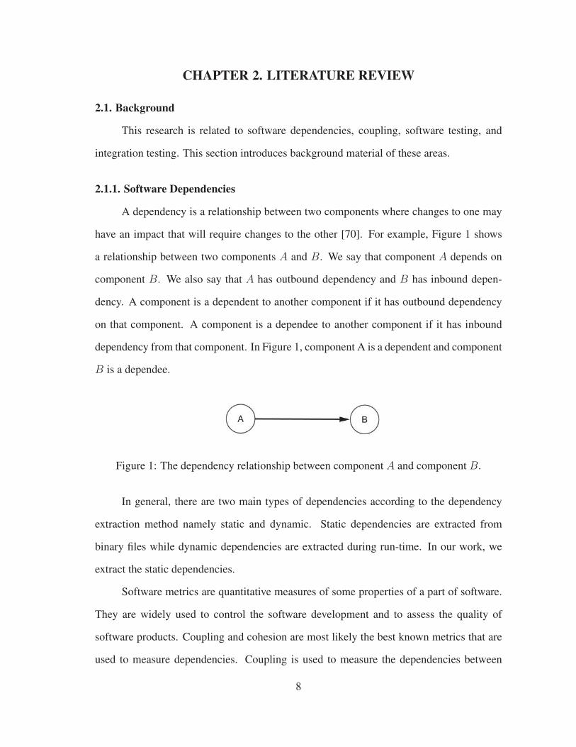
A dependency is a relationship between two components where changes to one may
have an impact that will require changes to the other [70]. For example, Figure 1 shows
a relationship between two components A and B. We say that component A depends on
component B. We also say that A has outbound dependency and B has inbound depen-
dency. A component is a dependent to another component if it has outbound dependency
on that component. A component is a dependee to another component if it has inbound
dependency from that component. In Figure 1, component A is a dependent and component
B is a dependee.
Figure 1: The dependency relationship between component A and component B.
In general, there are two main types of dependencies according to the dependency
extraction method namely static and dynamic. Static dependencies are extracted from
binary files while dynamic dependencies are extracted during run-time. In our work, we
extract the static dependencies.
Software metrics are quantitative measures of some properties of a part of software.
They are widely used to control the software development and to assess the quality of
software products. Coupling and cohesion are most likely the best known metrics that are
used to measure dependencies. Coupling is used to measure the dependencies between
8

different modules, while cohesion is used to measure the dependencies inside a single
module. Modules are considered highly coupled when there are many connections between
them. A connection is a reference from one module to another. Low coupling and high
cohesion are required to produce a good software system. In this work, we investigate the
use of coupling measures for test focus selection. One reason to use coupling is that high
coupling between two modules increases the connections between them and increases the
chance that a fault in one module affect the other module. Another reason is that faults are
found during integration testing exactly where couplings typically occur [33].
2.1.2. Coupling
Coupling is one of the measures that is used for measuring the performance of soft-
ware at different phases such as design phase. Coupling is defined as the degree to which
each program module depends on the other modules. Low coupling is desired among the
modules of an object-oriented application and it is a sign for a good design. High coupling
may lower the understandability and the maintainability of a software system [33]. There
are twelve ordered coupling levels that are used to assess the complexity of software system
design. It has been found that twelve levels of coupling are not required for testing [33].
For testing, four unordered types are needed. These four coupling types were used to define
coupling-based testing criteria for integration testing. The four types are defined between
pairs of units (A and B) as follows [33].
• Call coupling refers to calls between units (unit A calls unit B or unit B calls unit A)
and there are no parameters, common variable references, or common references to
external media between the two units.
• Parameter coupling refers to all parameter passing.
• Shared data coupling refers to procedures that both refer to the same data objects.
9

• External device coupling refers to procedures that both access the same external
medium.
2.1.3. Software Testing
Software testing is any activity aimed at evaluating an attribute or capability of a
program or system and determining that it meets its required results [30]. The testing
process is divided into several levels to enhance the quality of software testing. Software
testing activities have been categorized into levels. The levels of testing have a hierarchical
structure that builds up from the bottom to the top where higher levels of testing assume
successful completion of the lower levels of testing. Figure 2 shows the ”V” model of
software testing. The levels of testing are described below:
• Unit testing: A unit is the smallest piece of a software system. A unit is presented as
a function or a procedure in a procedural programming language while it is presented
as a method or a class in an object-oriented programming language. Individual units
are tested independently. Unit testing tries to find if the implementation of the unit
satisfies the functional specification. The goal is to identify faults related to logic
and implementation in each unit. If these faults are not detected, they may cause
system failure when running the system. This type of testing is usually performed by
the developers because it requires deep understanding of the functional specification
of the system under test. The developer usually writes test cases to test the system
after he/she finishes the implementation. Unit testing is the lowest testing level. It
is required to be done before integration testing which is required to be done before
system testing and acceptance testing.
• Integration testing: Integration testing assumes that each unit of the system is already
passes through unit testing. At this level, different units are integrated together
to form a working subsystem. Even though units are working individually, they
10

may not work properly when they interact with each other. Therefore, the goal of
integration testing is to ensure that the interactions between system units are correct
and no faults are introduced by the interactions. As in unit testing, integration testing
is usually performed by system developers. Software testing cannot be effective
without performing integration testing. Around 40% of software errors are detected
during integration testing [67].
• System testing: The software system is tested as a whole. It is designed to decide
whether the system meets its specification. System testing is usually performed on
a system test machine while it simulates the end user environment. There are many
types of testing that should be considered when writing test cases to test the system.
Some of these categories are facility testing, volume testing, stress testing, usability
testing, and security testing [49].
• Acceptance testing: The software system is tested to assess it with respect to require-
ments i.e. to be sure that the user is satisfied with the system. Acceptance testing
depends completely on users and therefore it is usually performed by the users in an
environment which is similar to the deployment environment.
DEVELOPMENT TESTING
Requirements
High-level Design
Detailed Design
Coding
System
Integration
Unit
Acceptance
Figure 2: The ”V” model of software testing.
11

It is noteworthy to mention that some researchers use other variations of these levels
in object-oriented software testing. Intra-method testing is used when tests are created for
individual methods. Inter-method testing is used when pairs of methods in the same class
are tested together. Intra-class testing is used when tests are created for a single class and
inter-class testing is used when more than one class is tested at the same time [4].
An important testing level that spans through the testing phase is regression testing.
Regression testing is performed when the system is modified either by adding new compo-
nents during testing or by fixing errors. Regression testing seeks to uncover new software
errors in a system after changes, such as enhancements, have been made to it.
2.1.4. Test Coverage
Test coverage tries to answer questions about when to stop testing or what is the the
amount of testing which is enough for a program. Coverage analysis is used to assure the
quality of the test cases to test a program. Code coverage defines the degree to which the
source code of a program has been exercised by the set of test cases. Many coverage criteria
have been used in the last fifty decades. Some common coverage criteria include:
• Statement coverage: Statement coverage is the basic form of code coverage. A
statement is covered if it is executed. It is also known as line coverage or basic-block
coverage.
• Branch coverage: It ensures that every branch in the source code is executed at least
once by the set of test cases. It is also known as decision coverage.
• Condition/Multiple conditions coverage: Condition coverage requires that each con-
dition be evaluated as true and false at least once by the test cases. Multiple con-
ditions coverage requires that all true-false combinations of simple conditions be
exercised at least once by the set of test cases.
12

Figure 3 shows an example of achieving these coverage criteria. Statement coverage
is achieved by executing only test case (a), branch coverage is achieved by executing test
cases (a) and (b), while condition coverage is achieved by executing test cases (b) and (c).
if ( x < y and z == 2) {
w++;
}
h = 7;
Test cases
(a) x < y, z == 2
(b) x < y, z != 2
(c) x >= y, z == 2
Figure 3: An example of coverage criteria.
2.1.5. Software Testing Techniques
In software testing, there are three categories of testing techniques based on the
source of tests: specifications-based, program-based, and fault-based testing [53]. In this
section, we present these main testing techniques.
• Specification Based Testing: The goal of specification-based testing techniques is to
test the software functionality according to the appropriate requirements [36]. Tests
are derived from software specifications and requirements. It uses descriptions of
software containing specifications, requirements, and designs to derive test cases. It
is called black-box testing because the tests are derived without examining the source
code. Next, we present briefly two specification based techniques: equivalence
partitioning and boundary value analysis.
– Equivalence partitioning: Equivalence partitioning (EP) is a technique that di-
vides the input data of software into partitions of data. Then, test cases can be
derived from these partitions. The idea is to test all the domains of software
instead of selecting part of the domains. Also, similar input domain can be
13

tested once. So, the result of testing any value from a partition is considered to
be representative of the whole partition. As a result, this technique reduces the
total number of test cases that should be developed. One of the main advantages
of this approach is time reduction due to the smaller number of developed test
cases.
– Boundary value analysis: Boundary value analysis (BVA) is a special case of
the equivalence partitioning technique where values that lie at the edge of an
equivalence partition are called boundary values. The idea is that developers
usually make errors near the boundaries of input domains, i.e., errors which
exceed the boundary by one (if a condition is written as x ≤ 100 where it
should be x < 100). In the previous example, a value of 100 is valid where it
should be invalid.
• Program based testing: In program-based testing, tests are derived from the source
code of software. It is also called white-box testing because tests are derived from
the internal structure of software. The aim is to identify input data which covers
the structure of software. Different code coverage measures are used to measure the
degree to which the source code of a program has been tested. There are two main
types of code coverage criteria namely data-flow coverage and control-flow coverage.
Both data-flow and control-flow testing use control flow graphs as test models which
give an abstract representation of the code. Control-flow testing techniques use a
directed control flow graph which represents code segments and their sequencing in
a program. Each node in the graph represents a code segment. An edge between two
nodes represents a conditional transfer of control between the two nodes.
The goal of data-flow testing techniques is to ensure that data dependencies are
correct. It examines how values of data affect the execution of programs e.g., data
values are not available when they are required. Test cases are derived from both
14

flow graph and data dependency analysis. Data-flow testing selects paths to be tested
based on the operations of the program. A def is a data definition (i.e., data creation,
initialization, and assignment). A use is a data use (i.e., data used in computation). A
definition clear (def-clear) path p with respect to a variable y is a path where y is not
defined in the intermediate nodes. Data-flow testing tracks the definition and use of
a variable (def-use pair), in which abnormal actions could happen, during program
execution. Some data flow coverage criteria are described below:
– All definitions (all-defs) criterion: It requires that for each definition of a vari-
able, the set of paths executed by the test set contains a def-clear path from the
definition to at least one use of the variable.
– All uses criterion: It requires that for each definition of a variable, and for each
use of the variable reachable from the definition, there is def-clear path from
the definition to the use node.
– All definition-use-paths criterion: Require that for each definition of a variable,
and for each use of the variable reachable from the definition, all def-clear paths
from the definition to the use node must be covered.
• Fault-based testing: Fault-based testing assumed that ”a program can only be incor-
rect in a limited fashion specified by associating alternate expressions with program
expressions [48]”. Alternative versions of a program is generated by seeding faults
to these programs. Then test cases are generated which try to distinguish between
the program and the faulty versions. The effectiveness of a test case in finding real
faults are measured by the number of seeded errors detected. The assumption is that
seeded bugs are representative of real bugs. Two common fault-based techniques are
mutation testing and error seeding techniques.
15

– Mutation testing: Mutation testing is used to measure the quality of testing
by investigating whether test cases can uncover faults in the program. The
assumption of mutation testing is that if test cases can reveal simple errors, it
can also reveal more complex errors [20, 5]. Previous work found that mutation
testing is a reliable way of assessing the fault-finding effectiveness of test cases
and the generated mutants are similar to real faults [6]. Artificial faults are
inserted into programs by creating many versions of the program; each version
contains one simple fault. For a program, P, the mutation testing system creates
many versions of P and inserts a simple fault in each version, these versions
(P1, P2, · · · , Pk) are called mutants. Then, test cases are executed on the mu-
tants to make it fail. If the test case uncover the fault in mutant P1, we say
that the mutant is killed which means that the fault that produced the mutant is
distinguished by the test case. If the test case does not distinguish the mutant
from the program, we say that the mutant is still alive. According to [20], a
mutant may be live for one of the two reasons:
1. the test case is not adequate to distinguish the mutant from the original
program.
2. the error which is inserted to the mutant is not an error and the program
and its mutant are the same.
The mutants are created using mutation operators. There are three types of
mutation operators namely statement level mutation, method level mutation
and class level mutation operators. Statement level mutation operators pro-
duce a mutation by inserting a single syntactic change to a program statement.
Statement level mutation operators are mainly used in unit testing. Method
level mutation operators are classified into two types namely intra-method and
inter-method [52]. Intra-method level faults happen when the functionality of a
16

method is not as expected. Traditional mutation operators are used to create
the mutants. Method level mutation operators are used in both unit testing
and integration testing. Inter-method level faults occur on the connections
between methods pairs. Interface mutation is applicable to this level. Class
level mutation operators are also classified into two levels namely intra-class
and inter-class. Intra-class testing is performed to check the functionality of the
class. Inter-class testing [27] is performed to check the interactions between
methods which belong to different classes. This level of testing is necessary
when integrating many classes together to form a working subsystem. Kim et
al. [34] defined thirteen class mutation operators to test object oriented features.
The operators are extended by Chevalley [17] who added three operators. Ma
et al. [42] identified six groups of inter-class mutation operators for Java. The
first four groups are based on the features of object oriented languages. The
fifth group of mutation operators includes features that are specific to Java, and
the last group are based on common programming mistakes in object oriented
languages.
– Seeding techniques: Many faulty versions of a program are created by inserting
artificial faults into a program. A fault is considered detected if a test case
makes it to fail. The seeding approach depends on the assumption that if a
known number of seeded errors are inserted and then the number of detected
seeded errors is measured, the detection rate of seeded errors could be used to
predict the number of real errors. The number of real errors can be computed
using the following formula [55]:
s
S=
n
N→ N =
nS
s(1)
17

where
S: the number of seeded faults
N : the number of original faults in the code
s: the number of seeded faults detected
n: the number of original faults detected
The formula assumed that the seeded faults are representative of the real faults
in terms of severity and occurrence likelihood. In our work, we use error
seeding to evaluate our approach. A third party inserted integration errors
according to the categorization of integration faults [38].
2.1.6. Integration Testing
Integration testing is one of the main testing activities for object-oriented systems.
Nowadays, object-oriented systems are very large and complex. It contains huge number
of modules and components and their interactions. Therefore, the interactions between
modules should be tested carefully to discover integration errors before the system is
delivered. The following section introduces the traditional integration strategies.
• Integration strategies: The traditional integration testing strategies are usually catego-
rized into top-down, bottom-up, big-bang, threads, and critical modules integration.
– Top-down integration: The top-down integration strategy is the one in which
the integration begins with the module in the highest level, i.e., it starts with
the module that is not used by any other module in the system. The other
modules are then added progressively to the system. In this way, there is
no need for drivers (it simulates the functionality of high level modules), but
stubs are needed which mimic functionality of lower level modules. The actual
components replace stubs when lower level code becomes available. One of the
main advantages of this approach is that it provides early working module of
18

the system and therefore design errors can be found and corrected at early stage.
Figure 4 shows an example of applying this approach. The top-down approach
starts by testing the main class, then it tests the integration of the main class
with the classes C1, C2, and C3. Then it tests the integration of all classes.
Main
C2C1 C3
C4 C5 C6Test Main, C1, C2,
C3, C4, C5, and C6
Test
Main
Test Main, C1,
C2, and C3
Figure 4: An example of top-down strategy.
– Bottom-up integration: The bottom-up integration strategy is the one in which
the integration begins with the lower modules (terminal modules), i.e., it starts
with the modules that do not use any other module in the system, and continues
by incrementally adding modules that are using already tested modules. This is
done repeatedly until all modules are included in the testing. In this way, there
is no need for stubs, but drivers are needed. These drivers are replaced with
the actual modules when code for other modules gets ready. Figure 5 shows an
example of applying this approach. It starts by testing the classes at the lower
level (C4, C5, and C6), then it adds the classes in the above level incrementally
until all the classes being integrated.
– Sandwich integration: The sandwich integration strategy combines top-down
strategy with bottom-up strategy. The system is divided into three layers: 1) A
target layer in the middle; 2) A layer above the target; and 3) A layer below the
19

Main
C2C1 C3
C4 C5 C6
Test Main, C1, C2,
C3, C4, C5, and C6
Test
C4Test C4, C5,
and C1
Test
C5
Test
C6
Test
C2
Test C3
and C6
Figure 5: An example of bottom-up strategy.
target. The layers often selected in a way to minimize the number of stubs and
drivers needed.
– Big-bang integration: To avoid the construction of drivers and stubs it is possi-
ble to follow the big-bang integration order, where all modules are integrated at
once. One of the main disadvantages of this approach is that the identification
and the removal of faults are much more difficult when dealing with the entire
system instead of subsystems. Also, integration testing can only begin when all
modules are ready. Figure 6 shows an example of applying this approach.
Main
C2C1 C3
C4 C5 C6
Test Main, C1, C2,
C3, C4, C5, and C6
Test
MainTest
C1Test
C2
Test
C3
Test
C4
Test
C5Test
C6
Figure 6: An example of big-bang strategy.
– Threads integration: A thread is a part of many modules which together present
a program feature. Integration starts by integrating one thread, then another,
until all the modules are integrated.
20

– Critical modules integration: In the critical modules integration strategy, units
are merged according to their criticality level, i.e., most riskiest or complex
modules are integrated first. In this approach, risk assessment is necessary as a
first step.
Top-down and bottom-up approaches can be used for relatively small systems. A
combinations of thread and critical modules integration testing are usually preferred
for larger systems. In our work, we are not following any of these strategies. The
closest one to our strategy is the critical modules integration. Critical modules
integration starts with the most critical modules while our strategy starts with the
connections that are more error prone.
It is very important to understand the different types of integration errors. This will
help in the subsequent steps such as error seeding. The following section gives a
classification for integration errors.
• Integration errors: When integrating software systems, several errors may occur. Le-
ung and White [38] provide categorization of integration errors [53]. The categories
are:
– Interpretation errors: Interpretation errors occur when the dependent module
misunderstand either the functionality the dependee module provides or the way
the dependee module provides the functionality. Interpretation errors can be
categorized as follows.
∗ Wrong function errors: A wrong function error occurs when the function-
ality provided by the dependee module is not the required functionality by
the dependent module.
∗ Extra function errors: An extra function error happens when the dependee
module contains functionality that is not required by the dependent.
21

∗ Missing function errors: A missing function error occurs when there are
some inputs from the dependent module to the dependee module which are
outside the domain of the dependee module.
– Miscoded call errors: Miscoded call errors happen when an invocation state-
ment is placed in a wrong position in the dependent module. Miscoded call
errors can result in three possible errors:
∗ Extra call instruction: It occurs when the invocation statement is placed on
a path that should not contain such invocation.
∗ Wrong call instruction placement: It happens when the invocation state-
ment is placed in a wrong position on the right path.
∗ Missing instruction: It happens when the invocation statement is missing.
– Interface errors: Interface errors occur when the defined interface between two
modules is violated.
– Global errors: A global error occurs when a global variable is used in a wrong
way.
2.2. Related Work
This section presents a literature review for coupling metrics, error-proneness pre-
diction, software dependencies, integration testing approaches, and cost reduction testing
techniques. The section is organized as follows. In section 2.2.1, we present a review
of existing coupling measures. In section 2.2.2, we present some work related to fault-
proneness prediction. Section 2.2.4 presents some major integration testing approaches and
Section 2.2.5 presents some related work that aims to reduce the cost of software testing.
2.2.1. Coupling Metrics
Coupling between objects (CBO) and response for a class (RFC) were introduced
by Chidamber and Kemerer [18]. According to CBO, two classes are coupled when
22
methods in one class use methods or fields defined by the other class. RFC is defined as set
of methods that can be potentially executed in response to a message received by an object
of that class. In other words, RFC counts the number of methods invoked by a class. Li
and Henry [40] defined coupling through message passing and coupling through abstract
data type. Message passing coupling (MPC) counts the number of messages sent out
from a class. Data abstraction coupling (DAC) is a count of the number of fields in a class
having another class as its type, whereas DAC ′ counts the number of classes used as types
of fields (e.g., if class c1 has five fields of type class c2, DAC(c1)=5 and DAC ′(c1)=1).
Afferent coupling (Ca) and efferent coupling (Ce), that use the term category (a set of
classes that achieve some common goal), were identified by Martin [45]. Ca is the number
of classes outside the category that depend upon classes within the category, while Ce is the
number of classes inside the category that depend upon classes outside the categories. Lee
et al. [37] defined information flow-based coupling (ICP ). ICP is a coupling measure
that takes polymorphism into consideration. ICP counts the number of methods from a
class invoked in another class, weighted by the number of parameters. Two alternative
versions, IH−ICP and NIH−ICP , count invocations of inherited methods and classes
not related through inheritance, respectively. All of these existing coupling metrics are
defined for classes. Our work is different from previous research in that it provides a way
to capture and analyze the strength of coupling among methods. Our coupling metrics
define the coupling at three levels; method level, method-pair level, and class-pair level.
2.2.2. Fault-proneness Prediction
Class fault-proneness can be defined as the number of faults detected in a class.
There is much research on building fault-proneness prediction models using different sets
of metrics in object-oriented systems [8, 14, 15, 24]. The metrics are used as independent
variables and fault-proneness is the dependent variable. In [8], the authors identified and
used polymorphism measures to predict fault-prone classes. Their results showed that their
23

polymorphism measures can be used at early phases of the product life cycle as good
predictors of its quality. The results also showed that some of the polymorphism measures
may help in ranking and selecting software artifacts according to their level of risk given
the amount of coupling due to polymorphism. Briand et al. [14] empirically investigated
the relationships between object-oriented design measures and fault-proneness at the class
level. They defined fault-proneness as the probability of detecting a fault in a class. They
considered a total of 28 coupling measures, 10 cohesion measures, and 11 inheritance
measures as the independent variables. Their results showed that coupling induced by
method invocations, the rate of change in a class due to specialization, and the depth of
a class in its inheritance hierarchy are strongly related to the fault-proneness in a class.
Their results also showed that using some of the coupling and inheritance measures can be
used to build accurate models which can be used to predict in which classes most of the
faults actually lie. Predict fault-prone classes can be used in the unit testing process such
that the testers can focus the testing on the faulty classes. On the other hand, identifying
fault-prone classes cannot be used effectively in integration testing process because we do
not know what the fault-prone connections are. Therefore, we need to identify error-prone
connections between methods in order to focus the testing on them.
Zimmermann and Nagappan [72] proposed the use of network analysis on depen-
dency graphs such as closeness measure to identify program parts which are more likely
to contain errors. They investigated the correlation between dependencies and defects for
binaries in Windows Server 2003. Their experimental results show that network analysis
measures can detect 60% of binaries that are considered more critical by developers. They
mentioned in their paper that most complexity metrics focus on single components and do
not take into consideration the interactions between elements. In our work, we take the
interactions between methods in our consideration.
24
Borner and Paech [10] presented an approach to select the test focus in the integration
testing process. They identified the correlations between dependency properties and the
number of errors in both the dependent and the independent files in the previous versions
of a software system. They used information about the number of errors in dependent
and independent files to identify the dependencies that have a higher probability to contain
errors. One disadvantage of their method is that it is not applicable for systems that do not
have previous versions.
2.2.3. Software Dependencies
Program dependencies is useful for many software engineering activities such as
software maintenance [56], software testing [35], debugging [54], and code optimization
and parallelization [25].
Sinha and Harrold [61] defined control dependencies in terms of control-flow graphs,
paths in graphs, and the post-dominance relation. In addition, they presented two ap-
proaches for computing inter-procedural control dependencies: one approach computes
precise inter-procedural control dependencies but it is extremely expensive; the second
approach achieved a conservative estimate of those dependencies.
Schroter et al. [59] showed that design data such as import dependencies can be
used to predict post-release failures. Their experimental study on ECLIPSE showed that
90% of the 5% most failure-prone components, as predicted by their model from design
data, produce failures later. Orso et al. [54] presented two approaches for classifying data
dependencies in programs that use pointers. The first approach categorizes a data depen-
dence based on the type of definition, the type of use, and the types of paths between the
definition and the use. Their technique classifies definitions and uses into three types and it
classifies paths between definitions and uses into six types. The second approach classifies
data dependencies based on their spans. It measures the extent of a data dependence in a
program.
25
Nagappan and Ball [50] used software dependencies and churn metrics to predict
post-release failures. In addition, they investigated the relationship between software de-
pendencies and churn measures and their capability of assessing failure-proneness prob-
abilities at statistically significant levels. Their experiments on Windows Server 2003
showed that there is an increase in the code churn measures with an increase in software
dependency ratios. Their results also indicated that software dependencies and churn
measures can be used significantly to predict the post-release failures and failure-proneness
of the binaries. Zimmermann and Nagappan [73] used dependencies to predict post-release
defects. The dependencies include call dependencies, data dependencies, and Windows
specific dependencies. Their results on Windows Server 2003 showed that the dependency
information can assess the defect-proneness of a system.
2.2.4. Integration Testing Approaches
There are many approaches for integration testing using UML diagrams [1] [26] [3].
An integration testing technique using design descriptions of software component inter-
actions are produced by Abdurazik and offutt [1]. They used formal design descriptions
that are taken from collaboration diagrams. They developed static technique that allows
test engineers to find problems related to misunderstandings of the part of the detailed
designers and programmers. They also developed a dynamic technique that allows test
data to be created to assure reliability aspects of the implementation-level objects and
interactions among them. An integration testing method using finite state machines is
defined by Gallagher et al. [27]. They represented data flow and control flow graphs for
the system in a relational database. They derived DU-pairs (define-use) and DU-paths that
are used as the source of testing. Software classes are modeled as finite state machines and
data flows are defined on the finite state machines. An approach for integration testing that
uses information from both UML collaboration diagrams and state charts are described in
[3] defined. They used collaboration diagrams and state charts to generate a model.
26

One important problem in integration testing of object oriented software is to deter-
mine the order in which classes are integrated and tested, which is called class integration
test order (CITO) problem. When integrating and testing a class that depends on other
classes that have not been developed, stubs should be created to simulate these classes.
Creating these stubs are very costly and error-prone. A number of methods are proposed in
literature to derive an integration and test order to minimize the cost of creating stubs [13].
Some of these approaches aimed to minimizing the number of stubs [29] [16] [31], while
other approaches aimed to minimizing the overall stub complexity [2] [9] [69]. Briand et
al. [11] presented an approach to devise optimal integration test orders in object-oriented
systems. The aim is to minimize the complexity of stubbing during integration testing.
Their approach combined use of coupling metrics and genetic algorithms. They used
coupling measurements to assess the complexity of stubs and they used genetic algorithms
to minimize complex cost functions. In [2], the authors presented an approach to solve
the problem of class integration and test order. They added edge weights to represent the
cost of creating stubs, and they added node weights which are derived from couplings
metrics between the integrated and stubbed classes. They proved that their method reduces
the the cost of stubbing. Borner and Paech [9] proposed an approach to determine an
optimal integration testing order that considers the test focus and the simulation effort.
They selected three heuristic approaches to select test focus and the simulation effort.
Their results show that simulated annealing and genetic algorithms can be used to derive
integration test orders.
2.2.5. Cost Reduction Testing Techniques
In previous studies, a number of techniques have been proposed to reduce the cost
of testing which include test prioritization [22] [23], test selection [28] [12], and test
minimization [58] [63]. Test prioritization aims to rank test cases so that test cases that are
more effective according to such criteria will be executed first to maximize fault detection.
27

Test selection aims to identify test cases that are not needed to run on the new version of
the software. Test minimization aims to remove redundant test cases based on some criteria
in order to reduce the number of tests to run.
Elbaum et al. [22] identified a metric, APFDC , for calculating fault detection rate
of prioritized test cases. They also presented some prioritizing test cases techniques using
their metric and based on the effects of varying test case cost and fault severity. Briand et al.
[12] presented a test selection technique for regression testing based on change analysis in
object-oriented designs. They assumed that software designs are represented using Unified
Modeling Language (UML). They classified regression test cases into three categories:
reusable (it does not need to be rerun to ensure regression testing is safe), retestable (it
needs to be rerun for the regression testing to be safe), and obsolete (it cannot be executed
on the new version of the system as it is invalid in that context). Their results showed that
design changes can have a complex impact on regression test selection and that automation
can help avoid human errors. Rothermel et al. [58] compared the costs and benefits of
minimizing test suites of different sizes for many programs. Their results showed that the
fault detection capabilities of test suites can be severely compromised by minimization.
A test suite minimization approach using greedy heuristic algorithm is presented by Tal-
lam and Gupta [63]. They explored the concept analysis framework to develop a better
heuristic for test suite minimization. They developed a hierarchical clustering based on the
relationship between test cases and testing requirements. Their approach is divided into
four phases: (1) apply object reductions; (2) apply attribute reductions; (3)select a test case
using owner reduction; and (4) build reduced test suite from the remaining test cases using
a greedy heuristic method. Their empirical results showed that their test suite minimization
technique can produce a reduction in the size of test suite which is the same size or even
smaller than those which had been produced by the traditional greedy approach.
28

Our approach does not belong to any of these categories because test suites are
not available in our case while test prioritization, test selection, and test minimization
techniques depend on the availability of test suites. Therefore, our approach can lead to
more reduction in time and cost because we ask the developer to write small number of
test cases while the other techniques ask the developer to write a complete set of test cases,
then these techniques try to select part of the test cases or remove some of them later.
29

CHAPTER 3. THE PROPOSED APPROACH
In this section, we discuss the proposed approach. Figure 7 provides an overview of
the proposed approach. Our approach is divided into five steps. First of all, the dependency
extractor extracts the dependencies from the compiled Java code. The result of this step
is an XML file that contains the dependencies at method and class levels. After that,
metrics extractor extracts the metrics using both the source code and the dependencies. The
output of this step is the metrics at different levels of granularity which includes method
level metrics, method-pair metrics, and class-pair metrics. Then, the connections between
methods are ranked according to a weight which is calculated using combination of metrics
defined in the previous step. The rank of the connections indicates which connections
should be focused on during the testing process. Next, test focus selector selects the error-
prone connections as a test focus and predicts the number of test cases needed to test each
connection based on the weights of the connections produced in the previous step and given
the initial number of test cases needed. The last step is to generate test cases manually to
test the required application. The following sections explain these steps in detail.
Dependency
Extractor
Metrics
Extractor
Connections
Ranker
Test Focus
Selector
Generate Test
Cases
Source files Source files
Class files Class files
All dependencies
MetricsMetrics
Figure 7: An overview of the proposed approach.
30
3.1. System Representation
We first define a representation for a software system.
A software system S is an object-oriented system. S has a set of classes C =
{c1, c2, · · · , cn}. The number of classes in the system is n = |C|. A class has a set of
methods. For each class c ∈ C,M(c) = {m1,m2, · · · ,mt} are the set of methods in c,
where t = |M(c)| is the number of methods in a class c. The set of all methods in the
system S is denoted by M(S).
3.2. Dependency Extractor
The dependency extractor step extracts dependencies from Java class files. It detects
three levels of dependencies: 1) class to class; 2) feature to class; and 3) feature to feature.
The term feature indicates class attributes, constructors, or methods. We use the Depen-
dency Finder tool [66] to extract the dependencies. The Dependency finder tool is widely
used to compute dependencies in the literature [19, 41, 60, 68, 21]. Dependency Finder
is also free and open source. We create the dependencies for three Java systems manually
and then we compare it with the output created by the Dependency Finder tool. Both sets
of data provided consistent results. Dependency Finder uses particular classes to parse
.class files. It also includes tools that looking at the contents of these files. For example,
ClassReader is used to put the class in a .class file in human-readable form. With the -xml
switch, it outputs the structure to an XML file. Dependency Finder creates dependency
graphs based on the information available in Java class files. A dependency graph contains
nodes for software systems connected together using two types of relationships namely
composition and dependency. Packages contain classes and classes contain features. These
kinds of relationships are called composition relationships. A feature node is connected
to its class through a composition and a class is connected to its package through a com-
position. In our work, we do not consider composition relationships. The second type of
relationships is dependency. A class depends on other classes, a feature depends on other
31
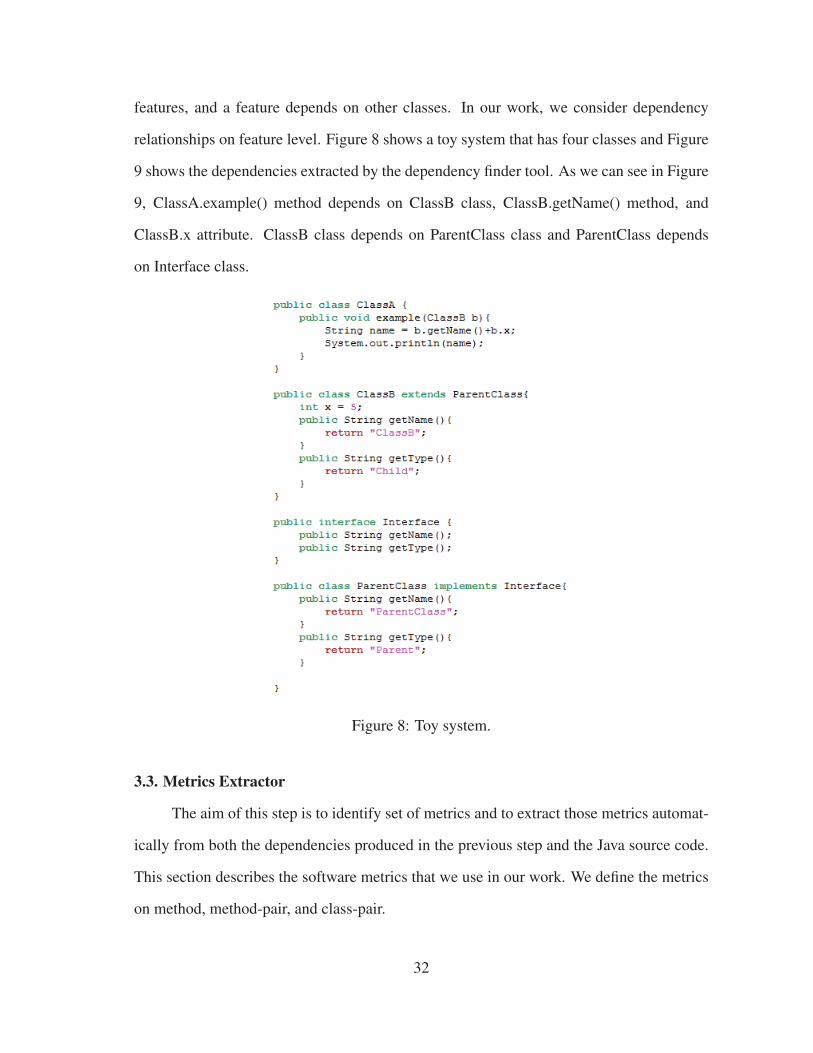
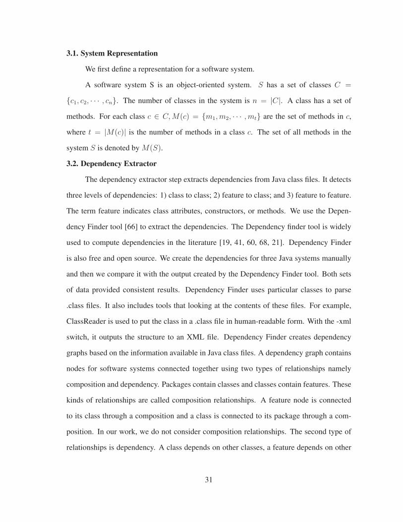
features, and a feature depends on other classes. In our work, we consider dependency
relationships on feature level. Figure 8 shows a toy system that has four classes and Figure
9 shows the dependencies extracted by the dependency finder tool. As we can see in Figure
9, ClassA.example() method depends on ClassB class, ClassB.getName() method, and
ClassB.x attribute. ClassB class depends on ParentClass class and ParentClass depends
on Interface class.
Figure 8: Toy system.
3.3. Metrics Extractor
The aim of this step is to identify set of metrics and to extract those metrics automat-
ically from both the dependencies produced in the previous step and the Java source code.
This section describes the software metrics that we use in our work. We define the metrics
on method, method-pair, and class-pair.
32
Figure 9: Dependencies of the toy system.
3.3.1. Method Level Metrics
We define metrics on individual methods within a class. For method mi in class
ci, most of these metrics calculate the number of classes, methods, and fields that have a
dependency with method mi. Figure 10 shows a simple Java example that will be used
to explain the method level metrics. The Java example contains two classes: MO class
and RO class. MO class contains two methods: getMin method and getMax method.
GetMin method returns the minimum value of any three numbers while getMax method
returns the maximum value of any three numbers. RO class contains the main method.
The main method creates an object from MO class. Figure 11 shows the coupling depen-
dency graph for the Java fragment of code. In Figure 11, the RO.main() method depends
on MO.magicNumber attribute, MO.getMin method, MO.getMax method, and MO.MO
constructor. In Figure 10, RO.main method calls the implicit constructor for MO class.
33
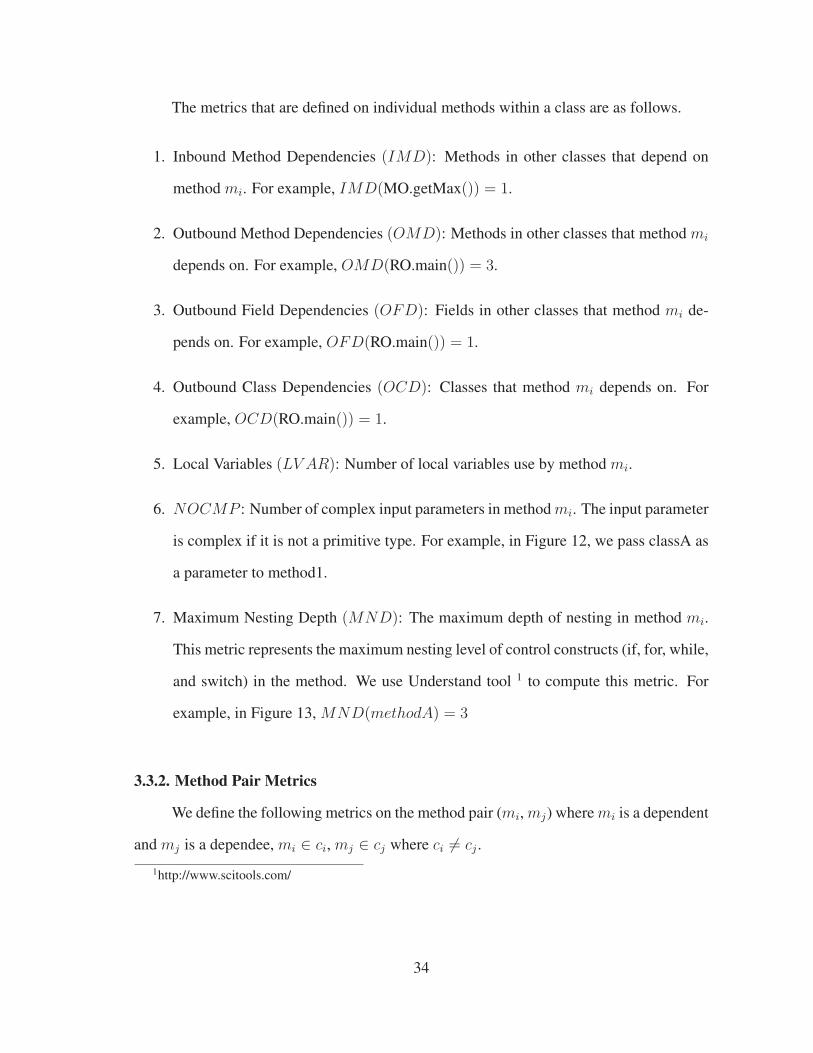
The metrics that are defined on individual methods within a class are as follows.
1. Inbound Method Dependencies (IMD): Methods in other classes that depend on
method mi. For example, IMD(MO.getMax()) = 1.
2. Outbound Method Dependencies (OMD): Methods in other classes that method mi
depends on. For example, OMD(RO.main()) = 3.
3. Outbound Field Dependencies (OFD): Fields in other classes that method mi de-
pends on. For example, OFD(RO.main()) = 1.
4. Outbound Class Dependencies (OCD): Classes that method mi depends on. For
example, OCD(RO.main()) = 1.
5. Local Variables (LV AR): Number of local variables use by method mi.
6. NOCMP : Number of complex input parameters in method mi. The input parameter
is complex if it is not a primitive type. For example, in Figure 12, we pass classA as
a parameter to method1.
7. Maximum Nesting Depth (MND): The maximum depth of nesting in method mi.
This metric represents the maximum nesting level of control constructs (if, for, while,
and switch) in the method. We use Understand tool 1 to compute this metric. For
example, in Figure 13, MND(methodA) = 3
3.3.2. Method Pair Metrics
We define the following metrics on the method pair (mi, mj) where mi is a dependent
and mj is a dependee, mi ∈ ci, mj ∈ cj where ci 6= cj .
1http://www.scitools.com/
34

1. Inbound Common Method Dependencies (ICMmimj): Number of common meth-
ods that depend on both mi and mj . In Figure 14, ICMm1m2 = 2 (m3 and m4
depend on both m1 and m2).
2. Outbound Common Method Dependencies (OCMmimj): Number of common meth-
ods that both mi and mj depends on. In Figure 15, OCMm1m2 = 1 (Both m1 and
m2 depend on m3.
3.4. Connections Ranker
In this step, We use combination of metrics defined in the previous step to rank the
connections between methods. The combination of metrics will be used to examine several
hypothesis regarding the correlation between these metrics and error discovery rate. The
rank of the connections specifies the connections that should be focused on during the
testing process.
For method-pair (mi,mj), the weight for the connection between mi and mj is calcu-
lated as follows:
weight(mi,mj) = (weight(mi) +weight(mj))× (ICMmimj +OCMmimj + 1) (2)
where weight(mi) is calculated as follows:
weight(mi|ck, cl) =ICmi
× (IMDmi +OMDmi +OFDmi)2
∑
y∈M(ck,cl)ICy × (IMDy +OMDy +OFDy)2
(3)
where M(ck, cl) is the set of methods in both class ck and class cl. ICmiis the internal
complexity of method mi. It can be measured as follows:
ICmi= MNDmi +NOCMPmi + LV ARmi (4)
35

3.5. Test Focus Selector
The Test focus selector step predicts the number of test cases needed to test each
connection based on the weights of the connections produced in the previous step and
given the initial minimum number of test cases needed. We would like to start with a small
initial number of test cases. In our work, we assume the initial number of test cases needed
to test a system S to be 0.10% of the number of interactions. After that, the number of
test cases can be adjusted depending on the error discovery rate. For example, if the initial
number of test cases to test a system was 50 and the error discovery rate was 60%, then
we generate and run 0.10% more test cases in each iteration until we reach 80% of error
discovery rate. The method-pair weight is computed using the equation in the previous
section. The class-pair weight is computed as the summation of all method-pair weights
that belong to the two classes. If the class-pair weight is zero, we specify one test case to
test the class-pair connection. Figure 16 explains the testing process used in our approach.
We start by creating w test cases where w is the initial number of test cases given by the
approach. We then run the test cases against the seeded versions of the applications and
we compute the error discovery rate. We stop if we achieve 80% error discovery rate.
Otherwise, we create more test cases (10% of the interactions in each iteration) until the
80% is achieved.
3.6. Generate Test Cases
In this step, test cases is created manually to test the required application. For
evaluating the testing process, both error seeding technique [47, 51] and mutation testing
are used. The test case generation step compares the original program with the seeded
program. If the test cases are enable to differentiate between the original program and the
seeded program, the seeded program is said to be killed; otherwise, it is still alive.
36
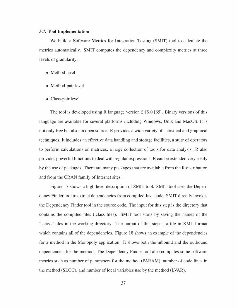
3.7. Tool Implementation
We build a Software Metrics for Integration Testing (SMIT) tool to calculate the
metrics automatically. SMIT computes the dependency and complexity metrics at three
levels of granularity:
• Method level
• Method-pair level
• Class-pair level
The tool is developed using R language version 2.15.0 [65]. Binary versions of this
language are available for several platforms including Windows, Unix and MacOS. It is
not only free but also an open source. R provides a wide variety of statistical and graphical
techniques. It includes an effective data handling and storage facilities, a suite of operators
to perform calculations on matrices, a large collection of tools for data analysis. R also
provides powerful functions to deal with regular expressions. R can be extended very easily
by the use of packages. There are many packages that are available from the R distribution
and from the CRAN family of Internet sites.
Figure 17 shows a high level description of SMIT tool. SMIT tool uses the Depen-
dency Finder tool to extract dependencies from compiled Java code. SMIT directly invokes
the Dependency Finder tool in the source code. The input for this step is the directory that
contains the compiled files (.class files). SMIT tool starts by saving the names of the
”.class” files in the working directory. The output of this step is a file in XML format
which contains all of the dependencies. Figure 18 shows an example of the dependencies
for a method in the Monopoly application. It shows both the inbound and the outbound
dependencies for the method. The Dependency Finder tool also computes some software
metrics such as number of parameters for the method (PARAM), number of code lines in
the method (SLOC), and number of local variables use by the method (LVAR).
37
Then, SMIT extracts all of the call graphs and saves the results in Call-Graphs Matrix
(CGM). We only consider calls between methods that belong to different classes. The
CGM matrix is a square binary t × t matrix, where t represents the number of methods in
the system. The matrix indicates the direct method invocation interactions. The value of
CGM[i,j] is defined as follows:
CGM [i, j] =
1 if the ith method invokes the jth method
0 otherwise
Where 1 ≤ i ≤ t and 1 ≤ j ≤ t. Rows of CGM matrix represent the callers
(dependents) where columns represent the callees (dependees). We exclude calls between
methods in the same class.
After extracting all of the call graphs, SMIT computes the method level metrics
namely NOCMP, IMD, OMD, and OFD. The NOCMP metric represents the number of
complex input parameters in a method where input parameter is considered complex if
it is not a primitive type (e.g., if it is of type class, array, or hashmap). Then, SMIT
computes method-pair metrics and computes a weight for each connection as discussed
in the connections ranker Section. After that, SMIT computes a weight for each class-pair.
A class-pair weight is computed as the summation of all method-pair weights that belong
to the two classes. Finally, SMIT predicts the number of test cases needed to test each
connection as explained in the test focus selector Section.
SMIT implementation program contains the following functions:
• classFiles(): It returns a list that contains the names of all class files (the files that
have the extension “.class”) in the working directory.
• extractDep(): This function extracts all of the dependencies for the system under test
using the DependencyFinder and it stores the the output in an XML file.
38

• callGraphs(): It extracts the call graphs for all methods in the system and it stores the
results in a matrix.
• inboundMethodCalls(mi): It returns all methods that depend on method mi.
• outboundMethodCalls(mi): It returns all methods that method mi depends on.
• outboundFeildDependencies(mi): It returns all fields that method mi depends on.
• lvarMetric(): It calculates the number of local variables used by a method.
• nocmpMetric(): It calculates the number of complex input parameters in a method.
• mndMetric(): It calculates the value of the MND metric for a method .
• icmMetric(): It calculates the value of the ICM metric for a method-pair.
• ocmMetric(): It calculates the value of the OCM metric for a method-pair.
• outboundMDep(): This function extracts the outbound method dependencies for a
method.
• inboundMDep(): This function extracts the inbound method dependencies for a method.
• weightmi(): This function calculates the weight for a method.
• weightmimj(): This function calculates the weight for a method-pair.
• classPairMetrics(): It computes the values of all class-pair metrics.
SMIT is provided with a command-line interface (CLI). Figure 19 shows an example
of running SMIT from the command line. It invokes the Rscript command which is
followed by the name of the program to be run (D:/javaSystems/smit.R ) and then followed
by an argument that specifies the working directory.
39

The outputs of our tool are four files in CSV format, method level metrics file,
method-pair level metrics file, class-pair level metrics file and a final report file. Figure
20 shows the output of SMIT and Figure 21 shows a screen capture for part of the final
report for the PureMVC application.
3.8. Toy Example
This section illustrates the proposed approach using a simple toy example. Figure 22
shows three classes and the dependencies between methods that belong to different classes.
For example, a directed arrow between m1 and m5 means that method m1 depends on
method m5. SMIT tool starts by computing the method-level metrics automatically from
both source code and byte code. Then, SMIT determines the method-pair interactions
such that the two methods should belong to different classes (i.e., we are not interested in
dependencies between methods in the same class). SMIT also calculates the method-pair
metrics. After that, the weight for each method pair is computed using Equation (2) and
the weight for each method is calculated using Equation (3). Figure 22 shows the weight
of each connection using toy numbers. For example, weight(m2,m6) = 0.81. SMIT
computes the the initial number of test cases which equals to 10% × No. of connections in
the system.
For the toy example in Figure 22, we assume that the initial number of test cases
is equal to 6. SMIT then computes the weight for each class pair as shown in Figure 23.
The class-pair weight is computed as the summation of all method-pair weights that belong
to the two classes. In Figure 22, weight(Class1, Class2) = 1.1 which equals to the
summation of the weights of the three method-pair (m1−m5, m2−m6, and m3−m7).
Table 1: The number of test cases needed to test class pairs.
Class-pair Weight Normalized Weight # of test cases
Class1 , Class2 1.1 0.453 0.453× 6 = ‖2.718‖ = 3Class1 , Class3 0.41 0.169 0.169× 6 = ‖1.014‖ = 1Class2 , Class3 0.92 0.379 0.379× 6 = ‖2.274‖ = 2
40

After that, SMIT computes the initial number of test cases needed to test each class-
pair as shown in Table 1. For example, the predicted number of test cases needed to test
class pair (class 1, class 2) is equal 3 and it is computed by multiplying the normalized
weight of the class-pair by the initial number of test cases and rounding the result to the
nearest integer. Finally, SMIT computes the initial number of test cases needed to test
each method-pair as shown in Table 2. For example, the predicted number of test cases
needed to test the method pair (m2, m6) is equal 2 and it is computed by multiplying the
normalized weight of the method-pair (0.736) by the initial number of test cases needed to
test the class-pair (3) and rounding the result to the nearest integer.
Table 2: The number of test cases needed to test method pairs.
Method-pair Weight Normalized Weight # of test cases
m1,m5 0.07 0.063 0.063× 3 = ‖0.189‖ = 0m2,m6 0.81 0.736 0.736× 3 = ‖2.208‖ = 2m3,m7 0.22 0.2 0.2× 3 = ‖0.6‖ = 1m4,m10 0.41 0.41 1m8,m11 0.73 0.793 0.793× 2 = ‖1.586‖ = 2m9,m12 0.19 0.206 0.206× 2 = ‖0.412‖ = 0
41

public class MO
{
public int magicNumber = 5000;
public double getMin( double x, double y, double z )
{
double minimum = x;
if ( y < minimum )
minimum = y;
if ( z < minimum )
minimum = z;
return minimum;
} // end method getMin
public double getMax( double x, double y, double z )
{
double maximum = x;
if ( y > maximum )
maximum = y;
if ( z > maximum )
maximum = z;
return maximum;
} // end method getMax
} // end class MO
public class RO
{
public double a = 5;
public double b = 3;
public double c = 1;
public void main()
{
MO mywork = new MO();
double w1 = mywork.getMin( a, b, c );
double w2 = mywork.getMax( a, b, c );
int m = mywork.magicNumber;
System.out.println(m);
} // end main
} // end class RO
Figure 10: Simple Java example that contains two classes MO and RO.
42
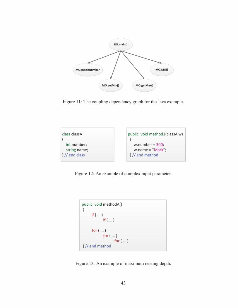
RO.main()
MO.magicNumber
MO.getMin() MO.getMax()
MO.MO()
Figure 11: The coupling dependency graph for the Java example.
class classA
{
int number;
string name;
} // end class
public void method1(classA w)
{
w.number = 300;
w.name = "Mark";
} // end method
Figure 12: An example of complex input parameter.
public void methodA()
{
if ( ... )
if ( ... )
for ( ... )
for ( ... )
for ( ... )
} // end method
Figure 13: An example of maximum nesting depth.
43
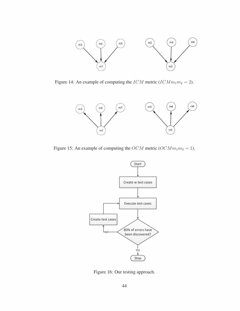
Figure 14: An example of computing the ICM metric (ICMm1m2 = 2).
Figure 15: An example of computing the OCM metric (OCMm1m2 = 1).
Start
Create w test cases
Execute test cases
80% of errors have
been discovered?
Stop
Create test cases
YES
NO
Figure 16: Our testing approach.
44

Source code Source codeClass files Class files
compile
Dependency
Finder tool
invoke
parse
CGM Matrix
extract call graphs
LVAR metric
Start
End
Understand
tool
MND metrics
Method-level
metrics
Class-pairs
weights
Connections
weights
Method-level
dependencies
Method-pair
metrics
All dependencies
Final Report
extract
Figure 17: High level description of SMIT tool.
45
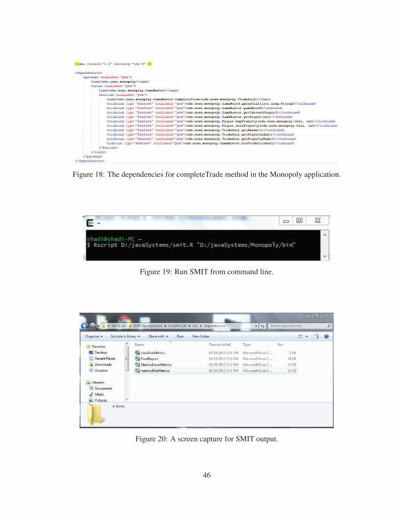
Figure 18: The dependencies for completeTrade method in the Monopoly application.
Figure 19: Run SMIT from command line.
Figure 20: A screen capture for SMIT output.
46
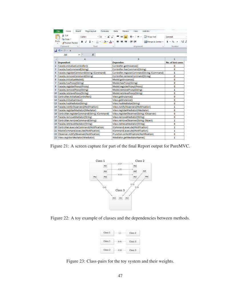
Figure 21: A screen capture for part of the final Report output for PureMVC.
Class 1
m1
m2
m3m4
Class 2
m5
m6
m7
m8
m9
Class 3
m10 m11 m12
0.07
0.81
0.22
0.41
0.73
0.19
Figure 22: A toy example of classes and the dependencies between methods.
Class 1 Class 21.1
Class 1 Class 30.41
Class 2 Class 30.92
Figure 23: Class-pairs for the toy system and their weights.
47

CHAPTER 4. EXPERIMENTAL EVALUATION
In order to evaluate the proposed approach, we select open-source applications im-
plemented in Java. Table 3 shows a summary of the selected applications. The selected
applications vary in size and domain and can be downloaded freely from the Internet. In
this chapter, we:
• describe the Java systems that we use in our evaluation
• present the results of the proposed approach
• discuss the results
Table 3: A summary of the selected applications.
Project # classes # methods Source
Monopoly 57 336 http://realsearchgroup.com/rose/
PureMVC 22 139 http://puremvc.org/
Cinema 10 106 http://alarcos.esi.uclm.es
ApacheCli 20 207 http://commons.apache.org/cli/
Pacman 25 208 http://code.google.com/p/stq-jpacman/
ApacheValidator 59 660 http://commons.apache.org/validator/
JTopas 63 753 http://sir.unl.edu
4.1. Selected Systems under Test
We select seven application in order to evaluate the proposed approach. We choose
these seven application to represent lots of domains. The two games applications (Monopoly
and Pacman) represent applications where systems have to interact a lot to satisfy the
logic rules of the underlying strategy of the game logic. The libraries and frameworks are
commonly used in Java where we usually strive for reusability in dependent applications.
We choose three libraries (ApacheCLI, ApacheValidator, and JTopas) to represent this
perspective. Since Java web-applications are widely used nowadays, we choose PureMVC
which implements the famous web design pattern Model-View-Controller (MVC). We
48

choose one business information system application (Cinema). A brief description of the
applications appears below.
4.1.1. Monopoly System
The Monopoly application presents a Monopoly-like computer game. Monopoly
provides many features that appear in the Monopoly board game. Many players play in
turns. A player moves based on the dice roll (two dices). When the user reaches the end
of the board, he/she cycles around. The system implements many rules of the Monopoly
game. For example, when a player passes or lands on the GO cell, the bank gives the player
200 dollars. Figure 24 shows the class diagram of the Monopoly system.
4.1.2. PureMVC
PureMVC is a light weight framework for creating applications based on the classic
Model, View and Controller concept. There are two versions of the PureMVC framework:
Standard and MultiCore. We use the standard Version that provides a methodology for
separating the coding interests according to the MVC concept. The application layers
are represented by three Singletons (a design pattern that limits the instantiation of a
class to one object). The MVC Singletons manage Proxies, Mediators and Commands.
Another Singleton, the Faade, provides a single interface for communications through the
application. Figure 25 shows the class diagram of the PureMVC system.
4.1.3. Cinema Management System
The Cinema application is an information management system. It is a movie theater
system that manages tickets booking, seats assignments, movie times, and movie locations.
This system is general enough to handle different types of theater halls such as VIP hall
and regular hall. Figure 26 shows the class diagram of the Cinema system.
49

::edu.ncsu.monopoly
MockTradeDialog
<<interface>>
RespondDialog
MockRespondDialog
<<interface>>
TradeDialogGameBoardUtility
SimpleGameBoardGameBoardRailRoad
GameBoardFull
GameBoardJail GoCell
GameBoardFreeParking
GoToJailCell CardCell
Cell
FreeParkingCell RailRoadCell
MockGUI
<<interface>>
MonopolyGUI
GameMaster
GameBoard
GameBoardCCLoseMoney
GameBoardCCMovePlayer
GameBoardCCGainMoney
GameBoardCCJail
GameBoard14
JailCard
Card
MoneyCard
MovePlayerCard
TradeDeal
Die
Player
PropertyCell
JailCell
UtilityCell
::edu.ncsu.monopoly.gui
<<interface>>
::<<Unknown>>::RespondDialog
::<<Unknown>>::JDialog
UtilDiceRoll
<<interface>>
CellInfoFormatter
RRCellInfoFormatter
CCCellInfoFormatterGoCellInfoFormatterGotoJailCellInfoFormatter
FreeParkingCellInfoFormatter
TestDiceRollDialogBuyHouseDialog
MainInfoFormatter
GameBoardUtil
GUITradeDialog
GUIRespondDialog
<<interface>>
::<<Unknown>>::TradeDialog
::<<Unknown>>::JPanel
GUICell InfoPanel
MainWindow
PlayerPanel
::<<Unknown>>::JFrame
<<interface>>
::<<Unknown>>::MonopolyGUI
JailCellInfoFormatter
UtilCellInfoFormatter
ChanceCellInfoFormatterPropertyCellInfoFormatter
Figure 24: The class diagram of Monopoly.
50

::org.puremvc.java.patterns.mediator
::org.puremvc.java.patterns.observer::Notifier
Mediator
<<interface>>
::org.puremvc.java.interfaces::IMediator
<<interface>>
::org.puremvc.java.interfaces::INotifier
::org.puremvc.java.patterns.observer
<<interface>>
::org.puremvc.java.interfaces::IObserver
<<interface>>
::org.puremvc.java.interfaces::IFunction
Observer
Notifier
::org.puremvc.java.patterns.facade::Facade<<interface>>
::org.puremvc.java.interfaces::INotification
Notification
::org.puremvc.java.core
<<interface>>
::org.puremvc.java.interfaces::IController
Controller
<<interface>>
::org.puremvc.java.interfaces::IView
View
<<interface>>
::org.puremvc.java.interfaces::IModel
Model
::org.puremvc.java.interfaces
<<interface>>
ICommand
<<interface>>
INotifier
<<interface>>
IModel<<interface>>
IView
<<interface>>
IProxy<<interface>>
IFacade
<<interface>>
IMediator
<<interface>>
IController<<interface>>
INotification
<<interface>>
IFunction<<interface>>
IObserver
::org.puremvc.java.patterns.command
::org.puremvc.java.patterns.observer::Notifier
MacroCommand SimpleCommand
<<interface>>
::org.puremvc.java.interfaces::ICommand
::org.puremvc.java.patterns.proxy
::org.puremvc.java.patterns.observer::Notifier
<<interface>>
::org.puremvc.java.interfaces::IProxy
Proxy
::org.puremvc.java.patterns.facade
::org.puremvc.java.core::Controller <<interface>>
::org.puremvc.java.interfaces::IFacade::org.puremvc.java.core::View ::org.puremvc.java.core::Model
Facade
Figure 25: The class diagram of PureMVC.
51

::dominio
AsientoCineSala
Sala_infantilSala_vip
Sesion
::dominio.exceptions
::<<Unknown>>::Exception
HoraExceptionSNException
FueradeloslimitesExceptionDniException
Figure 26: The class diagram of Cinema.
4.1.4. ApacheCli
The ApacheCli is a library that provides an API for parsing command line options
passed to programs. The library also can print help messages describing the available
options for a command line tool. For example, a boolean option is represented on a
command line by the presence of the option, i.e. the option value is true if the option
is found, otherwise the value is false. Figure 27 shows the class diagram of the ApacheCli
library.
4.1.5. Pacman System
The Pacman application simulates the arcade Pacman game. In this game, the player
controls Pac-Man through a maze, eating the dots. Pac-Man is taken to the next stage
when all dots are eaten. The Pacman system contains two packages namely controller and
model. An example of a class in this system is the Board class. The Board class maintains
52

::org.apache.commons.cli
Option CommandLineHelpFormatter.OptionComparatorOptionValidatorHelpFormatter
<<interface>>
::<<Unknown>>::Comparator
<<interface>>
::<<Unknown>>::Cloneable
<<interface>>
CommandLineParser
UnrecognizedOptionException BasicParserTypeHandler
Util OptionBuilder PatternOptionBuilder
PosixParser
Parser GnuParser
ParseException AlreadySelectedException
::<<Unknown>>::ExceptionMissingArgumentException
<<interface>>
::<<Unknown>>::Serializable
Options OptionGroup
MissingOptionException
Figure 27: The class diagram of the ApacheCLI.
a rectangular board of cells where guests can move around on the board, and keep track of
their position on the board. Figure 28 shows the class diagram of the Pacman system.
4.1.6. ApacheValidator
A major problem when receiving electronic data is verifying the integrity of the data.
This task becomes more complicated because different sets of validation rules need to be
applied to the same set of data. The ApacheValidator library tries to address this issue and
speed development and maintenance of validation rules. The ApacheValidator is a library
which provides validation for JavaBeans based on an XML file. This library also provides
standard validation routines and functions. It also provides reusable ”primitive” validation
methods. Figure 29 shows part of the class diagram of the ApacheValidator library.
4.1.7. JTopas
JTopas is used for parsing of arbitrary text data. These data can come from differ-
ent sources such as HTML, XML or RTF stream, source code of various programming
languages. JTopas classes provides many characteristics such as pattern matching and
whitespace handling. Figure 30 shows the class diagram of the JTopas library.
53

::jpacman.controller
Animator
BoardViewer
<<interface>>
::<<Unknown>>::Observer
AbstractMonsterController
<<interface>>
::<<Unknown>>::ActionListener
<<interface>>
IMonsterController
Pacman
RandomMonsterMover
::<<Unknown>>::JFrame
PacmanUI
<<interface>>
::<<Unknown>>::KeyListener
ImageFactory ::<<Unknown>>::JPanel
::jpacman.model
Game
GameLoader
Player
Monster
::<<Unknown>>::Exception
GameLoadException
::<<Unknown>>::Observable
Engine
Move
MonsterMove
PlayerMove
Board Cell Guest
Food
Wall
MovingGuest
Figure 28: The class diagram of Pacman.
54
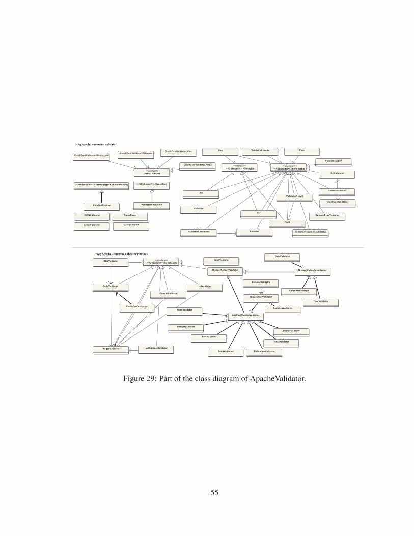
::org.apache.commons.validator
ISBNValidator NameBean
EmailValidator DateValidator
::<<Unknown>>::AbstractObjectCreationFactory
FormSetFactory
::<<Unknown>>::Exception
ValidatorException
Validator
<<interface>>
CreditCardType
CreditCardValidator.VisaCreditCardValidator.Discover
CreditCardValidator.Mastercard
CreditCardValidator.Amex
Arg
<<interface>>
::<<Unknown>>::Serializable
<<interface>>
::<<Unknown>>::Cloneable
Var
Msg ValidatorResults Form
ValidatorAction
UrlValidator
GenericValidator
CreditCardValidator
GenericTypeValidator
ValidatorResult
Field
ValidatorResult.ResultStatusFormSetValidatorResources
::org.apache.commons.validator.routines
IntegerValidator
ShortValidator
ISBNValidator
RegexValidator
CodeValidator
DomainValidator
CreditCardValidator
UrlValidator
BigDecimalValidator
PercentValidator
AbstractNumberValidator
DoubleValidator
FloatValidator
BigIntegerValidatorLongValidator
ByteValidator
<<interface>>
::<<Unknown>>::Serializable
AbstractFormatValidator
EmailValidator
InetAddressValidator
AbstractCalendarValidator
CurrencyValidator
DateValidator
CalendarValidator
TimeValidator
Figure 29: Part of the class diagram of ApacheValidator.
55

::org.puremvc.java.patterns.mediator
::org.puremvc.java.patterns.observer::Notifier
Mediator
<<interface>>
::org.puremvc.java.interfaces::IMediator
<<interface>>
::org.puremvc.java.interfaces::INotifier
::org.puremvc.java.patterns.observer
<<interface>>
::org.puremvc.java.interfaces::IObserver
<<interface>>
::org.puremvc.java.interfaces::IFunction
Observer
Notifier
::org.puremvc.java.patterns.facade::Facade<<interface>>
::org.puremvc.java.interfaces::INotification
Notification
::org.puremvc.java.core
<<interface>>
::org.puremvc.java.interfaces::IController
Controller
<<interface>>
::org.puremvc.java.interfaces::IView
View
<<interface>>
::org.puremvc.java.interfaces::IModel
Model
::org.puremvc.java.interfaces
<<interface>>
ICommand
<<interface>>
INotifier
<<interface>>
IModel<<interface>>
IView
<<interface>>
IProxy<<interface>>
IFacade
<<interface>>
IMediator
<<interface>>
IController<<interface>>
INotification
<<interface>>
IFunction<<interface>>
IObserver
::org.puremvc.java.patterns.command
::org.puremvc.java.patterns.observer::Notifier
MacroCommand SimpleCommand
<<interface>>
::org.puremvc.java.interfaces::ICommand
::org.puremvc.java.patterns.proxy
::org.puremvc.java.patterns.observer::Notifier
<<interface>>
::org.puremvc.java.interfaces::IProxy
Proxy
::org.puremvc.java.patterns.facade
::org.puremvc.java.core::Controller <<interface>>
::org.puremvc.java.interfaces::IFacade::org.puremvc.java.core::View ::org.puremvc.java.core::Model
Facade
Figure 30: The class diagram of JTopas.
56

4.2. JUnit Testing Framework
As mentioned in Chapter 3, SMIT tool predicts the number of test cases needed to test
each connection. We develop the test cases needed to test each system using JUnit testing
framework1. The JUnit framework is an open-source testing framework. JUnit is usually
used for developing unit tests where each single method is tested in isolation. In integration
testing, objects interact with each other in order to perform a task. Moreover, Objects in
medium and large size applications are very complex and they depend on external objects
to perform their tasks. For example, a method may need to access a database to perform
some tasks. Therefore, methods should be tested together and external objects should be
available in some way to simplify the testing process. A common technique for developing
integration test cases using JUnit is to create mock objects (mocks) that are used only
during running the test cases. A mock object, which is presented by Tim Mackinnon et al.
[44], is used to mimic a real-world object during testing.
Mocks are used to replace complex objects (e.g., databases, files, and internet con-
nection) that are needed by a method under test. One mock object is created for each real
object. Then, we can call a mock object in the test case. Mocks do not implement any
business logic and they are just dump objects driven by the tests. In other words, they are
empty skeletons that provide a mechanism to simulate the behavior of the faked class [4].
For example, in the Monopoly application, a mock object (mockGUI) is created
to simulate the Graphical User Interface (GUI) of the game. For each test suite that
needs to interact with the GUI, we provide the mock in the setup method of that test
suite (gameMaster.setGUI(new MockGUI())). Then, an object of that mock is created
inside the method in which the interaction with the GUI is needed (MonopolyGUI gui
= gameMaster.getGUI()).
1http://www.junit.org/
57

4.3. Experiments
In order to evaluate the proposed approach, we use both error seeding and mutation
analysis techniques. Section 4.3.1 presents the evaluation using error seeding and Section
4.3.4 presents the evaluation using mutation testing.
4.3.1. Error Seeding Testing
We gave error seeders a list that contains the most common integration errors as
categorized by Leung and White [38] and discussed by Orso [53]. We asked the error
seeders to inject different types of integration errors based on both the given integration
errors category and their experience. In order to get accurate results, applications are given
to three different third parties for error seeding and all results are included. The error
seeders have been asked to do the seeding independently to make the process as credible as
possible. Two types of error seeding experiments are used as follows:
• A number of seeded (faulty) programs are created for each application. Each seeded
program contains one error [32, 39]. Then, test cases are running against both the
original program and the seeded one. We say that the test cases detect the error if
they distinguish between the original program and the seeded one. Six Java appli-
cations are seeded by third party namely Monopoly, PureMVC, Cinema, ApacheCli,
Pacman, and ApacheValidator. In our work, error seeders are programmers with at
least three years of programming experience in Java.
• A combination of errors are injected into one version of the program to see the
effect of combining seeded errors in one faulty program on the effectiveness of our
proposed approach. This approach contains two variations as follows:
– Three faulty programs are created for each application by third party. The
programs are Pacman and Cinema. Each seeded program contains five errors.
58

– One faulty program is created for both PureMVC and JTopas. All integration
errors are injected in one faulty version. The number of injected faults is 15.
We run the minimum number of test cases for each system on both the original source
code of the system and the faulty versions of the system under test. We know the number of
inserted errors by the third party but we donot know the location of these errors. We check
that all test cases pass when they run against the original source code to make sure that the
test case detects the injected error when it fails while running against the faulty version.
4.3.2. Mutation Testing
We also applied mutation testing in order to further investigate the effectiveness
of our proposed approach. Previous work found that mutation testing is a reliable way
of assessing the fault-finding effectiveness of test cases and the generated mutants are
similar to real faults [5, 6]. We choose inter-class level mutation operators. Inter-class
level testing is usually applied when two or more classes are tested together to find inte-
gration faults [43]. Table 31 shows the mutation operator that we use in our work [43].
The set contains 24 mutation operators. Each mutation operator is related to one of the
six groups namely access control, inheritance, polymorphism, overloading, Java-specific
features, and common programming mistakes. The first four groups are common to all
object-oriented programming languages. Java-specific features group is exclusive for Java
programming language while the last group depends on common programming mistakes
in object-oriented languages. Mutants are usually created using an automated mutation
system. In our work, mutation operators are automatically generated using muJava tool 1.
MuJava tool is widely used to perform mutation analysis [71, 46]. After creating mutation
operators, test cases are running against both the original program and the faulty programs.
We say that the mutant is killed if test cases differentiate the output of the original program
from the mutant programs; otherwise the mutant is still alive.
1http://cs.gmu.edu/ offutt/mujava/
59

Figure 31: Mutation Operators for Inter-Class Testing.
4.3.3. Results of Error Seeding and Mutation
In this Section, we show the results of applying both error seeding and mutation
testing on the selected Java systems. For error seeding, the error detection rate is calculated
by dividing the number of detected seeded errors by the total number of seeded errors. For
mutation testing, the mutation score is calculated by dividing the number of killed mutants
by the total number of mutants.
Table 4: Error seeding results of the PureMVC application.
Source # of seeded errors Detected Not Detected Error detection rate
Third party A 19 16 3 84.21%
Third party B 10 8 2 80.00%
Third party C 15 13 2 86.67%
Table 4 shows the results of applying error seeding on the PureMVC application. For
the PureMVC application, 19 integration errors are inserted by third-party A and 16 of them
60

are detected. 10 integration errors are inserted by third-party B and 8 of them are detected.
15 integration errors are inserted by third-party C and 13 of them are detected. Table 5
shows the results of applying mutation testing on the PureMVC application. The number
of injected mutants is 51 and all of them are killed. Table 6 shows the results of applying
error seeding on the Cinema application. For the Cinema application, 20 integration errors
are inserted by third-party A and 17 of them are detected. 15 integration errors are inserted
by third-party B and C and 12 of them are detected. Table 7 shows the results of applying
mutation testing on the Cinema application. The number of injected mutants is 116 and all
of them are killed.
Table 5: Mutation testing results of the PureMVC application.
Application Class Live Killed Total Mutation score
PureMVC
Facade 0 10 10 100.00%Mediator 0 5 5 100.00%Notification 0 19 19 100.00%Notifier 0 11 11 100.00%Proxy 0 6 6 100.00%
Total 0 51 51 100.00%
Table 6: Error seeding results of the Cinema application.
Source # of seeded errors Detected Not Detected Error detection rate
Third party A 20 17 3 85.00%
Third party B 15 12 3 80.00%
Third party C 15 12 3 80.00%
Table 7: Mutation testing results of the Cinema application.
Application Class Live Killed Total Mutation score
Cinema
Asiento 0 6 6 100.00%Cine 0 94 94 100.00%Sesion 0 16 16 100.00%
Total 0 116 116 100.00%
61

Table 8 shows the results of applying error seeding on the ApacheCLI application.
For the ApacheCli application, 22 integration errors are inserted by third-party A and 19 of
them are detected. 15 integration errors are inserted by third-party B and 13 of them are
detected. 15 integration errors are inserted by third-party C and 12 of them are detected.
The number of injected mutants is 313 and all of them are killed.
Table 8: Error seeding results of the ApacheCLI application.
Source # of seeded errors Detected Not Detected Error detection rate
Third party A 22 19 3 86.36%
Third party B 15 13 2 86.67%
Third party C 15 12 3 80.00%
Table 10 shows the results of applying error seeding on the Pacman application. For
the Pacman application, 22 integration errors are inserted by third-part A and 18 of them
are detected. 15 integration errors are inserted by third-part B and 12 of them are detected.
15 integration errors are inserted by third-part C and 13 of them are detected.
Table 9: Mutation testing results of the ApacheCLI application.
Application Class Live Killed Total Mutation score
ApacheCLI
CommandLine 0 37 37 100.00%AlreadySelectedException 0 7 7 100.00%HelpFormatter 0 124 124 100.00%MissingArgumentException 0 6 6 100.00%MissingOptionException 0 1 1 100.00%Option 0 40 40 100.00%OptionBuilder 0 25 25 100.00%OptionGroup 0 39 39 100.00%Options 0 27 27 100.00%ParseException 0 1 1 100.00%PosixParser 0 4 4 100.00%TypeHandler 0 1 1 100.00%UnrecognizedPotionException 0 1 1 100.00%
Total 0 313 313 100.00%
62

Table 10: Error seeding results of the Pacman application.
Source # of seeded errors Detected Not Detected Error detection rate
Third party A 22 18 4 81.82%
Third party B 15 12 3 80.00%
Third party C 15 13 2 86.67%
Table 11: Error seeding results of the ApacheValidator application.
Source # of seeded errors Detected Not Detected Error detection rate
Third party A 24 21 3 87.50%
Third party B 15 13 2 86.67%
Third party C 15 13 2 86.67%
Table 11 shows the results of applying error seeding on the ApacheValidator applica-
tion. For the ApacheValidator application, 24 integration errors are inserted by third-party
A and 21 of them are detected in the first iteration. 15 integration errors are inserted by
third-party B and 8 of them are detected in the first iteration. Therefore, a second iteration
is performed to achieve at least 80% error detection rate. 13 errors out of 15 are detected in
the second iteration.
Table 12: Error seeding results of the Monopoly application.
Source # of seeded errors Detected Not Detected Error detection rate
Third party A 21 19 2 90.48%
Third party B 15 13 2 86.67%
Third party C 15 14 1 93.33%
Table 12 shows the results of applying error seeding on the Monopoly application.
For the Monopoly application, 21 integration errors are inserted by the third-party A and
19 of them are detected. 15 integration errors are inserted by the third-party B and 13 of
them are detected. 15 integration errors are inserted by the third-party C and 14 of them
are detected. Table 13 shows the results of applying mutation testing on the Monopoly
application. The number of injected mutants is 888 and all of them are killed.
63

We choose the JTopas application from Software-artifact Infrastructure Repository
(SIR) at University of Nebraska-lincoln 1. The JTopas application contains 63 classes,
753 methods, and 461 connections. We consider version 3 of the application where 16
seeded errors are available. We run SMIT tool on the JTopas application. SMIT suggests
writing 112 test cases. We develop the test cases using JUnit framework and we run the
test cases against the faulty version of the application. For the Jtpoas application,13 errors
are detected out of 16. The error detection rate is 81.25%.
Table 13: Mutation testing results of the Monopoly application.
Application Class Live Killed Total Mutation score
Monopoly
CardCell 0 1 1 100.00%
FreeParkingCell 0 1 1 100.00%
GameBoard 0 9 9 100.00%
GameBoard14 0 131 131 100.00%
GameBoardCCGainMoney 0 21 21 100.00%
GameBoardCCJail 0 21 21 100.00%
GameBoardCCLoseMoney 0 21 21 100.00%
GameBoardCCMovePlayer 0 21 21 100.00%
GameBoardFreeParking 0 1 1 100.00%
GameBoardFull 0 241 241 100.00%
GameBoardJail 0 51 51 100.00%
GameBoardRailRoad 0 41 41 100.00%
GameBoardUtility 0 41 41 100.00%
GameMaster 0 177 177 100.00%
GoToJailCell 0 1 1 100.00%
JailCard 0 2 2 100.00%
JailCell 0 2 2 100.00%
MockTradeDialog 0 2 2 100.00%
MoneyCard 0 6 6 100.00%
MovePlayerCard 0 3 3 100.00%
CellInfoFormatterTest 0 24 24 100.00%
PropertyCell 0 10 10 100.00%
RailRoadCell 0 4 4 100.00%
SimpleGameBoard 0 51 51 100.00%
TradeDeal 0 3 3 100.00%
UtilityCell 0 2 2 100.00%
Total 0 888 888 100.00%
1http://sir.unl.edu
64

It is worth pointing out that all of the selected systems achieve a detection rate higher
than 80% after the first iteration except for the ApacheValidator application seeded by third-
party B which achieves a detection rate higher than 80% after the second iteration.
Figure 32 shows the error detection rate for the applications under test where A
represents the programs seeded by third party A, B represents the programs seeded by
third party B, and C represents the programs seeded by third party C. Table 14 shows
the number of test cases developed to test each system. It also shows the percentage of
connections that are covered by the developed test cases. For example, in the Monopoly
application, we write 45 test cases to test 45 connections out of 449 connections and we
only cover 10.02% of the connections while detecting 90.48% of integration errors. The
Monopoly application achieves the highest reduction of the number of tested connections
(10.02%) while the PureMVC application achieves the lowest reduction (44.44%). For the
ApacheValidator, 72 test cases are developed for the first iteration. The error detection rate
for the system seeded by third-party B is 53.33%. Thus, a second iteration is performed by
adding 11 more test cases as recommended by SMIT.
70.00%
75.00%
80.00%
85.00%
90.00%
95.00%
A
B
C
Figure 32: Error detection rate for the selected applications.
65

Table 14: Number of test cases created for each application.
Project # of connections # of test cases Covered connections
Monopoly 449 45 10.02%
PureMVC 54 24 44.44%
Cinema 97 15 15.46%
ApcheCli 196 43 21.93%
Pacman 176 46 26.13%
ApacheValidator 275 72 26.18%
JTpoas 461 112 24.30%
4.3.4. Comparison with Related Work
Several approaches are found in the literature for defect prediction. These approaches
predict the probability that a file will have at least one error. Other approaches predict the
exact number of errors that may be found in a file where a file contains many classes. Most
of these approaches use complexity metrics as independent variables to predict the faulty
files. Zimmerman and Nagappan [72] mentioned that a main disadvantage of most com-
plexity metrics is that they only work on single files and they do not take the interactions
between different files in their considerations. On the same hand, these approaches can be
used for reducing the cost of unit testing by focusing the testing process on faulty files.
These approaches cannot be used for integration testing because they do not predict the
important interactions between files. In our work, we predict error-prone interactions and
we predict the number of test cases needed to test each one. A similar approach to ours is a
research by Borner and Paech [10]. In their work they presented an approach to select the
test focus in the integration test process. They identified correlations between dependency
properties and the number of errors in both the dependent and the independent files in the
previous versions of the system under test. They divided the test focus into four groups:
1) Not Test Focus, 2) Test Focus Dependent file, 3) Test Focus Independent File, and 4)
Test Focus Both Files. A dependency is assigned to the first group if it does not have any
error-prone property where a property is error prone if it correlates with the number of
66

errors in the dependent or independent file. A dependency is assigned to the second group
if it has at least one property that correlates with the number of errors in the dependent file.
A dependency is assigned to the third group if it has at least one property that correlates
with the number of errors in the independent file while a dependency is assigned to the last
group if it has at least one property that correlates with the number of errors in both files.
The main differences between our approach and Borner and Paech approach are:
• Their approach just works for systems that have previous versions while our approach
does not need previous versions of the system under test.
• Their approach predicts the error-prone dependencies while our approach not only
predicts the error-prone dependencies but also predicts the number of test cases
needed to test each dependency. In addition, we rank dependencies by giving a
weight for each dependency in which a dependency with a higher weight is assigned
more test cases than a dependency with a lower weight.
• They identify the correlations between the dependency properties and the number of
errors in the dependent and the independent file. In our work, we do not identify the
correlations between our metrics and the number of errors in files because we are
working on the method level and information about number of errors at the method
level is not available. In our view, identifying the correlations with the number of
errors in files is not an accurate measure because errors belong to different classes
inside the file and we cannot tell in which class the errors reside.
Previous integration testing approaches assume that all classes are not yet developed
when testing is started. Therefore, stubs and drivers are needed to simulate the function-
alities of the classes that are not been developed yet. The focus of these approaches is
to minimize the cost of testing by minimizing the number of stubs [16] or by minimizing
the overall stub complexity [2]. They achieve cost reduction by devising integration test
67

orders. In our work, we assume that all classes of the system under test are available when
the testing process is performed. Therefore, stubs and drivers are not needed in our case.
In addition, our focus is to reduce cost of integration testing by using small number of test
cases while detecting at least 80% of integration errors.
4.3.5. Comparison with the Base Line Approach
In this section, we are going to compare our proposed approach with a base line
approach. In our work, a base line approach is an approach in which all method-pair
connections should be tested. We assume that every connection needs only one test case.
We also assume that the base line approach will achieve 100% error detection rate because
writing integration test cases for all of the connections can be very time consuming. We
conduct two comparisons with the baseline approach. The first comparison is performed
by measuring the savings that can be obtained by our proposed approach. We measure the
percentage of test cases reduction using the following formula [58]:
Savings =|T | − |Tsmit|
|T |∗ 100 (5)
Where T is the number of test cases in the base line approach and Tsmit is the number
of test cases given by SMIT. The formula assumes that all test cases have uniform costs.
Table 15 measures the percentage of savings. It is clear from Table 15 that the minimum
percentage of savings is obtained for the PureMVC application (55.56) while the maximum
percentage of savings is obtained for the Monopoly application (89.98).
The second comparison is performed by computing a score which takes both error
detection rate and number of developed test cases in consideration. The score is computed
as follows:
Score =Error detection rate
Number of test cases(6)
68

Table 15: The percentage of savings.
Application Savings
Monopoly 89.98
PureMVC 55.56
Cinema 84.54
ApacheCli 78.06
Pacman 73.86
ApaValidator 73.81
JTopas 75.70
Table 16 shows the results of comparing our approach with the base line approach.
The results indicate that our proposed approach achieves a higher score than the base line
approach for all of the selected applications. We conclude that the proposed approach
outperforms the baseline approach for all of the applications.
Table 16: The results of comparing the proposed approach with the baseline approach.
ApplicationOur Approach The baseline Approach
# of test cases Detection score Score # of test cases Detection score Score
Monopoly 45 90.48% 2.01 449 100.00% 0.22
PureMVC 24 84.21% 3.51 54 100.00% 1.85
Cinema 15 85.00% 5.67 97 100.00% 1.03
ApacheCli 43 86.36% 2.01 196 100.00% 0.51
Pacman 46 80.00% 1.74 176 100.00% 0.57
ApacheValidator 72 87.50% 1.22 275 100.00% 0.36
JTopas 112 81.25% 0.73 461 100.00% 0.22
4.4. Discussion
As mentioned in the previous Section, we use both error seeding and mutation testing
techniques in order to evaluate the effectiveness of the proposed approach. We will start by
discussing the results of applying error seeding technique by three different third-parties
on six Java applications and JTpoas application which is seeded by SIR.
4.4.1. Applications Seeded by Third-party A
For the Monopoly system, 21 integration errors are seeded by a third party and 19
of them are detected by our developed test cases (45 test cases). The seeded errors are
69

distributed as follows: 9 wrong function errors are injected and 8 of them are detected, 3
extra function errors are injected and all of them are detected, 7 missing instructions are
injected and all of them are detected, 2 extra call instructions are injected and one of them
is detected using the developed test cases. The Monopoly system contains 57 classes and
449 connections where only 10.02% of the connections are covered by the developed test
cases while achieving 90.48% error detection rate. The results indicate that most of the
integration errors are exist in the top ranked 10% of the connections. This also proves
that our approach can predict effectively the important connections. In other words, the
connections that have higher weights are more important than the connections that have
lower weights.
For the PureMVC framework, 19 integration errors are injected, 16 of them are
detected by the developed test cases (24 test cases). The seeded errors are distributed as
follows: 8 wrong function errors are injected and 7 of them are detected, 2 extra function
errors are injected and one of them is detected, 8 missing instructions are injected and
7 of them are detected, 1 extra call instruction is injected and it is detected using the
developed test cases. PureMVC contains 22 classes and 54 connections where 44.44%
of the connections are covered by the developed test cases while achieving 84.21% error
detection rate. The results indicate that the PureMVC framework gives little reduction
of the number of covered connections (it covers 44.44% of the connections). One reason
that PureMVC covers more than 40% of the connections is that the number of connections
between classes is small (it contains 22 classes and 54 connections). Therefore, if we cover
only 10% of the connections, most of the class-pair connections will not be tested. Also,
in our approach, we specify at least one test case to test class-pair connections. Therefore,
we write test cases that cover most of the connections if the classes have few connections
between them. For the Cinema system, 20 integration errors are injected, 17 of them are
detected by the developed test cases (15 test cases). The seeded errors are distributed as
70

follows: 8 wrong function errors are injected and 7 of them are detected, 3 extra function
errors are injected and all of them are detected, 6 missing instructions are injected and 5 of
them are detected, 3 extra call instruction are injected and two of them are detected using
the developed test cases. The Cinema system contains 10 classes and 97 connections where
only 15.46% of the connections are covered by the developed test cases while achieving
85.00% error detection rate. The results indicate that 85% of errors exist in the top 15% of
connections. The Cinema system achieves the second highest reduction after the Monopoly
system.
For ApacheCLI, 22 integration errors are injected, 19 of them are detected by the
developed test cases (43 test cases). The seeded errors are distributed as follows: 7 wrong
function errors are injected and 6 of them are detected, 3 extra function errors are injected
and two of them are detected, 8 missing instructions are injected and 7 of them are detected,
4 extra call instruction are injected and all of them are detected using the developed test
cases. ApacheCLI contains 20 classes and 196 connections where 21.93% of the connec-
tions are covered by the developed test cases while achieving 86.36% error detection rate.
The results indicate that 86.36% of errors exist in the top 22% of connections.
For Pacman, 22 integration errors are injected, 18 of them are detected by the devel-
oped test cases (46 test cases). The seeded errors are distributed as follows: 8 wrong func-
tion errors are injected and 6 of them are detected, 2 extra function errors are injected and
one of them are detected, 7 missing instructions are injected and all of them are detected,
5 extra call instruction are injected and 4 of them are detected using the developed test
cases. Pacman contains 25 classes and 176 connections where 26.13% of the connections
are covered by the developed test cases while achieving 81.82% error detection rate in the
first iteration of the proposed approach. The approach starts with an initial number of test
cases that equals to 18 (10% of the connections). Then, the approach adds one test case to
cover the class-pair connections that have not been covered in the 10% of connections (i.e.,
71

the approach assigns at least one test case to cover each class-pair connection). The results
indicate that 81.82% of errors exist in the top 27% of connections. The Pacman system
achieves the lowest error detection rate.
For ApacheValidator, 24 integration errors are injected, 21 of them are detected by
the developed test cases (72 test cases). The seeded errors are distributed as follows: 11
wrong function errors are injected and all of them are detected, 4 extra function errors are
injected and two of them are detected, 5 missing instructions are injected and all of them are
detected, 4 extra call instruction are injected and 3 of them are detected using the developed
test cases. ApacheValidator contains 59 classes and 275 connections where 26.18% of the
connections are covered by the developed test cases while achieving 87.50% error detection
rate. The ApacheValidator library is the largest system in terms of the number of classes in
our experimental study and it’s detection rate exceeds 80% in the first iteration.
4.4.2. Applications Seeded by Third-party B
For the Monopoly system, 15 integration errors are seeded by a third party and 13 of
them are detected by our developed test cases. The seeded errors are distributed as follows:
10 interpretation errors are injected and 9 of them are detected, 5 miscoded call errors are
injected and 4 of them are detected. For PureMVC, 10 integration errors are seeded by a
third party and 8 of them are detected by our developed test cases. The seeded errors are
distributed as follows: 6 interpretation errors are injected and all of them are detected, 4
miscoded call errors are injected and 2 of them are detected. For Cinema, 15 integration
errors are seeded by a third party and 12 of them are detected by our developed test cases.
The seeded errors are distributed as follows: 6 interpretation errors are injected and 5 of
them are detected, 4 miscoded call errors are injected and all of them are detected, and 5
interface errors and 3 of them are detected. For ApacheCLI, 15 integration errors are seeded
by a third party and 13 of them are detected by our developed test cases. The seeded errors
are distributed as follows: 7 interpretation errors are injected and 5 of them are detected,
72

6 miscoded call errors are injected and all of them are detected, and 2 interface errors and
1 of them is detected. For Pacman, 15 integration errors are seeded by a third party and
12 of them are detected by our developed test cases. The seeded errors are distributed as
follows: 6 interpretation errors are injected and 4 of them are detected, 4 miscoded call
errors are injected and all of them are detected, and 5 interface errors and 4 of them are
detected. For ApacheValidator, 15 integration errors are seeded by a third party and 13 of
them are detected by our developed test cases. The seeded errors are distributed as follows:
9 interpretation errors are injected and 8 of them are detected, 2 miscoded call errors are
injected and 1 of them is detected, and 4 interface errors and 4 of them are detected.
4.4.3. Applications Seeded by Third-party C
For the Monopoly system, 15 integration errors are seeded by a third party and 14 of
them are detected by our developed test cases. The seeded errors are distributed as follows:
2 interpretation errors are injected and all of them are detected, 8 miscoded call errors are
injected and 7 of them are detected, and 5 interface errors and all of them are detected. For
PureMVC, 15 integration errors are seeded by a third party and 13 of them are detected
by our developed test cases. The seeded errors are distributed as follows: 1 interpretation
error is injected and it is detected, 13 miscoded call errors are injected and 12 of them are
detected, and 1 interface errors and it is not detected. For Cinema, 15 integration errors
are seeded by a third party and 12 of them are detected by our developed test cases. The
seeded errors are distributed as follows: 3 interpretation errors are injected and 1 of them
is detected, 8 miscoded call errors are injected and all of them are detected, and 4 interface
errors and 3 of them are detected.
For ApacheCLI, 15 integration errors are seeded by a third party and 12 of them
are detected by our developed test cases. The seeded errors are distributed as follows: 7
interpretation errors are injected and 6 of them are detected, 6 miscoded call errors are
injected and 4 of them are detected, and 2 interface errors and all of them are detected.
73

For Pacman, 15 integration errors are seeded by a third party and 13 of them are detected
by our developed test cases. The seeded errors are distributed as follows: 7 interpretation
errors are injected and all of them are detected, 4 miscoded call errors are injected and 3 of
them are detected, and 3 interface errors and 2 of them is detected. For ApacheValidator, 15
integration errors are seeded by a third party and 13 of them are detected by our developed
test cases. The seeded errors are distributed as follows: 5 interpretation errors are injected
and all of them are detected, 7 miscoded call errors are injected and 5 of them are detected,
and 3 interface errors and all of them are detected.
We also conduct an experiment where combination of errors are injected into one
version of the program to see the effect of combining seeded errors in one faulty program
on the effectiveness of our proposed approach. We select JTopas which contains 461
connections. The number of seeded errors is 16. For the Jtpoas application,13 errors are
detected out of 16. The error detection rate is 81.25% and we cover only 24.30% of the
connections. The results of JTopas indicates two main findings: 1) The effectiveness of the
proposed approach since we use another source of seeding errors other than the third party;
and 2) The proposed approach works well even when we combine all of the errors in one
version of the source code.
4.4.4. Mutation Testing
The second approach that we use to evaluate our approach is mutation testing. We
make the following observations based on the experimental results of mutation testing:
• For Monopoly, 888 inter-class mutations are injected and all of them are killed by
the developed test cases.
• For Cinema, 116 inter-class mutations are injected and all of them are killed by the
developed test cases.
• For ApacheCLI, 313 mutations are injected and all of them are killed.
74

• For PureMVC, 51 inter-class mutations are injected and all of them are killed by the
developed test cases.
The effectiveness of the proposed approach is confirmed by using error seeding and
mutation testing. The results of error seeding show that the developed test cases based on
SMIT detect at least 80% of integration errors. The mutation testing is performed using
mutation operators. The mutation operators focus on the integration aspects of Java to
support inter-class level testing [42]. The results of using mutation testing show that all of
the mutants are killed which serve as another evidence of the effectiveness of our proposed
approach. Therefore, our approach is effective in detecting most of the integration errors
by testing the highly ranked connections. The experimental results show that the highly
ranked connections contain most of the integration errors. It also shows SMIT reduces the
number of test cases needed for integration testing.
4.4.5. Threats to Validity
There are many reasons which limit the generality of the results of the proposed
approach. First, all of the considered systems are Java systems. Second, all of the selected
systems are open-source systems that may not represent all domains. Third, the selected
systems are not representative in terms of the number and sizes of classes. Therefore, large-
scale assessment is needed taking into account software systems from diverse domains,
implemented in different programming languages and environments in order to get more
general results.
75

CHAPTER 5. CONCLUSION AND FUTURE WORK
In this work, we proposed an approach to select the test focus in integration testing.
The goal is to reduce cost and time of integration testing through testing part of the con-
nections while still detecting at least 80% of integration errors. Our proposed approach is
divided into five steps. The first step is to extract the dependencies from the compiled Java
code. The dependencies will be used to extract the dependency metrics. The second step is
to extract the metrics automatically using both the source code and the dependencies from
the previous step. The output of this step is the metrics at different levels of granularity
which include method level metrics, method-pair metrics, and class-pair metrics. The third
step is to calculate a weight for each method-pair connection using combination of metrics
defined in the previous step. The fourth step is to predict the number of test cases needed to
test each method-pair connection based on the weights of the connections produced in the
previous step given the initial minimum number of test cases. The number of test cases can
be increased depending on the error discovery rate. The last step is to generate test cases
manually to test the designated application.
Some of the metrics used in this work are defined and selected to cover different
types of dependencies. We defined three method level dependency metrics namely Inbound
Method Dependencies (IMD), Outbound Method Dependencies (OMD), and Outbound
Field Dependencies (OFD). We defined two method-pair level dependency metrics namely
Inbound Common Method Dependencies (ICM) and Outbound Common Method Depen-
dencies (OCM). The other metrics are selected to cover the internal complexity of a method.
In our work, the internal complexity represented by three metrics namely Local Variables
(LVAR), Number of complex input parameters (NOCMP), and Maximum Nesting Depth
(MND).
We built SMIT tool using R language to calculate the metrics automatically and to
implement the proposed approach. The outputs of SMIT are four files in CSV format,
76

method metrics, method-pair metrics, class-pair, and a final report. The final report speci-
fies the number of test cases needed to test each connection.
We conducted experiments on several Java systems taken from different domains
which include two games systems, three Java libraries, one business application, and one
web application. To assess the effectiveness of our proposed approach, we used both error
seeding and mutation testing as follows:
• Manual integration errors were injected into the source code of the applications by
three third-parties to make sure that we get accurate results and solid conclusions.
• Automatic inter-class mutants were inserted into the source code by MuJava tool.
The effectiveness of the developed test cases based on SMIT recommendation was
evaluated using the following measures:
• Detection rate: The number of detected seeded errors divided by the number of all
seeded errors.
• Mutation score: The number of killed mutants divided by the number of all mutants.
• Savings: The percentage of test cases reduction.
• Score: The error detection rate divided by the number of developed test cases.
• Covered connections: The number of connections that we developed test cases for
divided by the number of all connections.
Our experimental evaluation using error seeding technique shows that the developed
test cases achieved error detection rate higher than or equal to 80.00% for all selected
systems in the first iteration except the ApacheValidator system which achieved an error
detection rate higher than 80% after the second iteration. Moreover, the results showed
77

that the PureMVC framework gave the lowest reduction of the number of covered con-
nections (44.44%) while the Monopoly system achieved the highest reduction (it covered
only 10.02% of the connections). Therefore, the experimental results showed that our
proposed approach is effective in selecting the test focus in integration testing. The small
number of developed test cases detected at least 80.00% of integration errors in all selected
applications. The proposed approach reduced the number of test cases needed by covering
only part of the connections. In addition, the results showed that at least 80% of integration
errors typically exist in the highly ranked connections, i.e., the highly ranked connections
have a higher probability to contain integration errors. Our experimental evaluation using
mutation testing shows that the developed test cases based on the proposed approach kill all
of the inter-class mutants which give another evidence on the effectiveness of our proposed
approach.
We compared our approach with the baseline approach. The comparison was per-
formed by calculating both the percentage of test cases reduction and the error detection
rate divided by the number of developed test cases. The results indicated that the proposed
approach outperformed the baseline approach for all applications. Therefore, our goal of
reducing time and cost of integration testing is achieved. One significant advantage of our
proposed approach is that almost all steps of our approach can be performed automatically.
In future, we want to select the test focus for integration testing using both method
level metrics and integration errors history of previous versions of the system under test.
Information about errors history can be obtained using bug tracking systems. All of the
dependency metrics for source code can be extracted automatically using SMIT tool. We
are planning to use previous versions of the system under test to identify the metrics that
correlate with the number of integration errors in the source code. The method level metrics
that have a high correlation with the number of integration errors will be used to select the
test focus of the new version of the system.
78

We are also planning to use our method level metrics to select the test focus for
unit testing. Our goal is to give a weight for each method in the system under test using
combination of dependency metrics and internal complexity metrics, and then we focus the
testing process on the highly ranked methods, i.e., methods that have higher weights. We
also want to predict the number of test cases needed to test each method in the system.
Future directions also include using textual coupling as another source of depen-
dencies. Textual coupling can be computed using the similarity between method-pairs.
Each method can be represented as a document and then information retrieval techniques
can be used to compute similarities between methods. We would like to investigate the
effect of using hybrid dependency metrics (our previous dependency metrics and the textual
coupling) on error detection rate.
In our work, we defined dependencies on method level. A finer grain level of depen-
dencies may improve the results. Therefore, we want to investigate the effect of defining
dependencies on statement level on the error detection rate. We are also planning to
define dependency metrics on the feature level. Different functionalities of a system can
be implemented as features. A feature contains many methods scattered over a system.
Feature level dependency metrics can be used to measure impact analysis where some
changes made to one feature usually have accidental results for other features resulting in
incorrect system behavior.
79

REFERENCES
[1] Aynur Abdurazik and Jeff Offutt, Using uml collaboration diagrams for static
checking and test generation, Proceedings of the 3rd international conference on The
unified modeling language: advancing the standard (Berlin, Heidelberg), UML’00,
Springer-Verlag, 2000, pp. 383–395.
[2] Aynur Abdurazik and Jeff Offutt, Using coupling-based weights for the class
integration and test order problem, vol. 52, Oxford University Press, August 2009,
pp. 557–570.
[3] Shaukat Ali, Lionel Briand, Muhammad Jaffar-ur Rehman, Hajra Asghar,
Muhammad Zohaib Iqbal, and Aamer Nadeem, A state-based approach to integration
testing based on uml models, Inf. Softw. Technol. 49 (2007), 1087–1106.
[4] Paul Ammann and Jeff Offutt, Introduction to software testing, Cambridge University
Press, 2008.
[5] James Andrews, Lionel Briand, and Yvan Labiche, Is mutation an appropriate tool
for testing experiments?[software testing], Software Engineering, 2005. ICSE 2005.
Proceedings. 27th International Conference on, IEEE, 2005, pp. 402–411.
[6] James Andrews, Lionel Briand, Yvan Labiche, and Akbar Siami Namin, Using
mutation analysis for assessing and comparing testing coverage criteria, Software
Engineering, IEEE Transactions on 32 (2006), no. 8, 608–624.
[7] Victor Basili, Lionel Briand, and Walcelio Melo, A validation of object-oriented
design metrics as quality indicators, IEEE Trans. Softw. Eng. 22 (1996), 751–761.
[8] Saıda Benlarbi and Walcelio Melo, Polymorphism measures for early risk prediction,
Proceedings of the 21st international conference on Software engineering (New York,
NY, USA), ICSE ’99, ACM, 1999, pp. 334–344.
[9] Lars Borner and Barbara Paech, Integration test order strategies to consider test
focus and simulation effort, Proceedings of the 2009 First International Conference
on Advances in System Testing and Validation Lifecycle (Washington, DC, USA),
VALID ’09, IEEE Computer Society, 2009, pp. 80–85.
[10] Lars Borner and Barbara Paech, Using dependency information to select the test focus
in the integration testing process, Proceedings of the 2009 Testing: Academic and
Industrial Conference - Practice and Research Techniques (Washington, DC, USA),
TAIC-PART ’09, IEEE Computer Society, 2009, pp. 135–143.
[11] Lionel Briand, Jie Feng, and Yvan Labiche, Using genetic algorithms and coupling
measures to devise optimal integration test orders, Proceedings of the 14th
international conference on Software engineering and knowledge engineering (New
York, NY, USA), SEKE ’02, ACM, 2002, pp. 43–50.
80
[12] Lionel Briand, Yvan Labiche, and Siyuan He, Automating regression test selection
based on uml designs, Inf. Softw. Technol. 51 (2009), 16–30.
[13] Lionel Briand, Yvan Labiche, and Yihong Wang, Revisiting strategies for ordering
class integration testing in the presence of dependency cycles, Proceedings of the
12th International Symposium on Software Reliability Engineering (Washington, DC,
USA), ISSRE ’01, IEEE Computer Society, 2001.
[14] Lionel Briand, Jurgen Wust, John Daly, and Victor Porter, Exploring the relationship
between design measures and software quality in object-oriented systems, J. Syst.
Softw. 51 (2000), 245–273.
[15] Lionel Briand, Jurgen Wust, and Hakim Lounis, Replicated case studies
for investigating quality factors in object-oriented designs, Empirical Software
Engineering: An International Journal 6 (2001), 11–58.
[16] Lionel C Briand, Yvan Labiche, and Yihong Wang, An investigation of graph-based
class integration test order strategies, Software Engineering, IEEE Transactions on
29 (2003), no. 7, 594–607.
[17] Philippe Chevalley, Applying mutation analysis for object-oriented programs using a
reflective approach, Proceedings of the Eighth Asia-Pacific on Software Engineering
Conference (Washington, DC, USA), APSEC ’01, IEEE Computer Society, 2001,
pp. 267–.
[18] Shyam Chidamber and Chris Kemerer, A metrics suite for object oriented design,
IEEE Transactions on Software Engineering 20 (1994), 476–493.
[19] Peter Clarke, Djuradj Babich, Tariq King, and BM Golam Kibria, Analyzing clusters
of class characteristics in oo applications, J. Syst. Softw. 81 (2008), 2269–2286.
[20] Richard DeMillo, Richard Lipton, and Frederick Sayward, Hints on test data
selection: Help for the practicing programmer, Computer 11 (1978), 34–41.
[21] Jens Dietrich, Catherine McCartin, Ewan Tempero, and Syed Ali Shah, On
the existence of high-impact refactoring opportunities in programs, Australasian
Computer Science Conference (ACSC 2012) (Melbourne, Australia) (M. Reynolds
and B Thomas, eds.), CRPIT, vol. 122, ACS, 2012, pp. 37–48.
[22] Sebastian Elbaum, Alexey Malishevsky, and Gregg Rothermel, Incorporating varying
test costs and fault severities into test case prioritization, ICSE, 2001, pp. 329–338.
[23] Sebastian Elbaum, Alexey Malishevsky, and Gregg Rothermel, Test case
prioritization: A family of empirical studies, Software Engineering, IEEE
Transactions on 28 (2002), no. 2, 159–182.
81
[24] Khaled El Emam, Walcelio Melo, and Javam Machado, The prediction of faulty
classes using object-oriented design metrics, Journal of Systems and Software 56
(2001), 63–75.
[25] Jeanne Ferrante, Karl Ottenstein, and Joe Warren, The program dependence graph
and its use in optimization, ACM Transactions on Programming Languages and
Systems (TOPLAS) 9 (1987), no. 3, 319–349.
[26] Falk Fraikin and Thomas Leonhardt, Seditec ” testing based on sequence diagrams,
Proceedings of the 17th IEEE international conference on Automated software
engineering (Washington, DC, USA), ASE ’02, IEEE Computer Society, 2002,
pp. 261–.
[27] Leonard Gallagher, Jeff Offutt, and Anthony Cincotta, Integration testing of object-
oriented components using finite state machines: Research articles, Softw. Test. Verif.
Reliab. 16 (2006), 215–266.
[28] Todd Graves, Mary Jean Harrold, Jung-Min Kim, Adam Porter, and Gregg Rothermel,
An empirical study of regression test selection techniques, (1998), 188–197.
[29] Vu Le Hanh, Kamel Akif, Yves Le Traon, and Jean-Marc Jezequel, Selecting
an efficient oo integration testing strategy: An experimental comparison of actual
strategies, Proceedings of the 15th European Conference on Object-Oriented
Programming (London, UK, UK), ECOOP ’01, Springer-Verlag, 2001, pp. 381–401.
[30] Bill Hetzel, The complete guide to software testing, 2nd ed., QED Information
Sciences, Inc., Wellesley, MA, USA, 1988.
[31] Rattikorn Hewett, Phongphun Kijsanayothin, and Darunee Smavatkul, Test order
generation for efficient object-oriented class integration testing., SEKE, Knowledge
Systems Institute Graduate School, 2008, pp. 703–708.
[32] Monica Hutchins, Herb Foster, Tarak Goradia, and Thomas Ostrand, Experiments
of the effectiveness of dataflow- and controlflow-based test adequacy criteria,
Proceedings of the 16th international conference on Software engineering, ICSE ’94,
IEEE Computer Society Press, 1994, pp. 191–200.
[33] Zhenyi Jin and Jefferson Offutt, Coupling-based criteria for integration testing,
Software Testing Verification and Reliability 8 (1998), no. 3, 133–154.
[34] Sunwoo Kim, John A Clark, and John A McDermid, Class mutation: Mutation testing
for object-oriented programs, Proc. Net. ObjectDays, Citeseer, 2000, pp. 9–12.
[35] Bogdan Korel, The program dependence graph in static program testing, Inf. Process.
Lett. 24 (1987), 103–108.
[36] Gilbert Thomas Laycock and Gilbert Thomas Laycock, The theory and practice of
specification based software testing, Tech. report, Sheffield University, 1993.
82

[37] YS Lee, BS Liang, SF Wu, and FJ Wang, Measuring the coupling and cohesion of an
object-oriented program based on information flow, Proc. International Conference
on Software Quality, Maribor, Slovenia, 1995, pp. 81–90.
[38] Hareton KN Leung and Lee White, A study of integration testing and software
regression at the integration level, Software Maintenance, 1990., Proceedings.,
Conference on, IEEE, 1990, pp. 290–301.
[39] Nan Li, Upsorn Praphamontripong, and Jeff Offutt, An experimental comparison
of four unit test criteria: Mutation, edge-pair, all-uses and prime path coverage,
Software Testing, Verification and Validation Workshops, 2009. ICSTW’09.
International Conference on, IEEE, 2009, pp. 220–229.
[40] Wei Li and Sallie Henry, Object-oriented metrics that predict maintainability, Journal
of systems and software 23 (1993), no. 2, 111–122.
[41] Rdiger Lincke, Jonas Lundberg, and Welf Lwe, Comparing software metrics tools.,
ISSTA (Barbara G. Ryder and Andreas Zeller, eds.), ACM, 2008, pp. 131–142.
[42] Yu-Seung Ma, Yong-Rae Kwon, and Jeff Offutt, Inter-class mutation operators
for java, Proceedings of the 13th International Symposium on Software Reliability
Engineering (Washington, DC, USA), ISSRE ’02, IEEE Computer Society, 2002,
pp. 352–360.
[43] Yu-Seung Ma, Jeff Offutt, and Yong Rae Kwon, Mujava: an automated class
mutation system: Research articles, Softw. Test. Verif. Reliab. 15 (2005), 97–133.
[44] Tim Mackinnon, Steve Freeman, and Philip Craig, Extreme programming examined,
(2001), 287–301.
[45] Robert Martin, Oo design quality metrics - an analysis of dependencies, Workshop
Pragmatic and Theoretical Directions in Object-Oriented Software Metrics, 1994.
[46] Ammar Masood, Rafae Bhatti, Arif Ghafoor, and Aditya P. Mathur, Scalable and
effective test generation for role-based access control systems, IEEE Trans. Softw.
Eng. 35 (2009), 654–668.
[47] HD Mills, On the statistical validation of computer programs, IBM Federal Syst. Div.,
Tech. Rep (1972), 72–6015.
[48] Larry Morell, A theory of fault-based testing, Software Engineering, IEEE
Transactions on 16 (1990), no. 8, 844–857.
[49] Glenford Myers, Corey Sandler, and Tom Badgett, The art of software testing, Wiley,
2011.
83

[50] Nachiappan Nagappan and Thomas Ball, Using software dependencies and churn
metrics to predict field failures: An empirical case study, Proceedings of the First
International Symposium on Empirical Software Engineering and Measurement
(Washington, DC, USA), ESEM ’07, IEEE Computer Society, 2007, pp. 364–373.
[51] Jefferson Offutt and Huffman Hayes, A semantic model of program faults, ACM
SIGSOFT Software Engineering Notes, vol. 21, ACM, 1996, pp. 195–200.
[52] Jefferson Offutt, Roy Pargas, Scott Fichter, and Prashant Khambekar, Mutation
testing of software using a mimd computer, in 1992 International Conference on
Parallel Processing, Citeseer, 1992.
[53] Alessandro Orso, Integration testing of object-oriented software, Ph.D. thesis,
Politecnico di Milano, Milan, Italy, february 1999.
[54] Alessandro Orso, Saurabh Sinha, and Mary Jean Harrold, Classifying data
dependences in the presence of pointers for program comprehension, testing, and
debugging, ACM Trans. Softw. Eng. Methodol. 13 (2004), 199–239.
[55] Shari Lawrence Pfleeger, Software engineering: Theory and practice, 2nd ed.,
Prentice Hall PTR, Upper Saddle River, NJ, USA, 2001.
[56] Andy Podgurski and Lori A. Clarke, A formal model of program dependences
and its implications for software testing, debugging, and maintenance, Software
Engineering, IEEE Transactions on 16 (1990), no. 9, 965–979.
[57] Jane Radatz, Anne Geraci, and Freny Katki, Ieee standard glossary of software
engineering terminology, vol. 610121990, 1990.
[58] Gregg Rothermel, Mary Jean Harrold, Jeffery Ostrin, and Christie Hong, An empirical
study of the effects of minimization on the fault detection capabilities of test suites, In
Proceedings of the International Conference on Software Maintenance, 1998, pp. 34–
43.
[59] Adrian Schroter, Thomas Zimmermann, and Andreas Zeller, Predicting component
failures at design time, Proceedings of the 2006 ACM/IEEE international symposium
on Empirical software engineering, ISESE ’06, ACM, 2006, pp. 18–27.
[60] Alexander Serebrenik, Serguei Roubtsov, and Mark van den Brand, Dn-
based architecture assessment of java open source software systems, Program
Comprehension, 2009. ICPC’09. IEEE 17th International Conference on, IEEE, 2009,
pp. 198–207.
[61] Saurabh Sinha, Mary Jean Harrold, and Gregg Rothermel, Interprocedural control
dependence, ACM Trans. Softw. Eng. Methodol. 10 (2001), 209–254.
84

[62] Arthur G Stephenson, Daniel R Mulville, Frank H Bauer, Greg A Dukeman, Peter
Norvig, LS LaPiana, PJ Rutledge, D Folta, and R Sackheim, Mars climate orbiter
mishap investigation board phase i report, 44 pp, NASA, Washington, DC (1999).
[63] Sriraman Tallam and Neelam Gupta, A concept analysis inspired greedy algorithm for
test suite minimization, ACM SIGSOFT Software Engineering Notes, vol. 31, ACM,
2005, pp. 35–42.
[64] Gregory Tassey, The economic impacts of inadequate infrastructure for software
testing, Tech. report, 2002.
[65] RDevelopment Core Team, R: A language and environment for statistical computing.
vienna, austria: R foundation for statistical computing; 2008, 2011.
[66] Jean Tessier, Dependency finder, URL http://depfind. sourceforge. net/. Zugriffsdatum
4 (2010).
[67] Nancy J Wahl, An overview of regression testing, ACM SIGSOFT Software
Engineering Notes 24 (1999), no. 1, 69–73.
[68] Wei Wang, Xuan Ding, Chunping Li, and Hui Wang, A Novel Evaluation Method for
Defect Prediction in Software Systems, International Conference on Computational
Intelligence and Software Engineering (Wuhan, China), 2010, pp. 1–5.
[69] Zhengshan Wang, Bixin Li, Lulu Wang, Meng Wang, and Xufang Gong,
Using coupling measure technique and random iterative algorithm for inter-
class integration test order problem, Proceedings of the 2010 IEEE 34th Annual
Computer Software and Applications Conference Workshops (Washington, DC,
USA), COMPSACW ’10, IEEE Computer Society, 2010, pp. 329–334.
[70] Norman Wilde, Understanding program dependencies, Citeseer, 1990.
[71] Bo Yu, Liang Kong, Yufeng Zhang, and Hong Zhu, Testing java components based
on algebraic specifications, Proceedings of the 2008 International Conference on
Software Testing, Verification, and Validation (Washington, DC, USA), ICST ’08,
IEEE Computer Society, 2008, pp. 190–199.
[72] Thomas Zimmermann and Nachiappan Nagappan, Predicting defects using network
analysis on dependency graphs, Proceedings of the 30th international conference on
Software engineering (New York, NY, USA), ICSE ’08, ACM, 2008, pp. 531–540.
[73] Thomas Zimmermann and Nachiappan Nagappan, Predicting defects with program
dependencies (short paper), Proceedings of the Third International Symposium on
Empirical Software Engineering and Measurement, October 2009.
85
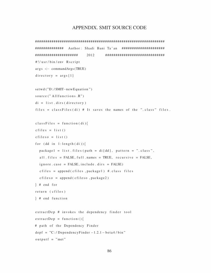
APPENDIX. SMIT SOURCE CODE
###############################################################
############## Author : Shad i Bani Ta ’ an #####################
##################### 2012 #############################
# ! / u s r / b i n / env R s c r i p t
a r g s <− commandArgs (TRUE)
d i r e c t o r y = a r g s [ 1 ]
se twd ( ”D : / SMIT−newEquat ion ” )
s o u r c e ( ” A l l f u n c t i o n s . R” )
d i = l i s t . d i r s ( d i r e c t o r y )
f i l e s = c l a s s F i l e s ( d i ) # I t s a v e s t h e names o f t h e ” . c l a s s ” f i l e s .
c l a s s F i l e s = f u n c t i o n ( d i ){
c f i l e s = l i s t ( )
c f i l e s o = l i s t ( )
f o r ( dd i n 1 : l e n g t h ( d i ) ) {
package1 = l i s t . f i l e s ( p a t h = d i [ dd ] , p a t t e r n = ” . c l a s s ” ,
a l l . f i l e s = FALSE , f u l l . names = TRUE, r e c u r s i v e = FALSE ,
i g n o r e . c a s e = FALSE , i n c l u d e . d i r s = FALSE)
c f i l e s = append ( c f i l e s , package1 ) # . c l a s s f i l e s
c f i l e s o = append ( c f i l e s o , package2 )
} # end f o r
r e t u r n ( c f i l e s )
} # end f u n c t i o n
e x t r a c t D e p # i n v o k e s t h e dependency f i n d e r t o o l
e x t r a c t D e p = f u n c t i o n ( ) {
# p a t h o f t h e Dependency F i n d e r
dep f = ”C : / DependencyFinder −1.2.1− b e t a 4 / b i n ”
o u t p u t f = ” met ”
86
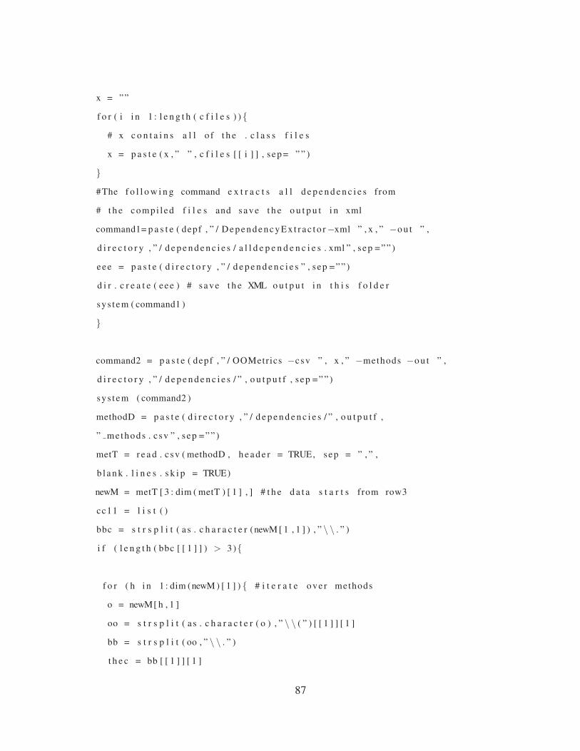
x = ””
f o r ( i i n 1 : l e n g t h ( c f i l e s ) ) {
# x c o n t a i n s a l l o f t h e . c l a s s f i l e s
x = p a s t e ( x , ” ” , c f i l e s [ [ i ] ] , sep = ” ” )
}
#The f o l l o w i n g command e x t r a c t s a l l d e p e n d e n c i e s from
# t h e compi l ed f i l e s and save t h e o u t p u t i n xml
command1= p a s t e ( depf , ” / D e p e n d e n c y E x t r a c t o r−xml ” , x , ” −o u t ” ,
d i r e c t o r y , ” / d e p e n d e n c i e s / a l l d e p e n d e n c i e s . xml ” , sep =”” )
eee = p a s t e ( d i r e c t o r y , ” / d e p e n d e n c i e s ” , sep =”” )
d i r . c r e a t e ( eee ) # s ave t h e XML o u t p u t i n t h i s f o l d e r
sys tem ( command1 )
}
command2 = p a s t e ( depf , ” / OOMetrics −csv ” , x , ” −methods −o u t ” ,
d i r e c t o r y , ” / d e p e n d e n c i e s / ” , o u t p u t f , sep =”” )
sys tem ( command2 )
methodD = p a s t e ( d i r e c t o r y , ” / d e p e n d e n c i e s / ” , o u t p u t f ,
” methods . csv ” , sep =”” )
metT = r e a d . csv ( methodD , h e a d e r = TRUE, sep = ” , ” ,
b l a n k . l i n e s . s k i p = TRUE)
newM = metT [ 3 : dim ( metT ) [ 1 ] , ] # t h e d a t a s t a r t s from row3
cc11 = l i s t ( )
bbc = s t r s p l i t ( a s . c h a r a c t e r (newM [ 1 , 1 ] ) , ” \ \ . ” )
i f ( l e n g t h ( bbc [ [ 1 ] ] ) > 3){
f o r ( h i n 1 : dim (newM ) [ 1 ] ) { # i t e r a t e ov e r methods
o = newM[ h , 1 ]
oo = s t r s p l i t ( a s . c h a r a c t e r ( o ) , ” \ \ ( ” ) [ [ 1 ] ] [ 1 ]
bb = s t r s p l i t ( oo , ” \ \ . ” )
t h e c = bb [ [ 1 ] ] [ 1 ]
87

f o r ( hh i n 3 : l e n g t h ( bb [ [ 1 ] ] ) −1 ){
t h e c = p a s t e ( thec , ” . ” , bb [ [ 1 ] ] [ hh ] , sep =”” )
}# end f o r hh
cc11 = append ( cc11 , t h e c )
} # end f o r h
cc11 = u n iq ue ( cc11 )
} # end i f
############
myM = l v a r M e t r i c (newM)
l v a r M e t r i c = f u n c t i o n (newM){
myM = newM[ , c ( 1 , 6 ) ] # methodName , Loca l V a r i a b l e s
r e t u r n (myM)
}
rn = as . m a t r i x (newM [ , 1 ] )
row . names (newM) = rn
mmm = m a t r i x ( 0 , l e n g t h ( rn ) , l e n g t h ( rn ) ) # CGM M at r ix
row . names (mmm) = rn
colnames (mmm) = rn
C L i s t = l i s t ( ) # s ave c l a s s e s names i n C L i s t
f o r ( s s i n 1 : l e n g t h ( c f i l e s ) ) {
#m1 c a l l s omethod and t h e y a r e i n d i f f e r e n t c l a s s e s
C L i s t = append ( CLis t , s t r s p l i t ( c f i l e s [ [ s s ] ] , ” \ \ . ” ) [ [ 1 ] ] [ 1 ] )
}
# E x t r a c t C a l l Graphs
# We on ly c o n s i d e r c a l l s be tween methods i n d i f f e r e n t c l a s s e s
n1 = p a s t e ( d i r e c t o r y , ” / d e p e n d e n c i e s / method ” , sep =”” )
# c r e a t e f o l d e r t o save d e p e n d e n c i e s f o r each method
d i r . c r e a t e ( n1 )
f o r ( j i n 1 : l e n g t h ( rn ) ) {
m1 = rn [ j ] # example
88

i f ( s u b s t r (m1 , n c h a r (m1 ) , n c h a r (m1 ) ) != ” ) ” ) {
n e x t
}
m2 = s t r s p l i t (m1 , ” \ \ ( ” ) [ [ 1 ] ] [ 1 ]
command3 = p a s t e ( depf , ” / DependencyRepor t e r −xml −o u t ” ,
d i r e c t o r y , ” / d e p e n d e n c i e s / method /M−” ,m2 , ” . xml − f 2 f ” ,
d i r e c t o r y , ” / d e p e n d e n c i e s / a l l d e p e n d e n c i e s . xml
−f e a t u r e −scope−i n c l u d e s / ” , m2 , ” / ” , sep =”” )
sys tem ( command3 )
} # end f o r j
mmm = c a l l G r a p h s ( rn )
c a l l G r a p h s = f u n c t i o n ( rn ){
f o r ( i i n 1 : l e n g t h ( rn ) ) {
m1 = rn [ i ]
m o r i g i n a l 1 = rn [ i ]
i f ( s u b s t r (m1 , n c h a r (m1 ) , n c h a r (m1 ) ) != ” ) ” ) {
n e x t
}
m2 = s t r s p l i t (m1 , ” \ \ ( ” ) [ [ 1 ] ] [ 1 ]
name = p a s t e ( d i r e c t o r y , ” / d e p e n d e n c i e s / method /M−” ,
m2 , ” . xml ” , sep =”” )
aaa1 = s t r s p l i t (m1 , ” \ \ ( ” ) [ [ 1 ] ]
ana11 = gsub ( ” . ” , ” : ” , aaa1 [ 2 ] , f i x e d =TRUE)
m1 = p a s t e ( aaa1 [ 1 ] , ” ( ” , ana11 , sep =”” )
moutbound = r e a d L i n e s ( name )
ou = ””
oumm = ””
ou = grep (”< outbound ” , moutbound , v a l u e =TRUE)
oumm = grep ( ” ) ” , ou , v a l u e =TRUE)
i f ( l e n g t h (oumm) > 0) {
89

f o r ( j i n 1 : l e n g t h (oumm ) ) { # a l l ou tbound d e p e n d e n c i e s
t e x = oumm[ j ]
p1 = s t r s p l i t ( t ex ,” >”)
omethod = s t r s p l i t ( p1 [ [ 1 ] ] [ 2 ] , ” < ” ) [ [ 1 ] ] [ 1 ]
i f ( omethod %i n% rn ){
s t r c = s t r s p l i t ( omethod , ” \ \ . ” )
c lassName = s t r s p l i t ( omethod , ” \ \ . ” ) [ [ 1 ] ] [ l e n g t h ( s t r c [ [ 1 ] ] ) −1 ]
s t r c m = s t r s p l i t (m1 , ” \ \ . ” )
c lassName2 = s t r s p l i t (m1 , ” \ \ . ” ) [ [ 1 ] ] [ l e n g t h ( s t r c m [ [ 1 ] ] ) −1 ]
i f ( c lassName != className2 ) {
mmm[ m o r i g i n a l 1 , omethod ] = 1
} # end i f
} # end i f
} # end f o r j
} # end i f
} # end f o r i
r e t u r n (mmm)
}
#Read t h e Maximim n e s t i n g d e p t h m e t r i c
msd = p a s t e ( d i r e c t o r y , ” / MaximumNesting . csv ” , sep =”” )
msdM = r e a d . csv ( msd , h e a d e r = TRUE, sep = ” , ” ,
b l a n k . l i n e s . s k i p = TRUE)
# C a l c u l a t e Method− l e v e l m e t r i c s ####
fn = p a s t e ( d i r e c t o r y , ” / d e p e n d e n c i e s / MethodLeve lMet r i c sF . csv ”
, sep =”” )
f i l e . remove ( fn )
c a t ( f i l e =fn , ” ” , ”LVAR” , ”NOCMP” , ”MND” , ”IMD” , ”OMD” , ”OFD” ,
”OCD” , sep = ” , ” , ”\ n ” , append=TRUE)
f o r ( i i n 1 : dim ( rn ) [ 1 ] ) {
method i = rn [ i ]
methodpp = rn [ i ]
90

i f ( s u b s t r ( methodi , n c h a r ( method i ) , n c h a r ( method i ) ) != ” ) ” )
{
n e x t
}
i f ( l e n g t h ( cc11 ) > 0){
c f i l e = cc11
}
NOCMP = nocmpMetr ic ( methodi , c f i l e )
method i = s t r s p l i t ( methodi , ” \ \ ( ” ) [ [ 1 ] ] [ 1 ]
imc = inboundMethodCa l l s ( method i )
omc = ou tboundMethodCa l l s ( method i )
o f c = o u t b o u n d F e i l d D e p e n d e n c i e s ( method i )
IMD = l e n g t h ( imc )
OMD = l e n g t h ( omc )
OFD = l e n g t h ( o f c )
cc = l i s t ( )
i f ( l e n g t h ( omc ) > 0) {
f o r ( i i i n 1 : l e n g t h ( omc ) ) {
p = s t r s p l i t ( omc [ [ i i ] ] , ” \ \ . ” )
cc = append ( cc , p [ [ 1 ] ] [ 1 ] )
}
}
OCD = l e n g t h ( u n i que ( cc ) )
l e = l e n g t h ( which (msdM [ , 2 ] == method i ) )
NDepth = mndMetric ( method i )
methodpp = gsub ( ” , ” , ” ; ” , methodpp , f i x e d =TRUE)
aaa = s t r s p l i t ( methodpp , ” \ \ ( ” ) [ [ 1 ] ]
ana = gsub ( ” . ” , ” : ” , aaa [ 2 ] , f i x e d =TRUE)
newmethod = p a s t e ( aaa [ 1 ] , ” ( ” , ana , sep =”” )
c a t ( f i l e =fn , newmethod , a s . c h a r a c t e r (myM[ i , 2 ] ) ,
NOCMP, NDepth , IMD,OMD, OFD,OCD, sep = ” , ” ,
”\n ” , append=TRUE)
91

} # end f o r i
mndMetric = f u n c t i o n ( method i ){
NDepth = msdM[ which (msdM[ , 2 ] = = methodi ) , 3 ]
r e t u r n ( NDepth )
}
# No . o f methods i n t h e a p p l i c a t i o n
nom = dim ( r e a d . csv ( fn , h e a d e r = TRUE, sep = ” , ” ,
b l a n k . l i n e s . s k i p = TRUE ) ) [ 1 ]
# E x t r a c t Method P a i r M e t r i c s
mmCalls = which (mmm[ , ] == 1 , a r r . i n d = TRUE)
name = p a s t e ( d i r e c t o r y , ” / d e p e n d e n c i e s / m e t h o d P a i r M e t r i c s
. c sv ” , sep =”” )
name1 = p a s t e ( d i r e c t o r y ,
” / d e p e n d e n c i e s / methodPairMetricsNONZERO . csv ” , sep =”” )
f i l e . remove ( name )
f i l e . remove ( name1 )
c a t ( f i l e = name , ” C a l l e r ” , ” C a l l e e ” , ”OCM” , ”ICM” ,
” Weight ( mi ) ” , ” Weight ( mj ) ” , ” Weight ( mimj ) ” ,
” c a l l e r c l a s s ” , ” c a l l e e c l a s s ” , ” c l a s s −p a i r ” ,
sep = ” , ” , ”\ n ” , append=TRUE)
c a t ( f i l e = name1 , ” C a l l e r ” , ” C a l l e e ” , ”OCM” , ”ICM” ,
sep = ” , ” , ”\ n ” , append=TRUE)
c p l = l i s t ( ) # c o n t a i n s t h e c l a s s −p a i r s
f o r ( y i n 1 : dim ( mmCalls ) [ 1 ] ) {
me11 = rn [ mmCalls [ y , ] [ 1 ] ]
aaa = s t r s p l i t ( me11 , ” \ \ ( ” ) [ [ 1 ] ]
ana = gsub ( ” . ” , ” : ” , aaa [ 2 ] , f i x e d =TRUE)
me11 = p a s t e ( aaa [ 1 ] , ” ( ” , ana , sep =”” )
me1 = s t r s p l i t ( me11 , ” \ \ ( ” ) [ [ 1 ] ] [ 1 ]
me22 = rn [ mmCalls [ y , ] [ 2 ] ]
aaa1 = s t r s p l i t ( me22 , ” \ \ ( ” ) [ [ 1 ] ]
92

ana1 = gsub ( ” . ” , ” : ” , aaa1 [ 2 ] , f i x e d =TRUE)
me22 = p a s t e ( aaa1 [ 1 ] , ” ( ” , ana1 , sep =”” )
me2 = s t r s p l i t ( me22 , ” \ \ ( ” ) [ [ 1 ] ] [ 1 ]
OCM1 = ou tboundMethodCa l l s ( me1 )
ICM1 = inboundMethodCa l l s ( me1 )
OCM2 = ou tboundMethodCa l l s ( me2 )
ICM2 = inboundMethodCa l l s ( me2 )
OCM = OcmMetric (OCM1,OCM2)
ICM = icmMet r i c ( ICM1 , ICM2 )
me11 = gsub ( ” , ” , ” ; ” , me11 , f i x e d =TRUE)
me22 = gsub ( ” , ” , ” ; ” , me22 , f i x e d =TRUE)
#CALCULATE THE WEIGHT OF EACH CONNECTION
m l m e t r i c s = r e a d . csv ( fn , h e a d e r = TRUE,
sep = ” , ” , b l a n k . l i n e s . s k i p = TRUE)
row . names ( m l m e t r i c s ) = m l m e t r i c s [ , 1 ]
I C c a l l e r = m l m e t r i c s [ me11 , 2 ] +
m l m e t r i c s [ me11 , 3 ] + m l m e t r i c s [ me11 , 4 ]
I C c a l l e e = m l m e t r i c s [ me22 , 2 ] +
m l m e t r i c s [ me22 , 3 ] + m l m e t r i c s [ me22 , 4 ]
w C a l l e r = I C c a l l e r ∗ ( ( m l m e t r i c s [ me11 , 5 ]
+ m l m e t r i c s [ me11 , 6 ] +
m l m e t r i c s [ me11 , 7 ] ) ˆ 2 ) # n u m e r a t o r
wCal lee = I C c a l l e e ∗ ( ( m l m e t r i c s [ me22 , 5 ]
+ m l m e t r i c s [ me22 , 6 ] +
m l m e t r i c s [ me22 , 7 ] ) ˆ 2 ) # n u m e r a t o r
c .m = as . m a t r i x ( m l m e t r i c s [ , 1 ] )
nom = dim ( as . m a t r i x ( c .m) ) [ 1 ] # No . o f methods
cmM = m a t r i x ( 0 , nom , 2 )
f o r ( p i n 1 : nom ){
n e s t = l e n g t h ( s t r s p l i t ( a s . c h a r a c t e r ( c .m[ p ] ) , ” \ \ . ” ) [ [ 1 ] ] )
cmM[ p , 1 ] = s t r s p l i t ( a s . c h a r a c t e r ( c .m[ p ] ) , ” \ \ . ” ) [ [ 1 ] ] [ n e s t −1]
93

cmM[ p , 2 ] = c .m[ p ] # method name
}
l o a n = l e n g t h ( s t r s p l i t ( me11 , ” \ \ . ” ) [ [ 1 ] ] )
l o a n 1 = l e n g t h ( s t r s p l i t ( me22 , ” \ \ . ” ) [ [ 1 ] ] )
# methods i n t h e c a l l e r c l a s s
m i c a l l e r = as . m a t r i x (cmM[ which (cmM[ , 1 ] ==
s t r s p l i t ( me11 , ” \ \ . ” ) [ [ 1 ] ] [ loan −1 ] ) , 2 ] )
# methods i n t h e c a l l e r c l a s s
m i c a l l e e = as . m a t r i x (cmM[ which (cmM[ , 1 ] ==
s t r s p l i t ( me22 , ” \ \ . ” ) [ [ 1 ] ] [ loan1 −1 ] ) , 2 ] )
sum = 0
f o r ( k i n 1 : dim ( m i c a l l e r ) [ 1 ] ) {
mi = m i c a l l e r [ k ]
weigh tmi = ( m l m e t r i c s [ mi , 2 ] + m l m e t r i c s [ mi , 3 ]
+ m l m e t r i c s [ mi , 4 ] ) ∗ ( ( m l m e t r i c s [ mi , 5 ] +
m l m e t r i c s [ mi , 6 ] + m l m e t r i c s [ mi , 7 ] ) ˆ 2 )
sum = sum + weightmi
}
sum2 = 0
f o r ( kk i n 1 : dim ( m i c a l l e e ) [ 1 ] ) {
me = m i c a l l e e [ kk ]
weightme = ( m l m e t r i c s [ me , 2 ] + m l m e t r i c s [ me , 3 ]
+ m l m e t r i c s [ me , 4 ] ) ∗
( ( m l m e t r i c s [ me , 5 ] + m l m e t r i c s [ me , 6 ] +
m l m e t r i c s [ me , 7 ] ) ˆ 2 )
sum2 = sum2 + weightme
}
sumAll = sum + sum2
i f ( sumAll == 0){
w e i g h t m i A l l = 0
w e i g h t m j A l l = 0
} e l s e {
94

w e i g h t m i A l l = w C a l l e r / sumAll
w e i g h t m j A l l = wCal lee / sumAll
}
weightmimj = ( w e i g h t m i A l l + w e i g h t m j A l l ) ∗ ( ICM + OCM + 1)
c a l l e r c = s t r s p l i t ( me11 , ” \ \ . ” ) [ [ 1 ] ] [ loan −1]
c a l l e e c = s t r s p l i t ( me22 , ” \ \ . ” ) [ [ 1 ] ] [ loan1 −1]
i f ( c a l l e r c != c a l l e e c ) {
c a t ( f i l e = name , me11 , me22 ,OCM, ICM , weigh tmiAl l ,
we igh tmjAl l , weightmimj , c a l l e r c , c a l l e e c , sep = ” , ” ,
”\n ” , append=TRUE)
}
i f (OCM > 0 | | ICM > 0 ){
c a t ( f i l e = name1 , me11 , me22 ,OCM, ICM , sep = ” , ” ,
”\n ” , append=TRUE)
}
}
# C l a s s P a i r
cpmname = p a s t e ( d i r e c t o r y , ” / d e p e n d e n c i e s /
c l a s s P a i r M e t r i c s . c sv ” , sep =”” )
f i l e . remove ( cpmname )
c a t ( f i l e =cpmname , ” Class−C l a s s ” , ” w e igh t ” ,
sep = ” , ” , ”\ n ” , append=TRUE)
mpm = r e a d . csv ( name ) # r e a d method p a i r m e t r i c s
t w o c l a s s e s = m a t r i x ( 0 , dim (mpm) [ 1 ] , 3 ) # s av e c l a s s p a i r s
f o r (w i n 1 : dim (mpm) [ 1 ] ) { #
c i n d x = l e n g t h ( s t r s p l i t ( a s . c h a r a c t e r (mpm[w, 1 ] ) ,
” \ \ . ” ) [ [ 1 ] ] ) − 1
t w o c l a s s e s [w, 1 ] = s t r s p l i t ( a s . c h a r a c t e r (mpm[w, 1 ] ) ,
” \ \ . ” ) [ [ 1 ] ] [ c i n d x ]
95
c i nd x1 = l e n g t h ( s t r s p l i t ( a s . c h a r a c t e r (mpm[w, 2 ] ) ,
” \ \ . ” ) [ [ 1 ] ] ) − 1
t w o c l a s s e s [w, 2 ] = s t r s p l i t ( a s . c h a r a c t e r (mpm[w, 2 ] ) ,
” \ \ . ” ) [ [ 1 ] ] [ c in d x 1 ]
i f ( t w o c l a s s e s [w, 1 ] < t w o c l a s s e s [w, 2 ] ) {
t w o c l a s s e s [w, 3 ] = p a s t e ( t w o c l a s s e s [w, 1 ] ,
t w o c l a s s e s [w, 2 ] , sep =”−”)
} e l s e
{
t w o c l a s s e s [w, 3 ] = p a s t e ( t w o c l a s s e s [w, 2 ] ,
t w o c l a s s e s [w, 1 ] , sep =”−”)
}
} # end f o r w
cps = un iq u e ( t w o c l a s s e s [ , 3 ] )
cpma = m a t r i x ( 0 , l e n g t h ( cps ) , 4 )
f o r ( yy i n 1 : l e n g t h ( cps ) ) {
c c C a l l s = which ( t w o c l a s s e s [ , 3 ] == cps [ yy ] , a r r . i n d = TRUE)
c c s s = sum (mpm[ c c C a l l s , 7 ] ) # f i n d s t h e summation of w e i g h t s
c a t ( f i l e =cpmname , cps [ yy ] , cc s s , sep = ” , ” , ”\ n ” , append=TRUE)
cpma [ yy , 1 ] = cps [ yy ]
cpma [ yy , 2 ] = c c s s
}
# 10% of i n t e r a c t i o n s
nom11 = round ( ( dim (mpm) [ 1 ] ∗ 0 . 1 0 ) , d i g i t s = 0 )
cpma [ , 3 ] = as . numer ic ( cpma [ , 2 ] ) /
sum ( as . numer ic ( cpma [ , 2 ] ) ) # n o r m a l i z e d c l a s s −p a i r w e i gh t
cpma [ , 4 ] = round ( ( a s . numer ic ( cpma [ , 3 ] ) ∗ nom11 ) , d i g i t s = 0 )
# we a s s i g n one t e s t c a s e f o r t h e c l a s s p a i r t h a t a s s i g n e d z e r o
# t e s t c a s e s t o e n s u r e t h a t a t l e a s t one t e s t c a s e i s a s s i g n e d
# t o t e s t c l a s s p a i r c o n n e c t i o n s
cpma [ which ( cpma [ , 4 ] = = 0 , a r r . i n d = TRUE) , 4 ] = 1
ddd = c ( ” c l a s s −p a i r ” , ” w e i g h t ” , ” Norm . we i gh t ” , ”No . o f t e s t c a s e s ” )
96

w r i t e . t a b l e ( a s . d a t a . f rame ( cpma ) , f i l e =cpmname , c o l . names=ddd ,
sep = ” , ” , row . names=FALSE)
m p t e s t c = m a t r i x ( 0 , dim (mpm) [ 1 ] , 5 )
m p t e s t c = mpm[ , c ( 1 , 2 , 7 ) ]
f o r ( g i n 1 : dim ( cpma ) [ 1 ] ) {
q = cpma [ g ]
m p t e s t c [ which ( t w o c l a s s e s [ , 3 ] = = q ) , 4 ] = mpm[ which ( t w o c l a s s e s [ , 3 ]
==q ) , 7 ] / sum (mpm[ which ( t w o c l a s s e s [ , 3 ] ==q ) , 7 ] )
m p t e s t c [ which ( t w o c l a s s e s [ , 3 ] = = q ) , 5 ] = round ( ( a s . numer ic ( cpma [
which ( cpma [ , 1 ] = = q ) , 4 ] ) ) ∗ m p t e s t c [ which ( t w o c l a s s e s [ , 3 ] = = q ) , 4 ]
, d i g i t s =0)
n o c a s e s = ( a s . numer ic ( cpma [ which ( cpma [ , 1 ] = = q ) , 4 ] ) )
i f ( n o c a s e s < 3){
m p t e s t c [ which ( m p t e s t c [ , 4 ] == max ( m p t e s t c [ which ( t w o c l a s s e s
[ , 3 ] = = q ) , 4 ] ) ) , 5 ] = 1
}
} # end f o r
dd = c ( ” Dependent ” , ” Dependee ” , ” Weight ” , ” Norm . w e ig h t ” ,
”No . o f t e s t c a s e s ” )
f i n a l = p a s t e ( d i r e c t o r y , ” / d e p e n d e n c i e s / F i n a l R e p o r t . c sv ” ,
sep =”” )
f i l e . remove ( f i n a l )
w r i t e . t a b l e ( a s . d a t a . f rame ( m p t e s t c ) , f i l e = f i n a l , c o l . names=dd ,
sep = ” , ” , row . names=FALSE)
ou tboundMethodCa l l s = f u n c t i o n (m){
m1 = m
m e t h o d s L i s t = l i s t ( )
name = p a s t e ( d i r e c t o r y , ” / d e p e n d e n c i e s / method /M−” ,m1 ,
” . xml ” , sep =”” )
moutbound = r e a d L i n e s ( name )
ou = ””
97
oumm = ””
# we j u s t t a k e t h e outbound d e p e n d e n c i e s
ou = grep (”< outbound ” , moutbound , v a l u e =TRUE)
oumm = grep ( ” ) ” , ou , v a l u e =TRUE)
i f ( l e n g t h (oumm) > 0) {
f o r ( j i n 1 : l e n g t h (oumm ) ) { # a l l ou tbound d e p e n d e n c i e s
t e x = oumm[ j ]
p1 = s t r s p l i t ( t ex ,” >”)
omethod = s t r s p l i t ( p1 [ [ 1 ] ] [ 2 ] , ” < ” ) [ [ 1 ] ] [ 1 ] #m1 c a l l s omethod
# we want t o e x c l u d e c a l l s be tween methods i n t h e same c l a s s
c lassName = s t r s p l i t ( omethod , ” \ \ . ” ) [ [ 1 ] ] [ 1 ]
c lassName2 = s t r s p l i t (m1 , ” \ \ . ” ) [ [ 1 ] ] [ 1 ]
# t h e methods be l o n g t o d i f f e r e n t c l a s s e s
i f ( c lassName != className2 ) {
m e t h o d s L i s t = append ( m e t h o d s L i s t , omethod )
} # end i f
} # end f o r j
} # end i f
r e t u r n ( m e t h o d s L i s t )
} # end f u n c t i o n
inboundMethodCa l l s = f u n c t i o n (m){
m1 = m
m e t h o d s L i s t = l i s t ( )
name = p a s t e ( d i r e c t o r y , ” / d e p e n d e n c i e s / method /M−” ,m1 ,
” . xml ” , sep =”” )
moutbound = r e a d L i n e s ( name )
ou = ””
oumm = ””
ou = grep (”< inbound ” , moutbound , v a l u e =TRUE)
oumm = grep ( ” ) ” , ou , v a l u e =TRUE)
i f ( l e n g t h (oumm) > 0) {
98
f o r ( j i n 1 : l e n g t h (oumm ) ) { # a l l ou tbound d e p e n d e n c i e s
t e x = oumm[ j ]
p1 = s t r s p l i t ( t ex ,” >”)
omethod = s t r s p l i t ( p1 [ [ 1 ] ] [ 2 ] , ” < ” ) [ [ 1 ] ] [ 1 ] #m1 c a l l s omethod
# we want t o e x c l u d e c a l l s be tween methods i n t h e same c l a s s
c lassName = s t r s p l i t ( omethod , ” \ \ . ” ) [ [ 1 ] ] [ 1 ]
c lassName2 = s t r s p l i t (m1 , ” \ \ . ” ) [ [ 1 ] ] [ 1 ]
# t h e methods be l o n g t o d i f f e r e n t c l a s s e s
i f ( c lassName != className2 ) {
m e t h o d s L i s t = append ( m e t h o d s L i s t , omethod )
} # end i f
} # end f o r j
} # end i f
r e t u r n ( m e t h o d s L i s t )
} # end f u n c t i o n
o u t b o u n d F e i l d D e p e n d e n c i e s = f u n c t i o n (m){
m1 = m
f i e l d s L i s t = l i s t ( )
name = p a s t e ( d i r e c t o r y , ” / d e p e n d e n c i e s / method /M−” ,m1 ,
” . xml ” , sep =”” )
moutbound = r e a d L i n e s ( name )
ou = ””
oumm = ””
# we j u s t t a k e t h e outbound d e p e n d e n c i e s
ou = grep (”< outbound ” , moutbound , v a l u e =TRUE)
# I n d i c e s f o r t h e method d e p e n d e n c i e s
oumm = grep ( ” ) ” , ou , v a l u e =FALSE)
oo = as . m a t r i x ( ou )
oumm = oo[−oumm , 1 ]
i f ( l e n g t h (oumm) > 0) {
f o r ( j i n 1 : l e n g t h (oumm ) ) { # a l l ou tbound d e p e n d e n c i e s
99

t e x = oumm[ j ]
p1 = s t r s p l i t ( t ex ,” >”)
o f i e l d = s t r s p l i t ( p1 [ [ 1 ] ] [ 2 ] , ” < ” ) [ [ 1 ] ] [ 1 ] #m1 c a l l s omethod
# we want t o e x c l u d e c a l l s be tween methods i n t h e same c l a s s
c lassName = s t r s p l i t ( o f i e l d , ” \ \ . ” ) [ [ 1 ] ] [ 1 ]
c lassName2 = s t r s p l i t (m1 , ” \ \ . ” ) [ [ 1 ] ] [ 1 ]
i f ( c lassName != className2 ) {
f i e l d s L i s t = append ( f i e l d s L i s t , o f i e l d )
} # end i f
} # end f o r j
} # end i f
r e t u r n ( f i e l d s L i s t )
} # end f u n c t i o n
i cmMet r i c = f u n c t i o n ( ICM1 , ICM2){
ICM = l e n g t h ( i n t e r s e c t ( ICM1 , ICM2 ) )
r e t u r n ( ICM)
}
OcmMetric = f u n c t i o n (OCM1,OCM2){
OCM = l e n g t h ( i n t e r s e c t (OCM1,OCM2) )
r e t u r n (OCM)
}
# Computer No . o f complex p a r a m e t e r s
nocmpMetr ic = f u n c t i o n (m, c l ){
NOCMP = 0
m = s t r s p l i t (m, ” \ \ ( ” )
p a r a = s u b s t r (m[ [ 1 ] ] [ 2 ] , 1 , ( n c h a r (m[ [ 1 ] ] [ 2 ] ) − 1 ) )
p = s t r s p l i t ( pa ra , ” , ” )
i f ( l e n g t h ( p [ [ 1 ] ] ) > 0) {
f o r (ww i n 1 : l e n g t h ( p [ [ 1 ] ] ) ) {
pa = p [ [ 1 ] ] [ww]
pa = gsub ( ” ” , ” ” , pa , f i x e d =TRUE)
100

i f ( pa %i n% c l ) {
NOCMP = NOCMP + 1
}
} # end f o r
} # end i f
r e t u r n (NOCMP)
} # end f u n c t i o n
101