towards the improvement of cuckoo search algorithm
TRANSCRIPT

International Journal of Computer Information Systems and Industrial Management Applications.
ISSN 2150-7988 Volume 6 (2014) pp.77 - 88
© MIR Labs,www.mirlabs.net/ijcisim/index.html
Dynamic Publishers, Inc., USA
Towards the Improvement of
Cuckoo Search Algorithm
Ms. Hetal R. Soneji1andMr. Rajesh C. Sanghvi
2
Department of Mathematics G. H. Patel College of Engineering & Technology
VallabhVidyanagar, India-388 120
Abstract—Cuckoo search algorithm via Lévy flights by Xin-She
Yang and Saush Deb [1] for optimizing a nonlinear function uses
generation of random numbers with symmetric Lévy distribution
obtained by Mantegna’s algorithm. However, instead of using the
original algorithm, itssimplified version is used to generate Lévy
flights during the Cuckoo Search algorithm [2].A paper by
MatteoLeccardi [3] describes three algorithms,namely,
Mantegna’s algorithm, rejection algorithmand McCulloch’s
algorithm to generate such random numbers and claims
thatMcCulloch’s algorithm outperforms the other two. The idea
in this paper is to compare the performance of Mantegna’s
algorithm, its simplified version, and McCulloch’s algorithm
when each of them is incorporated in Cuckoo search algorithm to
generate Lévy flights [4].Moreover, a term similar to the Local
Best component of PSO is added in updating the population while
implementing the CS algorithm using simplified version of
Mantegna’s algorithm and the results are analyzed. Some other
implementation oriented changes are also incorporated and their
effect is studied.
Keywords-Cuckoo search,Lévy flights, Optimization,Random
number generation, Mantegna’s algorithm, McCulloch’s algorithm, Modified Cuckoo Search Algorithm.
I. Introduction
During last few years, many nature inspired evolutionary algorithms have been developed for optimization. These algorithms work on the basis of random search in some suitable search region depending on the problem. Though it is a random search, it is not truly random because there is a mechanism in the algorithm which guides the search in such a manner that the solution vector gets improved step by step. Two crucial characteristics of these modern meta-heuristics are intensification (exploitation) and diversification (exploration). Intensification intends to search around the current best solutions, while diversification tries to explore the search space efficiently so that the algorithm does not get stuck into local optimum. Such algorithms have become quite popular and helping due to their efficiency in terms of robustness, accuracy, speed and simple implementation. But at the same time, they have some drawbacks like, one particular algorithm may be efficient for a specific class of optimization problems but may
not be so efficient for some other class of optimization problems or sometimes they get stuck into local optimum.
One of such nature inspired algorithms is Cuckoo Search
algorithm (CS). The algorithm was developed by Xin-She
Yang and Suash Deb in 2009 [1]. It was inspired by obligate brood parasitism of some cuckoo species by laying their eggs
in to the nest of host birds. Those female parasitic cuckoos can
imitate the colors and pattern of the eggs of the host species.
So there are fewer chances that the host bird may identify and
destroy the eggs. But, by chance, if the host bird discovers that
the eggs are different, it will either destroy the eggs or may
destroy the nest completely and build a new nest at different
place. The timing of egg-laying of some species is also
amazing. The parasitic cuckoo often chooses a host nest where
the eggs are just laid. In general, the cuckoo eggs are hatched
little earlier than the host eggs. As soon as the first cuckoo chick is hatched, it starts throwing out the host eggs blindly out
of the nest sothat it can increase the share of its food provided
by the host bird.
The animals search for food in random manner. Their
search path is made up of step by step random walk or flight
which is based on the current location and the transition
probability to the next location. Various studies show that the
flight behavior of animals or birds has typical characteristics of
Lévy flight. Lévy flight is a random walk where the step size is
distributed according to the heavy tailed distribution. After a
large number of steps, the distance from the origin of the flight
tends to a stable distribution. The CS algorithm has been modified by involving the
information exchange between top eggs, or the best solutions, a
concept similar to elitism in GA [5]. Its modified version is
also hybridized with Conjugate Gradient Method to train
Multi-Layer Perceptrons in [6]. It is applied for optimum
design of spaces trusses [7] and for the selection of optimal
machining parameters in milling operations [8]. The fact that,
if a cuckoo’s egg is very similar to a host’s egg then it is less
likely to be discovered, is used to modify the random walk in
the algorithm in somewhat biased way [9]. It is also improved
by varying its parameters relative to the generation number

78 Soneji and Sanghvi
[10] and it is applied to train feedforward neural networks to
classify the iris and breast cancer data sets [11].Anew search
strategy based on orthogonal learning strategy to enhance the
exploitation ability of the basic cuckoo search algorithm is presented in [12].Orthogonal design is used to produce all
possible combinations of levels for a complete factorial
experiment. The basic idea of orthogonal design is to utilize
the properties of the fractional experiment for the efficient
determination of the best combination of levels. Experimental
results by the CS algorithm with this new search strategy are
concluded as better than or at least comparable with the
existing quality results. The algorithmic concepts of the CS,
PSO, DE and ABC algorithms have been analyzed in
[13].TheEmpirical results in this paper reveal that the problem
solving CS algorithm is close to DE algorithm and the CS and
DE algorithms supply more robust and precise results than the PSO and ABC algorithms.
Various applications of cuckoo search algorithm and some
other optimization algorithms are presented by many
researchers. In [14]an attempt is made to develop an artificial
neural network (ANN) based model for CO2 laser cutting of
stainless steel. The laser cutting experiment is planned and
conducted according to Taguchi’s L27 orthogonal array
considering the four laser cutting parameters namely laser
power, cutting speed, assist gas pressure and focus position. In
order to obtain minimum surface roughness, the cutting
parameters are optimized by integrating the ANN model with the Cuckoo Search algorithm. In one another application
optimization of ATM cash is investigated using Genetic
Algorithm [15]. Stocking cash in ATMs entails costs that can
be broadly divided into two contributions, one financial cost
and other operational costs. The financial cost is mainly due to
the unused stock rated by annual passive interests. The
operational costs are mainly due to time to perform and
supervise the task, maintenance, out of service and risk of
robbery. Therefore it is desirable to perform an efficient refill
of ATMs so that the daily amount of stocked money can be
minimized but same time assuring good cash dispensing
service. Based on surveys, some important factors are taken into consideration and GA is implemented to optimize the cash
it ATMs. A comparative study of performance of three
algorithms GA, PSO and CS in clustering problems is done in
[16]. Also, it is observed that under given set of parameters the
CS algorithm works efficiently for majority of data sets under
consideration and Lévyflights plays an important role. The
main version of cuckoo search algorithm has been utilized to
solve many connected problems. Morover, a discrete binary CS
algorithm has been developed and implemented efficiently on
knapsack 0-1 problems as in [17]. An extensive comparative
study of performance of the CS algorithm using some standard test functions, newly designed stochastic test functions and the
constrained design optimization problems like welded beam
design and spring design is done in [18]concluding far better
results than the best results obtained by efficient PSO.Feature
selection is an optimization technique used in face recognition
technology. Feature selection removes the irrelevant, noisy and
redundant data thus leading to the more accurate recognition of
the face from the data base. Observing that the results of CS
algorithm are better than PSO and ACO, a proposal of
applying the CS algorithm for feature selection is presented in
[19].
In order to generate random numbers with symmetric
Lévydistribution, some algorithms like Mantegna’s algorithm, rejection algorithm and MuCulloch’s algorithm exist [3, 20].
The performance of these algorithms for Lévy noise generation
has been compared in [3]. It shows that McCulloch’s algorithm
outperforms the other two. The natural question arises is that
how the performance of Cuckoo Search algorithm is affected if
McCulloch’s Algorithm is used to generate the Lévy flight
instead of Mantegna’s algorithm. Moreover, it is also
interesting to check the effect of adding a term similar to Local
Best in PSO algorithm while generating the cuckoo population.
Thoroughly examining the implementation of the CS algorithm
[21], some other implementation oriented changes have
become apparent for the possible betterment of the algorithm. In this paper, we have implemented the Cuckoo Search
algorithm with Mantegna’s algorithm, the simplified version of
Mantegna’s algorithm, and the McCulloch’s algorithm,
incorporated into it one by one to generate the Lévy flights. For
each of these cases, the algorithm is implemented on ten
benchmark problems A to J.Moreover, various changes have
been made in the algorithm and extensive experiments are
carried out to test them on the same benchmark problems. The
outputs obtained are analyzed and tabulated [Table 1].The
algorithm is implemented in MATLAB.
The remainder of this paper is organized as follows. Section II describes the working of all the algorithms used in
this work. A list of benchmark problems on which our testing
of algorithm has focused is given in section III, followed by the
implementation of the algotirhm in section IV. The results
obtained are discussed in section V. Sections VI and VII
contain conclusion and future work respectively.
II. Working of the algorithms
The Cuckoo Search algorithm via Lévy flights, Mantegna’s
algorithm, its simplified version algorithm and McCulloch’s
algorithm are described in the text follows. Discussion of other
implementation oriented modifications are also mentioned
thereafter.
A. Cuckoo Search via Lévy flights
Cuckoo Search algorithm is inspired by obligate brood
parasitism of some cuckoo species by laying their eggs in to
the nest of host birds. Those female parasitic cuckoos can
imitate the colors and pattern of the eggs of the host species.
For simplicity, it is assumed that there is only one egg at a time
in a nest. The available egg in the host nest represents an initial
solution. An egg laid by a cuckoo is representing a new
solution generated by the algorithm. The algorithm works on
the basis of following three assumptions:
A cuckoo chooses a nest randomly to lay the egg and at
a time only one egg is laid by the cuckoo.
The best nests with the high quality egg (solution) will
carry over to the next generations.
The total number of available host nests is fixed and
the host bird can discover a cuckoo’s egg with a probability,
𝑃𝑎 ∈ 0, 1 . In this case, the host bird either destroys the egg or

Towards the Improvement of Cuckoo Search Algorithm 79
destroys the nest completely and builds up a new nest
somewhere else.
The third assumption can be approximated as a fraction
Paof the total n nests that are replaced by the new nests having
a new random solution. When generating new
solution𝑿 𝒕+𝟏 for, say, a cuckoo 𝒊,a Lévy flight is performed as
𝑿𝒊 𝒕+𝟏 = 𝑿𝒊
𝒕 + 𝜶 ⊕ 𝑳é𝒗𝒚 𝝀
where α > 0 is the step size which should be related to the
scales of the problem of interests. In most cases, α = 1 is used.
This equation is stochastic equation for random walk. In
general, a random walk is a Markov chain whose next location
depends only on the current location and the transition
probability. The product ⊕ means entrywise multiplications.The Lévy flight essentially provides a random
walk while the random step length is drawn from a Lévy
distribution
Lévy~ 𝑢 = 𝑡−𝜆 , (1 < 𝜆 ≤ 3)
which has an infinite variance with an infinite mean. Here the steps essentially form a random walk process with a power law
step length distribution with a heavy tail.
The algorithm can also be extended to more complicated
cases where each nest contains multiple eggs (a set of
solutions).The algorithm can be summarized as per the
following pseudo code:
Begin
The objective function is f(X), X=(x1, x2,…,xD).
Generate an initial population with n solution
vectors namely Xi, i=1,2,…,n.
While (t<Max interactions) and (termination condition
not achieved) Generate a new solution vector Xnewvia Lévy
flight andevaluate its fitness say Fnew.
Randomly select a vector say Xjfrom the current
population and compare the function values
f(Xj) and f(Xnew).
If f(Xnew)<f(Xj), replace Xjby Xnew.
A fraction of the Pa of the worse nests is abandoned
and new nests are generated.
Keep the quality solutions and find the current
best solution vector
End while Post process and results
End
B. Mantegna’s algorithm
Mantegna’s algorithm [22] produces random numbers
according to a symmetric Lévy stable distribution. It was
developed by R. Mantegna. The algorithm needs the
distribution parameters 𝛼𝜖 0.3, 1.99 , 𝑐 > 0, and the number of
iterations, 𝑛. It also requires the number of points to be
generated. When not specified, it generates only one point. If
an input parameter will be outside the range, an error message
will be displayed and the output contains an array of NaNs
(Not a number). The algorithm is described in following steps:
𝑣 =𝑥
𝑦 1
𝛼
wherex and y are normally distributed stochastic variables. But
x is calculated as 𝑥𝜎𝑥 , where
𝜎𝑥 𝛼 = Γ 𝛼 + 1 𝑠𝑖𝑛
𝜋𝛼
2
Γ 𝛼+1
2 𝛼2
𝛼−1
2
1
𝛼
, 𝜎𝑦 = 1
The resulting distribution has the same behavior of aLévy
distribution for large values of random variable 𝑣 ≫ 0 . Using the nonlinear transformation
𝑤 = 𝐾 𝛼 − 1 𝑒− 𝑣
𝐶(𝛼) + 1 𝑣,
the sum 𝑧𝑐𝑛 =1
𝑛1
𝛼 𝑤𝑘
𝑛1 quickly converges to aLévy stable
distribution. The convergence is assured by central limit
theorem. The value of 𝐾 𝛼 can be obtained as
𝐾 𝛼 =𝛼Γ
𝛼+1
2𝛼
Γ 1
𝛼
𝛼Γ
𝛼+1
2
Γ 𝛼 + 1 𝑠𝑖𝑛 𝜋𝛼
2
1
𝛼
Also, 𝐶(𝛼) is the result of a polynomial fit to the values
tabulated in [14], obtained by resolving the following integral
equation:
1
𝜋𝜎𝑥
𝑞1
𝛼
∝
0
𝑒𝑥𝑝 −𝑞2
2−
𝑞2
𝛼 𝐶(𝛼)2
2𝜎𝑥2
𝑑𝑞 =
1
𝜋 𝑐𝑜𝑠
∝
0
𝐾 𝛼 − 1
𝑒+ 1 𝐶(𝛼) 𝑒𝑥𝑝 −𝑞𝛼 𝑑𝑞
The required random variable is given by 𝑧 = 𝐶1
𝛼 𝑧𝑐𝑛 .
C. Simplified version algorithm
Mantegna’s algorithm uses two normally distributed
stochastic random variables to generate a third random variable
which has the same behavior of a Lévy distribution for large
values of the random variable. Further it applies a nonlinear
transformation to let it quickly converge to a Lévy stable
distribution. However, the difference between the Mantegna’s
algorithm and its simplified version used by Xin-She Yang and
Saush Deb as a part of cuckoo search algorithm is that the
simplified version does not apply the aforesaid nonlinear
transformation to generate Lévy flights. It uses the entry-wise multiplication of the random number so generated and distance
between the current solution and the best solution obtained so
far (which look similar to the Global best term in PSO) as a
transition probability to move from the current location to the
next location to generate a Markov chain of solution vectors.
However, PSO also uses the concept of Local best.
Implementation of the algorithm is very efficient with the use
of Matlab’s vector capability, which significantly reduces the
running time. The algorithm starts with taking one by one
solution from the initial population and then replacing it by a
new vector generated using the steps described below.
𝑠𝑡𝑒𝑝𝑠𝑖𝑧𝑒 = 0.01 ∗ 𝑣.∗ (𝑠 − 𝑐𝑢𝑟𝑟𝑒𝑛𝑡 𝑏𝑒𝑠𝑡)
𝑛𝑒𝑤𝑠𝑜𝑙𝑛 = 𝑜𝑙𝑑𝑠𝑜𝑙𝑛 + 𝑠𝑡𝑒𝑝𝑠𝑖𝑧𝑒.∗ 𝑧
where𝑣 is same as Mantegna’s algorithm above with 𝜎𝑥
calculated for α =3
2.zis again a normally distributed stochastic
variable.

80 Soneji and Sanghvi
D. McCulloch’s algorithm
The algorithm was developed by J. H. McCulloch. It is
based on an explicit formula to generate random numbers from
a Lévy process, as a function of two independent variables 𝑤
and 𝜑 with uniform distribution in the range −𝜋
2 ,
𝜋
2 and
standard exponential distribution, respectively is given by
𝑐𝑁1𝑁2
𝐷+ 𝜏
where
𝑁1 = 𝑠𝑖𝑛 𝛼𝜑 + 𝑡𝑎𝑛−1 𝛽𝑡𝑎𝑛 𝛼𝜋 2
𝑁2 = 𝑐𝑜𝑠 1 − 𝛼 𝜑 − 𝑡𝑎𝑛−1 𝛽𝑡𝑎𝑛 𝛼𝜋 2
1
𝛼−1
𝐷 = 𝑐𝑜𝑠 𝑡𝑎𝑛−1 𝛽𝑡𝑎𝑛 𝛼𝜋 2
1
𝛼 𝑐𝑜𝑠𝜑 1
𝛼𝑤1
𝛼−1
It returns an 𝑛 × 𝑚 matrix of random numbers. The
required parameters are characteristic exponent 𝛼, skewness
parameter 𝛽, scale 𝑐, and location parameter 𝜏. The minimum
value of 𝛼 is 0.1 because of the non-negligible possibility of
overflow. When an input is not in the valid range, the resultant
matrix contains NaNs. Here the symmetric case of 𝛽 = 0 is
considered. In this case, the algorithm uses the following
formula:
𝑥 = 𝑐 𝑐𝑜𝑠 1 − 𝛼 𝜑
𝑤
1
𝛼−1
sin(𝛼𝜑)
cos(𝜑)1
𝛼
+ 𝜏
Two special cases are handled separately:
𝛼 = 2 (Gaussian case). In this case,
𝑥 = 𝑐2 𝑤 sin 𝜑 + 𝜏 𝛼 = 1 (Cauchy case). In this case,
𝑥 = 𝑐 𝑡𝑎𝑛 𝜑 + 𝜏
E. Simpified version including P-best
In the simplified version algorithm, the concept of global best (G-best) is used in similar manner as in PSO algorithm.
But it does not include the current best vector (P-best) used in
PSO for generating the new solutions. We have included both
the G-best and the P-best in the simplified version algorithm to
generate the new solutions.
F. Simplified version including P-best and with Pa<0.25
In generating the new nests (solution vectors), the code
given in [21] modifies the 75% components of the total vectors
in a generation, by considering the probability𝑃𝑎 = 0.25. We
changed the probability Pa so that now only 25% components
of total vectors in a generation are modified to form the new
solutions. Other values of probability can also be tried for.Of
course, the algorithm again includes the P-best.
G. Simplified version including P-best and modifying all
components of 75% vectors
The simplified version algorithm changes 75% of the
components of the total vectorsin a generation to producethe
new solutions. A vector represents a nest. If only some of the
components of a vector are modified then it is not relevant to
the actual philosophy of the algorithm which says that the
entire nest is either being survived or destroyed as mentioned
in the third assumption.So we made some changes in the algorithm which, rather than some components, actually
modifies all components of 75% of the vectors in a generation,
leaving 25% unchanged.
H. Simplified version including P-best and modifying all
components of 25% vectors
This variant is similar to algorithm G with the modification
that all components of 25% of the vectors in a generation are
changed to produce the new solutions.
III. Benchmark Problems
We have implemented the algorithms on the following
benchmark problems, A to J [23, 24, 25].
A. Sphere function
𝑓 𝑋 = (𝑥𝑖 − 1)2
𝐷
𝑖=1
Search space:𝑥𝑖 ∈ −5, 5 , 𝑖 = 1,2,… , 𝐷
Global minimum: 0 at (1,1,…,1)
B. Ackley function
𝑓 𝑋 = −20𝑒𝑥𝑝
−0.2
1
𝐷 𝑥𝑖
2
𝐷
𝑖=1
−
𝑒𝑥𝑝 1
𝐷 𝑐𝑜𝑠 2𝜋𝑥𝑖
𝐷
𝑖=1
+ 20 + 𝑒
Search space:𝑥𝑖 ∈ −5, 5 , 𝑖 = 1,2,… , 𝐷
Global minimum: 0at 𝑋= (0,0,…,0)
C. Dixon and Price function
𝑓 𝑋 = 𝑥1 − 1 2 + 𝑖 2𝑥𝑖2 − 𝑥𝑖−1
2𝐷
𝑖=2
Search space:𝑥𝑖 ∈ 0, 2 , 𝑖 = 1,2,… , 𝐷
Global minimum: 0 at𝑋 = 𝑥1 ,𝑥2 ,… ,𝑥𝐷
where, 𝑥𝑖 = 2−
2𝑖−2
2𝑖
, 𝑖 = 1,2,… ,𝐷.
D. Griewank function
𝑓 𝑋 =1
4000 𝑥𝑖
2
𝐷
𝑖=1
− 𝑐𝑜𝑠 𝑥𝑖
𝑖
𝐷
𝑖=1
+ 1
Search space:𝑥𝑖 ∈ −5, 5 , 𝑖 = 1,2,… , 𝐷
Global minimum: 0 at X = (0,0,…,0)
E. Step function
𝑓 𝑋 = 𝑥𝑖 + 0.5
𝐷
𝑖=1
Search space:𝑥𝑖 ∈ −5, 5 , 𝑖 = 1,2,… , 𝐷 Global minimum: 0 atX= (-0.5, -0.5,…,-0.5)
F. Levy function
𝑓 𝑋 = 𝑠𝑖𝑛2 𝜋𝑦1 +
𝑦𝑖 − 1 2 1 + 10𝑠𝑖𝑛2 𝜋𝑦𝑖 + 1
𝐷−1
𝑖=1
+
𝑦𝐷 − 1 2 1 + 10𝑠𝑖𝑛2 2𝜋𝑦𝐷 ,

Towards the Improvement of Cuckoo Search Algorithm 81
where,𝑦𝑖 = 1 +𝑥𝑖−1
4, 𝑖 = 1,2, … ,𝐷
Search space:𝑥𝑖 ∈ −10, 10 , 𝑖 = 1,2,… , 𝐷
Global minimum: 0 at X = (1,1,…,1)
G. Generalized Schwfel 2.6 function
𝑓 𝑋 = 418.9829𝐷 − 𝑥𝑖𝑠𝑖𝑛 𝑥𝑖
𝐷
𝑖=1
Search space:𝑥𝑖 ∈ 300, 500 , 𝑖 = 1,2,… , 𝐷
Global minimum: 0 at (420.9687, 420.9687,…, 420.9687)
H. Generalized Rozenbrock function
𝑓 𝑋 = 100 𝑥𝑖2 − 𝑥𝑖+1
2 + 𝑥𝑖 − 1 2
𝐷−1
𝑖=1
Search space:𝑥𝑖 ∈ −5, 5 , 𝑖 = 1,2,… , 𝐷 Global minimum: 0 at (1,1,…,1)
I. Rastrigin function
𝑓 𝑋 = 10𝐷 + 𝑥𝑖2 − 10𝑐𝑜𝑠 2𝜋𝑥𝑖
𝐷
𝑖=1
Search space:𝑥𝑖 ∈ −0.9, 0.9 , 𝑖 = 1,2,… ,𝐷 Global minimum: 0 at X = (0,0,…,0)
J. Weierstrass function
𝑓 𝑋 = 𝑎𝑘𝑐𝑜𝑠 2𝜋𝑏𝑘 𝑥𝑖 + 0.5
𝑘𝑚𝑎𝑥
𝑘=0
𝐷
𝑖=1
−𝐷 𝑎𝑘𝑐𝑜𝑠 2𝜋𝑏𝑘0.5
𝑘𝑚𝑎𝑥
𝑘=0
a=0.5, b=3, kmax=20.
Search space:𝑥𝑖 ∈ −0.5, 0.5 , 𝑖 = 1,2,… ,𝐷
Global minimum:0at (0,0,…,0)
IV. Implementation of the algorithms
The Cuckoo search algorithm, with each of the three above
mentioned algorithms incorporated into it one by one to
generate Lévy flight, is run 100 times. The population size is
25 and all the benchmark problems on which the algorithms
are implemented are 15 dimensional unconstrained
minimization problems. In Mantegna’s algorithm the
parameters are set as α =1
2, 𝑐 = 1.The simplified version
algorithm uses parameterα =3
2. McCulloch’s algorithm takes
the parameters𝛼 = 0.5,𝛽 = 0 and 𝑐 = 1.Also the pseudo code
for the cuckoo search algorithm is given sequentially, but in
order to take advantage of Matlab’s vector capability, all new
25 solution vectors are generated at a time and then they get
replaced one by one by better solutions.
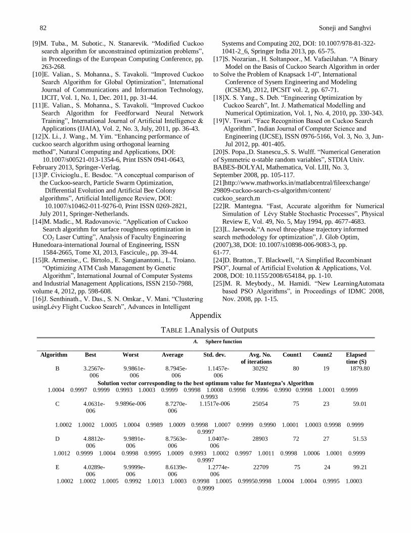
V. Results obtained
With all the modifications B to H of the algorithm described
above, Cuckoo Search algorithm is implemented on above
mentioned benchmark problems A to J. The results obtained
are analyzedin terms of the best and the worst solution, mean
and the standard deviation of the optimum values obtained in
100 runs, the number of optimum values obtain within one
standard deviation interval, and the time of execution for 100
runs.The Count1 and Count2 variables in the table are
showing, out of 100 runs how many optimum values are
obtained within one and two standard deviation interval from
the actual global minimum.The tabulated outputs are shown in the table1 in appendix.
VI. Conclusion
From the outputs obtained, we see that McCulloch algorithm
and simplified version of Mantegna’s algorithm are more
efficient than Mantegna’s algorithm in terms of runtime.
Further,addition of the Local Best term in the simplified
version algorithm gives better results in many problems and comparable results in others with slight increase in the run
time. However, replacing entire vector instead of some of its
components does not reveal any significant improvement in the
result, though it is preferable according to the base of the
algorithm.
VII. Future work
As we have seen that the Cuckoo Search algorithm with simplified version of Mantegna’s algorithm to generate Lévy
flight is improved by adding the Local Best term. This
improved version of CS can also be applied to constrained
optimization problems to check its effect on the performance.
At present, a fraction of the nests are replaced randomly.
Instead, the poorer solutions can be prioritized for removal.
Similarly, the probability of removal can also be varied and its
appropriate value can be sought.
VIII. References
[1]X. -S. Yang., S. Deb.“Cuckoo search via
LévyFlights”,inProceedings of World Congress on Nature & Biologically Inspired Computing (NaBIC 2009), India,
IEEE publications, USA, pp 210-214.
[2]http://cambridge.academia.edu/XinSheYang/Teaching
[3]http://people.unipmn.it/scalas/report1_eng.pdf
[4 H.Soneji., R. C.Sanghvi. “Towards the Improvement of
Cuckoo Search Algorithm”, in Proceedings of World
Congress on Information and Communication
Technologies (WICT), 2012, pp. 878-883.
[5]S. Walten., O. Hassan., K. Morgan., M. R. Brown.
“Modified Cuckoo Search: A new Gradient Free
Optimization Algorithm”, Chaos, Solitons and Fractals, Vol. 44, issue 9, pp. 710-718.
[6]H. Salimi., D. Giveki.,M.Settanshahi., J. Hatami.
“Extended Mixture of MLP Experts by Hybrid of
Conjugate Gradient Method and Modified Cuckoo Search”,
International Journal of Artificial Intelligence &
Applications (IJAIA), Vol. 3, No. 1, Jan. 2012, pp. 1-13.
[7]A. Kaveh., T. Bakshpoori.“Optimum Design of Space
Trusses using Cuckoo Search algorithm with Lévy Flights”,
IJST Transactions of Civil Engineering, Vol. 37, No. C1,
pp. 1-15.
[8]A. R. Yildiz. “Cuckoo Search Algorithm for the
Selection of Optimal Machining Parameters in Milling Operations”, The International Journal of Advanced
Manufacturing Technology, Vol. 64, issue 1-4, pp. 55-61.
82 Soneji and Sanghvi
[9]M. Tuba., M. Subotic., N. Stanarevik. “Modified Cuckoo
search algorithm for unconstrained optimization problems”,
in Proceedings of the European Computing Conference, pp.
263-268. [10]E. Valian., S. Mohanna., S. Tavakoli. “Improved Cuckoo
Search Algorithm for Global Optimization”, International
Journal of Communications and Information Technology,
IJCIT, Vol. 1, No. 1, Dec. 2011, pp. 31-44.
[11]E. Valian., S. Mohanna., S. Tavakoli. “Improved Cuckoo
Search Algorithm for Feedforward Neural Network
Training”, International Journal of Artificial Intelligence &
Applications (IJAIA), Vol. 2, No. 3, July, 2011, pp. 36-43.
[12]X. Li., J. Wang., M. Yim. “Enhancing performance of
cuckoo search algorithm using orthogonal learning
method”, Natural Computing and Applications, DOI:
10.1007/s00521-013-1354-6, Print ISSN 0941-0643, February 2013, Springer-Verlag.
[13]P. Civicioglu., E. Besdoc. “A conceptual comparison of
the Cuckoo-search, Particle Swarm Optimization,
Differential Evolution and Artificial Bee Colony
algorithms”, Artificial Intelligence Review, DOI:
10.1007/s10462-011-9276-0, Print ISSN 0269-2821,
July 2011, Springer-Netherlands.
[14]M. Madic., M. Radovanovic. “Application of Cuckoo
Search algorithm for surface roughness optimization in
CO2 Laser Cutting”, Analysis of Faculty Engineering
Hunedoara-international Journal of Engineering, ISSN 1584-2665, Tome XI, 2013, Fascicule1, pp. 39-44.
[15]R. Armenise., C. Birtolo., E. Sangianantoni., L. Troiano.
“Optimizing ATM Cash Management by Genetic
Algorithm”, International Journal of Computer Systems
and Industrial Management Applications, ISSN 2150-7988,
volume 4, 2012, pp. 598-608.
[16]J. Senthinath., V. Das., S. N. Omkar., V. Mani. “Clustering
usingLévy Flight Cuckoo Search”, Advances in Intelligent
Systems and Computing 202, DOI: 10.1007/978-81-322-
1041-2_6, Springer India 2013, pp. 65-75.
[17]S. Nozarian., H. Soltanpoor., M. VafaeiJahan. “A Binary
Model on the Basis of Cuckoo Search Algorithm in order to Solve the Problem of Knapsack 1-0”, International
Conference of Sysem Engineering and Modeling
(ICSEM), 2012, IPCSIT vol. 2, pp. 67-71.
[18]X. S. Yang., S. Deb. “Engineering Optimization by
Cuckoo Search”, Int. J. Mathematical Modelling and
Numerical Optimization, Vol. 1, No. 4, 2010, pp. 330-343.
[19]V. Tiwari. “Face Recognition Based on Cuckoo Search
Algorithm”, Indian Journal of Computer Science and
Engineering (IJCSE), ISSN 0976-5166, Vol. 3, No. 3, Jun-
Jul 2012, pp. 401-405.
[20]S. Popa.,D. Stanescu.,S. S. Wulff. “Numerical Generation
of Symmetric α-stable random variables”, STDIA Univ. BABES-BOLYAI, Mathematica, Vol. LIII, No. 3,
September 2008, pp. 105-117.
[21]http://www.mathworks.in/matlabcentral/fileexchange/
29809-cuckoo-search-cs-algorithm/content/
cuckoo_search.m
[22]R. Mantegna. “Fast, Accurate algorithm for Numerical
Simulation of Lévy Stable Stochastic Processes”, Physical
Review E, Vol. 49, No. 5, May 1994, pp. 4677-4683.
[23]L. Jaewook.“A novel three-phase trajectory informed
search methodology for optimization”, J. Glob Optim,
(2007),38, DOI: 10.1007/s10898-006-9083-3, pp. 61-77.
[24]D. Bratton., T. Blackwell, “A Simplified Recombinant
PSO”, Journal of Artificial Evolution & Applications, Vol.
2008, DOI: 10.1155/2008/654184, pp. 1-10.
[25]M. R. Meybody., M. Hamidi. “New LearningAutomata
based PSO Algorithms”, in Proceedings of IDMC 2008,
Nov. 2008, pp. 1-15.
Appendix
TABLE 1.Analysis of Outputs
A. Sphere function
Algorithm Best Worst Average Std. dev. Avg. No.
of iterations
Count1 Count2 Elapsed
time (S) B 3.2567e-
006
9.9861e- 006
8.7945e- 006
1.1457e- 006
30292 80 19 1879.80
Solution vector corresponding to the best optimum value for Mantegna’s Algorithm 1.0004 0.9997 0.9999 0.9993 1.0003 0.9999 0.9998 1.0008 0.9998 0.9996 0.9990 0.9998 1.0001 0.9999
0.9993
C 4.0631e-006
9.9896e-006 8.7270e-006
1.1517e-006 25054 75
23 59.01
1.0002 1.0002 1.0005 1.0004 0.9989 1.0009 0.9998 1.0007 0.9999 0.9990 1.0001 1.0003 0.9998 0.9999 0.9997
D 4.8812e-006
9.9891e-006
8.7563e-006
1.0407e-006
28903
72 27 51.53
1.0012 0.9999 1.0004 0.9998 0.9995 1.0009 0.9993 1.0002 0.9997 1.0011 0.9998 1.0006 1.0001 0.9999 0.9997
E 4.0289e-006
9.9999e-006
8.6139e-006
1.2774e-006
22709 75 24 99.21
1.0002 1.0002 1.0005 0.9992 1.0013 1.0003 0.9998 1.0005 0.99950.9998 1.0004 1.0004 0.9995 1.0003
0.9999

Towards the Improvement of Cuckoo Search Algorithm 83
F 5.2293e-006
9.9980e-006
8.8852e-006
1.0104e-006
26732 77 22 99.71
0.9993 1.0000 0.9996 0.9995 0.9999 0.9995 1.0001 0.9992 0.99990.9995 1.0003 0.9991 1.0004 1.0014 1.0004
G 5.6880e-006
5.1930e-005
1.0429e-005
5.1315e-006
54069 94 4 213.36
1.0003 0.9997 0.9996 0.9999 0.9997 0.9997 0.9998 0.9990 0.99981.0000 0.9990 1.0016 1.0009 1.0001 0.9999
H 6.1369e-006
1.3901e-005
9.4048e-006
1.0205e-006
76137 86 11 290.14
1.0003 1.0007 1.0001 0.9992 1.0007 1.0009 0.9994 1.0003 0.99931.0001 0.9985 1.0006 1.0000 0.9998 1.0000
C. Dixon and Price function
B 4.0070e-
006
9.9880e-006
8.7633e-006
1.2430e-006
115242
83 15 7199.48
0.9999 0.7071 0.5946 0.5452 0.5221 0.5107 0.5053 0.5026 0.5013 0.5006 0.5002 0.5001 0.5000 0.4999 0.5000
C 5.2696e-006
9.9917e-006
8.8244e-006
1.0972e-006
71392 73 26 201.72
0.9998 0.7072 0.5947 0.5452 0.5221 0.5109 0.5056 0.5031 0.5015 0.5007 0.5004 0.5001 0.5000 0.5000 0.5000
B. Ackley function
B 6.9467e-006
9.9980e-006
9.3813e-006
6.1186e-007
57215 84 14 3598.08
1.0e-005 * (0.3375 -0.3166 0.2427 -0.0699 0.0433 -0.0203 0.0114 -0.0698 0.2428 0.0054 0.2222 0.0587 -0.1648 -0.1370
-0.0970) C 5.7285e-
006 9.9999e-006
9.2924e-006
7.5327e-007
52180 89 10 169.23
1.0e-005 * (-0.0387 -0.2867 -0.1907 0.0663 -0.0479 -0.1729 -0.0042 0.0668 -0.1799 -0.0315 0.2273 -0.0633 0.1211 0.1667
-0.1226) D 6.8473e-
006 9.9936e-006
9.2404e-006
6.7318e-007
55348 75 23 162.86
1.0e-005 * (-0.0780 -0.0021 0.2249 -0.0665 0.0855 0.0770 -0.0320 -0.3295 -0.1894 -0.1581 -0.0827 0.1628 0.1942 -0.3411
0.0857) E 7.8095e-
006
9.9964e-
006
9.3539e-
006
5.6470e-
007
53849 63 37 309.78
1.0e-005 * (-0.0992 0.1977 0.2953 0.2978 0.0845 0.0079 0.0096 0.2059 0.0914 -0.2830 -0.1501 0.2485 0.3192 -0.1491
0.0202) F 7.8898e-
006 9.9996e-006
9.4820e-006
4.6686e-007
78295 69 30 370.46
1.0e-005 * (0.2066 0.2275 -0.1172 -0.0067 0.2004 0.2766 0.0454 0.1715 -0.0165 -0.4995 0.2424 -0.1002 0.0516 0.0049
-0.0771) G 1.4341e-
005 0.0085 0.0016 0.0017 250050 87 10 1251.39
1.0e-005 * (-0.3341 0.2100 -0.1918 0.0968 -0.0504 0.2523 -0.4797 0.2357 0.0813 -0.4336 0.5124 0.0701 0.1220 0.2327 -
0.9181) H 4.1774e-
005 0.0049 8.1326e-
004 8.7564e-004
250050 87 10 1190.88
1.0e-004 * (0.1513 -0.0048 0.0391 -0.0276 0.1309 0.2200 -0.0659 0.1526 0.00370.1111 0.0178 -0.1662 -0.0196 -0.0047 -
0.0669)

84 Soneji and Sanghvi
D 4.5957e-006
9.9951e-006
8.8336e-006
9.3460e-007
112070 66 33 206.76
0.9989 0.7066 0.5942 0.5451 0.5220 0.5110 0.5053 0.5025 0.5013 0.5007 0.5004 0.5002 0.5001 0.5000 0.5001
E 6.0701e-006
9.9852e-006
9.1036e-006
8.3417e-007
50227 81 18 210.48
1.0009 0.7074 0.5948 0.5452 0.5224 0.5111 0.5057 0.5027 0.50130.5007 0.5002 0.5001 0.5000 0.5000 0.5000
F 6.2179e-006
9.9997e-006
9.0701e-006
9.0783e-007
51948 85 18 180.25
0.9997 0.7069 0.5947 0.5453 0.5220 0.5109 0.5051 0.5024 0.50110.5004 0.5001 0.5000 0.5000 0.4999
0.4999 G 8.0211e-
006 1.4276e-004
1.6982e-005
2.0736e-005
110125 93 5 409.53
1.0008 0.7073 0.5946 0.5453 0.5221 0.5109 0.5054 0.5029 0.5015 0.5006 0.5006 0.5002 0.5001 0.5001 0.5000
H 6.6130e-006
4.0624e-005
1.0180e-005
3.9246e-006
106177 93 5 384.50
1.0010 0.7073 0.5945 0.5451 0.5224 0.5111 0.5056 0.5027 0.5015 0.5007 0.5003 0.5001 0.5001 0.5001
0.5002
D. Griewank function
B 5.7618e-
006
9.9869e-006
8.9680e-006
9.0289e-007
74986 71 28 4644.76
-0.0005 0.0004 -0.0012 0.0022 0.0030 0.0025 0.0030 -0.0035 -0.0007 -0.0044 0.0024 -0.0033 -0.0014 -0.0014 0.0014
C 3.5171e-006
9.9939e-006
8.8725e-006
1.1396e-006
51288 86 12 185.91
-0.0004 -0.0022 -0.0006 -0.0002 -0.0010 -0.0003 -0.0016 -0.0013 -0.0012 -0.0009 -0.0043 -0.0017 0.0043 -0.0002 -0.0007
D 4.5841e-006
9.9939e-006
9.0155e-006
9.3623e-007
80841
81 18 197.59
0.05 0.0009 0.0000 0.0024 0.0001 0.0011 -0.0006 -0.0006 0.0015 -0.0031 0.0059 0.0046 -0.0000 0.0029 0.0011
E 5.0555e-006
9.9961e-006
8.5652e-006
1.0888e-006
34027 72 27 187.47
0.0019 -0.0001 -0.0005 0.0005 0.0022 0.0031 -0.0013 -0.0032 -0.0019 -0.0007 0.0014 -0.0001 0.0036 0.0011 -
0.0028 F 5.1481e-
006 9.9938e-006
8.8811e-006
1.0742e-006
33657 81 16 155.46
-0.0005 -0.0002 0.0004 0.0031 0.0018 0.0054 -0.0000 -0.0013 0.00220.0002 0.0022 -0.0025 0.0007 0.0013 0.0002
G 4.9378e-006
9.9996e-006
9.2825e-006
8.4246e-007
33595 88 10 162.55
0.0007 -0.0002 -0.0030 0.0040 -0.0001 0.0015 -0.0007 -0.0023 0.00100.0000 0.0014 -0.0022 -0.0008 0.0001
0.0021 H 5.5236e-
006 9.9919e-006
8.9231e-006
9.7572e-007
79051 78 20 369.77
0.0011 -0.0001 -0.0008 0.0005 0.0007 0.0023 0.0006 -0.0010 0.0035-0.0060 -0.0008 -0.0038 -0.0013 -0.0015 -0.0053
E. Step function
B 5.7994e-006
9.9997e-006
9.3504e-006
7.1027e-007
64890 87 11 49324.45
-0.5000 -0.5000 -0.5000 -0.5000 -0.5000 -0.5000 -0.5000 -0.5000 -0.5000 -0.5000 -0.5000 -0.5000 -0.5000 -0.5000 -0.5000

Towards the Improvement of Cuckoo Search Algorithm 85
C 7.0603e-006
9.9921e-006
9.3225e-006
6.6777e-007
53039 83 15 119.74
-0.5000 -0.5000 -0.5000 -0.5000 -0.5000 -0.5000 -0.5000 -0.5000 -0.5000 -0.5000 -0.5000 -0.5000 -0.5000 -0.5000 -0.5000
D 6.0982e-006
9.9998e-006
9.3788e-006
6.3441e-007
63368
90 9 86.10
-0.5000 -0.5000 -0.5000 -0.5000 -0.5000 -0.5000 -0.5000 -0.5000 -0.5000 -0.5000 -0.5000 -0.5000 -0.5000 -0.5000 -0.5000
E 6.1740e-006
9.9913e-006
9.2191e-006
7.0416e-007
56561 80 18 189.73
-0.5000 -0.5000 -0.5000 -0.5000 -0.5000 -0.5000 -0.5000 -0.5000 -0.5000 -0.5000 -0.5000 -0.5000 -0.5000 -0.5000 -0.5000
F 6.5182e-006
9.9978e-006
9.3144e-006
7.4204e-007
67043 83 16 230.05
-0.5000 -0.5000 -0.5000 -0.5000 -0.5000 -0.5000 -0.5000 -0.5000 -0.5000 -0.5000 -0.5000 -0.5000 -0.5000 -0.5000 -0.5000
G 3.5900e-004
0.0237 0.0055
0.0040 250050 75 24 864.14
-0.5000 -0.5000 -0.5001 -0.4999 -0.5000 -0.4999 -0.5000 -0.5000 -0.5000-0.4999 -0.5000 -0.5000 -0.5000 -0.5000 -0.5000
H 3.6564e-004
0.0177 0.0044 0.0030 250050 81 17 892.24
-0.5000 -0.4998 -0.5000 -0.5000 -0.5000 -0.5000 -0.5000 -0.5000 -0.5000 -0.5000 -0.5000 -0.5000 -0.4998 -0.5000 -0.5000
F. Levy function
B 5.2459e-
006
9.9702e-
006
8.6432e-
006
1.1694e-
006
49029
67 33 6137.60
0.9999 1.0012 0.9993 1.0001 1.0006 0.9988 0.9992 0.9994 0.9994 0.9992 1.0000 0.9998 0.9986 1.0004 0.9955
C 4.2144e-006
9.9917e-006
8.8422e-006
1.2086e-006
52165
85 13 338.76
1.0000 0.9993 0.9988 0.9991 0.9996 1.0005 0.9990 0.9992 1.0005 0.9995 1.0002 0.9988 1.0007 0.9996
1.0025
D 6.2420e-006
9.9940e-006
8.8758e-006
9.2807e-007
40731 68 32 228.21
0.9992 0.9996 1.0018 1.0005 0.9985 0.9991 0.9998 0.9996 0.9988 0.9994 0.9994 1.0013 0.9996 0.9998 0.9994
E 3.6972e-006
9.9763e-006
8.9246e-006
1.1450e-006
49005 86 12 345.55
0.9997 1.0001 1.0005 1.0001 1.0003 0.9998 1.0013 0.9988 1.00041.0008 0.9991 1.0006 1.0000 0.9992 1.0028
F 5.7284e-006
9.9887e-006
8.7916e-006
1.0038e-006
51325 69 30 368.60
0.9994 1.0007 0.9993 1.0005 0.9994 1.0004 1.0002 0.9975 1.00041.0006 1.0007 1.0010 1.0008 0.9999 0.9991
G 7.2409e-006
1.3956e-004
1.7626e-005
2.0639e-005
125180 91 5 2142.80
1.0004 1.0004 1.0009 1.0014 0.9984 0.9996 0.9999 0.9990 1.0002 0.9984 1.0003 1.0010 1.0000 0.9994 1.0053
H 7.0236e-006
0.0010 2.1247e-005
1.0299e-004
168845 99 0 1291.43
0.9988 0.9993 0.9989 1.0003 0.9987 1.0011 0.9995 0.9997 1.00061.0002 1.0001 1.0000 1.0023 0.9997 0.9991
G. Generalized Schwfel 2.6 function
B 1.9095e-
004
1.9100e-
004
1.9099e-
004
1.1584e-
008
47138
75 25 2830.24

86 Soneji and Sanghvi
420.9688 420.9689 420.9688 420.9685 420.9690 420.9690 420.9688 420.9687 420.9690 420.9686 420.9686 420.9687 420.9686 420.9688 420.9689
C 1.9095e-004
1.9100e-004
1.9099e-004
1.1858e-008
39452
75 25 130.09
420.9686 420.9689 420.9686 420.9689 420.9687 420.9689 420.9687 420.9689 420.9687 420.9686 420.9688 420.9688 420.9686 420.9685 420.9684
D 1.9095e-004
1.9100e-004
1.9099e-004
9.8004e-009
47343 70 29 117.09
420.9686 420.9686 420.9687 420.9686 420.9684 420.9686 420.9689 420.9688 420.9688 420.9687 420.9688 420.9687
420.9690 420.9689 420.9688 E 1.9095e-
004 1.9099e-004
1.9098e-004
7.9203e-009
40190 82 17 162.97
420.9687 420.9687 420.9688 420.9690 420.9689 420.9690 420.9687 420.9688 420.9688420.9685 420.9688 420.9687 420.9686 420.9687 420.9689
F 1.9095e-004
1.9099e-004
1.9098e-004
8.5980e-009
49122 88 9 202.44
420.9687 420.9688 420.9686 420.9685 420.9689 420.9688 420.9687 420.9688 420.9689420.9688 420.9687 420.9687
420.9685 420.9688 420.9688 G 1.9098e-
004 0.0031 3.4766e-
004 3.6788e-004
242458 94 4 1059.23
420.9688 420.9690 420.9688 420.9688 420.9688 420.9690 420.9689 420.9690 420.9690420.9687 420.9690 420.9686 420.9692 420.9687 420.9688
H 1.9098e-004
5.4799e-004
2.3815e-004
7.7540e-005
245545 87 10 1048.99
420.9690 420.9687 420.9687 420.9687 420.9687 420.9688 420.9684 420.9692 420.9687 420.9684 420.9688 420.9689
420.9686 420.9686 420.9689
H. Generalized Rozenbrock function
B 5.9126e-
006
9.9910e-006
9.0904e-006
8.9282e-007
180592
82 17 10935.36
1.0000 1.0000 1.0000 0.9999 0.9999 0.9999 1.0000 1.0000 1.0000 0.9999 0.9999 0.9998 0.9997 0.9994 0.9988
C 5.2451e-006
9.9989e-006
8.7796e-006
1.2255e-006
153918
80 20 416.28
1.0000 1.0001 1.0001 1.0001 1.0001 1.0000 1.0000 1.0000 1.0000 1.0000 1.0000 0.9999 0.9998 0.9996 0.9992
D 3.5767e-006
9.9861e-006
8.9595e-006
1.0825e-006
178861
87 11 342.38
1.0000 1.0000 1.0000 1.0000 1.0000 1.0000 1.0000 1.0000 1.0000 1.0000 0.9999 0.9999 0.9997 0.9993 0.9987
E 6.4442e-006
9.9679e-006
9.1012e-006
8.6809e-007
178901 85 14 604.98
1.0000 1.0000 1.0000 1.0000 1.0000 1.0000 1.0001 1.0001 1.00001.0000 1.0001 1.0001 1.0002 1.0004 1.0009
F 3.3758e-006
9.9981e-006
8.9790e-006
1.3726e-006
2786167 88 9 9695.60
1.0000 1.0000 1.0000 1.0000 1.0000 1.0000 1.0000 1.0000 1.00011.0001 1.0001 1.0001 1.0002 1.0004 1.0010
G 0.0049 4.2062 0.2952 0.5756 250050 96 2 915.23 0.9997 0.9996 0.9980 0.9990 1.0010 1.0004 1.0003 1.0006 1.00181.0007 0.9985 0.9959 0.9912 0.9823
0.9629 H 0.0018 6.6209 0.6577 0.9572 250050 92 5 898.87
0.9992 1.0000 1.0010 0.9999 1.0008 1.0007 0.9996 0.9999 1.00011.0006 1.0007 1.0012 1.0029 1.0044 1.0080
I. Rastrigin function
B 5.1106e-
006
9.9937e-006
8.8557e-006
1.1609e-006
148996
85 14 17878.04
1.0e-004 * (0.0172 -0.1457 -0.0348 -0.0636 0.7672 0.5330 -0.2948 -0.2397 -0.2673 -0.1595 -0.6657 0.6431 0.7142 0.2578
-0.0454) C 5.7378e- 9.9983e- 8.9440e- 1.0180e- 117280 79 19 335.70

Towards the Improvement of Cuckoo Search Algorithm 87
006
006
006
006
1.0e-004 * (-0.2367 0.6540 -0.5494 -0.3404 -0.6498 -0.4619 0.1200 -0.4927 -0.0967 -0.3726 0.1325 -0.3121 -0.4535 0.1428
0.7801)
D 5.1870e-006
9.9959e-006
8.8865e-006
1.0213e-006
150460
79 20 308.76
1.0e-004 * (0.5935 0.6347 0.2006 0.1777 -0.7579 -0.2038 -0.2997 -0.4182 0.0807 0.3540 -0.0561 0.5301 -0.0770 0.6941 -
0.0572) E 4.6449e-
006
9.9969e-
006
8.9237e-
006
9.3483e-
007
111777 73 25 388.30
1.0e-004 * (-0.4289 0.3301 0.0170 -0.5071 -0.2502 0.4892 -0.0266 -0.0260 0.25200.9068 0.2732 0.1134 -0.4025 -0.2850
0.5206) F 5.3737e-
006 9.9841e-006
8.7024e-006
1.1478e-006
76599 71 29 273.38
1.0e-004 * (0.6769 -0.6097 0.0239 -0.5833 -0.1260 0.1887 0.4944 0.1008 -0.38200.4067 -0.5938 0.1867 0.1583 0.6833
0.2029) G 7.9957e-
006 2.7199 0.1361 0.5957 209400 95 0 798.18
1.0e-003 * (-0.0002 0.0348 -0.0592 -0.0554 0.0334 0.0338 -0.0575 0.0279 -0.0530-0.0350 0.0419 0.1259 -0.0298 0.0550
0.0249) H 8.4836e-
006 5.5275 1.3070 1.6926 249068 91 9 926.86
1.0e-003 *
( -0.0412 0.0288 -0.0448 -0.1092 0.1265 0.0195 -0.0147 -0.0286 -0.0054 -0.0458 -0.0712 0.0281 0.0224 0.0194 0.0006 )
J. Weierstrass function
B 5.6438e-
006
9.9953e-006
9.0794e-006
9.1828e-007
152255
83 15 13062.56
1.0e-010* ( -0.3072 0.1276 0.7386 0.3193 0.4202 0.1431 -0.1365 -0.1628 0.0228 -0.0438 -0.0686 -0.3037 -0.2694 0.9639
-0.4146)
C 5.0205e-006
9.9779e-006
8.8138e-006
1.1420e-006
176001
84 15 5320.60
1.0e-009 * (-0.0442 -0.0088 0.1289 -0.0145 -0.0030 0.0144 0.0120 -0.0303 0.0051 -0.0424 0.0067 -0.0068 -0.0249 -0.0119
0.0372) D 6.0728e-
006
9.9969e-006
9.1135e-006
8.1877e-007
152575
72 26 4257.29
1.0e-010 * ( -0.4487 -0.3217 -0.2167 -0.1818 0.1428 0.0274 -0.1441 0.1908 0.3232 -0.3613 0.6083 0.8060 0.7243 0.3006
0.0619) E 4.5747e-
006 9.9979e-006
8.8024e-006
1.1522e-006
147530 81 16 4566.94
1.0e-010 * ( 0.6775 -0.0590 -0.1896 -0.0588 0.1378 -0.3148 0.4213 -0.1647 -0.1570 -0.5015 0.7391 -0.1638 -0.1933 0.0000 -
0.1660) F 5.5391e-
006 9.9964e-006
9.1979e-006
9.0840e-007
165474 87 11 5090.04
1.0e-009 * ( 0.0110 0.0271 0.0178 -0.0601 -0.0174 -0.0079 -0.1396 0.0202 -0.03680.0235 0.0043 -0.0246 0.0053 -0.0267 -
0.0002)
G 0.0827 1.3395 0.3113 0.2484 250050 89 7 8400.94 1.0e-003 *
(0.0006 -0.0189 0.0000 -0.0000 0.0006 -0.0030 -0.0000 0.0050 -0.1524 0.0000 -0.0339 -0.0002 0.4575 -0.0000 -0.0621)
H 0.0697 1.0990 0.2130 0.1132 250050 92 7 7697.71

88 Soneji and Sanghvi
1.0e-003 * (0.0081 -0.0009 -0.0017 -0.0004 0.1132 0.0001 -0.0022 -0.1394 0.0150-0.0342 0.0357 0.0002 0.0018 -0.0003
0.0007)