Proceedings of the Second APSIPA Annual Summit and Conference, pages 609–618,Biopolis, Singapore, 14-17 December 2010.

Towards the Next Video Standard: High EfficiencyVideo Coding

Hsueh-Ming Hang1, Wen-Hsiao Peng2, Chia-Hsin Chan3 and Chun-Chi Chen41Department of Electronics Engineering, National Chiao Tung University

E-mail:hmhang@mail.nctu.edu.tw2−4Department of Computer Science, National Chiao Tung University

E-mail:2pawn@mail.si2lab.org, 3terry0201.cs98g@nctu.edu.tw, 4cheerchen.cs98g@g2.nctu.edu.tw

Abstract—After the profound success of defining H.264/AVCvideo coding standard in 2002, ITU-T Video Coding ExpertsGroup (VCEG) started a Next-generation Video Coding (NGVC)project. The original target is to achieve 50% bit rate re-duction at about the same video quality. In the past a fewyears, researchers have been very actively searching for new orimproved technologies that can achieve this goal. After severalyears’ struggle, in January 2010, the ISO/IEC Motion PictureExpert Group (MPEG) and VCEG jointly issued a call-for-proposal for the “High Efficiency Video Coding (HEVC)”. Atthe April VCEG/MPEG meeting, 27 proposals were evaluatedand the results seem to be promising. Consequently, a “new”video standard may be defined in two years. We will present alimited and maybe biased view on this subject.

I. INTRODUCTION

The success of recent multimedia systems such as digital TVand digital camera are often contributed to the standardizationof video/audio compression algorithms and the wide spread ofpersonal computer, Internets, and wireless technologies. Theadvance of digital video compression in the last three decadeshas produced fruitful results in the past 10 years. Severalinternational image and video coding scenarios have been stan-dardized, for example, ITU H.261/H.263 for video telephony,ISO/IEC JPEG for still images, and ISO/IEC MPEG-1 andMPEG-2 for video CD and digital TV [1][2][3]. After theobject- oriented video coding standard, MPEG-4 part 2, wasproduced, the most significant addition to the video codingstandards was H.264/MPEG-4 Advanced Video Coding (AVC)standard finalized in 2003 [3][4]. Since then, many peoplehave tried to design a video coding algorithm more efficientthan AVC. In February 2010, 27 proposals submitted to theITU/ISO joint committee competing for the next generationvideo standard. The proposal evaluation results in the Aprilstandard meeting indicated that a better coding scheme ispossible and thus the High Efficiency Video Coding (HEVC)work item was launched.In the rest of this paper, we will first cover the basic

image/video techniques adopted by the international ITU/ISOstandards before 2010 in Section II. Then, we will describethe progress of the HEVC standard activities in Section III.In Section IV, we show some comparisons with respect tothe coding efficiency and complexity between the currentlyreleased HEVC software and the AVC JM software. The main

body of this article, Section V, is dedicated to a summary ofnew tools that may be included in HEVC. At the end, we adda few words on the projection of this standard and the videocoding research trends.

II. FROM JPEG TO AVC

Historically, the modern image/video coding standard ac-tivity started in 1984 and the target was for video telephony.The output of this activity is CCITT (ITU) H.261. However,in logical order, the simple still image standard (JPEG) will befirst described below and then followed by the more complexmoving image standards.The International Standards Organization (ISO) Joint Pho-

tographic Experts Troup (JPEG) spent several years in de-veloping an algorithm for compressing still images. In 1987,10 proposals were evaluated and the adaptive DCT schemestood out. Although major technical points were agreed inabout 1989, the JPEG standard (ISO 10918-1) was formallyfinalized in 1992 [1][2]. The core of this algorithm is the so-call transform coding technique, which converts the digitizedpicture samples (pixels or pels) into transform coefficients.The correlation of highly redundant pixels in spatial domainis largely removed by DCT. In addition, for most naturalpictures, DCT packs the originally scattered power in thespatial domain into a few low frequency components in thetransform domain. Transform coefficients are then quantizedto reduce the transmission bit rate.To further reduce the average transmission bit rate, the

frequently occurred events (quantized coefficient patterns) areassigned short codes, and the seldom occurred events, longcodes. This procedure is the so-called Variable Word-LengthCoding (VLC), a modified version of the well-known Huffmancode. For typical natural (color) pictures, JPEG algorithmoffers a compression ratio of 10 to 20 (or 1 to 2 bits perpixel) with good image quality.In 1984, CCITT (International Telegraph and Telephone

Consultative Committee) started a standard for sending video-phone (and videoconference) pictures through ISDN. A set ofsuch standards was finalized in 1990, also known as the px64kstandards [1][2]. In addition to the DCT coding technique, theblock motion compensation technique is adopted by CCITT

609

10-0106090618©2010 APSIPA. All rights reserved.

2D (8x8)DCT

Framememory

Bitstream

Inputframe

Loopfilter

MotionEstimator

Q-1

2D (8x8)IDCT

VLC

VLC

Motion vectors

Previous reconstructed frame

inter

intra1

0

Σ0inter

intra1

++

Σ+

Mul

tiple

x

& B

uffe

r

Q

Coding Control

Fig. 1. The H.261 RM8encoder structure.

H.261 [1][2][3]. Fig. 1 shows a typical H.261 encoder (Ref-erence Model 8) [5]. In fact, the same basic coding structureis inherited by all the video standards mentioned in SectionI. More precisely, the standards specify only the decoder;however, reference encoders are provided in the standarddocuments and they are pretty much viewed as the typicalencoders in implementation.To save transmission bandwidth, only the parts of a pic-

ture that change from frame to frame are sent. The motionestimation technique calculates the displacement vector of aMacroblock (16 pels by 16 lines) that moves from the previ-ous frame to the current frame. Then, the prediction errors,differences between the current frame pixels and the displaced(or motion-compensated) previous frame pixels, are coded andtransmitted along with the corresponding displacement vector.In H.261, either the original image block or the predictionerror block is DCT-transformed (DCT), quantized (Q), andthen VLC-coded.To further increase the compression efficiency, the

ISO Moving Picture Experts Group (MPEG) adopted therather complicated motion-compensated interpolation tech-nique [1][2][3]. This is the main difference between theH.261 algorithm and the MPEG algorithm. Either the previousframe or the future frame (in camera acquisition) or bothof them can be used in MPEG to produce the prediction(interpolation) errors. Thus, the so-called future frame has tobe coded and transmitted before the current frame. Therefore,the transmission order of pictures is different from the ordertaken at camera. At about 4 Mb/s, MPEG-2 can produce verygood quality pictures at regular TV picture resolutions. It thusbecame the video standards of DVD and digital TV. The ISOMPEG group was established in 1988 and the MPEG-1 video(ISO 11172 part 2) and MPEG-2 video (ISO 13818 part 2)were finalized in 1992 and 1994, respectively.In 1993, the ITU-T Video Coding Experts Group (VCEG)

started new work items. A Near-Term project was targetingat improving H.261 and a Long-Term project was develop-ing a more efficient coding scheme that may be differentfrom H.261. The Near-Term project produced H.263 in 1995

and the Long-Term project (H.26L) led to the well-knownH.264/MPEG-4 AVC standard [3][4]. The core technologyadopted by AVC is the old hybrid transform coding structureshown in Fig. 1. However, every function block in Fig. 1was fine-tuned to produce significantly better overall codingresults. It has been reported by several studies that for typicalTV pictures, AVC reduces the bit rate of MPEG-2 by about50% at the same visual quality [6][7]. Continuing along thesmaller 8×8 block motion compensation trend in MPEG-2and H.263, AVC allows 16×8 (8×16), 8×4 (4×8), and 4×4partitions for motion prediction [4].

III. JOINT COLLABORATIVE TEAM ACTIVITIES

A call-for-proposal was issued in 1998 by ITU VCEG. Thegoal is a low-bit rate, low delay video codec, which was calledH.26L then. After a few years of development, VCEG andthe MPEG video group formed the Joint Video Team (JVT)in 2001. The final AVC standard was produced by JVT in2003. Since then, VCEG launched an exploration activity onthe Next-Generation Video Coding (NGVC) project. Its targetwas to further reduce the video compression bit rate by 50%over AVC. However, the high compression efficiency of AVCis hard to beat. Many new algorithms were proposed to furtherimprove the coding efficiency, but few could show significantlybetter performance. As time goes by, the AVC tools werefurther refined and people noticed some modifications wereable to produce a certain amount of improvement. Thesemodifications were collected and formed a piece of softwarecalled Key Technical Areas (KTA) [8] since 2005.The KTA scheme is more or less an expansion of AVC but

with careful tuning on all the components. In June 2009, theMPEG video group held a call-for-evidence activity. Severalschemes based on KTA were submitted. It showed that a 30%or so coding gain over AVC was possible on higher resolutionvideos. Thus, ITU VCEG and MPEG worked together againand formed the so-called Joint Collaborative Team on VideoCoding (JCT-VC) in January 2010. A joint Call-for-Proposal(CfP) for High Performance Video Coding (HVC) was issued.All the proponents had to submit their test material beforeFebruary 22, 2010.The main goals of HVC stated in the requirement docu-

ment are (a) coding performance on high resolution pictures,(b) picture size up to 8K×4K, (c) low delay, and (d) lowcomplexity [9]. Although the MPEG requirement documentdoes not specify the compression efficiency improvement, theITU NGVC requirements do hope that there is a 50% bit ratereduction over AVC [10].The joint CfP for HVC is a quite lengthy document [11].

There are 5 Classes of test sequences: (A) 2560×1600 croppedfrom 4K×2K, 2 sequences; (B) 1920×1080p, 24/50-60 fps, 5sequences; (C) 832×480 WVGA, 4 sequences; (D) 416×240WQVGA, 4 sequences; and (E) 1280×720p, 50-60 fps, 3sequences. A number of test points (conditions) are specified.They belong to two constraint categories. Constraint 1 (CS1)is the Random Access setting for Classes A to D; a delayof 8-picture GOP is allowed. Constraint 2 (CS2) is the Low

610

Fig. 2. Overall average MOS results over all Classes for CS2.

Delay setting for Classes B to E, and no picture re-ordering isallowed. For comparison purpose, three Anchors are defined.They are the same AVC coding schemes with different codingprofiles and parameters. The Alpha Anchor meets CS1 condi-tions, and the Beta and Gamma Anchors meet CS2. Since thecoding results of three Anchors were published before the CfPdue date, all submissions are at least as good as the Anchors.

In total, 27 proposals, which is historical high in MPEG CfPcompetitions, were submitted to JCT-VC in February and thesubjective image quality evaluation was done in March. Theevaluation results were discussed in the April JCT-VC meetingat Dresden, Germany. A number of key players in video codingcommunity participated in this competition. Objectively, thetop-performers achieve 40% BD-rate [12] savings on CS1,40% and 55% on CS2. Also, the detailed description of thesubjective evaluation results are given in [13]. Limited byspace, we copy only one summary plot that shows the codingperformance of all proposals including the Anchors. Fig. 2is the average Mean Opinion Scores (MOS) of 27 proposalsplus the Beta and Gamma Anchors for CS2. The Anchors arethe lowest two on the right margin in both figures. It is clearthat the best proposal is quite a bit better than the Anchors.Similar observations can be found for CS1 coding conditions.Although there is no single proposal did the best for allpictures at all rate points (5 rate points for each sequence), thegood schemes together are quite promising. Therefore, it wasstated in the conclusion of [13] that “for a considerable numberof test points, the subjective quality of the proposal encodingwas as good, for the best performing proposals, as the qualityof the anchors with roughly double the bit rate”. However,when we examine the techniques used by all these proposals,“all proposed algorithms were based on the traditional hybridcoding approach combining motion-compensated predictionbetween video frames with intra-picture prediction, closed-loop operation with in-loop filtering, 2D transformation ofthe spatial residual signals, and advanced adaptive entropycoding” [13]. These schemes are roughly the expansion andrefinements of KTA, which is an extension of AVC. Becauseof the encouraging testing results, JCT-VC is constructing aTest Model under Consideration (TMuC) [14] described in thenext section. If the standardization process runs smoothly, wemay have a new video standard in two years.

TABLE ITHE DIFFERENCE OF TOOL SELECTIONS BETWEEN HIGH EFFICIENCY AND

LOW COMPLEXITY SETTINGS.

Features High Efficiency Low ComplexityTransform partitioning Quad-tree TU [16]Motion Sharing Merge Mode [16]Intra Pre-filtering Adaptive Intra Smoothing [16]Intra Prediction Combined [17], angular [18], planar [18]Directional Transform MDDT [19], Rotational Transform [20]Deblocking Filter [18] ONAdaptive Scanning [19] ONEntropy Coding PIPE [16] CAVLC [18]Interpolation Filter 12-tap SIFO [19] Directional Filter [18]Adaptive MV Res. [19] ON OFFAdaptive Loop Filter [19] ON OFFIBDI [21] 4 bits 0 bit

IV. CURRENT TMUC STATUS

A. TMuC

After the CfP competition in the 1st JCT-VC meeting,TMuC is constructed mainly from the best performer’s code-base and the other top-performing HEVC proposals. The toolscurrently included in TMuC may not get into the JCT-VCcommittee’s final Test Model1. Rather, these tools are merelya preliminary selection and require further evaluation andjustification. In the current status, TMuC serves as a goodstarting point at the very beginning of the collaborative phase,and aims at creating a minimum set of well-tested tools toestablish the "Test Model 1.0".JCT-VC committee specifies 6 reference configurations [15]

for Tool Experiments (TE). Five test scenarios are classifiedinto two groups: (a) High Efficiency (HE) and Low Complexity(LC) settings; and (b) Intra Only, Random Access, and LowDelay settings. Six test conditions (or configurations) areformed by picking up one from the first group and oneform the second group. Under these testing conditions, theexperimental results are expected to provide insights of thecontribution of a specific tool to the overall performance ofTMuC. It also helps us in defining the profiles for differentapplications. Table I shows the tool selections in group (a)in TMuC. The HE setting aims at achieving the high codingefficiency close to that of the best performing proposal, whilethe LC setting intends to lower the complexity close to thatof the lowest complexity proposals with a relatively highcoding efficiency. Different settings in (b) use different codingstructures to achieve the target functions or features. RandomAccess and Low Delay settings are the same as that in CfP, andthe Intra Only scenario contains only the intra-coded frames.Some experimental results using the reference configurationsare in Section IV-B and IV-C, to compare TMuC with JM.

B. Compression Performance of TMuC

To see the current TMuC coding performance, experimentsare conducted on TMuC 0.7 [14] in comparison with the CfPAnchors generated by JM 16.2 [22]. We exclude Intra Onlysettings and apply the other 4 configurations in [15]. The

1Test Model is a common test platform such as the JM software for AVC.

611

TABLE IISUMMARY OF TMUC BD-RATE SAVINGS.

Random Access Low Delayvs Alpha HE vs vs Gamma HE vs

Class Seq HE LC LC HE LC LCClass A S01 38.9 21.8 21.6 N/A N/A N/A2560×1600 S02 24.9 4.8 19.5 N/A N/A N/AClass B S03 45.6 29.5 22.9 56.7 45.6 19.71920×1080 S04 32.3 14.3 21.1 40.8 25.4 20.5

S05 40.1 21.0 23.5 48.2 32.6 20.3S06 45.3 27.5 23.9 51.2 36.2 23.3S07 48.8 19.9 33.2 63.6 38.9 34.6

Class C S08 39.5 24.0 20.4 44.7 28.2 21.3832×480 S09 37.4 20.5 21.4 41.5 24.8 21.9

S10 36.7 13.1 30.0 38.6 17.9 29.2S11 34.0 21.9 15.7 35.1 24.1 14.2

Class D S12 29.3 16.7 15.3 32.6 22.3 13.4416×240 S13 49.4 3.8 47.2 58.1 10.1 48.3

S14 30.4 10.6 22.5 32.1 13.3 22.3S15 26.4 12.6 15.8 24.8 12.4 14.3

Class E S16 N/A N/A N/A 53.8 26.8 32.61280×720 S17 N/A N/A N/A 50.9 16.3 36.6

S18 N/A N/A N/A 54.3 28.0 32.2Total Avg. 37.2 17.5 23.6 45.4 25.2 25.3

results are compared with CfP Alpha and Gamma Anchors. Toprovide a fair comparison, Gamma Anchor is selected insteadof Beta since its coding structure (IPPP) is similar to that ofTMuC Low Delay setting (IBBB).Table II summarizes the BD-rate [12] savings for each

test sequence. TMuC achieves 4%∼64% BD-rate savingsas compared with JM. Roughly speaking, the coding gainincreases with the increasing sequence resolution. However,the coding gain of Class A is lower than that of Class B. Thereason may be the immature camera acquisition technology,which results in high capturing noise at ultra-high definition(UHD) resolutions. This is also the reason why Class A did notgo under subjective tests in CfP evaluation. Interestingly, somesequences in Class D have significant coding gains, whichindicate that the coding tools in TMuC also work well on lowresolution sequences.Comparing the HE and LC settings, the HE setting always

outperforms the LC setting for more than 13%. Particularly,for S13, the LC setting has a significant loss in coding gainin comparison with the HE setting. The coding gain drops ofthe Low Delay case ranges from 58% to 10%. This anomalymay due to disabling some coding tools at the LC setting.Fig. 3 shows the coded pictures using the CfP Anchors and

TMuC. Apparently, in addition to the objective PSNR metric,the subjective image quality has been significantly improved.Since TMuC is in its early stage of development, furtherimprovement is expected in later versions.

C. Encoding/Decoding Complexity of TMuC

Since a formal complexity measuring index for the TMuCsoftware is not established yet, we try to roughly measure thecomplexity using the encoding and the decoding executiontime. Note that the variations in execution platform andcompiler optimization may lead to different results.

(a)

(b)

Fig. 3. Subjective comparisons between CfP Anchor (left), TMuC LC (mid-dle), and HE (right) settings at the lowest rate points of (a) the Random Accesssetting (S07 frame #290), and (b) the Low Delay setting (S06 frame #7).

It is observed that the LC setting indeed shows lowercomplexity in both encoding and decoding time. The HEsetting is, on average, about 3 times slower than the LC settingfor encoding, and 1.5 times slower for decoding. As comparedwith JM in decoding time, TMuC is apparently slower for atleast 2.8 times. Especially, for Class D, TMuC is even muchslower than JM for more than 11 times; however, TMuC stillcan run on a typical PC at 10∼15 fps. However, for large-sizepictures, the decoder produces only 2∼3 fps for Class A andB. To sum up, TMuC also has plenty of room for improvementin computational complexity.

V. CURRENT HEVC TOOLS SUMMARY

In the conventional video coding standards up to now, mostcoding tools use fixed parameters or operations to simplifyimplementation. For example, half-pel interpolation is doneby a fixed 6-tap FIR filter in AVC. However, the UHD videocontents show strong signal variations and thus the currentfixed-parameter coding tools are unable to produce the bestpossible results. Therefore, the content- and context-adaptivetools emerge in the next-generation video coding design. Theychange coding parameters on the fly to optimize the codingperformance for time and spatial varying signals. Because theadaptive processes usually involve multi-pass encoding opti-mization, a massively parallel processing architecture becomesincreasingly important for real-time implementation.Based on the above observations, most HEVC proposals

use highly adaptive and complex coding tools. Also, theparallel processing features are emphasized. As describedearlier, the top-performers outperform the Anchors quite a bitboth objectively and subjectively. How could these proposalswith the same basic structure as AVC achieve such a highperformance? We summarize the new tool features in TableIII. Details are given in the following sections.

A. Coding, Prediction and Transform Partitioning

Block-based hybrid video coding structure is the core ofall the current video coding standards. Its basic unit for

612

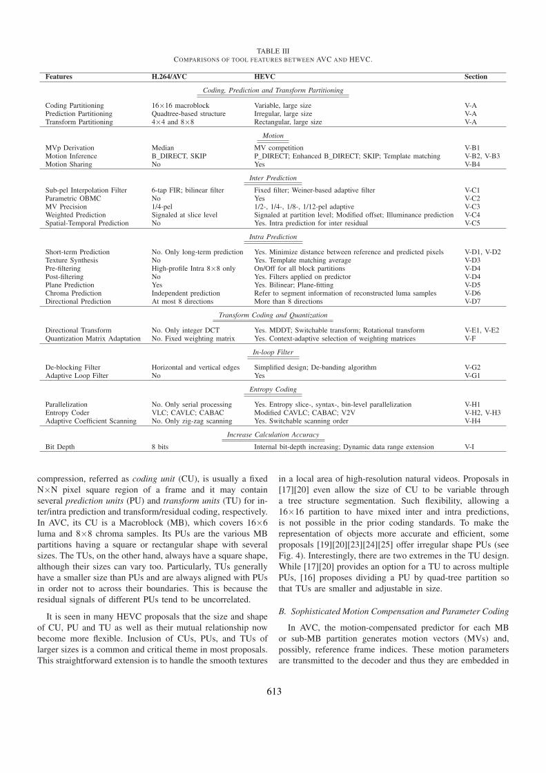
TABLE IIICOMPARISONS OF TOOL FEATURES BETWEEN AVC AND HEVC.

Features H.264/AVC HEVC Section

Coding, Prediction and Transform Partitioning

Coding Partitioning 16×16 macroblock Variable, large size V-APrediction Partitioning Quadtree-based structure Irregular, large size V-ATransform Partitioning 4×4 and 8×8 Rectangular, large size V-A

Motion

MVp Derivation Median MV competition V-B1Motion Inference B_DIRECT, SKIP P_DIRECT; Enhanced B_DIRECT; SKIP; Template matching V-B2, V-B3Motion Sharing No Yes V-B4

Inter Prediction

Sub-pel Interpolation Filter 6-tap FIR; bilinear filter Fixed filter; Weiner-based adaptive filter V-C1Parametric OBMC No Yes V-C2MV Precision 1/4-pel 1/2-, 1/4-, 1/8-, 1/12-pel adaptive V-C3Weighted Prediction Signaled at slice level Signaled at partition level; Modified offset; Illuminance prediction V-C4Spatial-Temporal Prediction No Yes. Intra prediction for inter residual V-C5

Intra Prediction

Short-term Prediction No. Only long-term prediction Yes. Minimize distance between reference and predicted pixels V-D1, V-D2Texture Synthesis No Yes. Template matching average V-D3Pre-filtering High-profile Intra 8×8 only On/Off for all block partitions V-D4Post-filtering No Yes. Filters applied on predictor V-D4Plane Prediction Yes Yes. Bilinear; Plane-fitting V-D5Chroma Prediction Independent prediction Refer to segment information of reconstructed luma samples V-D6Directional Prediction At most 8 directions More than 8 directions V-D7

Transform Coding and Quantization

Directional Transform No. Only integer DCT Yes. MDDT; Switchable transform; Rotational transform V-E1, V-E2Quantization Matrix Adaptation No. Fixed weighting matrix Yes. Context-adaptive selection of weighting matrices V-F

In-loop Filter

De-blocking Filter Horizontal and vertical edges Simplified design; De-banding algorithm V-G2Adaptive Loop Filter No Yes V-G1

Entropy Coding

Parallelization No. Only serial processing Yes. Entropy slice-, syntax-, bin-level parallelization V-H1Entropy Coder VLC; CAVLC; CABAC Modified CAVLC; CABAC; V2V V-H2, V-H3Adaptive Coefficient Scanning No. Only zig-zag scanning Yes. Switchable scanning order V-H4

Increase Calculation Accuracy

Bit Depth 8 bits Internal bit-depth increasing; Dynamic data range extension V-I

compression, referred as coding unit (CU), is usually a fixedN×N pixel square region of a frame and it may containseveral prediction units (PU) and transform units (TU) for in-ter/intra prediction and transform/residual coding, respectively.In AVC, its CU is a Macroblock (MB), which covers 16×6luma and 8×8 chroma samples. Its PUs are the various MBpartitions having a square or rectangular shape with severalsizes. The TUs, on the other hand, always have a square shape,although their sizes can vary too. Particularly, TUs generallyhave a smaller size than PUs and are always aligned with PUsin order not to across their boundaries. This is because theresidual signals of different PUs tend to be uncorrelated.

It is seen in many HEVC proposals that the size and shapeof CU, PU and TU as well as their mutual relationship nowbecome more flexible. Inclusion of CUs, PUs, and TUs oflarger sizes is a common and critical theme in most proposals.This straightforward extension is to handle the smooth textures

in a local area of high-resolution natural videos. Proposals in[17][20] even allow the size of CU to be variable througha tree structure segmentation. Such flexibility, allowing a16×16 partition to have mixed inter and intra predictions,is not possible in the prior coding standards. To make therepresentation of objects more accurate and efficient, someproposals [19][20][23][24][25] offer irregular shape PUs (seeFig. 4). Interestingly, there are two extremes in the TU design.While [17][20] provides an option for a TU to across multiplePUs, [16] proposes dividing a PU by quad-tree partition sothat TUs are smaller and adjustable in size.

B. Sophisticated Motion Compensation and Parameter Coding

In AVC, the motion-compensated predictor for each MBor sub-MB partition generates motion vectors (MVs) and,possibly, reference frame indices. These motion parametersare transmitted to the decoder and thus they are embedded in

613

the compressed bit-stream and constitute a significant portionthereof, especially at the low bit-rates. To reduce motion in-formation, advanced MV coding techniques with sophisticatedoperations thus appear in many proposals.

1) Motion Vector Competition: The MV in AVC ispredictive-coded by a motion vector predictor (MVp). Motionvector competition aims at finding a better MVp from anextended MV set to improve coding efficiency. This MV setis composed of previously coded MVs of nearby partitions(blocks) and of temporally co-located partitions. The MVphaving the best rate-distortion (R-D) performance is chosenand sent [17][20][24][26][27][28]. To reduce overhead, [23]provides an implicit signaling mechanism, in which the MVpis chosen to achieve the minimal template matching error(see Section V-B3). Note that the candidate MVs may belinearly scaled to account for the varying temporal distancebetween their respective reference picture and current picture[19][23][29][30][31][32].Rather than enlarging the MV candidate set, [16] invents

an interleaved MV prediction method, which uses the verticalcomponent of a MV, coded in the same manner as AVC, toguide the selection of MVp for its horizontal component.

2) Enhanced SKIP and B_DIRECT Modes: SKIP andB_DIRECT modes are two motion inference methods in AVC.When a MB is coded in either mode, no motion parameters aretransmitted. In the case of a skipped MB, the residual samplesare also omitted. Both are proven efficient for low bit-ratecoding and have been extended or altered in a number of waysin the HEVC proposals. For example, [30] introduces a partialSKIP mode, which applies the notion of SKIP predictionat the partition (or PU) level. In [29], a flag is transmittedfor each B_DIRECT MB (or CU) to indicate whether theMVs are inferred with the spatial or the temporal method.[17][20] further incorporates forward and backward uni-directionalpredictions into the B_DIRECT methods. They also proposea P_DIRECT mode, which permits residual samples to besent for a skipped P-block. On the other hand, [23][24][25]conduct a candidate set of MV pairs similar to that of the MVcompetition. One MV pair is then selected to be the MV pairfor B_DIRECT mode.

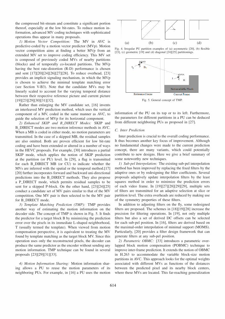
3) Template Matching Prediction (TMP): TMP providesanother way of estimating the motion information on thedecoder side. The concept of TMP is shown in Fig. 5. It findsthe predictor for a target block B by minimizing the predictionerror over the pixels in its immediate L-shaped neighborhood,T (usually termed the template). When viewed from motioncompensation perspective, it is equivalent to treating the MVfound by template matching as the target block MV. Since thisoperation uses only the reconstructed pixels, the decoder canproduce the same predictor as the encoder without sending anymotion information. TMP technique can be found in severalproposals [23][29][31][33].

4) Motion Information Sharing: Motion information shar-ing allows a PU to reuse the motion parameters of itsneighboring PUs. For example, in [16] a PU uses the motion

(a) (b) (c) (d)

Fig. 4. Irregular PU partition examples of (a) asymmetric [20], (b) flexible[23], (c) geometric [19] and (d) diagonal [24][25] partitionings.

Fig. 5. General concept of TMP.

information of the PU on its top or to its left. Furthermore,the parameters for different partitions in a PU can be deducedfrom different neighboring PUs as proposed in [27].

C. Inter Prediction

Inter prediction is crucial to the overall coding performance.It thus becomes another key focus of improvement. Althoughno fundamental changes were made to the current predictionconcept, there are many variants, which could potentiallycontribute to new designs. Here we give a brief summary ofsome noteworthy new techniques.1) Sub-pel Interpolation: The existing sub-pel interpolation

method has been improved by replacing the fixed filters by theadaptive ones or by redesigning the filter coefficients. Severalproposals adaptively update interpolation filters by the leastsquares method in order to minimize the prediction errorsof each video frame. In [19][27][28][29][29], multiple setsof filters are transmitted for an adaptive selection at slice orpartition level. The extra overheads are reduced by making useof the symmetry properties of these filters.In addition to adjusting filters on the fly, some redesigned

filters are proposed. The schemes in [18][19][28] increase theprecision for filtering operations. In [19], not only multiplefilters but also a set of derived DC offsets can be selectedfor each sub-pel position. In [16], filters are derived based onthe maximal-order interpolation of minimal support (MOMS).Particularly, [20] provides a filter design framework that cangenerate filters at any sub-pel position.2) Parametric OBMC: [33] introduces a parametric over-

lapped block motion compensation (POBMC) technique toimprove inter-frame prediction. It extends the notion of OBMCin H.263 to accommodate the variable block-size motionpartitions in AVC. This approach looks for the optimal weightsassociated with different MVs as functions of the distancesbetween the predicted pixel and its nearby block centers,where these MVs are located. This far-reaching generalization

614

provides a generic reconstruction framework, allowing theMVs associated with multiple motion partitions of arbitraryshape to be optimally constructed for motion compensation.

3) Adaptive MV Precision: In AVC, the MV resolution isfixed at 1/4-pel precision. Although a higher precision suchas 1/8-pel [34] can further reduce prediction error, sometimesthe bit-rate increase outweighs the prediction performance dueto additional MV coding overheads. Some HEVC proposalssignal the MV precisions in order to strike a balance betweenmotion accuracy and MV coding bits. In [16], the MV preci-sion is adaptive at the slice level. Moreover, the MV precisionis signaled per MV in [19][20].

4) Weighted Prediction and Illumination Compensation:Weighted prediction performs a linear operation on the pre-dictor, usually with an DC offset, to generate a better predic-tion result. In [24], the weighted prediction coefficients areswitchable for each CU. In [8][21], a new offset is generatedby subtracting the average value of the coded picture fromthat of the reference picture. In [23][30], the luma values ofcurrent block are compensated by the difference between theaverage of neighboring samples of the current block and thatof the reference block.

5) Spatial-temporal prediction: In [23], inter predictionresidual is compensated through intra prediction. The intraprediction reference is generated by the difference betweenthe current and the reference blocks’ neighboring pixels.

D. Intra Prediction

The AVC intra prediction tool provides DC and severaldirectional modes for predicting variable-size blocks. Thepredictor is linearly generated from target block’s neighboringL-shaped coded pixels. However, this prediction scheme hasseveral inherent weaknesses: (a) Poor performance inevitablyincurs when the distances between the reference and thepredicted pixels increase. (b) The straightforward design ofextrapolation filters is incapable of synthesizing periodical andcomplex textures. (c) Artificial edges, which are not usuallyseen in nature scenes, appear along the directions of intraprediction. Based on the above investigations, many tools areproposed to alleviate these problems.

1) Line-based Prediction: Since the intra prediction errortends to be larger for farther away pixels, some proposals try tominimize the distance between the reference and target pixels.Line-based predictions, as illustrated in Fig. 6 (a), divide a16×16 block into 1×16, 16×1, 2×8 or 8×2 partitions ratherthan the conventional square partitions and sequentially codeseach partition to ensure that successive partitions can referexactly to its neighboring pixels [23][35]. Another proposal,termed the recursive intra prediction [36], is analogous to[23] except that the successive partitions are extrapolated byreferring to the predictor of its preceding partition, and only1×16 and 16×1 partitions are available.

2) Pyramid and Interleaved Prediction: The block-basedpyramid prediction [24] firstly encodes a down-sampled ver-sion of the current block, which will then be reconstructed

and upsampled to serve as the final predictor. The resample-based intra prediction [23] encodes an interleaved block shownin Fig. 6 (b). The A-pels in a block are coded first. Then,the predictors of B- and C-pels are formed by referring tothe reconstructed A-pels. After A-, B- and C-pels in a blockare coded, the D-pels can be predicted from all of theirsurrounding pixels.3) Template Matching Average: The TMP technique can

also be applied to the intra frames as show in Fig. 6 (c),aiming at predicting the periodical and the complex tex-tures. To further reduce the estimation error variance, thetemplate matching average (TMA) [27][37] averages the firstN candidate blocks that have the lowest template predictionerrors, to form the predictor. In the line-based TMA [35] thetarget block is degenerated into a straight line. Then TMPis performed on each target line whose coding result can beused afterwards in the prediction of successive target lines.In [20], the pixel-based recursive template matching (PTM) isemployed recursively for each target pixel in the block in theraster-scan order. In addition to the coded pixels in the searchrange, the predicted pixels are included in the template as thesuccessive target pixels.4) Pre- and Post-filtering: The directional patterns of AVC

intra prediction extrapolate directional textures by referring tothe coded neighboring pixels. However, the synthesized texturemay contain artificial edges along the direction perpendicularto the selected prediction direction. The pre- and post-filteringprocesses are thus introduced respectively for reference sam-ples and predictors to alleviate this problem.The pre-filtering process, specified in the AVC High Profile,

employs a low-pass filter on the reference samples prior to theintra 8×8 prediction. The method in [16] extends this pre-filtering process to all partitions except for the intra 4×4.On the other hand, many post-filter processes are proposed.The initial predictor is filtered by a separable 3×3 Gaussiankernel in [36] and by an average filter applied to the currentand neighboring pixels in [20]. The block-based post-filteringis done by a weighted sum of the initial predictor and theneighboring coded blocks in [29]. Yet in [17] the leakyprediction is formed by a weighted sum of the initial predictorand the original block.

5) Plane Prediction: The plane mode prediction, whichaims at producing smoothly-varying textures, is also improved.In [18] the bottom-right most pixel is signaled explicitly tolinearly interpolate the right-most and bottom pixels. Therest pixels are then interpolated bi-linearly. In [25], firstlya 3D plane surface is derived from fitting the values of theneighboring reconstructed pixels P0 in Fig. 6 (d). Then thepredictor of current block P1 is created from fitting its pixelvalues to this surface.

6) Chroma prediction: In general, there should be no cor-relation between luma and chroma values, whereas this is nottrue for the textural regions whose segmentation informationinferred from the luma component can be used for improvingthe chroma prediction. A modified DC mode for chromaprediction [20] exploits the segmentation information from

615

a down-sampled luma block, which is previously coded, toseparate the corresponding chroma block into two irregularparts. The luma segmentation map is generated by the thresh-olding method using the DC mean value. After that, each partis independently estimated by averaging the reference pixelswithin the same segmented region.

7) Extended Directional Prediction: Because the 8 direc-tional modes defined in AVC may not sufficiently represent allpossible directional patterns, various approaches are proposedto increase the number of prediction directions. One is simplyincreasing the number of directions, which delineate the finergranularity in producing a more precise estimation of direc-tional patterns [17][18][20]. Another proposal, as shown inFig. 6 (e), is to find a vector with the largest magnitude of the2-norm of the gradient field constructed from the neighboringreconstructed blocks. The isophotal direction perpendicularto the chosen vector indicates a special directional mode,which shares the same mode number with the DC mode, andwill take effect only if its magnitude exceeds a pre-definedthreshold [27]. The bi-directional intra prediction (BIP) [21]deduces the predictor from averaging the prediction resultsof two different modes. Moreover, in anticipation of furtherimproving the predictive coding efficiency, the coding orderof BIP is changed in the order as depicted in Fig. 6 (f);hence, additional references at the bottom and/or right sidesare available for A, B and C.

E. Transform Coding

The transform coding converts inter/intra prediction resid-uals to the frequency domain in order to decorrelate andcompact the residual signals. However, the DCT basis is notoptimal for various directional patterns in residual signals. Thetransform basis should be made adaptable to the statisticalvariation of realizations. Therefore, anticipation of a needfor better transform coding tools leads to redesigning theexisting DCT-based coding for further optimizing the energycompaction of residual signals.

1) Mode-dependent Directional Transform: The mode-dependent directional transform (MDDT) [38] is widely usedin many HEVC proposals since it has been proven to be ef-fective for decorrelating the redundancies along the directionsof intra prediction. In MDDT, each intra prediction mode iscoupled with an unique pair of transform matrices, whichis derived from the off-line training processes of Karhunen-Loéve transform (KLT), for the strongly mode-dependentresidual signals. In order to lower the hardware cost, theorthogonal MDDT [39] forces the column and row transformmatrices to be the same in the training processes. This slightchange can save half of hardware area or memory usage.However, even for a given intra prediction mode, the

residual signals still have different statistics. Hence, multiplepairs of transform matrices[23][27] [29] are used for a singleintra prediction mode as an enhancement to MDDT. Basedon KLT, each pair of matrices is off-line trained from asubdivision of mode-dependent residual signals. In addition,DCT could be included as another option besides multiple

(a) (b)

(c) (d)

(e) (f)

Fig. 6. (a) 16×1 line-based prediction (diagonal down-left mode) [23][35], (b)resample-based intra prediction [23], (c) template matching intra prediction[37], (d) parametric planar prediction and iterative prediction [25], (e) edge-based directional prediction [27] and (f) prediction order of BIP [21].

transform matrices. Moreover, this approach can be furtherextended for inter block transform coding [23][27].2) Rotational Transform: The rotational transform (ROT)

[20] chooses to change the DCT basis rather than to train anew KLT basis. The energy of residual signals is generallyconcentrated on low-frequency bands after the DCT. Due tothe consideration on complexity, the ROT works only on thecorresponding DCT basis of top-left 8×8 low-frequency bandsof all various partitions, excluding blocks smaller than 16×16.To fit these DCT bases to a certain directional residual pattern,the coordinate system of basis is rotated by two 3D-rotationmatrices for row and column transforms, where each matrix isdefined by three angles for each axis in 3D Euclidean space.

F. Quantization

One element of controlling the quantization process in AVCis the quantization weighting matrix. This matrix can be eitheruniquely defined and sent to the decoder as coding parameters,or substituted by a default one. To match the statistics ofthe transform coefficient distribution, adaptive selection of thequantization weighting matrix is proposed in [21][23].

G. In-loop Filter

In AVC, a deblocking filter is applied to each decodedpicture, before it goes into the decoded picture buffer (DPB),

616

to reduce blocking artifacts. The filter strength is adaptivelyadjusted according to the boundary strength. The proposalsin [18][36] simplify the deblocking filter complexity. Further-more, adaptive loop filters (ALFs) and de-banding algorithmsare introduced to improve the quality of decoded pictures.

1) Adaptive Loop Filter: ALF is applied after the deblock-ing filter by using the Weiner filtering technique, which issimilar to that in Section V-C1, to minimize the MSE betweenthe coded and the original pictures. How to balance the bits forrepresenting filter coefficients and the coding performance, aswell as how to make proper on-off decision of filtering remainto be research problems. Therefore, various ALF schemes havebeen proposed.The main idea of Quad-tree ALF (QALF) is to signal the on-

off decision of filtering through a quad-tree partition process.QALF is adopted, and improved by providing multiple fil-ters for adaptation, as suggested by many HEVC proposals[16][19][27][29][36]. In [20], the decision partition is directlyderived for each CU and the partition can be merged, and asa result only the merged level is signaled.

2) De-banding: Two de-banding processes are proposed by[20]. The first one is applied after the normal deblocking filterin which offsets are sent for each group with pixels havingsimilar edge strengths. The other one is applied after the ALFin which offsets are sent for each pixel group categorized byluma intensities. Conceptually the first de-banding process isfor retaining edge strength and the other one is for matchingthe probability density function between the original and thecoded pictures.

H. Entropy Coding

Although CABAC is proven to be efficient in AVC, it isdesigned for serial processing and its context adaptive featureis based on the statistics of previously coded data. A lowdata throughput is unavoidable and becomes a bottleneck onhandling high resolution videos. Therefore, a new design forentropy encoder should consider parallelism, load-balance andcomplexity/performance tradeoffs.

1) Parallel Capabilities: The parallel processing capabil-ities of CABAC are improved in three aspects, listed fromlarge to small: entropy-slice-level, syntax-level and bin-levelparallelism.The entropy slice-level parallelization [39][40] splits a

frame into several interleaved entropy slices, which maintainand update their own context model (see Fig. 7 (a)). Slice0 should be encoded at least one block earlier than Slice 1,so that the reference blocks for the current block (the whiteblock) are always available.Syntax-level parallelization [39] optimizes the loadings be-

tween multiple and independent entropy coders. It classifiesall the syntax elements into several groups depending on thedegree of parallelization. Since the syntax bit-rate varies fordifferent QPs, the classification is adaptive to the QP value tokeep a good load-balance.Bin-level parallelization [16][41] is a concept of pipelining

the coding process of incoming bin sequences. As shown

(a)

(b)

Fig. 7. (a) An example for the interleaving of two entropy slices [39]. (b) Thebin-level parallelization [16][41].

in Fig. 7 (b), the incoming bins, which are binarized syn-tax elements, are demultiplexed and fed into one of thebin encoders based on the selected context model. The binencoders encode bins into codewords, which will be thenmultiplexed into a bitstream. Moreover, the bin encoder can beimplemented by any entropy encoding methods. For example,the probability interval partitioning entropy (PIPE) coder [16]uses V2V coding (see Section V-H3) as its bin encoders.And experiment shows a significant time saving while onlya negligible additional overhead is paid as compared withCABAC.2) CAVLC: In AVC baseline profile, the non-residual in-

formation is coded by the Exp-Golomb entropy coder whichhas no context adaptive features. Therefore, [18] proposes aCAVLC design for both residual and non-residual informa-tion with two major features. One is to improve the codingefficiency by providing more VLC tables. The other is toimprove the context adaptivity by maintaining a sorting table.In CAVLC, each input is associated with a code number,which decides the corresponding VLC table. The sorting tableis updated according to the probability distributions of codenumbers on the fly. So, the frequent code numbers have VLCtables with shorter codewords.3) Variable-to-Variable Length (V2V) Coding: Compared

with the binary arithmetic coding, the V2V coding [16][41]has the advantage of low complexity without losing codingperformance. Since a bin, 0 or 1, is assigned with a probabilityfrom the context model, a corresponding Huffman table forvariable-length sequences is constructed dynamically. Then,the coding process is only a matter of table look-up.4) Adaptive Coefficient Scanning: The quantized coeffi-

cients for each TU are zig-zag scanned in AVC for theproceeding entropy coding. To better represent of the locationsof the non-zero coefficients, multiple pre-defined scanningorders are provided for selection in [17][19][20][21].

I. Increase Calculation Accuracy

The internal bit-depth increasing (IBDI) [21][26][27] in-creases the calculation precision during the coding process,aiming at reducing the rounding errors in intra prediction,transform and in-loop filtering. For the same purpose, [20]

617

identifies the minimum and the maximum values (Max, Min)of pixels in each slice, then the range [Max, Min] will bescaled to a fixed larger range during the coding process.

VI. CONCLUDING REMARKS

Several international video standards have been developedin the past two decades. They are all based on the motion-compensated transform coding framework. Several attemptshave been made to invent new coding structures. During theMPEG scalable coding competition in 2004, the interframewavelet schemes were suggested. Although the wavelet-basedschemes have a more flexible scalable coding capability, itsvisual quality is slightly inferior. In the past 8 or so years,many researchers look for alternative coding schemes (otherthan the hybrid coding scheme); however, for compressingnatural images, the old motion-compensated transform codingstructure could still be improved and stood out in competi-tion. A clear cost of the improved performance is the hugecomputational complexity.Recently, the compressive sampling (or compressed sensing)

[42] got a lot of attentions. This technique has shown someadvantages in image recognition and reconstruction. However,its advantages in image compression are still under investiga-tion. Do we hit the Shannon limit in terms of image/videocoding? Is HEVC the end of video compression research?Many researchers should be interested in knowing the answers.

ACKNOWLEDGEMENT

This work was supported in part by the NSC, Taiwan underGrants 98-2622-8-009-011 and 98-2219-E-009-015.

REFERENCES

[1] H.-M. Hang and J. W. Woods, Handbook for Visual Communications.Academic Press, 1995.

[2] K. R. Rao and J. J. Hwang, Techniques and for Image, Video, and AudioCoding. Prentice-Hall, 1996.

[3] Y. Q. Shi and H. Sun, Image and Video Compression for MultimediaEngineering. CRC Press, second ed., 2008.

[4] I. E. Richardson, H.264 and MPEG-4 Video Compression: Video Codingfor Next Generation Multimedia. Wiley, 2003.

[5] C. SGXV, “Description of Reference Model 8 (RM8),” Working PartyXV/4, Specialists Group on Coding for Visual Telephony, June 1989.

[6] T. Wiegand, H. Schwarz, A. Joch, F. Kossentini, and G. J. Sullivan,“Rate-constrained coder control and comparison of video coding stan-dards,” IEEE Trans. on Circuits and Systems for Video Technology,vol. 13, pp. 688–703, July 2003.

[7] “Report of the Formal Verification Tests on AVC,” ISO/IECJTC1/SC29/WG11, MPEG03/N6231, December 2003.

[8] “JM11.0KTA2.7.” http://iphome.hhi.de/suehring/tml/download/KTA/.[9] “Vision, Applications and Requirements for High-Performance Video

Coding,” ISO/IEC JTC1/SC29/WG11, MPEG09/N11096, July 2009.[10] J. Ostermann and M. Narroschke, “Draft Requirements for Next-

Generation Video Coding Project,” ITU-T Q.6/SG16, VCEG-AL96, July2009.

[11] “Joint Call for Proporsals on Video Compression Technology,” ISO/IECJTC1/SC29/WG11, MPEG09/N11113, January 2010.

[12] S. Pateux, “Tools for proposal evaluations,” ISO/IEC JTC1/SC29/WG11,JCTVC-A031, April 2010.

[13] “Report of Subjective Test Results of Responses to the Joint Call forProposals (CfP) on Video Coding Technology for High Efficiency VideoCoding,” ISO/IEC JTC1/SC29/WG11, MPEG10/N11275, April 2010.

[14] “Test Model under Consideration,” ISO/IEC JTC1/SC29/WG11, JCTVC-B205, July 2010.

[15] F. Bossen, “Common test conditions and software reference configura-tions,” ISO/IEC JTC1/SC29/WG11, JCTVC-B300, July 2010.

[16] M. Winken and et al., “Description of video coding technology proposalby Fraunhofer HHI,” ISO/IEC JTC1/SC29/WG11, JCTVC-A116, April2010.

[17] T. Davies, “BBC’s Response to the Call for Proposals on VideoCompression Technology,” ISO/IEC JTC1/SC29/WG11, JCTVC-A125,April 2010.

[18] K. Ugur and et al., “Description of video coding technology proposal byTandberg, Nokia, Ericsson,” ISO/IEC JTC1/SC29/WG11, JCTVC-A119,April 2010.

[19] M. Karczewicz and et al., “Video coding technology proposal byQualcomm Inc.,” ISO/IEC JTC1/SC29/WG11, JCTVC-A121, April 2010.

[20] K. McCann and et al., “Samsung’s Response to the Call for Proposals onVideo Compression Technology,” ISO/IEC JTC1/SC29/WG11, JCTVC-A124, April 2010.

[21] T. Chujoh and et al., “Description of video coding technology proposalby TOSHIBA,” ISO/IEC JTC1/SC29/WG11, JCTVC-A117, April 2010.

[22] “JM16.2.” http://iphome.hhi.de/suehring/tml/download/.[23] H. Yang and et al., “Description of video coding technology pro-

posal by Huawei Technologies and Hisilicon Technologies,” ISO/IECJTC1/SC29/WG11, JCTVC-A111, April 2010.

[24] K. Sugimoto and et al., “Description of video coding technologyproposal by Mitsubishi Electric,” ISO/IEC JTC1/SC29/WG11, JCTVC-A107, April 2010.

[25] A. Ichigaya and et al., “Description of video coding technology proposalby NHK and Mitsubishi,” ISO/IEC JTC1/SC29/WG11, JCTVC-A122,April 2010.

[26] K. Chono and et al., “Description of video coding technology proposalby NEC Corp.,” ISO/IEC JTC1/SC29/WG11, JCTVC-A104, April 2010.

[27] I. Amonou and et al., “Description of video coding technology proposalby France Telecom, NTT, NTT DOCOMO, Panasonic and Technicolor,”ISO/IEC JTC1/SC29/WG11, JCTVC-A114, April 2010.

[28] T. Suzuki and A. Tabatabai, “Description of video coding technologyproposal by Sony,” ISO/IEC JTC1/SC29/WG11, JCTVC-A103, April2010.

[29] Y.-W. Huang and et al., “A Technical Description of MediaTek’sProposal to the JCT-VC CfP,” ISO/IEC JTC1/SC29/WG11, JCTVC-A109, April 2010.

[30] B. Jeon and et al., “Description of video coding technology proposal byLG Electronics,” ISO/IEC JTC1/SC29/WG11, JCTVC-A110, April 2010.

[31] S. Kamp and M. Wien, “Description of video coding technologyproposal by RWTH Aachen University,” ISO/IEC JTC1/SC29/WG11,JCTVC-A112, April 2010.

[32] J. Lim and et al., “Description of video coding technology proposalby SK telecom, Sejong Univ. and Sungkyunkwan Univ.,” ISO/IECJTC1/SC29/WG11, JCTVC-A113, April 2010.

[33] Y.-W. Chen and et al., “Description of video coding technology proposalby NCTU,” ISO/IEC JTC1/SC29/WG11, JCTVC-A123, April 2010.

[34] J. Ostermann and M. Narroschke, “Motion compensated prediction with1/8-pel displacement vector resolution,” ITU-T Q.6/SG16, VCEG-AD09,October 2006.

[35] F. Wu and et al., “Description of video coding technology proposal byMicrosoft,” ISO/IEC JTC1/SC29/WG11, JCTVC-A118, April 2010.

[36] H. Y. Kim and et al., “Description of video coding technology proposalby ETRI,” ISO/IEC JTC1/SC29/WG11, JCTVC-A127, April 2010.

[37] T. K. Tan, C. S. Boon, and Y. Suzuki, “Intra Prediction by AveragedTemplate Matching Predictors,” IEEE Proc. of Consumer Communica-tions and Networking Conference, January 2007.

[38] Y. Ye and M. Karczewicz, “Improved H.264 Intra Coding based onBi-directional Intra Prediction, Directional Transform, and AdaptiveCoefficient Scanning,” IEEE Int’l Conference on Image Processing,December 2008.

[39] M. Budagavi and et al., “Description of video coding technology pro-posal by Texas Instruments Inc.,” ISO/IEC JTC1/SC29/WG11, JCTVC-A101, April 2010.

[40] A. Segall and et al., “A Highly Efficient and Highly Parallel System forVideo Coding,” ISO/IEC JTC1/SC29/WG11, JCTVC-A105, April 2010.

[41] D. He and et al., “Video Coding Technology Proposal by RIM,” ISO/IECJTC1/SC29/WG11, JCTVC-A120, April 2010.

[42] V. K. Goyal, A. K. Fletcher, and S. Rangan, “Compressive sampling andlossy compression,” IEEE Signal Processing Magazine, vol. 25, pp. 48–56, March 2008.

618