towards using unlabeled data in a sparse-coding framework for
TRANSCRIPT

Towards Using Unlabeled Data in a Sparse-coding Framework for Human Activity Recognition
Sourav Bhattacharyaa, Petteri Nurmia, Nils Hammerlab, and Thomas Plötzb
aHelsinki Institute for Information Technology HIIT, Department of Computer Science, University of Helsinki, Finland
bCulture Lab, School of Computing Science, Newcastle University, UK “NOTICE: this is the author’s version of a work that was accepted for publication in Pervasive and Mobile Computing. Changes resulting from the publishing process, such as peer review, editing, corrections, structural formatting, and other quality control mechanisms may not be reflected in this document. Changes may have been made to this work since it was submitted for publication. DOI: 10.1016/j.pmcj.2014.05.006”
arX
iv:1
312.
6995
v3 [
cs.L
G]
23
Jul 2
014

Towards Using Unlabeled Data in a Sparse-coding Framework for Human ActivityRecognition
Sourav Bhattacharyaa, Petteri Nurmia, Nils Hammerlab, Thomas Plotzb
aHelsinki Institute for Information Technology HIITDepartment of Computer Science, University of Helsinki, Finland
bCulture Lab, School of Computing Science, Newcastle University, UK
Abstract
We propose a sparse-coding framework for activity recognition in ubiquitous and mobile computing that alleviates twofundamental problems of current supervised learning approaches. (i) It automatically derives a compact, sparse andmeaningful feature representation of sensor data that does not rely on prior expert knowledge and generalizes wellacross domain boundaries. (ii) It exploits unlabeled sample data for bootstrapping effective activity recognizers, i.e.,substantially reduces the amount of ground truth annotation required for model estimation. Such unlabeled data is easyto obtain, e.g., through contemporary smartphones carried by users as they go about their everyday activities.
Based on the self-taught learning paradigm we automatically derive an over-complete set of basis vectors from un-labeled data that captures inherent patterns present within activity data. Through projecting raw sensor data onto thefeature space defined by such over-complete sets of basis vectors effective feature extraction is pursued. Given theselearned feature representations, classification backends are then trained using small amounts of labeled training data.
We study the new approach in detail using two datasets which differ in terms of the recognition tasks and sensormodalities. Primarily we focus on a transportation mode analysis task, a popular task in mobile-phone based sens-ing. The sparse-coding framework demonstrates better performance than the state-of-the-art in supervised learningapproaches. More importantly, we show the practical potential of the new approach by successfully evaluating its gen-eralization capabilities across both domain and sensor modalities by considering the popular Opportunity dataset. Ourfeature learning approach outperforms state-of-the-art approaches to analyzing activities of daily living.
Keywords: Activity Recognition, Sparse-coding, Machine Learning, Unsupervised Learning.
1. Introduction
Activity recognition represents a major research areawithin mobile and pervasive/ubiquitous computing [1, 3].Prominent examples of domains where activity recogni-tion has been investigated include smart homes [4, 5, 6],situated support [7], automatic monitoring of mental andphysical wellbeing [8, 9, 10], and general health care [11,12]. Modern smartphones with their advanced sensingcapabilities provide a particularly attractive platform foractivity recognition as they are carried around by manypeople while going about their everyday activities.
The vast majority of activity recognition research re-lies on supervised learning techniques where handcraftedfeatures, e.g., heuristically chosen statistical measures,are extracted from raw sensor recordings, which are thencombined with activity labels for effective classifier train-ing. While this approach is in line with the standard
procedures in many application domains of general pat-tern recognition and machine learning techniques [13], itis often too costly or simply not applicable for ubiqui-tous/pervasive computing applications. The reasons forthis are twofold. Firstly, the performance of supervisedlearning approaches is highly sensitive to the type of fea-ture extraction, where often the optimal set of featuresvaries across different activities [14, 15, 16]. Secondly,and more crucially, obtaining reliable ground truth anno-tation for bootstrapping and training activity recognizersposes a challenge for system developers who target real-world deployments. People typically carry their mobiledevice while going about their everyday activities, therebynot paying much attention to the phone itself in terms oflocation of the device (in the pocket, in the backpack, etc.)and only sporadically interacting with it (for making a callor explicitly using the device’s services for, e.g., informa-
Preprint submitted to Pervasive and Mobile Computing July 24, 2014

tion retrieval). Consequently, active support from users toprovide labels for data collected in real-life scenarios can-not be considered feasible for many settings as promptingmobile phone users to annotate their activities while theyare pursuing them has its limitations. Apart from theselimitations, privacy and ethical considerations typicallyrender direct observation and annotation impracticable inrealistic scenarios.
Possible alternatives to such direct observation and an-notation include: (i) self-reporting of activities by theusers, e.g., using a diary [17]; (ii) the use of experiencesampling, i.e., prompting the user and asking for the cur-rent or previous activity label [4, 18]; and (iii) a combina-tion of these methods. While such techniques somewhatalleviate the aforementioned problem by providing anno-tation for at least smaller subsets of unlabeled data, theystill remain prone to errors and typically cannot replaceexpert ground truth annotation.
Whereas obtaining reliable ground truth annotation ishard to achieve, the collection of, even large amounts of,unlabeled sample data is typically straightforward. Peo-ple’s smartphones can simply record activity data in anopportunistic way, without requiring the user to follow acertain protocol or scripted activity patterns. This is espe-cially attractive since it allows for capturing sensor datawhile users perform their natural activities without neces-sarily being conscious about the actual data collection.
In this paper we introduce a novel framework for activ-ity recognition. Our approach mitigates the requirementof large amounts of ground truth annotation by explic-itly exploiting unlabeled sensor data for bootstrapping ourrecognition framework. Based on the self-taught learn-ing paradigm [19], we develop a sparse-coding frame-work for unsupervised estimation of sensor data repre-sentations with the help of a codebook of basis vectors(see Section 3.2). As these representations are learnedin an unsupervised manner, our approach also overcomesthe need to perform feature-engineering. While the origi-nal framework of self-taught learning has been developedmainly for the analysis of non-sequential data, i.e., imagesand stationary audio signals [20], we extend the approachtowards time-series data such as continuous sensor datastreams. We also develop a basis selection method thatbuilds on information theory to generate a codebook ofbasis vectors that covers characteristic movement patternsin human physical activities. Using activations of thesebasis vectors (see Section 3.3) we then compute featuresof the raw sensor data streams, which are the basis forsubsequent classifier training. The latter requires only rel-atively small amounts of labeled data, which alleviates the
ground truth annotation challenge of mobile computingapplications.
We demonstrate the benefits of our approach using datafrom two diverse activity recognition tasks, namely trans-portation mode analysis and classification of activities ofdaily living (the Opportunity challenge [21]). Our ex-periments demonstrate that the proposed approach pro-vides better results than the state-of-the-art, namely PCA-based feature learning, semi-supervised En-Co-Training,and feature-engineering based (supervised) algorithms,while requiring smaller amounts of training data and notrelying on prior domain knowledge for feature crafting.Apart from successful generalization across recognitiontasks, we also demonstrate easy applicability of our pro-posed framework beyond modality boundaries coveringnot only accelerometer data but also other commonlyavailable sensors on the mobile platform, such as the gy-roscopes, or magnetometers.
2. Learning From Unlabeled Data
The focus of our work is on developing an effectiveframework that exploits unlabeled data to derive robustactivity recognizers for mobile applications. The key ideais to use vast amounts of easy to record unlabeled sam-ple data for unsupervised feature learning. These featuresshall cover general characteristics of human movements,which guarantees both robustness and generalizability.
Only very little related work exists that focus on incor-porating unlabeled data for training mobile activity rec-ognizers. A notable exception is the work by Amft whoexplored self-taught learning in a very preliminary studyfor activity spotting using on-body motion sensors [22].However, that work does not take into account the proper-ties of the learned codebook which play an important rolein the recognition task.
The idea of incorporating unlabeled data and relatedfeature learning techniques into recognizer training is awell researched area in the general machine learning andpattern recognition community. In the following, we willsummarize relevant related work from these fields and linkthem to the mobile and ubiquitous computing domain.
2.1. Non-supervised Learning Paradigms
A number of general learning paradigms have been de-veloped that focus on deriving statistical models and rec-ognizers by incorporating unlabeled data. Although dif-fering in their particular approaches, all related techniquesshare the objective of alleviating the dependence on a
3

large amount of annotated training data for parameter es-timation.
Learning from a combination of labeled and unlabeleddatasets is commonly known as semi-supervised learn-ing [23]. The most common approach to semi-supervisedlearning is generative models, where the unknown datadistribution p(x) is modeled as a mixture of class condi-tional distributions p(x|y), where y is the (unobserved)class variable. The mixture components are estimatedfrom a large amount of unlabeled and small amount oflabeled data by applying the Expectation Maximization(EM) algorithm. The predictive estimate of p(y|x) isthen computed using Bayes’ formula. Other approachesto semi-supervised learning include self-training, co-training, transductive SVM (TSVM), graphical modelsand multiview learning.
Semi-supervised learning techniques have also been ap-plied to activity recognition, e.g., for recognizing loco-motion related activities [24], and in smart homes [25]. Inorder to be effective, semi-supervised learning approachesneed to satisfy certain, rather strict assumptions [23, 26].Probably the strongest constraint imposed by these tech-niques is that they assume that the unlabeled and la-beled datasets are drawn from the same distribution, i.e.,Du = Dl. In other words, the unlabeled dataset has tobe collected with strict focus on the set of activities therecognizer shall cover. This limits generalization capabil-ity and renders the learning error-prone for real-world set-tings where the user might perform extraneous activities,or no activity at all [27]. Our approach provides improvedgeneralization capability by relaxing the equality condi-tion for the distributions of unlabeled and labeled datasets,i.e., Du 6= Dl.
An alternative approach to dealing with unlabeled datais active learning. Techniques for active learning aim tomake the most economic use of annotations by identifyingthose unlabeled samples that are most uncertain and thustheir annotation would provide most information for thetraining process. Such samples are automatically iden-tified using information theoretic criteria and then man-ual annotation is requested. Active learning approacheshave become very popular in a number of applicationdomains including activity recognition using body-wornsensors [30, 25]. Active learning operates on pre-definedsets of features, which stands in contrast to our approachthat automatically learns feature representations. In do-ing so, active learning becomes sensitive to the particularfeatures that have been extracted, hence limiting its gen-eralizability.
Explicitly focusing on generalizability of recognition
frameworks, transfer learning techniques have been de-veloped to bridge, e.g., application domains with differ-ing classes or sensing modalities [31]. In this approach,knowledge acquired in a specific domain can be trans-ferred to another, if a systematic transformation is eitherprovided or learned automatically. Transfer learning hasbeen applied to ubiquitous computing problems, for ex-ample, for adapting models learned with data from onesmart home to work within another smart home [32, 33],or to adapt activity classifiers learned with data from oneuser to work with other users [34]. In these approachesthe need for annotated training data is not directly reducedbut shifted to other domains or modalities, which can bebeneficial if such data are easier to obtain.
As an alternative approach to alleviating the demandsof ground truth annotation so-called multi-instance learn-ing techniques have been developed. These techniquesassign labels to sets of instances instead of individual datapoints [35]. Multi-instance learning has also been appliedfor activity recognition tasks in ubiquitous computing set-tings [18, 36]. To apply multi-instance learning, labels ofthe individual instances were considered as hidden vari-ables and a support vector machine was trained to min-imize the expected loss of the classification of instancesusing the labels of the instance sets. Multi-instance learn-ing also operates on a predefined set of features and there-fore has limited generalizability.
2.2. Feature Learning
Exploiting unlabeled data can also be applied at the fea-ture level to derive a compact and meaningful representa-tion of raw input data. In fact, feature learning, i.e., un-supervised estimation of suitable data representations, hasbeen actively researched in the machine learning commu-nity [37]. The goal of feature learning is to identify andmodel interesting regularities in the sensor data withoutbeing driven by class information. The majority of meth-ods rely on a process similar to generative models but em-ploy efficient, approximative learning algorithms insteadof EM [38].
Data representations for activity recognition in theubiquitous or mobile computing domain typically corre-spond to some sort of “engineered” feature sets, e.g., sta-tistical values calculated over analysis windows that areextracted using a sliding window procedure [14]. Suchpredefined features often do not generalize across domainboundaries, which requires system developers to optimizetheir data representation virtually from scratch for everynew application domain.
4

Only recently, concepts of feature learning have beensuccessfully applied for activity recognition tasks. Forexample, Mantyjarvi et al. [39] compared the use of Prin-cipal Component Analysis (PCA) and Independent Com-ponent Analysis (ICA) for extracting features from sensordata. In their approach, either PCA or ICA was applied onraw sensor values. A sliding window was then applied onthe transformed data and a Wavelet-based feature extrac-tion method was used in combination with a multilayerperceptron.
Similarly, Plotz et al. employed principal componentanalysis to derive features from tri-axial accelerometerdata using a sliding window approach [40]. However, in-stead of applying the PCA on the raw sensor values, theyused the empirical cumulative distribution of a data frameto represent the signals before applying PCA [42]. More-over, they investigated the use of Restricted BoltzmannMachines [38], to train an autoencoder network for fea-ture learning.
Minnen et al. [43] considered activities as sparse motifsin multidimensional time series and proposed an unsuper-vised algorithm for automatically extracting such motifsfrom data. A related approach was proposed by Frank etal. [44] who used time-delay embeddings to extract fea-tures from windowed data and fed these features to a sub-sequent classifier.
Contrary to the popular Fourier and Wavelet representa-tions, which suffer from non-adaptability to the particulardataset [45], we employ a data-adaptive approach of rep-resenting accelerometer measurements. The data-adaptiverepresentation is tailored to the statistics of the data andis directly learned from the recorded measurements. Ex-amples of data-adaptive methods include PCA, ICA andMatrix Factorization. Our approach differs from commondata-adaptive methods by employing an over-completeand sparse feature representation technique. Here, over-completeness indicates that the dimension of the featurespace is much higher than the original input data dimen-sion, and sparsity indicates that the majority of the ele-ments in a feature vector is zero.
3. A Sparse-Coding Framework for ActivityRecognition
We propose a sparse-coding framework for activityrecognition that uses a codebook of basis vectors that cap-ture characteristic and latent patterns in the sensor data.As the codebook learning is unsupervised and operates onunlabeled data, our approach effectively reduces the needfor annotated ground truth data and overcomes the need
to use predefined feature representations, rendering ourapproach well suited for continuous activity recognitiontasks under naturalistic settings.
3.1. Method Overview
Figure 1 gives an overview of our approach to learn-ing activity recognizers. We first collect unlabeled data,which in our experiments consists mainly of tri-axial ac-celerometer measurements (upper part of Figure 1(a)). Wethen solve an optimization problem (see Section 3.2) tolearn a set of basis vectors — the codebook — that cap-ture characteristic patterns of human movements as theycan be observed from the raw sensor data (lower part ofFigure 1(a)).
Once the codebook has been learned, we use a small setof labeled data to train an activity classifier (Figure 1(b)).The features that are used for training the classifier cor-respond to so-called activations, which are vectors thatenable transferring sensor readings to the feature spacespanned by the basis vectors in the codebook. Aftermodel training, the activity label for new sensor readingscan be determined by transferring the corresponding mea-surements into the same feature space and applying thelearned classifier.
3.2. Codebook Learning from Unlabeled Data
We consider sequential, multidimensional sensor data,which in our experiments correspond to measurementsfrom a tri-axial accelerometer or a gyroscope. We ap-ply a sliding window procedure on the measurements toextract overlapping, fixed length frames. Specifically, weconsider measurements of the form xi ∈ Rn, where xi isa vector containing all measurements within the ith frameand n is the length of the frame, i.e., the unlabeled mea-surements are represented as the set
X = {x1,x2, . . . ,xK}, xi ∈ Rn. (1)
In the first step of our approach, we use the unlabeleddata X to learn a codebook B that captures latent andcharacteristic patterns in the sensor measurements. Thecodebook consists of S basis vectors {βj}Sj=1, where eachbasis vector βj ∈ Rn represents a particular pattern in thedata. Once the codebook has been learned, any frame ofsensor measurements can be represented as a linear super-position of the basis vectors, i.e.,
xi ≈S∑j=1
aijβj , (2)
5
Unlabeled data
10 20 30 40 50 60 70 80 90 100
-0.5
0
0.5
B 1
10 20 30 40 50 60 70 80 90 100
-0.5
0
0.5
B 2
10 20 30 40 50 60 70 80 90 100
-0.5
0
0.5
B 3
10 20 30 40 50 60 70 80 90 100
-0.5
0
0.5
B 4
10 20 30 40 50 60 70 80 90 100
-0.5
0
0.5
B 5
10 20 30 40 50 60 70 80 90 100
-0.5
0
0.5
B 6
10 20 30 40 50 60 70 80 90 100
-0.5
0
0.5
B 7
10 20 30 40 50 60 70 80 90 100
-0.5
0
0.5
B 8
10 20 30 40 50 60 70 80 90 100
-0.5
0
0.5
B 9
10 20 30 40 50 60 70 80 90 100
-0.5
0
0.5
B 10
10 20 30 40 50 60 70 80 90 100
-0.5
0
0.5
B 11
10 20 30 40 50 60 70 80 90 100
-0.5
0
0.5
B 12
10 20 30 40 50 60 70 80 90 100
-0.5
0
0.5
B 13
10 20 30 40 50 60 70 80 90 100
-0.5
0
0.5
B 14
10 20 30 40 50 60 70 80 90 100
-0.5
0
0.5
B 15
10 20 30 40 50 60 70 80 90 100
-0.5
0
0.5
B 16
10 20 30 40 50 60 70 80 90 100
-0.5
0
0.5
B 17
10 20 30 40 50 60 70 80 90 100
-0.5
0
0.5
B 18
10 20 30 40 50 60 70 80 90 100
-0.5
0
0.5
B 19
10 20 30 40 50 60 70 80 90 100
-0.5
0
0.5
B 20
10 20 30 40 50 60 70 80 90 100
-0.5
0
0.5
B 21
10 20 30 40 50 60 70 80 90 100
-0.5
0
0.5
B 22
10 20 30 40 50 60 70 80 90 100
-0.5
0
0.5
B 23
10 20 30 40 50 60 70 80 90 100
-0.5
0
0.5
B 24
10 20 30 40 50 60 70 80 90 100
-0.5
0
0.5
B 25
10 20 30 40 50 60 70 80 90 100
-0.5
0
0.5
B 26
10 20 30 40 50 60 70 80 90 100
-0.5
0
0.5
B 27
10 20 30 40 50 60 70 80 90 100
-0.5
0
0.5
B 28
10 20 30 40 50 60 70 80 90 100
-0.5
0
0.5
B 29
10 20 30 40 50 60 70 80 90 100
-0.5
0
0.5
B 30
10 20 30 40 50 60 70 80 90 100
-0.5
0
0.5
B 31
10 20 30 40 50 60 70 80 90 100
-0.5
0
0.5
B 32
10 20 30 40 50 60 70 80 90 100
-0.5
0
0.5
B 33
10 20 30 40 50 60 70 80 90 100
-0.5
0
0.5
B 34
10 20 30 40 50 60 70 80 90 100
-0.5
0
0.5
B 35
10 20 30 40 50 60 70 80 90 100
-0.5
0
0.5
B 36
10 20 30 40 50 60 70 80 90 100
-0.5
0
0.5
B 37
10 20 30 40 50 60 70 80 90 100
-0.5
0
0.5
B 38
10 20 30 40 50 60 70 80 90 100
-0.5
0
0.5
B 39
10 20 30 40 50 60 70 80 90 100
-0.5
0
0.5
B 40
10 20 30 40 50 60 70 80 90 100
-0.5
0
0.5
B 41
10 20 30 40 50 60 70 80 90 100
-0.5
0
0.5
B 42
10 20 30 40 50 60 70 80 90 100
-0.5
0
0.5
B 43
10 20 30 40 50 60 70 80 90 100
-0.5
0
0.5
B 44
10 20 30 40 50 60 70 80 90 100
-0.5
0
0.5
B 45
10 20 30 40 50 60 70 80 90 100
-0.5
0
0.5
B 46
10 20 30 40 50 60 70 80 90 100
-0.5
0
0.5
B 47
10 20 30 40 50 60 70 80 90 100
-0.5
0
0.5
B 48
10 20 30 40 50 60 70 80 90 100
-0.5
0
0.5
B 49
10 20 30 40 50 60 70 80 90 100
-0.5
0
0.5
B 50
10 20 30 40 50 60 70 80 90 100
-0.5
0
0.5
B 51
10 20 30 40 50 60 70 80 90 100
-0.5
0
0.5
B 52
10 20 30 40 50 60 70 80 90 100
-0.5
0
0.5
B 53
10 20 30 40 50 60 70 80 90 100
-0.5
0
0.5
B 54
10 20 30 40 50 60 70 80 90 100
-0.5
0
0.5
B 55
10 20 30 40 50 60 70 80 90 100
-0.5
0
0.5
B 56
10 20 30 40 50 60 70 80 90 100
-0.5
0
0.5
B 57
10 20 30 40 50 60 70 80 90 100
-0.5
0
0.5
B 58
10 20 30 40 50 60 70 80 90 100
-0.5
0
0.5
B 59
10 20 30 40 50 60 70 80 90 100
-0.5
0
0.5
B 60
10 20 30 40 50 60 70 80 90 100
-0.5
0
0.5
B 61
10 20 30 40 50 60 70 80 90 100
-0.5
0
0.5
B 62
10 20 30 40 50 60 70 80 90 100
-0.5
0
0.5
B 63
10 20 30 40 50 60 70 80 90 100
-0.5
0
0.5
B 64
10 20 30 40 50 60 70 80 90 100
-0.5
0
0.5
B 1
10 20 30 40 50 60 70 80 90 100
-0.5
0
0.5
B 2
10 20 30 40 50 60 70 80 90 100
-0.5
0
0.5
B 3
10 20 30 40 50 60 70 80 90 100
-0.5
0
0.5
B 4
10 20 30 40 50 60 70 80 90 100
-0.5
0
0.5
B 5
10 20 30 40 50 60 70 80 90 100
-0.5
0
0.5
B 6
10 20 30 40 50 60 70 80 90 100
-0.5
0
0.5
B 7
10 20 30 40 50 60 70 80 90 100
-0.5
0
0.5
B 8
10 20 30 40 50 60 70 80 90 100
-0.5
0
0.5
B 9
10 20 30 40 50 60 70 80 90 100
-0.5
0
0.5
B 10
10 20 30 40 50 60 70 80 90 100
-0.5
0
0.5
B 11
10 20 30 40 50 60 70 80 90 100
-0.5
0
0.5
B 12
10 20 30 40 50 60 70 80 90 100
-0.5
0
0.5
B 13
10 20 30 40 50 60 70 80 90 100
-0.5
0
0.5
B 14
10 20 30 40 50 60 70 80 90 100
-0.5
0
0.5
B 15
10 20 30 40 50 60 70 80 90 100
-0.5
0
0.5
B 16
10 20 30 40 50 60 70 80 90 100
-0.5
0
0.5
B 17
10 20 30 40 50 60 70 80 90 100
-0.5
0
0.5
B 18
10 20 30 40 50 60 70 80 90 100
-0.5
0
0.5
B 19
10 20 30 40 50 60 70 80 90 100
-0.5
0
0.5
B 20
10 20 30 40 50 60 70 80 90 100
-0.5
0
0.5
B 21
10 20 30 40 50 60 70 80 90 100
-0.5
0
0.5
B 22
10 20 30 40 50 60 70 80 90 100
-0.5
0
0.5
B 23
10 20 30 40 50 60 70 80 90 100
-0.5
0
0.5
B 24
10 20 30 40 50 60 70 80 90 100
-0.5
0
0.5
B 25
10 20 30 40 50 60 70 80 90 100
-0.5
0
0.5
B 26
10 20 30 40 50 60 70 80 90 100
-0.5
0
0.5
B 27
10 20 30 40 50 60 70 80 90 100
-0.5
0
0.5
B 28
10 20 30 40 50 60 70 80 90 100
-0.5
0
0.5
B 29
10 20 30 40 50 60 70 80 90 100
-0.5
0
0.5
B 30
10 20 30 40 50 60 70 80 90 100
-0.5
0
0.5
B 31
10 20 30 40 50 60 70 80 90 100
-0.5
0
0.5
B 32
10 20 30 40 50 60 70 80 90 100
-0.5
0
0.5
B 33
10 20 30 40 50 60 70 80 90 100
-0.5
0
0.5
B 34
10 20 30 40 50 60 70 80 90 100
-0.5
0
0.5
B 35
10 20 30 40 50 60 70 80 90 100
-0.5
0
0.5
B 36
10 20 30 40 50 60 70 80 90 100
-0.5
0
0.5
B 37
10 20 30 40 50 60 70 80 90 100
-0.5
0
0.5
B 38
10 20 30 40 50 60 70 80 90 100
-0.5
0
0.5
B 39
10 20 30 40 50 60 70 80 90 100
-0.5
0
0.5
B 40
10 20 30 40 50 60 70 80 90 100
-0.5
0
0.5
B 41
10 20 30 40 50 60 70 80 90 100
-0.5
0
0.5
B 42
10 20 30 40 50 60 70 80 90 100
-0.5
0
0.5
B 43
10 20 30 40 50 60 70 80 90 100
-0.5
0
0.5
B 44
10 20 30 40 50 60 70 80 90 100
-0.5
0
0.5
B 45
10 20 30 40 50 60 70 80 90 100
-0.5
0
0.5
B 46
10 20 30 40 50 60 70 80 90 100
-0.5
0
0.5
B 47
10 20 30 40 50 60 70 80 90 100
-0.5
0
0.5
B 48
10 20 30 40 50 60 70 80 90 100
-0.5
0
0.5
B 49
10 20 30 40 50 60 70 80 90 100
-0.5
0
0.5
B 50
10 20 30 40 50 60 70 80 90 100
-0.5
0
0.5
B 51
10 20 30 40 50 60 70 80 90 100
-0.5
0
0.5
B 52
10 20 30 40 50 60 70 80 90 100
-0.5
0
0.5
B 53
10 20 30 40 50 60 70 80 90 100
-0.5
0
0.5
B 54
10 20 30 40 50 60 70 80 90 100
-0.5
0
0.5
B 55
10 20 30 40 50 60 70 80 90 100
-0.5
0
0.5
B 56
10 20 30 40 50 60 70 80 90 100
-0.5
0
0.5
B 57
10 20 30 40 50 60 70 80 90 100
-0.5
0
0.5
B 58
10 20 30 40 50 60 70 80 90 100
-0.5
0
0.5
B 59
10 20 30 40 50 60 70 80 90 100
-0.5
0
0.5
B 60
10 20 30 40 50 60 70 80 90 100
-0.5
0
0.5
B 61
10 20 30 40 50 60 70 80 90 100
-0.5
0
0.5
B 62
10 20 30 40 50 60 70 80 90 100
-0.5
0
0.5
B 63
10 20 30 40 50 60 70 80 90 100
-0.5
0
0.5
B 64
Codebook of basis vectors
Unsupervised learning
1 2 3 4
· · ·s
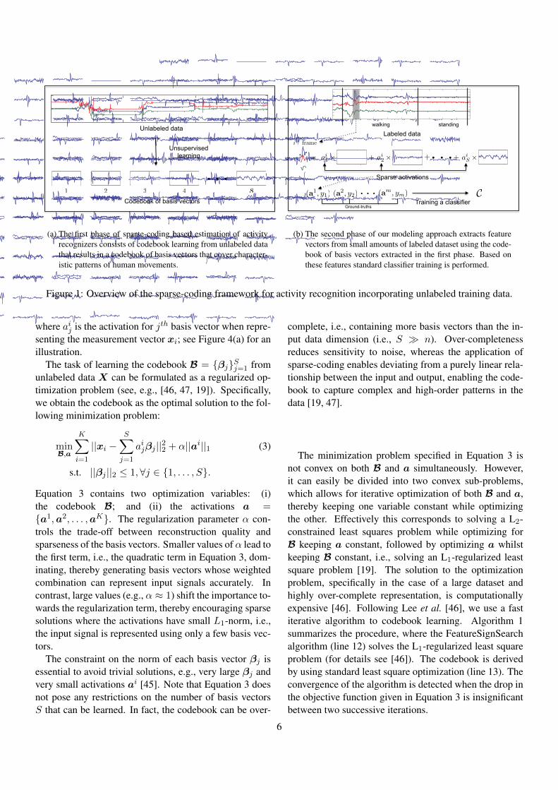
(a) The first phase of sparse-coding based estimation of activityrecognizers consists of codebook learning from unlabeled datathat results in a codebook of basis vectors that cover character-istic patterns of human movements.
Labeled data walking standing
10 20 30 40 50 60 70 80 90 100
-0.5
0
0.5
B 1
10 20 30 40 50 60 70 80 90 100
-0.5
0
0.5
B 2
10 20 30 40 50 60 70 80 90 100
-0.5
0
0.5
B 3
10 20 30 40 50 60 70 80 90 100
-0.5
0
0.5
B 4
10 20 30 40 50 60 70 80 90 100
-0.5
0
0.5
B 5
10 20 30 40 50 60 70 80 90 100
-0.5
0
0.5
B 6
10 20 30 40 50 60 70 80 90 100
-0.5
0
0.5
B 7
10 20 30 40 50 60 70 80 90 100
-0.5
0
0.5
B 8
10 20 30 40 50 60 70 80 90 100
-0.5
0
0.5
B 9
10 20 30 40 50 60 70 80 90 100
-0.5
0
0.5
B 10
10 20 30 40 50 60 70 80 90 100
-0.5
0
0.5
B 11
10 20 30 40 50 60 70 80 90 100
-0.5
0
0.5
B 12
10 20 30 40 50 60 70 80 90 100
-0.5
0
0.5
B 13
10 20 30 40 50 60 70 80 90 100
-0.5
0
0.5
B 14
10 20 30 40 50 60 70 80 90 100
-0.5
0
0.5
B 15
10 20 30 40 50 60 70 80 90 100
-0.5
0
0.5
B 16
10 20 30 40 50 60 70 80 90 100
-0.5
0
0.5
B 17
10 20 30 40 50 60 70 80 90 100
-0.5
0
0.5
B 18
10 20 30 40 50 60 70 80 90 100
-0.5
0
0.5
B 19
10 20 30 40 50 60 70 80 90 100
-0.5
0
0.5
B 20
10 20 30 40 50 60 70 80 90 100
-0.5
0
0.5
B 21
10 20 30 40 50 60 70 80 90 100
-0.5
0
0.5
B 22
10 20 30 40 50 60 70 80 90 100
-0.5
0
0.5
B 23
10 20 30 40 50 60 70 80 90 100
-0.5
0
0.5
B 24
10 20 30 40 50 60 70 80 90 100
-0.5
0
0.5
B 25
10 20 30 40 50 60 70 80 90 100
-0.5
0
0.5
B 26
10 20 30 40 50 60 70 80 90 100
-0.5
0
0.5
B 27
10 20 30 40 50 60 70 80 90 100
-0.5
0
0.5
B 28
10 20 30 40 50 60 70 80 90 100
-0.5
0
0.5
B 29
10 20 30 40 50 60 70 80 90 100
-0.5
0
0.5
B 30
10 20 30 40 50 60 70 80 90 100
-0.5
0
0.5
B 31
10 20 30 40 50 60 70 80 90 100
-0.5
0
0.5
B 32
10 20 30 40 50 60 70 80 90 100
-0.5
0
0.5
B 33
10 20 30 40 50 60 70 80 90 100
-0.5
0
0.5
B 34
10 20 30 40 50 60 70 80 90 100
-0.5
0
0.5
B 35
10 20 30 40 50 60 70 80 90 100
-0.5
0
0.5
B 36
10 20 30 40 50 60 70 80 90 100
-0.5
0
0.5
B 37
10 20 30 40 50 60 70 80 90 100
-0.5
0
0.5
B 38
10 20 30 40 50 60 70 80 90 100
-0.5
0
0.5
B 39
10 20 30 40 50 60 70 80 90 100
-0.5
0
0.5
B 40
10 20 30 40 50 60 70 80 90 100
-0.5
0
0.5
B 41
10 20 30 40 50 60 70 80 90 100
-0.5
0
0.5
B 42
10 20 30 40 50 60 70 80 90 100
-0.5
0
0.5
B 43
10 20 30 40 50 60 70 80 90 100
-0.5
0
0.5
B 44
10 20 30 40 50 60 70 80 90 100
-0.5
0
0.5
B 45
10 20 30 40 50 60 70 80 90 100
-0.5
0
0.5
B 46
10 20 30 40 50 60 70 80 90 100
-0.5
0
0.5
B 47
10 20 30 40 50 60 70 80 90 100
-0.5
0
0.5
B 48
10 20 30 40 50 60 70 80 90 100
-0.5
0
0.5
B 49
10 20 30 40 50 60 70 80 90 100
-0.5
0
0.5
B 50
10 20 30 40 50 60 70 80 90 100
-0.5
0
0.5
B 51
10 20 30 40 50 60 70 80 90 100
-0.5
0
0.5
B 52
10 20 30 40 50 60 70 80 90 100
-0.5
0
0.5
B 53
10 20 30 40 50 60 70 80 90 100
-0.5
0
0.5
B 54
10 20 30 40 50 60 70 80 90 100
-0.5
0
0.5
B 55
10 20 30 40 50 60 70 80 90 100
-0.5
0
0.5
B 56
10 20 30 40 50 60 70 80 90 100
-0.5
0
0.5
B 57
10 20 30 40 50 60 70 80 90 100
-0.5
0
0.5
B 58
10 20 30 40 50 60 70 80 90 100
-0.5
0
0.5
B 59
10 20 30 40 50 60 70 80 90 100
-0.5
0
0.5
B 60
10 20 30 40 50 60 70 80 90 100
-0.5
0
0.5
B 61
10 20 30 40 50 60 70 80 90 100
-0.5
0
0.5
B 62
10 20 30 40 50 60 70 80 90 100
-0.5
0
0.5
B 63
10 20 30 40 50 60 70 80 90 100
-0.5
0
0.5
B 64
10 20 30 40 50 60 70 80 90 100
-0.5
0
0.5
B 1
10 20 30 40 50 60 70 80 90 100
-0.5
0
0.5
B 2
10 20 30 40 50 60 70 80 90 100
-0.5
0
0.5
B 3
10 20 30 40 50 60 70 80 90 100
-0.5
0
0.5
B 4
10 20 30 40 50 60 70 80 90 100
-0.5
0
0.5
B 5
10 20 30 40 50 60 70 80 90 100
-0.5
0
0.5
B 6
10 20 30 40 50 60 70 80 90 100
-0.5
0
0.5
B 7
10 20 30 40 50 60 70 80 90 100
-0.5
0
0.5
B 8
10 20 30 40 50 60 70 80 90 100
-0.5
0
0.5
B 9
10 20 30 40 50 60 70 80 90 100
-0.5
0
0.5
B 10
10 20 30 40 50 60 70 80 90 100
-0.5
0
0.5
B 11
10 20 30 40 50 60 70 80 90 100
-0.5
0
0.5
B 12
10 20 30 40 50 60 70 80 90 100
-0.5
0
0.5
B 13
10 20 30 40 50 60 70 80 90 100
-0.5
0
0.5
B 14
10 20 30 40 50 60 70 80 90 100
-0.5
0
0.5
B 15
10 20 30 40 50 60 70 80 90 100
-0.5
0
0.5
B 16
10 20 30 40 50 60 70 80 90 100
-0.5
0
0.5
B 17
10 20 30 40 50 60 70 80 90 100
-0.5
0
0.5
B 18
10 20 30 40 50 60 70 80 90 100
-0.5
0
0.5
B 19
10 20 30 40 50 60 70 80 90 100
-0.5
0
0.5
B 20
10 20 30 40 50 60 70 80 90 100
-0.5
0
0.5
B 21
10 20 30 40 50 60 70 80 90 100
-0.5
0
0.5
B 22
10 20 30 40 50 60 70 80 90 100
-0.5
0
0.5
B 23
10 20 30 40 50 60 70 80 90 100
-0.5
0
0.5
B 24
10 20 30 40 50 60 70 80 90 100
-0.5
0
0.5
B 25
10 20 30 40 50 60 70 80 90 100
-0.5
0
0.5
B 26
10 20 30 40 50 60 70 80 90 100
-0.5
0
0.5
B 27
10 20 30 40 50 60 70 80 90 100
-0.5
0
0.5
B 28
10 20 30 40 50 60 70 80 90 100
-0.5
0
0.5
B 29
10 20 30 40 50 60 70 80 90 100
-0.5
0
0.5
B 30
10 20 30 40 50 60 70 80 90 100
-0.5
0
0.5
B 31
10 20 30 40 50 60 70 80 90 100
-0.5
0
0.5
B 32
10 20 30 40 50 60 70 80 90 100
-0.5
0
0.5
B 33
10 20 30 40 50 60 70 80 90 100
-0.5
0
0.5
B 34
10 20 30 40 50 60 70 80 90 100
-0.5
0
0.5
B 35
10 20 30 40 50 60 70 80 90 100
-0.5
0
0.5
B 36
10 20 30 40 50 60 70 80 90 100
-0.5
0
0.5
B 37
10 20 30 40 50 60 70 80 90 100
-0.5
0
0.5
B 38
10 20 30 40 50 60 70 80 90 100
-0.5
0
0.5
B 39
10 20 30 40 50 60 70 80 90 100
-0.5
0
0.5
B 40
10 20 30 40 50 60 70 80 90 100
-0.5
0
0.5
B 41
10 20 30 40 50 60 70 80 90 100
-0.5
0
0.5
B 42
10 20 30 40 50 60 70 80 90 100
-0.5
0
0.5
B 43
10 20 30 40 50 60 70 80 90 100
-0.5
0
0.5
B 44
10 20 30 40 50 60 70 80 90 100
-0.5
0
0.5
B 45
10 20 30 40 50 60 70 80 90 100
-0.5
0
0.5
B 46
10 20 30 40 50 60 70 80 90 100
-0.5
0
0.5
B 47
10 20 30 40 50 60 70 80 90 100
-0.5
0
0.5
B 48
10 20 30 40 50 60 70 80 90 100
-0.5
0
0.5
B 49
10 20 30 40 50 60 70 80 90 100
-0.5
0
0.5
B 50
10 20 30 40 50 60 70 80 90 100
-0.5
0
0.5
B 51
10 20 30 40 50 60 70 80 90 100
-0.5
0
0.5
B 52
10 20 30 40 50 60 70 80 90 100
-0.5
0
0.5
B 53
10 20 30 40 50 60 70 80 90 100
-0.5
0
0.5
B 54
10 20 30 40 50 60 70 80 90 100
-0.5
0
0.5
B 55
10 20 30 40 50 60 70 80 90 100
-0.5
0
0.5
B 56
10 20 30 40 50 60 70 80 90 100
-0.5
0
0.5
B 57
10 20 30 40 50 60 70 80 90 100
-0.5
0
0.5
B 58
10 20 30 40 50 60 70 80 90 100
-0.5
0
0.5
B 59
10 20 30 40 50 60 70 80 90 100
-0.5
0
0.5
B 60
10 20 30 40 50 60 70 80 90 100
-0.5
0
0.5
B 61
10 20 30 40 50 60 70 80 90 100
-0.5
0
0.5
B 62
10 20 30 40 50 60 70 80 90 100
-0.5
0
0.5
B 63
10 20 30 40 50 60 70 80 90 100
-0.5
0
0.5
B 64
· · ·+
Sparse activations
· · · CTraining a classifier
(a1, y1) (a2, y2) (am, ym)
ith frame
= ai1 ⇥ + ai
2 ⇥ + aiS ⇥
Ground-truths
(b) The second phase of our modeling approach extracts featurevectors from small amounts of labeled dataset using the code-book of basis vectors extracted in the first phase. Based onthese features standard classifier training is performed.
Figure 1: Overview of the sparse-coding framework for activity recognition incorporating unlabeled training data.
where aij is the activation for jth basis vector when repre-senting the measurement vector xi; see Figure 4(a) for anillustration.
The task of learning the codebook B = {βj}Sj=1 fromunlabeled data X can be formulated as a regularized op-timization problem (see, e.g., [46, 47, 19]). Specifically,we obtain the codebook as the optimal solution to the fol-lowing minimization problem:
minB,a
K∑i=1
||xi −S∑j=1
aijβj ||22 + α||ai||1 (3)
s.t. ||βj ||2 ≤ 1, ∀j ∈ {1, . . . , S}.
Equation 3 contains two optimization variables: (i)the codebook B; and (ii) the activations a ={a1,a2, . . . ,aK}. The regularization parameter α con-trols the trade-off between reconstruction quality andsparseness of the basis vectors. Smaller values of α lead tothe first term, i.e., the quadratic term in Equation 3, dom-inating, thereby generating basis vectors whose weightedcombination can represent input signals accurately. Incontrast, large values (e.g., α ≈ 1) shift the importance to-wards the regularization term, thereby encouraging sparsesolutions where the activations have small L1-norm, i.e.,the input signal is represented using only a few basis vec-tors.
The constraint on the norm of each basis vector βj isessential to avoid trivial solutions, e.g., very large βj andvery small activations ai [45]. Note that Equation 3 doesnot pose any restrictions on the number of basis vectorsS that can be learned. In fact, the codebook can be over-
complete, i.e., containing more basis vectors than the in-put data dimension (i.e., S � n). Over-completenessreduces sensitivity to noise, whereas the application ofsparse-coding enables deviating from a purely linear rela-tionship between the input and output, enabling the code-book to capture complex and high-order patterns in thedata [19, 47].
The minimization problem specified in Equation 3 isnot convex on both B and a simultaneously. However,it can easily be divided into two convex sub-problems,which allows for iterative optimization of both B and a,thereby keeping one variable constant while optimizingthe other. Effectively this corresponds to solving a L2-constrained least squares problem while optimizing forB keeping a constant, followed by optimizing a whilstkeeping B constant, i.e., solving an L1-regularized leastsquare problem [19]. The solution to the optimizationproblem, specifically in the case of a large dataset andhighly over-complete representation, is computationallyexpensive [46]. Following Lee et al. [46], we use a fastiterative algorithm to codebook learning. Algorithm 1summarizes the procedure, where the FeatureSignSearchalgorithm (line 12) solves the L1-regularized least squareproblem (for details see [46]). The codebook is derivedby using standard least square optimization (line 13). Theconvergence of the algorithm is detected when the drop inthe objective function given in Equation 3 is insignificantbetween two successive iterations.
6

Algorithm 1 Fast Codebook Learning1: Input: Unlabeled datasetX = {xi}Ki=1
2: Output: Codebook B = {βj}Sj=1
3: Algorithm:4: for j ∈ {1, . . . , S} do . Initializing basis vectors5: βj ∼ U(−0.5, 0.5)6: βj = MeanNormalize(βj)7: βj = MakeNormUnity(βj)8: end for9: repeat
10: {Batchq}Mq=1 = Partition(X) . Randomlypartition data into M batches
11: for q ∈ {1, . . . ,M} do12: aBatchq = FeatureSignSearch(Batchq,B)13: B = LeastSquareSolve(Batchq,aBatchq )14: end for15: until convergence16: return: B
Codebook SelectionWhen sparse-coding is applied on sequential data
streams, the solution to the optimization problem spec-ified by Equation 3 has been shown to produce redun-dant basis vectors that are structurally similar, but shiftedin time [20]. Grosse et al. have proposed a convolutiontechnique that helps to overcome redundancy by allowingthe basis vectors βj to be used at all possible time shiftswithin the signal xi. Specifically, in this approach the op-timization equation is modified into the following form:
minB,a
K∑i=1
||xi −S∑j=1
βj ∗ aij ||22 + α||ai||1 (4)
subject to ||βj ||2 ≤ c,∀j ∈ {1, . . . , S},
where xi ∈ Rn and βj ∈ Rp with p ≤ n. The activationsare now n−p+1 dimensional vectors, i.e., aij ∈ Rn−p+1,and the measurements are represented using a convolutionof activations and basis vectors, i.e., xi = βi ∗ aij . How-ever, this approach is computationally intensive, renderingit unsuitable to mobile devices. Instead of modifying theoptimization equation itself, we have developed a basisvector selection technique based on an information the-oretic criterion. The selection procedure reduces redun-dancy by removing specific basis vectors that are struc-turally similar.
In the first step of our codebook selection technique,we employ a hierarchical clustering of the basis vectors.More specifically, we use the complete linkage clusteringalgorithm [48] with maximal cross-correlation as the sim-
0
0.1
0.2
0.3
0.4
0.5
Cutoff threshold
Basis vectors
Cro
ss-c
orre
latio
n
Figure 2: Dendrogram showing the hierarchical relation-ship, with respect to cross-correlation, present within acodebook of 512 basis vectors. The plot also indicates thecutoff threshold used to generate 52 clusters.
ilarity measure between two basis vectors:
sim(β,β′) = (5)
maxmin(n,t)∑
τ=max(1,t−n+1)
β(τ)β′(n+ τ − t).
The clustering returns a hierarchical representation of thesimilarity relationships between the basis vectors. Fromthis hierarchy, we then select a subset of basis vectors thatcontains most of the information. In order to do so, wefirst apply an adaptive cutoff threshold on the hierarchyto divide the basis vectors into dS/10e clusters. For il-lustration, Figure 2 shows the dendrogram plot of the hi-erarchical relationships found within a codebook of 512basis vectors. The red line in the figure indicates the cut-off threshold (0.34) used to divide the basis vectors into52 clusters. Next, we remove from each cluster those ba-sis vectors that are not sufficiently informative. Specifi-cally, we order the basis vectors within a cluster by theirempirical entropy1 and discard the lowest 10-percentile ofvectors. The basis vectors that remain after this step con-stitute the final codebook B∗ used by our approach.
3.3. Feature Representations and Classifier Training
Once the codebook has been learned, we use a smallset of labeled data to train a classifier that can be usedto determine the appropriate activity label for new sensorreadings. LetX′ = {x′1, . . . ,x′M} denote the set of mea-surement frames for which ground truth labels are avail-able and let y = (y1, . . . , yM ) denote the correspondingactivity labels. To train the classifier, we first map themeasurements in the labeled dataset to the feature spacespanned by the basis vectors. Specifically, we need to de-rive the optimal activation vector ai for the measurement
1To calculate the empirical entropy, we construct a histogram ofthe basis vector values. The empirical entropy is then computed by−∑
q pq · log pq , where pq is the probability of the qth histogram bin.
7

x′i, which corresponds to solving the following optimiza-tion equation:
ai = argminai
||x′i −S∑j=1
aijβj ||22 + α||ai||1. (6)
Once the activation vectors ai have been calculated, a su-pervised classifier is learned using the activation vectorsas features and the labels yi as the class information, i.e.,the training data consists of tuples (ai, yi). The classifieris learned using standard supervised learning techniques.In our experiments we consider decision trees, nearest-neighbor, and support vector machines (SVM) as the clas-sifiers; however, our approach is generic and any otherclassification technique can be used.
To determine the activity label for a new measurementframe xq, we first map the measurement onto the featurespace specified by the basis vectors in the codebook, i.e.,we use Equation 6 to obtain the activation vector aq forxq. The current activity label can then be determined bygiving the activation vector aq as input to the previouslytrained classifier.
The codebook selection procedure based on hierarchi-cal clustering also helps to improve the running time ofabove optimization problem while extracting feature vec-tors and therefore suits well for mobile platforms. Theoverall procedure of our sparse-coding based frameworkfor activity recognition is summarized in Algorithm 2.
4. Case Study: Transportation Mode Analysis
In order to study the effectiveness of the proposedsparse-coding framework for activity recognition, we con-ducted an extensive case study on transportation modeanalysis. We utilized smartphones and their onboardsensing capabilities (tri-axial accelerometers) as mobilerecording platform to capture people’s movement patternsand then use our new activity recognition method to de-tect the transportation modes of the participants in theireveryday life, e.g., walking, taking the metro and ridingthe bus.
Knowledge of transportation mode has relevance to nu-merous fields, including human mobility modeling [49],inferring transportation routines and predicting futuremovements [62], urban planning [50], and emergency re-sponse, to name but a few [51]. It is considered as a repre-sentative example of mobile computing applications [3].Gathering accurate annotations for transportation modedetection is difficult as the activities take place in everydaysituations where environmental factors, such as crowding,
Algorithm 2 Sparse-code Based Activity Recognition1: Input: Unlabeled datasetX = {xi}Ki=1 and2: Labeled datasetX′ = {(x′i, yi)}Mi=1.
3: Output: Classifier C4: Algorithm:5: B = Fast Codebook Learning(X) . Learning a
codebook from unlabeled data using Algorithm 16: Identify clusters {Ki}Ci=1 within learned codebook B
based on structural similarities.7: B∗ = ∅ . Initialization of optimized codebook8: for j ∈ {1, . . . , C} do9: B∗ = B∗∪ Select(Kj) . selection of most
informative basis vectors from a cluster10: end for11: F = ∅ . Initialization of feature set12: for i ∈ {1, . . . ,M} do13: ai = argminai ||x′
i −∑S∗
j=1 aijβj ||22 +α||ai||1 .
Here, βj ∈ B∗, ∀j and S∗ = |B∗|14: F = F ∪ (ai, yi)15: end for16: C = ClassifierTrain(F)17: return: C
can rapidly influence a person’s behavior. Transporta-tion activities are also often interleaved and difficult todistinguish (e.g., a person walking in a moving bus ona bumpy road). Furthermore, people often interact withtheir phones while moving, which adds another level ofinterference and noise to the recorded signals.
The state-of-the-art in transportation mode detectionlargely corresponds to feature-engineering based ap-proaches [52, 53, 54, 55], which we will use as a baselinefor our evaluation.
4.1. Dataset
For the case study we have collected a dataset that con-sists of approximately 6 hours of consecutive accelerom-eter recordings. Three participants, graduate studentsin Computer Science who had prior experience in usingtouch screen phones, carried three Samsung Galaxy S IIeach while going about everyday life activities. The par-ticipants were asked to travel between a predefined set ofplaces with a specific means of transportation. The datacollected by each participant included still, walking andtraveling by tram, metro, bus and train. The phones wereplaced at three different locations: (i) jacket’s pocket; (ii)pants’ pocket; and (iii) backpack.
Accelerometer data were recorded with a sampling fre-quency of 100 Hz. For ground truth annotation partici-
8

User Bag Jacket Pant Hour1 681, 913 558, 632 682, 012 2.12 532, 773 535, 310 532, 354 1.73 613, 024 600, 471 611, 502 1.9
Total 1, 827, 710 1, 694, 413 1, 825, 868 5.7
Table 1: Summary of the dataset used for the case studyon transportation mode analysis. The first three columnscontain the number of samples recorded from each phonelocation, and the final column shows the overall durationof the corresponding measurements (in hours).
pants were given another mobile phone that was synchro-nized with the recording devices and provided a simpleannotation GUI. The dataset is summarized in Table 1.
4.2. Pre-processing
Before applying our sparse-coding based activityrecognition framework, the recorded raw sensor data haveto undergo certain standard pre-processing steps.
Orientation NormalizationSince tri-axial accelerometer readings are sensitive to
the orientation of the particular sensor, we consider mag-nitudes of the recordings, which effectively normalizesthe measurements with respect to the phone’s spatial ori-entation. Formally, this normalization corresponds toaggregating the tri-axial sensor readings using the L2-norm, i.e., we consider measurements of the form d =√d2x + d2y + d2z where dx, dy and dz are the different ac-
celeration components at a time instant. Magnitude-basednormalization corresponds to the state-of-the-art approachfor achieving rotation invariance in smartphone-based ac-tivity recognition [53, 54, 56].
Frame ExtractionFor continuous sensor data analysis we extract small
analysis frames, i.e., windows of consecutive sensor read-ings, from the continuous sensor data stream. We use asliding window procedure [41] that circumvents the needfor explicit segmentation of the sensor data stream, whichin itself is a non-trivial problem. We employ a windowsize of one second, corresponding to 100 sensor read-ings. Using a short window length enables near real-timeinformation about the user’s current transportation modeand ensures the detection can rapidly adapt to changes intransportation modalities [53, 56]. Consecutive framesoverlap by 50% and the activity label of every frame isthen determined using majority voting. For example, in
(a) Examples of basis vectors learned from accelerometer data.
(b) Examples of basis vectors from one cluster, showing the time-shifting property.
Figure 3: Examples of basis vectors as learned fromthe transportation mode dataset and example of the time-shifting property observed within a codebook.
our analysis two successive frames have exactly 50 con-tiguous measurements in common and the label of a frameis determined by taking the most frequent ground-truth la-bel of the 100 measurements present within it. In (rare)cases of a tie, the frame label is determined by selectingrandomly among the labels with the highest occurrencefrequency.
4.3. Codebook Learning
According to the general idea of our sparse-codingbased activity recognition framework, we derive a user-specific codebook of basis vectors from unlabeled framesof accelerometer data (magnitudes) by applying the fastcodebook learning algorithm as described in the previoussection (see Algorithm 1). With a sampling rate of 100Hz and a frame length of 1s, the dimensionality of bothinput xi and the resulting basis vectors βj is 100, i.e.,xi ∈ R100 and βj ∈ R100.
Figure 3(a) illustrates the results of the codebook learn-ing process by means of 49 exemplary basis vectors as
9

they have been derived from one arbitrarily chosen par-ticipant (User 1). The shown basis vectors were ran-domly picked from the generated codebook. For illustra-tion purposes Figure 3(b) additionally shows examples ofthe time-shifted property observed within the learned setof basis vectors.
By analyzing the basis vectors it becomes clear that:(i) the automatic codebook selection procedure covers alarge variability of input signals; and (ii) that basis vectorsassigned to the same cluster often are time-shifted variantsof each other.
When representing an input vector, the activations ofbasis vectors are sparse, i.e., only a small subset of theover-complete codebook has non-zero weights that origi-nate from different pattern classes. The sparseness prop-erty improves the discrimination capabilities of the frame-work. For example, Figure 4(a) illustrates the reconstruc-tion of an acceleration measurement frame with 54 out of512 basis vectors present in a codebook. Moreover, Fig-ure 4(b) illustrates the histograms of the number of basisvectors activated to reconstruct the measurement frames,specific to different transportation modes, for the datasetcollected by User 1. The figure indicates that a small frac-tion of the basis vectors from the learned codebook (i.e.,� 512) are activated to accurately reconstruct most of themeasurement frames.
The quality of the codebook can be further assessed bycomputing the average reconstruction error on the unla-beled dataset. Figure 5(a) shows the histogram of the re-construction error computed using a codebook of 512 ba-sis vectors for the dataset collected by User 1. The figureindicates that the learned codebook can represent the un-labeled data very well with most of the reconstructionsresulting in a small error.
The reconstruction error on the unlabeled data can alsobe used to determine the size of the codebook to use. Toillustrate this, Figure 5(b) shows the average reconstruc-tion error while learning codebooks of varying size fromthe data collected by User 2. Note that the reconstructionerror does not necessarily decrease with increased size ofthe codebook since large over-complete bases can be dif-ficult to learn. The figure shows that the codebook with512 basis vectors failed to reduce the average reconstruc-tion error, compared to the codebook with 256 basis vec-tors. In order to find a good codebook size, we next use agreedy binary search strategy and learn a codebook whosesize is halfway in between 256 and 512, i.e., 384. If thenew codebook achieves the lowest average reconstructionerror, we stop the back tracking (as in this case). Other-wise, we continue searching for a codebook size by taking
0 10 20 30 40 50 60 70 80 90 1000
5
10
15
20
25
Measurement vector dimensions
Mag
nitu
de
OriginalReconstruction
(a) Reconstruction of a measurement frameusing 54 basis vectors from a codebookcontaining 512 basis vectors.
0 20 40 600
200
400
600
No. of activations
Freq
uenc
y
Still, µ = 13.2
0 20 40 600
100
200
300
400
No. of activations
Freq
uenc
y
Walking, µ = 46.3
0 20 40 600
50
100
150
No. of activations
Freq
uenc
y
Bus, µ = 22.9
0 20 40 600
100
200
300
No. of activations
Freq
uenc
y
Train, µ = 15.2
0 20 40 600
100
200
300
400
No. of activations
Freq
uenc
y
Metro, µ = 15.2
0 20 40 600
200
400
600
No. of activations
Freq
uenc
y
Tram, µ = 16.1
(b) Histograms of number of basis vector activations.
Figure 4: (a) Example of reconstruction of a frame of ac-celerometer measurements (after normalization). (b) His-tograms showing the frequency distributions of the num-ber of basis vectors activated for the reconstruction of ac-celerometer measurement frames for different transporta-tion modes present in one dataset (User 1). The figurealso indicates the average number of basis vector activa-tions per transportation mode.
the mid point between the codebook size with lowest re-construction error found so far (e.g., 256) and the latestcodebook size tried (e.g., 384). Figure 5(b) also indicatesthat an over-complete codebook (i.e., S ≥ 100), generallyimproves the accuracy of the data reconstruction.
4.4. Feature Extraction
Examples of features extracted from accelerometerreadings collected during different modes of transporta-tion using the optimized codebook B∗ are given in Fig-ure 6. In the figure we have separated activations of basisvectors in different clusters with red vertical lines and thebasis vectors within a cluster are sorted based on their em-pirical entropy. Among all transportation modes, ‘walk-ing’, which represents the only kinematic activity in our
10

50 100 150 200 250 300 350 400 450-10
0
10
50 100 150 200 250 300 350 400 450-10
0
10
50 100 150 200 250 300 350 400 450-10
0
10
50 100 150 200 250 300 350 400 450-10
0
10
50 100 150 200 250 300 350 400 450-10
0
10
50 100 150 200 250 300 350 400 450-10
0
10
Feature vector dimensions
Figure 6: Examples of feature vectors derived for different transportation modes using the optimized codebook B∗.Vertical lines separate different clusters of basis vectors, which remained after the codebook selection process.
0 0.1 0.2 0.3 0.4 0.5 0.6 0.7 0.80
2000
4000
6000
8000
Reconstruction Error (RMSE)
Freq
uenc
y
(a)
16 32 64 128 256 320 384 5120
0.1
0.2
0.3
0.4
0.5
Aver
age
reco
nstru
ctio
n er
ror (
RM
SE)
Size of learned codebook
(b)
Figure 5: (a) Histogram of the reconstruction error(RMSE) of accelerometer data collected by User 1 usinga codebook of 512 basis vectors. (b) Variation of averagereconstruction error with varying codebook size.
dataset, is found to be totally different from other activi-ties. The figure indicates the presence of a large cluster ofbasis vectors with structural similarities, which can alsobe observed from Figure 2. The basis vectors belongingto the large cluster are responsible mostly for capturing in-herent patterns present in ‘static’ and ‘motorized’ modesof transportation.
4.5. Baseline AlgorithmsWe compare the effectiveness of the proposed sparse-
coding framework with three standard analysis ap-
proaches as they have been deployed in a number of state-of-the-art activity recognition applications. In the follow-ing, we summarize the technical details of the latter. Notethat the focus of our work is on feature extraction. Theclassification backend is principally the same for all ex-periments (see Section 5).
4.5.1. Principal Component AnalysisPrincipal Component Analysis (PCA, [58]) is a popu-
lar dimensionality reduction method, which has also beenused for feature extraction in activity recognition commu-nity [40]. We use PCA based feature learning as a baselinein our evaluation experiments, and in this section we out-line the main differences of PCA compared to the sparse-coding based approach.
PCA projects data onto an orthogonal lower dimen-sional linear space such that the variance of the projecteddata is maximized. The optimization criterion for extract-ing principal components, i.e., the basis vectors can bewritten as:
minB,a
K∑i=1
||xi −d∑j=1
aijβj ||22, (7)
subject to βj ⊥ βk, ∀j, k s.t. j 6= k
where d is the dimensionality of the subspace. Featurevectors ai can be derived by projecting the input data xi ∈Rn on the principal components {βj}dj=1, where d ≤ n.
11

PCA has two main differences to sparse-coding. First,PCA extracts only linear features, i.e., the extracted fea-tures ai are a linear combination of the input data. This re-sults in the inability of PCA to extract non-linear featuresand restricts its capability for accurately capturing com-plex activities. Second, PCA constraints the basis vectorsto be mutually orthogonal, which restricts the maximumnumber of features that can be extracted to the dimension-ality of the input data, i.e., in our case to the frame-lengthn. Hence, PCA cannot extract over-complete and sparsefeatures.
We follow the argumentation in [40] and normalize theaccelerometer data before applying PCA using an (in-verse) ECDF approach. The inverse of the empirical cu-mulative distribution function (ECDF) is estimated fortraining frames at fixed numbers of points. These framerepresentations are then projected onto the subspace re-taining at least 99% of the variance resulting in the finalfeature representation that is then fed into classifier train-ing. During the inference, frames from the test dataset areprojected onto the same principal subspace as estimatedduring the training.
Figure 7 illustrates PCA features as they have been ex-tracted from the same transportation mode data frames asit was used for the sparse-coding approach, which makesFigures 6 and 7 directly comparable. Input frames of ac-celerometer readings are projected onto the linear PCAsubspace that retains at least 99% variance of the data,which in our case results in d = 30-dimensional data vec-tors. Figure 7 indicates that the PCA features are, in gen-eral, non-sparse and measurements collected during dif-ferent motorized transportations are projected to a similarregion in the subspace.
4.5.2. Feature-EngineeringAiming for a performance comparison of the pro-
posed sparse-coding framework with state-of-the-art ap-proaches to activity recognition, our second baseline ex-periment covers feature-engineering, i.e., manual selec-tions of heuristic features. For transportation mode anal-ysis Wang et al. have developed a standard set of fea-tures that comprises statistical moments of the consideredframes and spectral features, namely FFT frequency com-ponents in the range 0 ∼ 4 Hz [54]. The details of theextracted features are summarized in Table 2.
4.5.3. Semi-supervised LearningAs our final baseline we consider En-Co-Training, a
semi-supervised learning algorithm proposed by Guan etal. [24]. This algorithm first generates a pool of unlabeled
5 10 15 20 25 30
-5
0
5
10
5 10 15 20 25 30
0
5
10
5 10 15 20 25 30
-5
0
5
10
5 10 15 20 25 30
-5
0
5
10
5 10 15 20 25 30
-5
0
5
10
5 10 15 20 25 30
-5
0
5
10
Feature vector dimensions
Figure 7: Example of feature vectors obtained using PCAbased approach for different transportation modes.
1) Mean,2) Variance,3) Mean zero crossing rate,4) Third quartile,5) Sum of frequency components between 0∼2 Hz,6) Standard deviation of frequency componentsbetween 0∼2 Hz,7) Ratio of frequency components between 0∼2 Hz to allfrequencies,8) Sum of frequency components between 2∼4 Hz,9) Standard deviation of frequency components between2∼4 Hz,10) Ratio of frequency components between 2∼4 Hz toall frequencies, and11) spectrum peak position.
Table 2: Features used for feature-engineering experi-ments [54].
data by randomly sampling measurements from the un-labeled dataset. The algorithm then uses an iterative ap-proach to train three classifiers, a decision tree, a Naıve-Bayes classifier, and a 3-nearest neighbor classifier, usingthe labeled data. For training these classifiers, we use thesame features as with our feature-engineering baseline.Next, the three classifiers are used to predict the labelsof the samples that are in the pool. Samples for whichall classifiers agree are then added to the labeled datasetand the pool is replenished by sampling new data from theunlabeled dataset. This procedure is repeated for a prede-fined number of times (see [24] for details), and the finalpredictions can be obtained by employing majority votingon the output of the three classifiers.
12

5. Results
We will now report and discuss the results of the trans-portation mode case study (described in the previous sec-tion), thereby aiming to understand to what extent our ap-proach can effectively alleviate the ground truth annota-tion problem activity recognition systems for ubiquitous/pervasive computing typically face.
Serving as performance metric for the recognizers ana-lyzed, we compute the F1-score for individual classes ofthe test dataset:
F1-score = 2 · precision · recallprecision+ recall
, (8)
where precision and recall are calculated in percentages.Moreover, in order to mitigate the non-uniform class dis-tribution in the test dataset, we employ the multi-class F1-score [63]:
FM1 -score =
∑ci=1wi · F i1-score∑c
i=1wi, (9)
where F i1-score represents the F1-score of the ith class(out of c different classes of test dataset) and wi corre-sponds to the number of samples belonging to the ith
class.
5.1. Classification Performance
The focus of the first part of our experimental evalua-tion is on the classification accuracies that can be achievedon real-world recognition tasks using the proposed sparse-coding activity recognition approach and comparing it tothe results achieved using state-of-the-art techniques (seeSection 4.5). Classification experiments on the transporta-tion mode dataset were carried out by means of a six-foldcross validation procedure. Sensor readings from one par-ticipants (∼ 2 hr) were used as the unlabeled dataset (e.g.,for codebook estimation in the sparse-coding based ap-proach, see Section 4.4), those from the second partici-pant (∼ 2 hr) were used as the labeled dataset for clas-sifier training, and the derived classifier is then tested onthe remaining set of recordings as collected by the thirdparticipant (∼ 2 hr) of our case study. This procedure isthen repeated six times, thereby considering all possiblepermutations of assigning recordings to the three afore-mentioned datasets. The final results are obtained by ag-gregating over the six folds.
For our sparse-coding approach we analyzed the effec-tiveness of codebooks of different sizes. For practicalityand also to put a limit on the redundancy (see Section 3.2),we set an upper bound on the codebook size to 512. Based
on the reconstruction quality (evaluated on the unlabeleddataset, see Section 4.3), we derived participant-specificcodebooks. In our experiments, the suitable sizes of thecodebooks are found to be 512, 384, and 512 respec-tively. We then construct the optimized codebooks em-ploying the hierarchical clustering followed by the prun-ing method (see Section 3.2). After codebook learningand optimization, the classification backend is trained us-ing the labeled dataset as mentioned before. Recogniz-ers based on En-Co-Training and PCA (Section 4.5) aretrained analogously. To ensure the amount of trainingdata does not have an effect on the results, the feature-engineering baseline is trained using solely the labeleddataset.
We use a SVM classifier with all of the algorithms (ex-cept En-Co-Training; see Sec. 4.5.3) in a one-versus-allsetting, i.e., we train one SVM classifier for each trans-portation mode present in the training data. We con-sider the common choice of radial basis functions (RBF)(exp(−γ||x − y||22)) as the Kernel function of the SVMclassifiers, and optimize relevant parameters (cost coeffi-cient C and Kernel width γ) using a standard grid searchprocedure on the parameter space with nested two-foldcross validation. During the prediction phase, we com-pute the probabilities p(yc|f) of each class yc, given aninput feature vector f . The final prediction is then theclass with the highest estimated probability, i.e., y =argmaxc p(y
c|f).Classification results are reported in Table 3. It can
be seen that the novel sparse-coding based analysis ap-proach achieves the best overall performance with a FM1 -score of 79.9%. In comparison to the three baseline meth-ods, our sparse-coding framework achieves superior per-formance with all transportation modes. The confusionmatrix shown in Table 4 provides a more detailed pictureof the classification performance of our approach.
Verifying the state-of-the-art in transportation mode de-tection, all considered approaches achieve good perfor-mance on walking and stationary modalities. However,their classification accuracies substantially drop on morecomplex modalities, i.e., those exhibiting more intra-class variance such as ‘motorized’ ones like riding a bus.In fact, the state-of-the-art approaches to transportationmode detection use GPS, GSM and/or WiFi for aiding thedetection of motorized transportation modalities, as it hasbeen shown that these are the most difficult modalities todetect solely based on accelerometer measurements [53].
The semi-supervised En-Co-Training algorithm has thesecond best performance overall, with a FM1 -score of69.6%. The feature-engineering approach of Wang et al.
13

F1-scoreFM1 -score
Algorithms Still Walking Bus Train Metro TramSparse-coding (this work) 90.4 98.6 68.6 26.2 38.4 44.5 79.9En-Co-Training 84.0 97.8 55.1 2.5 12.0 13.8 69.6Feature-engineering (Wang et al.) 81.5 96.3 51.3 2.5 10.2 17.3 67.9PCA 83.9 91.0 39.7 0.2 3.7 6.6 65.5
Table 3: Classification performance of sparse-coding and baseline algorithms using SVM.
PredictionsStill Walking Bus Train Metro Tram Precision Recall F1-score
Still 37, 445 38 127 65 120 587 84.2 97.6 90.4Walking 2 13, 052 169 6 11 50 98.9 98.2 98.6Bus 670 70 4, 682 87 219 1, 068 68.4 68.9 68.6Train 1, 098 16 212 463 394 363 46.6 18.2 26.2Metro 1, 662 8 415 296 1, 087 278 56.6 29.0 38.4Tram 3, 613 8 1, 245 76 91 2, 955 55.7 37.0 44.5
Weighted average: 79.5 82.0 79.9
Table 4: Confusion matrix for classification experiments using the sparse-coding framework.
achieves the next best performance, with a FM1 -score of67.9%, and the PCA-based approach has the worst per-formance with a FM1 -score of 65.5%. Significance tests,carried out using McNemar χ2-tests with Yates’ correc-tion [60], indicate the performance of our sparse-codingapproach to be significantly better than the performancesof all the baselines (p < 0.01). Also the differences be-tween En-Co-Training and Wang et al., and Wang et al.and PCA were found statistically significant (p < 0.01).
To obtain a strong upper bound on the performanceof the feature-engineering based baseline, we ran a sepa-rate cross-validation experiment where the correspondingSVM classifier was trained with data from two users andtested on the remaining user. This situation clearly givesan unfair advantage to the approach of Wang et al. as it canaccess twice the amount of training data. With increasedavailability of labeled training data, the performance ofthe feature-engineering approach improves to FM1 -scoreof 74.3% (from 67.9%). However, the performance re-mains below our sparse-coding approach (79.9%), furtherdemonstrating the effectiveness of our approach, despiteusing significantly smaller amount (half) of labeled data.
Analyzing the details of the transportation mode datasetunveils the structural problem PCA-based approacheshave. More than 99% of the frame variance corresponds tothe ‘walking’ activity, which results in a severely skewedclass distribution. While this is not unusual for real-worldproblems it renders pure variance-based techniques —such as PCA — virtually useless for this kind of applica-
0 50 100-0.2
-0.1
0
0.1
0.2
0.3
0 50 100-0.3
-0.2
-0.1
0
0.1
0 50 100-0.2
0
0.2
0.4
0.6
Walk
All
Vector dimensions
Figure 8: First three principal components indicatingdominance by a single class with a high variance.
tions. In our case, the derived PCA feature space captures‘walking’ very well but disregards the other, more sparse,classes. The reason for this is that the optimization cri-terion of PCA aims for maximizing the coverage of thevariance of the data – not those of the classes. In princi-ple, this learning paradigm is similar for any unsupervisedapproach. However, “blind” optimization as performedby PCA techniques suffer substantially from skewed classdistributions, whereas our sparse-coding framework isable to neutralize such biases to some extent.
In order to illustrate the shortcoming of PCA, Figure 8illustrates the first three principal components as derivedfor the transportation mode task. Solid blue lines repre-sent the component identified from only ‘walking’ dataand the black dashed lines show the case when data fromdifferent modes of transportation is used as well for PCAestimation. A close structural similarity indicates that the
14

linear features extracted by PCA are highly influenced byone class with high variance, thereby affecting the qualityof features for other classes.
For completeness, we have repeated the same six foldcross-validation experiment using C4.5 decision trees(see, e.g., [59, Chap. 4]) as the classifiers. Similarly tothe previous results, the best performance is achieved bythe sparse-coding algorithm 75.8%. The second best per-formance, 70.8%, is shown by the feature-engineering al-gorithm of Wang et al., significantly lower than the sparse-coding (p < 0.01). The performance of the En-Co-Training remained the same (69.6%) and no significantdifference was found compared to the feature-engineeringapproach. As before, the PCA-based algorithm showedthe worst performance (64.9%).
5.2. Exploiting Unlabeled Data
The effectiveness of sparse coding depends on the qual-ity of the basis vectors, i.e., how well they capture patternsthat accurately characterize the input data. One of themain factors influencing the quality of the basis vectorsis the amount of unlabeled data that is available for learn-ing. As the next step in our evaluation we demonstratethat even small amounts of additional unlabeled data caneffectively be exploited to significantly improve activityrecognition performance.
We use an evaluation protocol, where we keep a smallamount of labeled data (∼ 15 min) and a test dataset(∼ 2 hr) fixed. We only increase the size of the unlabeleddataset. In this experiment, the training dataset consistsof a stratified sample of accelerometer readings from oneparticipant (User 1) only, amounting to roughly 15 min-utes of transportation activities. As the test data we useall recordings from User 2. We then generate an increas-ing amount of unlabeled data X(t) by taking the first tminutes of accelerometer recordings collected by User 3,where t is varied from 0 minutes to 90 minutes with astep of 10 minutes. This procedure corresponds to the en-visioned application case where users would carry theirmobile sensing device while going about their everydaybusiness, i.e., not worrying about the phone itself, theiractivities and their annotations. Similarly to the previoussection, we use SVM as the classifier.
Figure 9 illustrates the results of this experiment andcompares sparse-coding against the baseline algorithms.In addition to the classification accuracies achieved us-ing the particular methods (upper part of the diagram), thefigure also shows the transportation mode ground truth forthe additional unlabeled data (lower part). Note that this
ground truth annotation is for illustration purposes onlyand we do not use the additional labels for anything else.
We first applied the pure supervised feature-engineering based approach by Wang et al., therebyeffectively neglecting all unlabeled data. This baselineis represented by the dashed (red) line, which achievesa FM1 -score of 68.2%. Since the supervised approachdoes not exploit unlabeled data at all, its classificationperformance remains constant for the whole experi-ment. All other methods, including our sparse-codingframework, make use of the additional unlabeled data,which is indicated by actual changes in the classifica-tion accuracy depending on the amount of additionalunlabeled data used. However, only the sparse-codingframework actually benefits from the additional data (seebelow). The performance improvement by the PCA-based approach over the feature-engineering algorithmis marginal. Whereas, the improvements are significantby the En-Co-Training and our sparse-coding framework.The more additional data is available, the more drasticthis difference becomes for the sparse-coding.
Our sparse-coding framework starts with an FM1 -scoreof 71.8% when the amount of unlabeled data is small(t = 10 minutes). The unlabeled data at t = 10 min-utes only contains measurements from ‘still’, ‘walking’and ‘tram’ classes and the algorithm is unable to detectthe ‘train’ and ‘metro’ activities in the test dataset. Att = 30 minutes, when more measurements from ‘tram’have become available, the F1-score for that class im-proves by approximately 18% absolute (not shown in thefigure). Additionally, sparse-coding begins to success-fully detect ‘train’ and ‘metro’ transportation modes dueto its good reconstruction property, even though no sam-ples from either of the classes are present in the unla-beled data. With a further increase of the amount of un-labeled data, the performance of sparse-coding improvesand achieves its maximum of 84.6% at t = 50 min-utes. The performance of sparse-coding remains at thislevel (saturation), which is significantly better classifica-tion performance (p < 0.01) compared to all other meth-ods. It is worth noting again that this additional trainingdata can easily be collected by simply carrying the mobilesensing device while going about everyday activities andnot requiring any manual annotations.
Analyzing the remaining two curves in Figure 9 itbecomes clear that both En-Co-Training (black curve)and PCA-based recognizers (blue curve) do not outper-form our sparse-coding framework. The plot indicatesthat these techniques cannot use the additional unlabeleddataset to improve the overall recognition performance.
15

0 10 20 30 40 50 60 70 80 90
65
70
75
80
85
Time (minute)
F 1M-s
core
Still
Walking
Bus
Train
Metro
Tram
Sparse-codingEn-Co-TrainingPCASupervised learning
Figure 9: Classification accuracies for varying amounts of unlabeled data used (training and test datasets kept fixed).
The unlabeled dataset begins with the walking activity(see ground-truth annotations in Figure 9) and the first10 minutes of the unlabeled dataset contains a major por-tion of the high variance activity data. Thus, the princi-pal components learned from the unlabeled data do notchange significantly (see Figure 8) as more and more lowvariance data from motorized transportations are added.As the labeled training data is kept constant, the featureset remains almost invariant, which explains almost con-stant performance shown by the PCA-based feature learn-ing approach when tested on a fixed dataset.
The En-Co-Training algorithm employs the same fea-ture representation as the supervised learning approachand uses a random selection procedure from the unla-beled data to generate a set on which the classification en-semble is applied. The random selection process suffersfrom over representation by the large transportation activ-ity as it completely ignores the underlying class distribu-tion. The bias toward the large classes limits the En-Co-Train algorithm to utilize the entire available unlabeleddataset well, especially for activities that are performedsporadically. To mitigate the effect of the random selec-tion, we repeat the En-Co-Train algorithm five times andonly report the average performance for different values oft. Apart from noise effects no significant changes in clas-sification accuracy can be seen and the classification ac-curacies remain almost constant throughout the completeexperiment.
5.3. Influence of Training Data Size
As the next step in our evaluation, we show that thesparse-coding alleviates the ground-truth collection prob-lem and achieves a superior recognition performance evenwhen a small amount of ground-truth data is available.
1 3 5 10 15 20 25 30 35 40 45 50 55 60 65 70 75 80 85 90 95 10040
50
60
70
80
90
Percentage (%) of Training Data
F 1M-s
core
Sparse-codingEn-Co-TrainingPCASupervised learning
Figure 10: Classification accuracies for varying amountsof labeled data used (unlabeled and test datasets keptfixed).
To study the influence of the amount of labeled trainingdata on the overall recognition performance, we conductan experiment where we systematically vary the amountof labeled data and measure the recognition performancesof all algorithms using SVM, while keeping the unlabeledand the test datasets fixed. More specifically, 24 trainingdatasets with increasing size are constructed from the datacollected by User 1 by selecting the first (chronological)p% of all the transportation modes (stratification), wherep is varied from 1 to 4 with unit step and then 5 to 100,with a step of 5. This approach also suits well for thepractical use-case, where a small amount of target classspecific training data is collected to train an activity rec-ognizer. As the test dataset we use the entire data of User 2and use the data of User 3 as the unlabeled dataset. Notethat the experimental setting differs from that in Section5.1 and hence the results of these sections are not directlycomparable.
The results of the experiment are shown in Figure 10.Our sparse-coding based approach clearly outperforms
16

F1-scoreFM1 -score
Algorithms Still Walking Bus Train Metro Tram Run BikeSparse-coding 88.9 91.2 63.8 24.2 37.0 40.8 95.4 78.8 79.3Feature-engineering (Wang) 82.3 90.9 61.1 5.2 8.2 17.1 97.9 68.7 72.2En-Co-Training 85.3 89.1 47.3 2.1 12.7 12.9 97.6 56.6 71.2PCA 85.0 90.6 39.3 0.7 12.5 11.3 96.6 64.0 70.7
Table 5: Classification performance in presence of extraneous activities (‘run’ and ‘bike’) in the test dataset.
PredictionsStill Walking Bus Train Metro Tram Run Bike Precision Recall F1-score
Still 37, 480 34 97 94 103 550 15 9 81.6 97.6 88.9Walking 19 12, 293 221 25 10 58 439 225 90.0 92.5 91.2Bus 1, 240 24 4, 242 118 278 814 42 38 65.3 62.4 63.8Train 1, 139 24 231 436 393 316 0 7 41.1 17.1 24.2Metro 1, 808 2 387 282 1, 051 211 0 5 54.5 28.1 37.0Tram 4, 241 10 912 86 81 2, 589 64 5 55.1 32.4 40.8Run 0 401 11 4 0 6 11, 446 18 94.5 96.3 95.4Bike 31 870 393 17 13 152 104 3, 508 92.0 68.9 78.8
Weighted average: 79.3 81.4 79.3
Table 6: Confusion matrix for classification experiments using the sparse-coding framework in presence of extraneousactivities (‘run’ and ‘bike’).
all baseline algorithms, achieving the best FM1 -score forall training data sizes from p ≥ 2% onwards. Whenusing only 2% of the training data (∼ 3 minutes), thesparse-coding achieves a FM1 -score of 75.1%, which issignificantly better (p < 0.01) than all other algorithms,irrespective of the amount of training data they used.This indicates superior feature learning capability of theproposed sparse-coding based activity recognition frame-work. As more training data is provided, the performanceof the sparse-coding, in general, improves and the highestFM1 -score of 86.3% is achieved when 95% of the trainingdata is available.
The state-of-the-art supervised learning approach per-forms poorly when very little training data (e.g., ≤ 5%)is available and achieves the lowest FM1 -score of 59.5%.Additional ground-truth data, e.g., till 40%, continue toimprove the performance of the algorithm to 72.2%. Fur-ther increases in training data, however, fail to improve theperformance, with the final performance dipping slightlyto a FM1 -score of around 70%.
Similarly to our approach, the semi-supervised En-Co-Training algorithm is capable of utilizing unlabeled data,achieving a FM1 score of 67.4% when 5% of the trainingdata is available. With 5 − 10% training data, En-Co-Training achieves significantly better performance thanthe feature-engineering and the PCA-based approaches
(p < 0.01). The performance of the algorithm slightlyimproves with additional training data, staying at a levelof 69% until 40% of training data is used. Further in-creases to the amount of training data start to make thealgorithm sensitive to small scale fluctuations in mea-surements, causing a slight dip in performance (66%).These fluctuations are due to the inherent random selec-tion process employed by the algorithm (see Sec. 4.5.3).When more training data becomes available, the feature-engineering approach surpasses the performance of theEn-Co-Training despite relying on the same feature set.Despite the ability of En-Co-Training to utilize unlabeleddata, its performance remains below sparse-coding, andalso below the feature-engineering for larger training setsizes, indicating poor generalization capability for the en-semble learning employed by the algorithm.
The PCA-based feature learning approach shows a lowrecognition performance of 59.5%, when training data issmallest. With additional training data (e.g., 20%) thealgorithm shows improved performance (67.6%), how-ever, the improvement diminishes as more training datais added. As described before, the PCA-based approachlearns a set of principal components based on the variancepresent in the dataset, without considering the class infor-mation. When a large amount of training data is provided,the orientation of the principal components, biased by the
17

‘walking’ activity, generates similar features among thekinematic and motorized activities and makes the classifi-cation task difficult, resulting in a drop in overall perfor-mance.
5.4. Coping with Extraneous Activities
In the final part of the transportation mode case study,we now focus on a more detailed analysis of how therecognition systems cope with sensor data that wererecorded during extraneous activities, i.e., those that werenot originally targeted by the recognition system. Whilegoing about everyday business, such extraneous activitiescan occur and any activity recognition approach needs tocope with such “open” test sets.
We study the reconstruction errors as they occur whenaccelerometer data from extraneous activities are derivedusing codebooks that previously had been learned in ab-sence of these extraneous activities. For this evaluation,we collected additional data from ‘running’ and ‘biking’activities and then extracted features using the sparse-coding framework as described in Section 4.4.
Figure 11 shows the box-and-whisker diagram, high-lighting the quartiles and the outliers of the reconstructionerrors, for different activities using the same codebookthat was used in the experiments of Section 5.1. It can beseen that the learned codebook effectively generalizes be-yond the sample activities seen during training. Althoughno sensor readings for ‘running’ or ‘biking’ activities wereused for learning the codebook, the derived basis vectorscan effectively be used to represent these unseen activitieswith a reconstruction error that is comparable to those ac-tivities that were present during codebook training. Notethat the differences in reconstruction errors reflect actualdifferences in measurement variance between the activi-ties [28, 29], and that generally the higher the variance inmeasurements, the higher the reconstruction error as morebasis vectors are needed to reconstruct the signal (see Fig-ure 4(b)).
For completeness we also repeated the classificationexperiments as described in Section 5.1 (six-fold crossvalidation using SVM). We extended the labeled trainingset by adding approximately 1 minute of ‘running’ (60frames) and ‘biking’ data (60 frames), and added around10 minutes of ‘biking’ and 15 minutes of ‘running’ datato the test set. The results of this cross validation experi-ment are summarized in Table 5. Even in the presence ofnovel activities, the sparse-coding based activity recog-nition approach achieves the highest overall FM1 -scoreof 79.3%, which is significantly better than all other ap-proaches (p < 0.01 for all). The second best performance
Still Walking Running Biking Bus Train Metro Tram0
0.2
0.4
0.6
0.8
1
Rec
onst
ruct
ion
erro
r (R
MSE
)
Figure 11: Box plot of the reconstruction errors for code-book evaluation on test dataset including previously un-seen activities (‘running’ and ‘biking’).
is achieved by the feature-engineering approach (72.2%),followed by the En-Co-Training approach (71.2%). Simi-larly to the earlier experiments, PCA results in the lowestperformance at 70.7%.
The addition of more high variance kinematic activi-ties, decreases the accuracy of ‘walking’ (previously theonly high variance activity) detection for all algorithms,as the underlying classifiers confuse ‘walking’ with ‘run-ning’ and ‘biking’ activities. The confusion matrix forthe sparse-coding algorithm is given in Table 6, whichshows that the SVM classifier confuses, mainly amongthe ‘walking’, ‘running’, and ‘biking’ activities. Addi-tionally, some degree of confusion is also observed amongthe motorized transportation modes and the extraneous ac-tivities. Hence, in case of the sparse-coding algorithm,the F1-scores for all the activities degrade and the over-all performance is observed to drop slightly, neverthelesssignificantly better than all other baseline algorithms. Theresults given in Table 5 suggest that the recognition per-formance of activities using a sub-optimal codebook maysuffer as the extraneous activities are not represented inthe unlabeled dataset. Note that this issue is unlikely tooccur in practice as small amounts of the training data(e.g., 1 minute) could be included as part of the unla-beled data and the codebook could be learned from theexpanded unlabeled set. As demonstrated in the previ-ous sections, our approach can effectively generalize evenfrom small amounts of unlabeled data.
6. Generalization: Sparse Coding for Analysis ofActivities of Daily Living (Opportunity)
In order to demonstrate the general applicability of theproposed sparse-coding approach beyond the transporta-tion mode analysis domain, we now report results on anadditional activity recognition dataset that covers domes-tic activities as they were recorded in the Opportunitydataset [21, 61].
18

Opportunity represents the de-facto standard dataset foractivity recognition research in the wearable and ubiq-uitous computing community. It captures human activi-ties within an intelligent environment, thereby combiningmeasurements from 72 sensors with 10 different modal-ities. These sensors are: (i) embedded in the environ-ment; (ii) placed in objects; and (iii) attached to the hu-man body to capture complex human activity traits. Tostudy the performance of our sparse-coding framework,we use the publicly available challenge dataset2 and fo-cus on the task B2, i.e., gesture recognition3. The task in-volves identifying gestures performed with the right-armfrom unsegmented sensor data streams. For the purposeof gesture recognition, in this paper we only consider theinertial measuring unit (IMU) attached to the right lowerarm (RLA) which was configured to record measurementsapproximately at a rate of 30 Hz for all the inbuilt sensors(e.g., accelerometer, gyroscope and magnetometer).
We deploy the sparse-coding based recognition frame-work as described in the transportation mode case study(Section 4). Task specific modifications are minimal andonly of technical nature in order to cope with the collecteddata. Contrary to the task of transportation mode detec-tion, sensor orientation information is important for sepa-rating the different gestures as they have been performedin Opportunity (e.g., opening a door, moving a cup andcleaning table) [21, 61]. Instead of aggregating sensorreadings, our sliding window procedure extracts framesby concatenating one second of samples from each axis,i.e., the recordings are of the form:
xi = {dx1 , . . . , dxw, dy1, . . . , dyw, dz1, . . . , dzw} , (10)
where dxk, dyk and dzk correspond to the different axes of
a sensor in the kth sample within a frame, and w is thelength of the sliding window (here 30). Accordingly, eachanalysis window contains 90 samples. In line with the ref-erence implementation, subsequent frames have an over-lap of 50%.
In order to systematically evaluate the sparse-codingframework on Opportunity, we first construct the unla-beled dataset by combining the ‘Drill’, ‘ADL 1’, ‘ADL 2’and ‘ADL 3’ datasets of the three subjects (S1, S2 and S3).We also demonstrate the generalizability of our sparse-coding framework to other modalities, i.e., gyroscope.Accordingly, we construct the unlabeled datasets from ac-
2http://www.opportunity-project.eu/challengeDataset [Accessed: July 24, 2014].
3http://www.opportunity-project.eu/node/48\#TASK-B2 [Accessed: July 24, 2014].
celerometer and gyroscope measurements and learn sen-sor specific codebooks comprising of 512 basis vectorseach and then apply the optimization procedure as de-scribed in Section 3.2. For performance evaluation weconstruct the cross-validation dataset by combining ‘ADL4’ and ‘ADL 5’ datasets of the same three subjects and runa six-fold cross validation using C4.5 decision tree clas-sifier. Table 7 summarizes the performance of the sparse-coding when features are considered from accelerometeronly, gyroscope only and from both the sensors. For com-parison we also include the same cross-validation resultsas obtained using PCA based feature learning with ECDFnormalization (Section 4.5.1). Additionally we includethe performance of a feature-engineering method usingthe feature set proposed by Plotz et at. [57]. The featureset captures cross-axial relations and previously has beenused successfully on the Opportunity dataset [40].
Table 7 shows that our sparse-coding framework signif-icantly outperforms the state-of-the-art on the task of ana-lyzing activities of daily living. Sparse-coding achievesFM1 -scores of 65.9%, 67.2% and 66.6% respectivelywhile using features from accelerometer, gyroscope andboth sensors together. The feature-engineering approachresults in scores of 65.0%, 66.0%, and 64.9%, and thePCA based approach achieves 63.7%, 65.3%, and 63.3%respectively. The McNemar tests prove that improve-ments by sparse-coding are statistically significant (p �0.01, each) for all three sensor configurations.
7. Practical Considerations
When focusing on ubiquitous computing applications(especially using mobile devices), computational require-ments play a non-negligible role in system design. Con-sequently, we now discuss some practical aspects of oursparse-coding framework for activity recognition.
The most time-consuming part of our approach is theconstruction of the codebook, i.e., the extraction of thebasis vectors. The time that is needed for constructingthe codebook depends, among other things, on the sizeof the unlabeled dataset, the number of basis vectors, thesparsity requirement, and the dimensionality of data, i.e.,the length of the data windows. The second most time-consuming task is the training of the supervised classi-fier using the labeled dataset. However, there is no needto perform either of these tasks on the mobile device asonline recognition of activities is possible as long as thecodebook and the trained classifier are transferred to themobile device from remote servers or cloud.
19

FM1 -scoreAccelerometer Gyroscope Accelerometer + Gyroscope
Sparse-coding 65.9 67.2 66.6Feature-Engineering (Plotz et al.) 65.0 66.0 64.9PCA 63.7 65.3 63.3
Table 7: Classification performance of sparse-coding and baseline algorithms on Opportunity dataset.
0 50 100 150 200 250 300 35020
40
60
80
100
120
140
160
180
200
220
No. of basis vector
Tim
e (m
ili Se
cond
)
Un-pruned code-bookPruned code-book
Figure 12: Runtime requirements for feature extractionwith different codebook sizes, i.e., varying numbers of ba-sis vectors.
The most computationally intensive task that needs tobe performed on the mobile device during online recogni-tion is the mapping of measurements onto the basis vec-tors, i.e., the optimization task specified by Equation 6.To demonstrate the feasibility of using our framework onmobile devices, we have carried out an experiment wherewe measured the runtime of the feature extraction using adataset consisting of 1, 000 frames and with varying code-book sizes. The results of this evaluation are shown inFigure 12. As expected, the runtime increases as the sizeof the codebook increases. This increase is linear in thenumber of basis vectors, with the pruning of basis vectorsfurther reducing the runtime. The total time that is neededto run the feature extraction for 1, 000 frames is under 187milliseconds (evaluated on a standard desktop PC, solelyfor the sake of standardized validation experiments) for acodebook consisting of 350 basis vectors. With the com-putational power of contemporary smartphones (such asthe Samsung Galaxy SII, which was used for data col-lection in the transportation mode task) the sparse-codingbased approach is feasible for recognition rates of up to5 Hz with moderately large codebooks and frame lengths(1s). This performance is sufficient for typical activityanalysis tasks [2].
8. Summary
Ubiquitous computing opens up many possibilities foractivity recognition using miniaturized sensing and smartdata analysis. However, especially for real-world deploy-ments the acquisition of ground truth annotation of activ-ities of interest can be challenging, as activities might besporadic and not accessible to well controlled, protocoldriven studies in a naturalistic and hence representablemanner. The acquisition of ground truth annotation inthese problem settings is resource consuming and there-fore often limited. This limited access to labeled data ren-ders typical supervised approaches to automatic recogni-tion challenging and often ineffective.
In contrast, the acquisition of unlabeled data is not lim-ited by such constraints. For example, it is straightforwardto equip people with recording devices — most promi-nently smartphones — without the need for them to followany particular protocol beyond very basic instructions.However, typical heuristic, i.e. hand-crafted, approachesto recognition common in this field are unable to exploitthis vast pool of data and are therefore inherently limited.
We have presented a sparse-coding based frameworkfor human activity recognition with specific but not ex-clusive focus on mobile computing applications. In a casestudy on transportation mode analysis we detailed the ef-fectiveness of the proposed approach. Our sparse-codingtechnique outperformed state-of-the-art approaches to ac-tivity recognition. We effectively demonstrated that evenwith limited availability of labeled data, recognition per-formance of the proposed system massively benefits fromunlabeled resources, far beyond its impact on comparableapproaches such as PCA.
Furthermore, we demonstrated the generalizability ofthe proposed approach by evaluating it on a different do-main and sensor modalities, namely the analysis of activ-ities of daily living. Our approach outperforms the an-alyzed state-of-the-art in the Opportunity [21] challenge.With a view on mobile computing applications we haveshown that — even if computationally intensive — infer-ence is feasible on modern, hand-held devices, thus open-ing this type of approach for mobile applications.
20

9. Acknowledgement
The authors would like to thank Dr. P. Hoyer for in-sightful discussions and comments on early versions ofthis work. The authors also acknowledge Samuli Hem-minki for providing help and insights with the transporta-tion mode data.
S. Bhattacharya received funding from Future Inter-net Graduate School (FIGS) and the Foundation of NokiaCorporation. Parts of this work have been funded bythe RCUK Research Hub on Social Inclusion through theDigital Economy (SiDE; EP/G066019/1), and by a grantfrom the EPSRC (EP/K004689/1).
References
[1] L. Atallah, G.-Z. Yang, The use of pervasive sensing for be-haviour profiling – a survey, Pervasive and Ubiquitous Comput-ing 5 (5) (2009) 447–464.
[2] A. Bulling, U. Blanke, B. Schiele, A tutorial on human activityrecognition using body-worn inertial sensors, ACM ComputingSurveys (CSUR) 46 (3) (2014) 33:1–33:33.
[3] N. D. Lane, E. Miluzzo, H. Lu, D. Peebles, T. Choudhury, A. T.Campbell, A survey of mobile phone sensing, IEEE Communi-cations Magazine 48 (9) (2010) 140–150.
[4] L. Bao, S. S. Intille, Activity recognition from user-annotatedacceleration data, in: A. Ferscha, F. Mattern (Eds.), Proc. Int.Conf. Pervasive Comp. (Pervasive), 2004.
[5] B. Logan, J. Healey, M. Philipose, E. M. Tapia, S. Intille, A long-term evaluation of sensing modalities for activity recognition, in:Proc. ACM Conf. Ubiquitous Comp. (UbiComp), 2007.
[6] C. Pham, P. Olivier, Slice&dice: Recognizing food preparationactivities using embedded accelerometers, in: Proc. Int. Conf.Ambient Intell. (AmI), 2009.
[7] J. Hoey, T. Plotz, D. Jackson, A. Monk, C. Pham,P. Olivier, Rapid specification and automated generation ofprompting systems to assist people with dementia, Per-vasive and Ubiquitous Computing 7 (3) (2011) 299–318.doi:http://dx.doi.org/10.1016/j.pmcj.2010.11.007.
[8] T. Plotz, N. Y. Hammerla, A. Rozga, A. Reavis, N. Call, G. D.Abowd, Automatic assessment of problem behavior in individu-als with developmental disabilities, in: Proceedings of the 2012ACM Conference on Ubiquitous Computing.
[9] S. Consolvo, D. W. McDonald, T. Toscos, M. Y. Chen,J. Froehlich, B. Harrison, P. Klasnja, A. LaMarca, L. LeGrand,R. Libby, I. Smith, J. A. Landay, Activity sensing in the wild:a field trial of ubifit garden, in: Proc. ACM SIGCHI Conf. onHuman Factors in Comp. Systems (CHI), 2008.
[10] M. Rabbi, S. Ali, T. Choudhury, E. Berke, Passive and in-situassessment of mental and physical well-being using mobile sen-sors, in: Proc. ACM Conf. Ubiquitous Comp. (UbiComp), 2011.
[11] J. Lester, T. Choudhury, G. Borriello, A practical approach torecognizing physical activities, in: Proc. Int. Conf. PervasiveComp. (Pervasive), 2006.
[12] J. Parkka, M. Ermes, P. Korpipaa, J. Mantyjarvi, J. Peltola, I. Ko-rhonen, Activity classification using realistic data from wearablesensors, Biomedicine 10 (1) (2006) 119–128.
[13] C. M. Bishop, Pattern Recognition and Machine Learning,Springer, 2007.
[14] D. Figo, P. Diniz, D. Ferreira, J. Cardoso, Preprocessing tech-niques for context recognition from accelerometer data, Perva-sive and Mobile Computing 14-7 (2010) 645–662.
[15] T. Huynh, B. Schiele, Analyzing features for activity recognition,in: Proc. Joint Conf. on Smart objects and Ambient Intell. (sOc-EUSAI), 2005.
[16] V. Kononen, J. Mantyjarvi, H. Simila, J. Parkka, M. Ermes, Au-tomatic feature selection for context recognition in mobile de-vices, Pervasive and Ubiquitous Computing 6 (2) (2010) 181–197.
[17] T. Huynh, M. Fritz, B. Schiele, Discovery of ac-tivity patterns using topic models, in: Proc. ACMConf. Ubiquitous Comp. (UbiComp), 2008, pp. 10–19.doi:http://doi.acm.org/10.1145/1409635.1409638.
[18] M. Stikic, D. Larlus, S. Ebert, B. Schiele, Weakly supervisedrecognition of daily life activities with wearable sensors, IEEETrans. on Pattern Anal. and Machine Intell. (TPAMI) 33 (12)(2011) 2521–2537.
[19] R. Raina, A. Battle, H. Lee, B. Packer, A. Y. Ng, Self-taughtlearning: Transfer learning from unlabeled data, in: Proc. Int.Conf. on Machine Learning (ICML), 2007.
[20] R. Grosse, R. Raina, H. Kwong, A. Y. Ng, Shift-invariance sparsecoding for audio classification, in: Proc. Int. Conf. UncertaintyArt. Intell. (UAI), 2007.
[21] D. Roggen, A. Calatroni, M. Rossi, T. Holleczek, K. Forster,G. Troster, P. Lukowicz, D. Bannach, G. Pirkl, A. Ferscha,J. Doppler, C. Holzmann, M. Kurz, G. Holl, R. Chavarriaga,H. Sagha, H. Bayati, M. Creatura, J. del R. Millan, Collect-ing complex activity datasets in highly rich networked sen-sor environments, in: Networked Sensing Systems (INSS),2010 Seventh International Conference on, 2010, pp. 233 –240.doi:10.1109/INSS.2010.5573462.
[22] O. Amft, Self-Taught Learning for Activity Spotting in On-body Motion Sensor Data, in: Proc. Int. Symp. Wearable Comp.(ISWC), 2011.
[23] O. Chapelle, B. Scholkopf, A. Zien (Eds.), Semi-SupervisedLearning, MIT Press, 2010.
[24] D. Guan, W. Y. Lee, Y.-K. Lee, A. Gavrilov., S. Lee, Activityrecognition based on semi-supervised learning, in: Proc. IEEEInt. Conf. on Embedded and Real-Time Comp. Systems and Ap-plications (RTCSA), 2007.
[25] M. Stikic, K. B. Schiele, Exploring semi-supervised and activelearning for activity recognition, in: Proc. Int. Symp. WearableComp. (ISWC), 2008.
[26] K. Nigam, A. K. McCallum, S. Thrun, T. Mitchell, Text classi-fication from labeled and unlabeled documents using EM, Ma-chine Learning – Special issue on information retrieval 39 (2–3)(2000) 103–134.
[27] T. Stiefmeier, D. Roggen, G. Troster, G. Ogris, P. Lukowicz,Wearable activity tracking in car manufacturing, IEEE PervasiveComputing 7 (2) (2008) 42–50.
[28] M. B. Kjærgaard, S. Bhattacharya, H. Blunck, P. Nurmi, Energy-efficient trajectory tracking for mobile devices, in the 9th Inter-national Conference on Mobile Systems, Applications and Ser-vices, pp. 307-320, 2011.
[29] S. Bhattacharya, H. Blunck, M. B. Kjærgaard, P. Nurmi, Robustand Energy-Efficient Trajectory Tracking for Mobile Devices, in:IEEE Transactions on Mobile Computing, 2014.
[30] H. Alemar, T. L. M. van Kasteren, C. Ersoy, Using active learn-ing to allow activity recognition on a large scale, in: Proc. Int.Joint Conf. Ambient Intell. (AmI), Springer, 2011.
21

[31] R. Caruana, Multitask Learning, Machine Learning 28 (1) (1997)41–75.
[32] D. H. Hu, V. W. Zheng, Q. Yang, Cross-domain activity recogni-tion via transfer learning, Pervasive and Ubiquitous Computing7 (3) (2011) 344–358.
[33] T. L. M. van Kasteren, G. Englebienne, B. J. A. Krose, Transfer-ring knowledge of activity recognition across sensor networks,in: Proc. Int. Conf. Pervasive Comp. (Pervasive), 2010.
[34] N. D. Lane, Y. Xu, H. Lu, S. Hu,T. Choudhury, A. T. Campbell,F. Zhao, Enabling large-scale human activity inference on smart-phones using community similarity networks (csn), in: Proc.ACM Conf. Ubiquitous Comp. (UbiComp), 2011.
[35] R. A. Amar, D. R. Dooly, S. A. Goldman, Q. Zhang, Multiple-instance learning of real-valued data, in: Proc. Int. Conf. on Ma-chine Learning (ICML), 2001.
[36] M. Stikic, B. Schiele, Activity recognition from sparsely labeleddata using multi-instance learning, in: Proc. Int. Symp. on Loca-tion and Context-Awareness (LoCA), 2009.
[37] A. Coates, H. Lee, A. Y. Ng, An analysis of single-layer net-works in unsupervised feature learning, in: Proc. Int. Conf. Art.Intell. and Statistics (AISTAT), 2011.
[38] G. E. Hinton, S. Osindero, Y.-W. Teh, A fast learning algorithmfor deep belief nets, Neural Computation 18 (7) (2006) 1527–1554.
[39] J. Mantyjarvi, J. Himber, T. Seppanen, Recognizing human mo-tion with multiple acceleration sensors, in: Proc. IEEE Int. Conf.on Systems, Man, and Cybernetics (SMC), 2001.
[40] T. Plotz, N. Y. Hammerla, P. Olivier, Feature learning for activityrecognition in ubiquitous computing, in: Proc. Int. Joint Conf.Art. Intell. (IJCAI), 2011.
[41] T. Plotz, P. Moynihan, C. Pham, P. Olivier, Activity recognitionand healthier food preparation, in: Activity Recognition in Per-vasive Intelligent Environments, Vol. 4, Atlantis Press, 2011, pp.313–329.
[42] N. Hammerla, R. Kirkham, P. Andras, T. Plotz, On PreservingStatistical Characteristics of Accelerometry Data using their Em-pirical Cumulative Distribution, in: Proc. Int. Symp. WearableComputing (ISWC), 2013.
[43] D. Minnen, T. Starner, I. Essa, C. Isbell, Discovering charac-teristic actions from on-body sensor data, in: Proc. Int. Symp.Wearable Comp. (ISWC), 2006.
[44] J. Frank, S. Mannor, D. Precup, Activity and gait recognitionwith time-delay embeddings, in: Proc. AAAI Conf. Art. Intell.(AAAI), 2010.
[45] P. O. Hoyer, Non-negative sparse coding, in: Proc. IEEE Work-shop on Neural Networks for Signal Processing, 2002.
[46] H. Lee, A. Battle, R. Raina, A. Y. Ng, Efficient sparse coding al-gorithms, in: Proc. Int. Conf. Neural Information Proc. Systems(NIPS), 2007.
[47] B. A. Olshausen, D. J. Field, Sparse coding with an overcompletebasis set: a strategy employed by v1, Vision Research 37 (1997)3311–3325.
[48] P. Berkhin, Survey of clustering data mining techniques, in:J. Kogan, C. Nicholas, M. Teboulle (Eds.), Grouping Multidi-mensional Data, Springer, 2006, pp. 25–71. doi:10.1007/3-540-28349-8.
[49] D. Lazer, A. P. L. Adamic, S. Aral, A.-L. Barabasi, D. Brewer,N. Christakis, N. Contractor, J. Fowler, M. Gutmann, T. Je-bara, G. King, M. Macy, D. R. 2, M. V. Alstyne, Compu-tational social science, Science 323 (5915) (2009) 721–723.doi:10.1126/science.1167742.
[50] Y. Zheng, Y. Liu, J. Yuan, X. Xie, Urban computing with taxi-cabs, in: Proc. ACM Conf. Ubiquitous Comp. (UbiComp), 2011.
[51] D. Soper, Is human mobility tracking a good idea?, Communica-tions of the ACM 55 (4) (2012) 35–37.
[52] T. Brezmes, J.-L. Gorricho, J. Cotrina, Activity recognition fromaccelerometer data on a mobile phone, in: Workshop Proc.of 10th Int. Work-Conference on Artificial Neural Networks(IWANN), 2009.
[53] S. Reddy, M. Mun, J. Burke, D. Estrin, M. Hansen, M. Srivas-tava, Using mobile phones to determine transportation modes,ACM Trans. on Sensor Networks 6 (2) (2010) 13:1–13:27.
[54] S. Wang, C. Chen, J. Ma, Accelerometer based transportationmode recognition on mobile phones, Proc. Asia-Pacific Conf. onWearable Computing Systems.
[55] S. Hemminki, P. Nurmi, S. Tarkoma, Accelerometer-based trans-portation mode detection on smartphones, in: Embedded Net-worked Sensor Systems (SenSys), 2013.
[56] H. Lu, J. Yang, Z. Liu, N. D. Lane, C. T., C. A., The jigsaw con-tinuous sensing engine for mobile phone applications, in: Proc.ACM Conf. on Embedded Networked Sensor Systems, 2010.
[57] T. Plotz, P. Moynihan, C. Pham, P. Olivier, Activity Recogni-tion and Healthier Food Preparation, in: Activity Recognition inPervasive Intelligent Environments, Atlantis Press, 2010.
[58] I. Joliffe, Principal Component Analysis, Springer, 1986.[59] P.-N. Tan, M. Steinbach, V. Kumar, Introduction to Data Mining,
Addison-Wesley Longman Publishing Co., Inc., 2005.[60] Q. McNemar, Note on the sampling error of the difference be-
tween correlated proportions or percentages, Psychometrika 12(1947) 153–157.URL http://dx.doi.org/10.1007/BF02295996
[61] P. Lukowicz, G. Pirkl, D. Bannach, F. Wagner, A. Calatroni,K. Forster, T. Holleczek, M. Rossi, D. Roggen, G. Troster,J. Doppler, C. Holzmann, A. Riener, A. Ferscha, R. Chavarriaga,Recording a complex, multi modal activity data set for contextrecognition, in: ARCS Workshops, 2010, pp. 161–166.
[62] L. Liao, D. J. Patterson, D. Fox, H. Kautz, Learning and inferringtransportation routines, Artificial Intelligence 171 5:6 (2007).
[63] H. Sagha, S. Digumarti, J. del R Millan, R. Chavarriaga, A. Ca-latroni, D. Roggen, and G. Troster, Benchmarking classifica-tion techniques using the Opportunity human activity dataset,IEEE International Conference on Systems, Man, and Cybernet-ics (SMC), 2011.
22