t^pv pçÑíï~êÉ cbcilt = o - tu-braunschweig.de · t^pv=pçÑíï~êÉ cbcilt =...

t^pv=pçÑíï~êÉ

cbcilt =cáåáíÉ=bäÉãÉåí=pìÄëìêÑ~ÅÉ=cäçïC=qê~åëéçêí=páãìä~íáçå=póëíÉã

aÉãçåëíê~íáçåbñÉêÅáëÉ

t^pv

fåëíáíìíÉ=Ñçêt~íÉê=oÉëçìêÅÉë=mä~ååáåÖ~åÇ=póëíÉãë=oÉëÉ~êÅÜ=iíÇK

o

`çéóêáÖÜí=åçíáÅÉWkç=é~êí=çÑ=íÜáë=ã~åì~ä=ã~ó=ÄÉ=éÜçíçÅçéáÉÇI=êÉéêçÇìÅÉÇI=çê=íê~åëä~íÉÇ=ïáíÜçìí=ïêáííÉå=éÉêãáëëáçå=çÑ=íÜÉ=ÇÉîÉäçéÉê=~åÇ=ÇáëíêáÄìíçê=t^pv=dãÄeK`çéóêáÖÜí=EÅF=OMMQ=t^pv=dãÄe=_Éêäáå=J=~ää=êáÖÜíë=êÉëÉêîÉÇK=t^pv=~åÇ=cbcilt=~êÉ=êÉÖáëíÉêÉÇ=íê~ÇÉã~êâë=çÑ=t^pv=dãÄeK

t^pv=fåëíáíìíÉ=Ñçê=t~íÉê=oÉëçìêÅÉë=mä~ååáåÖ=~åÇ=póëíÉã=oÉëÉ~êÅÜ=iíÇKI===t~äíÉêëÇçêÑÉê=píê~≈É=NMRI=aJNOROS=_ÉêäáåI=dÉêã~åómÜçåÉW=HQVJPMJST=VV=VUJMI=c~ñW=HQVJPMJST=VV=VUJVVbJj~áäW=ã~áä]ï~ëóKÇÉ

áá=ö=aÉãçåëíê~íáçå=bñÉêÅáëÉ

`çåíÉåíë

`çåíÉåíë

NK=fåíêçÇìÅíáçå =K=K=K=K=K=K=K=K=K=K=K=K=K=K=K=K=K=K=K=K=K=K=K=K=K=K=K=K=K=K=K=K=K=K=K=K=K=K=K=K=K=K=K=K=K=K=K=K=K=K=K=K R

NKN= ^Äçìí=cbcilt=K=K=K=K=K=K=K=K=K=K=K=K=K=K=K=K=K=K=K=K=K=K=K=K=K=K=K=KR NKP= qÉêãë=~åÇ=kçí~íáçåë K=K=K=K=K=K=K=K=K=K=K=K=K=K=K=K=K=K=K=K=K=K=K= S
NKO= pÅçéÉ=~åÇ=píêìÅíìêÉ=K=K=K=K=K=K=K=K=K=K=K=K=K=K=K=K=K=K=K=K=K=K=K=KS NKQ= jçÇÉä=pÅÉå~êáç=K=K=K=K=K=K=K=K=K=K=K=K=K=K=K=K=K=K=K=K=K=K=K=K=K=K=K= S
OK=dÉííáåÖ=pí~êíÉÇ K=K=K=K=K=K=K=K=K=K=K=K=K=K=K=K=K=K=K=K=K=K=K=K=K=K=K=K=K=K=K=K=K=K=K=K=K=K=K=K=K=K=K=K=K=K=K=K=K=K VOKN= pí~êíáåÖ=cbcltK=K=K=K=K=K=K=K=K=K=K=K=K=K=K=K=K=K=K=K=K=K=K=K=K=K=K=KV OKO= qÜÉ=cbcilt=dê~éÜáÅ~ä=rëÉê=fåíÉêÑ~ÅÉ =K=K=K=K=K=K=K=K=K=K= V

PK=pÉííáåÖ=ìé=íÜÉ=jçÇÉä=K=K=K=K=K=K=K=K=K=K=K=K=K=K=K=K=K=K=K=K=K=K=K=K=K=K=K=K=K=K=K=K=K=K=K=K=K=K=K=K=K=K=K=K NNPKN= `êÉ~íáåÖ=íÜÉ=cáåáíÉ=bäÉãÉåí=jÉëÜ K=K=K=K=K=K=K=K=K=K=K=K=KNN PKS= cäçï=a~í~ =K=K=K=K=K=K=K=K=K=K=K=K=K=K=K=K=K=K=K=K=K=K=K=K=K=K=K=K=K=K= OP
PKNKN= iç~ÇáåÖ=_~ÅâÖêçìåÇ=j~éë=K=K=K=K=K=K=K=K=K=K=K=K=K=K=K=K=K=KNNPKNKO= aÉëáÖåáåÖ=íÜÉ=pìéÉêÉäÉãÉåí=jÉëÜ=K=K=K=K=K=K=K=K=K=K=K=KNPPKNKP= dÉåÉê~íáåÖ=íÜÉ=cáåáíÉ=bäÉãÉåí=jÉëÜ K=K=K=K=K=K=K=K=K=K=KNRPKNKQ= jÉëÜ=dÉçãÉíêó =K=K=K=K=K=K=K=K=K=K=K=K=K=K=K=K=K=K=K=K=K=K=K=K=K=KNRPKO= qÜÉ=PêÇ=aáãÉåëáçå K=K=K=K=K=K=K=K=K=K=K=K=K=K=K=K=K=K=K=K=K=K=K=KNTPKOKN= aÉëáÖåáåÖ=päáÅÉë=~åÇ=i~óÉêëK=K=K=K=K=K=K=K=K=K=K=K=K=K=K=K=K=KNTPKP= mêçÄäÉã=`ä~ëë K=K=K=K=K=K=K=K=K=K=K=K=K=K=K=K=K=K=K=K=K=K=K=K=K=K=K=KNVPKQ= qÉãéçê~ä=C=`çåíêçä=a~í~ K=K=K=K=K=K=K=K=K=K=K=K=K=K=K=K=K=K=KOMPKR= PaJpäáÅÉ=bäÉî~íáçå K=K=K=K=K=K=K=K=K=K=K=K=K=K=K=K=K=K=K=K=K=K=K=K=KON
PKSKN= cäçï=fåáíá~äë=K=K=K=K=K=K=K=K=K=K=K=K=K=K=K=K=K=K=K=K=K=K=K=K=K=K=K=K=K= OPPKSKO= cäçï=_çìåÇ~êáÉë =K=K=K=K=K=K=K=K=K=K=K=K=K=K=K=K=K=K=K=K=K=K=K=K=K= ORPKSKP= cäçï=j~íÉêá~äë K=K=K=K=K=K=K=K=K=K=K=K=K=K=K=K=K=K=K=K=K=K=K=K=K=K=K= OUPKT= qê~åëéçêí=a~í~K=K=K=K=K=K=K=K=K=K=K=K=K=K=K=K=K=K=K=K=K=K=K=K=K=K=K= POPKTKN= j~ëë=qê~åëéçêí=_çìåÇ~êáÉë =K=K=K=K=K=K=K=K=K=K=K=K=K=K=K=K=K= POPKTKO= j~ëë=qê~åëéçêí=j~íÉêá~äë K=K=K=K=K=K=K=K=K=K=K=K=K=K=K=K=K=K=K= PRPKU= oÉÑÉêÉåÅÉ=a~í~ =K=K=K=K=K=K=K=K=K=K=K=K=K=K=K=K=K=K=K=K=K=K=K=K=K=K= PSPKV= oÉÅçåÑáÖìêÉ=Pa=q~ëâ =K=K=K=K=K=K=K=K=K=K=K=K=K=K=K=K=K=K=K=K=K=K= PT

QK=qÜÉ=páãìä~íçê=K=K=K=K=K=K=K=K=K=K=K=K=K=K=K=K=K=K=K=K=K=K=K=K=K=K=K=K=K=K=K=K=K=K=K=K=K=K=K=K=K=K=K=K=K=K=K=K=K=K PV

RK=qÜÉ=mçëíéêçÅÉëëçêK=K=K=K=K=K=K=K=K=K=K=K=K=K=K=K=K=K=K=K=K=K=K=K=K=K=K=K=K=K=K=K=K=K=K=K=K=K=K=K=K=K=K=K=K=K=K QN

RKN= Oa=sáëì~äáò~íáçå =K=K=K=K=K=K=K=K=K=K=K=K=K=K=K=K=K=K=K=K=K=K=K=K=K=KQN RKOKO PaJfëçëìêÑ~ÅÉë K=K=K=K=K=K=K=K=K=K=K=K=K=K=K=K=K=K=K=K=K=K=K=K=K=K=K= QT
RKO= PaJléíáçåë=jÉåìK=K=K=K=K=K=K=K=K=K=K=K=K=K=K=K=K=K=K=K=K=K=K=K=KQRRKOKN= PaJm~íÜäáåÉ=^å~äóòÉêK=K=K=K=K=K=K=K=K=K=K=K=K=K=K=K=K=K=K=K=K=K=KQS
RKP= cáå~ä=oÉã~êâëK=K=K=K=K=K=K=K=K=K=K=K=K=K=K=K=K=K=K=K=K=K=K=K=K=K=K=K= QU

cbcilt=ö=ááá

áî=ö=aÉãçåëíê~íáçå=bñÉêÅ

`çåíÉåíë

áëÉ

NKN ^Äçìí=cbcilt

FEFLOW (Finite Element subsurface FLOW system)is an interactive groundwater modeling system for• three-dimensional and two-dimensional

• areal and cross-sectional (horizontal, vertical or axi-symmetric),

• fluid density-coupled, also thermohaline, or uncou-pled,

• variably saturated,

• transient or steady state

• flow, mass and heat transport

in subsurface water resources with or without one ormultiple free surfaces.

FEFLOW can be efficiently used to describe thespatial and temporal distribution of groundwater con-taminants, to model geothermal processes, to estimatethe duration and travel times of pollutants in aquifers,to plan and design remediation strategies and intercep-tion techniques, and to assist in designing alternativesand effective monitoring schemes.

Through a sophisticated interface communication

between FEFLOW and GIS applications such asArcInfo, ArcView and ArcGIS for ASCII and binaryvector and grid formats is available.

The integrated Interface Manager (IFM) provides acomfortable interface for the coupling of external codeor even external programs to FEFLOW.

It has been used to implement the parameter estima-tor PEST‡) in FEFLOW.

FEFLOW is available for WINDOWS systems aswell as for different UNIX platforms.

Since its creation in 1979 FEFLOW has been con-tinuously improved. The FEFLOW source code is writ-ten in ANSI C/C++ and contains more than 1,100,000lines. FEFLOW is used worldwide as a high-endgroundwater modeling tool at universities, researchinstitutes, government offices and engineering compa-nies.

For additional information about FEFLOW contactyour local distributor or have a look at the FEFLOWweb site www.feflow.info.

‡) based on the PEST version 2.04 (1995) by John Doherty, Watermark Computing, Corinda, Australia.

N
fåíêçÇìÅíáçå
cbcilt=ö=R

S=ö=aÉãçåëíê~íáçå=bñÉêÅá

NK=fåíêçÇìÅíáçå

NKO pÅçéÉ=~åÇ=píêìÅíìêÉ

The scope of this exercise is to introduce the noviceuser to the philosophy of modeling three-dimensionalflow and transport problems based on real world datawith the help of FEFLOW. It also shows some of thecapabilities of FEFLOW to users testing the code indemo mode. It is not intended as an introduction togroundwater modeling itself. Therefore some back-ground knowledge of groundwater hydraulics andgroundwater modeling is required.

Before starting the exercise FEFLOW should beinstalled on a suitable computer. For a detailed descrip-tion of the installation process please refer to the book-let of the FEFLOW CD-Rom.

NKP qÉêãë=~åÇ=kçí~íáçåë

In addition to verbal description of the required screenactions we make use of some icons. They are intendedto assist in relating the written description to the graph-ical information provided by FEFLOW. The iconsrefer to the kind of setting to be done:

Please notice that the color of the corresponding ele-ment in FEFLOW may be different, depending on thewindow in which the element occurs. You will find forexample green menus or yellow switch toggles as wellas the blue ones shown above.

All file names are printed in color.

menu commandbuttoninput field for text or numbersswitch toggleradio button or checkbox

ëÉ

NKQ jçÇÉä=pÅÉå~êáç

A fictitious contaminant plume has been detected nearthe small town of Friedrichshagen, southeast of Berlin,Germany. An increased concentration of a contamina-tion has been found in the town’s two drinking waterwells. There are two potential sources of the contami-nation; the first is the treatment plant located in anindustrial area situated to the northeast of the town. Theother option is a waste disposal site found to the north-west of Friedrichshagen.

For studying the groundwater threat and potentialpollution, we need to design, run, and calibrate a three-dimensional groundwater flow and contaminant trans-port model of the area. First we need to define themodel domain. The town is surrounded by many natu-ral flow boundaries, such as rivers and lakes. There aretwo rivers that run north-south on either side ofFriedrichshagen that can act as the eastern and westernboundaries. The lake Mueggelsee will limit the modeldomain to the south. The northern boundary runs alongan east-west flowline north of the two potential sourcesof the contaminant.

The geology of the modeldomain is comprised ofQuaternary sediments. Thehydrogeologic system con-cerns two aquifers sepa-rated by a clay aquitard.The top hydrostratigraphic

unit is considered to be a sandy unconfined aquifer upto 7 meters thick. The second aquifer located below theclayey aquitard has a thickness of 30 meters.

The northern part of the model area is primarilyused for agriculture, whereas the southern portion isdominated by forest.

vçì=Å~å=ëâáé=~åó=çÑíÜÉ= ëíÉéë= áå= íÜáëÉñÅÉêÅáëÉ= Äó= äç~ÇJ

áåÖ= íÜÉ= éêçÄäÉã= ÑáäÉë= íÜ~í~êÉ=~äêÉ~Çó=éêÉé~êÉÇK=qÜÉëÉÑáäÉë=~êÉ=åçí=êÉ~Çó=íç=êìå=áåíÜÉ= ëáãìä~íçêI= óçì= Ü~îÉ= íçÅçãéäÉíÉ= íÜÉã= ÑáêëíK= cçêÅçãéäÉíÉ= ÑáäÉë= áåëí~ää= íÜÉë~ãéäÉ= Ç~í~= íìíçêá~ä= ~åÇÄÉåÅÜã~êâë= Ñêçã= íÜÉ= `aJoljK

NKQ=jçÇÉä=pÅÉå~êáç

ãííácëÅaéÄÉ

qÜáë= ã~é= ï~ë= ÅêÉJ~íÉÇ= Äó= áãéçêíáåÖdfp= Ç~í~= Ñçê= íÜÉ

çÇÉä= áåíç= cbmilqI= ~= éäçíJáåÖ= C= ÇÉëâíçé= ã~ééáåÖççä=ã~ÇÉ= Äó=t^pvI= ïÜáÅÜë= áåÅäìÇÉÇ= ïáíÜ= cbciltKbcilt= ëìééçêíë= íÜÉ= bpofÜ~éÉ= ÑáäÉ= Ñçêã~íI= ^êÅfåÑççãé~íáÄäÉ= ^p`ff= Ñçêã~íëIuc= ~åÇ= cbcilt= ëéÉÅáÑáÅäçí= Ñçêã~íë= Ñçê= Çáëéä~óáåÖ~ÅâÖêçìåÇ= ã~éë= ~åÇñéçêíáåÖ=Ç~í~K

cbcilt=ö=T

U=ö=aÉãçåëíê~íáçå=bñÉêÅá

NK=fåíêçÇìÅíáçå

ëÉ

OKN pí~êíáåÖ=cbcilt

We assume that FEFLOW has been successfullyinstalled on your system. For details of the installationprocess please refer to the booklet of your FEFLOWCD.

FEFLOW is started as follows:

On Windows Systems• Start FEFLOW via the WASY entry in the Programs

folder of the Windows Start menu.• "FEFLOW 5.1"

On Unix Systems• Type ’feflow’ and hit the <Enter> key.

If no FEFLOW license has been installed, you areasked if you want to start FEFLOW in demo mode.The demo mode does not allow you to save any files orto open unregistered files, i.e., files not delivered withFEFLOW.

The Main Window of FEFLOW is displayed onyour screen.

OKO qÜÉ=cbcilt=dê~éÜáÅ~ä=rëÉê=fåíÉêÑ~ÅÉ

The FEFLOW window on your screen is divided asshown in the figure on the next page.

FEFLOW commands are grouped in several menulevels, i.e., the system is hierarchically structured. Theshell menu forms the top level. All subordinate levelsand menus are accessible from the Shell menu entriesat the top of the window. All editing processes are exe-cuted interactively in the Working window. TheInformation boxes at the lower left side of the shellare visible in every menu level. They display informa-tion about the model, offer tools for zooming andswitching between different slices/layers and providethe entry to the 3D-Options menu for 3D view andanalyses. The Message bar at bottom edge of the shelldisplays information about the current processes oravailable functions. For detailed online help hit the<F1> key or click on the "Help" buttons, which youcan find in most of the menus and windows. The help iscontext-sensitive so that you always get support on thecurrently active functions.

O
dÉííáåÖ=pí~êíÉÇ
cbcilt=ö=V

NM=ö=aÉãçåëíê~íáçå=bñÉê

OK=dÉííáåÖ=pí~êíÉÇ

ÅáëÉ

pÜÉää=ãÉåì

tçêâáåÖ=ïáåÇçï

fåÑçêã~íáçå=ÄçñÉë

=jÉëë~ÖÉ=Ä~ê

PKN `êÉ~íáåÖ=íÜÉ=cáåáíÉ=bäÉãÉåí=jÉëÜ

PKNKN iç~ÇáåÖ=_~ÅâÖêçìåÇ=j~éë

To define the model area and to construct the superele-ment mesh, we need to load background maps. Thiscan be accomplished by using the Quick Access menu.Click anywhere on the green colored part at the leftside of the screen. The Quick Access menu appears.

Holding the left mouse button, select Add map ...from the menu.

=j~å~ÖÉ=Ñ~îçêáíÉ=ÇáêÉÅíçêáÉë

^ÇÇ=íç=Ñ~îçêáíÉ=ÇáêÉÅíçêáÉë

P
pÉííáåÖ=ìé=íÜÉ=jçÇÉä
In this step the FEFLOW model is built from scratch. We begin creating the finite element mesh,extend the mesh to the third dimension, and assign all parameters needed for simulating a flowand mass transport problem.

cbcilt=ö=NN

NO=ö=aÉãçåëíê~íáçå=bñÉê

PK=pÉííáåÖ=ìé=íÜÉ=jçÇÉä

The FEFLOW File Selector appears. The uppermostfield, called the Filter, displays the current directorypath. FEFLOW automatically searches for map data inthe directory called import+export. The Map type fieldallows you to choose between different file formats.

The Files field displays all available files of theseleced map type in the current directory. To navigatebetween directories use the ’Directories’ field. Click adirectory for opening it; navigate to the parent direc-tory clicking ’/..’. You can find the files for this exer-cise in the project directory ’.../WASY/FEFLOW/exercise/’. The maps are stored in the subdirectory’import+export’.• select model_area.lin in the Files list.• OK The Map Measure Menu appears. The Map MeasureMenu allows you to define the extent of the back-ground maps and the coordinates of the Working Win-dow.

Attach area in the center of the window. Theattach area button references all additional maps to theattached map coordinates.• Okay to import the map.FEFLOW automatically georeferences and scales theworking window to the co-ordinates of the backgroundmap and displays the map in the working window.

Next we will import a map showing the landuse ofthe area.• Click anywhere on the green colored part on the left

of the screen. The Quick Access menu appears. • Holding the left mouse button, select Add map ...

from the menu. The FEFLOW File Selector pops up.• select landuse.lin from the Files list.• Okay

ÅáëÉ

• The Map Measure window pops up.• Okay to import the map. Do not attach the area a

second time as the extent of the landuse map differsfrom the extent of our model area.

We have now imported the required maps for ourinvestigation and proceed to the generation of thesuperelement mesh.‡)

‡) FEFLOW is also capable of importing other file formats as background maps including GIS (*.shp) and CAD (*.dxf) data as well as raster images (*.tif). If necessary, images can be referenced via the FEMAP assistant that is included with FEFLOW.

^íí~ÅÜ=_ìííçå

PKN=`êÉ~íáåÖ=íÜÉ=cáåáíÉ=bäÉãÉåí=jÉëÜ

PKNKO aÉëáÖåáåÖ=íÜÉ=pìéÉêÉäÉãÉåí=jÉëÜ

To define outer and inner borders of the finite elementmodel, a so called superelement mesh is constructed.The superelement mesh will provide the basic structureof the model. Designing the superelement mesh isaccomplished via the Mesh Editor located in the Editmenu of the Shell.• Edit in the top bar of the Shell menu• Design superelement meshThe Mesh Editor menu appears along the left handside of the window. For this exercise we use the socalled ’New mesh editor’ which will replace the formerone in the future. In the moment both editors are imple-mented in FEFLOW as the new one does not containall necessary features until now.• New mesh editor • to model_area.lin in the ’Snap to:’ line

• : activates the line-snapping modeWe must now define the outside boundary of ourmodel. • Add polygons (The cursor becomes a crosshair.)

Move the cursor to the outline of the model area back-ground map in the working window. If the cursor iswithin the snap distance to the outline, the correspond-ing part of the background map becomes red. • Nodes should be set at fairly equal intervals around

the perimeter of the model area. Define the nodes byclicking the left mouse button along the model out-line. Where you set a node of a superelementFEFLOW will also create a finite element node.This is important for the exact assigning of boundaryconditions.

• When you return to the first node, close the polygonby clicking the first node (marked by a red arrow) asecond time. The enclosed polygon area is displayedin a shaded gray color.

The superelement mesh can be saved separately usingthe Quick Access menu - Save superelement mesh ....This allowes to keep the basic data for generating sev-eral finite element meshes for the same area. Further-more a superelement mesh can be reloaded as templatefor assigning problem attributes on the correspondingmodel as described below.

vçì= Å~å= ìåÇç= íÜÉä~ëí= ÇáÖáíáòÉÇåçÇÉë= Äó= êÉíìêåJ

áåÖ= íç= ~= êÉÅÉåíäó= Çê~ïååçÇÉ= ~åÇ= ÜáííáåÖ= íÜÉ= äÉÑíãçìëÉ=ÄìííçåK=qÜáë=~Åíáçåáë= áåÇáÅ~íÉÇ= Äó= íÜÉ= Åìêëçê

ëóãÄçä= K

cbcilt=ö=NP

NQ=ö=aÉãçåëíê~íáçå=bñÉê


By creating the polygon, you have defined the outerborder of the model. Leave the the New mesh editor via

Stop editing. Next we will import the so called Add-ins. Add-

ins are lines or points which FEFLOW uses as focalpoints to create finite element nodes during the meshgeneration. Add-ins are very useful to position bound-ary conditions like contaminant mass sources or wellsin exact locations. First we have to load backgroundmaps containing the location of the Add-ins:• Click anywhere on the green colored part of the

screen. The Quick Access menu should appear. • Holding the left mouse button, select Add map ...

from the menu. The FEFLOW File Selector appears.The uppermost field, called the Filter, displays thecurrent directory path.The Files field displays all theavailable files of the seleced map type.

• select mass_src.lin in the Files list, the backgroundmap which describes the locations of the contami-nant sources at the sewage treatment plant and thewaste disposal.

• OK - The Map Measure Menu appears. • Okay to load the map. Two small lines are dis-

played on the model.

ÅáëÉ

The well locations are imported from a *.pnt ASCIIpoint file format:• Add map ... from the Quick Access Menu• Select ASCII Point (*.pnt) from the map type

list.• Repeat the steps described above for the background

map demo_wells.pnt.Now we activate the two background maps as Add-ins:• Add-in lines/points• mass_src.lin as the background map.• Active - The map is now activated.• Add lines from map - The lines are imported as

Add-ins automatically.Repeat these steps to include two pumping wellslocated in the southern portion of the map.

Use demo_wells.pnt for this purpose.• Inactive• Active• Add point from map

The supermesh should look like the figure below.• Continue mesh design

ïÉääë

Åçåí~ãáå~åí=ëçìêÅÉë

PKN=`êÉ~íáåÖ=íÜÉ=cáåáíÉ=bäÉãÉåí=jÉëÜ

PKNKP dÉåÉê~íáåÖ=íÜÉ=cáåáíÉ=bäÉãÉåí=jÉëÜ

The finite element mesh is generated in the Mesh Gen-erator Menu. • Start mesh generator• Generator optionsChoose a high refinement for the areas around theAdd-ins.• Okay• Generate automatically (The Mesh density

input menu pops up.)• Enter an element number of 500. The element

number is an educated estimate based on the size andtype of model.

• Start The TMesh generator is an extremely accurate tool that

qççäë

fíÉãë

jÉëÜ=fåëéÉÅíçê

qççäë=çéíáçåë

creates precise meshes based on the Add-ins and theboundary design. As an alternative generator for trian-gular meshes the Advancing Front algorithm is alsoavailable in FEFLOW. While able to create more regu-lar meshes it cannot honor predescribed (Add-in) loca-tions.

PKNKQ jÉëÜ=dÉçãÉíêó=

For our mass transport simulation, the mesh is toocoarse in the area where the contaminant will be dis-tributed. Therefore the mesh has to be partially refined.• Mesh geometryYou will enter the Mesh Geometry Editor. Beforestarting the mesh refinement, please note some funda-mental rules for using the FEFLOW editors (see boxbelow).

To refine the mesh based on a background map, you

The upper buttons define the items, e.g., Mesh Enrichment,Delete elements and Check properties. The icon showing aman’s face activates the Mesh Inspector which gives you infor-mation about the parameters assigned to each node/element.The tools can be selected by clicking on the light blue buttonbelow the mesh inspector. Having selected a tool, differentoptions are offered in the field right of the tools button. If youtry to change the global value settings, you are warned andasked for confirmation. The use of the editor is as follows:• Choose a tool. • Select one of the options offered.• Choose the item/parameter you want to edit.• Start editing.• Exit the function by clicking the right mouse button or hitting

<Esc>.

e FEFLOW editors:
Th
^= ãÉëÜ= ëÜçìäÇ~äï~óë= ÄÉ= ÅêÉ~íÉÇÅçåí~áåáåÖ= ~ë= ÑÉï

ÉäÉãÉåíë=~ë=éçëëáÄäÉK=fí=Å~åÄÉ= êÉÑáåÉÇ= ä~íÉêI= Äìí= áíåÉîÉê=Å~å=ÄÉ=ÇÉêÉÑáåÉÇ=íç=~Åç~êëÉê= ëí~íÉ= íÜ~å= ~ÑíÉêãÉëÜ=ÖÉåÉê~íáçåKKK

cbcilt=ö=NR

NS=ö=aÉãçåëíê~íáçå=bñÉê


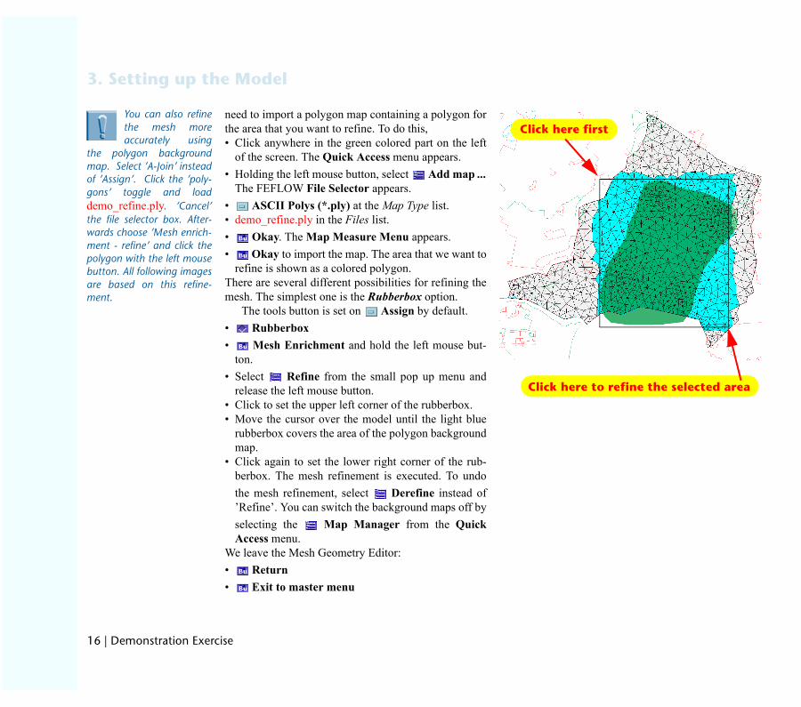
need to import a polygon map containing a polygon forthe area that you want to refine. To do this,• Click anywhere in the green colored part on the left

of the screen. The Quick Access menu appears. • Holding the left mouse button, select Add map ...

The FEFLOW File Selector appears.• ASCII Polys (*.ply) at the Map Type list. • demo_refine.ply in the Files list.• Okay. The Map Measure Menu appears.• Okay to import the map. The area that we want to

refine is shown as a colored polygon.There are several different possibilities for refining themesh. The simplest one is the Rubberbox option.

The tools button is set on Assign by default. • Rubberbox • Mesh Enrichment and hold the left mouse but-

ton.• Select Refine from the small pop up menu and

release the left mouse button. • Click to set the upper left corner of the rubberbox. • Move the cursor over the model until the light blue

rubberbox covers the area of the polygon backgroundmap.

• Click again to set the lower right corner of the rub-berbox. The mesh refinement is executed. To undothe mesh refinement, select Derefine instead of’Refine’. You can switch the background maps off byselecting the Map Manager from the QuickAccess menu.

We leave the Mesh Geometry Editor:• Return• Exit to master menu

ÅáëÉ

`äáÅâ=ÜÉêÉ=Ñáêëí

`äáÅâ=ÜÉêÉ=íç=êÉÑáåÉ=íÜÉ=ëÉäÉÅíÉÇ=~êÉ~

vçì=Å~å=~äëç= êÉÑáåÉíÜÉ= ãÉëÜ= ãçêÉ~ÅÅìê~íÉäó= ìëáåÖ

íÜÉ= éçäóÖçå= Ä~ÅâÖêçìåÇã~éK==pÉäÉÅí=Û^JgçáåÛ=áåëíÉ~ÇçÑ=Û^ëëáÖåÛK==`äáÅâ=íÜÉ=ÛéçäóJÖçåëÛ= íçÖÖäÉ= ~åÇ= äç~Çdemo_refine.plyK= Û`~åÅÉäÛíÜÉ= ÑáäÉ= ëÉäÉÅíçê= ÄçñK= ^ÑíÉêJï~êÇë=ÅÜççëÉ=ÛjÉëÜ=ÉåêáÅÜJãÉåí=J=êÉÑáåÉÛ=~åÇ=ÅäáÅâ= íÜÉéçäóÖçå=ïáíÜ=íÜÉ=äÉÑí=ãçìëÉÄìííçåK=^ää=ÑçääçïáåÖ=áã~ÖÉë~êÉ= Ä~ëÉÇ= çå= íÜáë= êÉÑáåÉJãÉåíK

PKO=qÜÉ=PêÇ=aáãÉåëáçå

PKO =qÜÉ=PêÇ=aáãÉåëáçå

Up to this point you have designed the geometry of atwo-dimensional model. The following steps describehow to introduce the third dimension into your modelusing FEFLOW. A three-dimensional finite elementmodel consists of a number of nodal planes, calledslices. These slices can generally be regarded as the topor bottom planes of the (geological) layers.

PKOKN aÉëáÖåáåÖ=päáÅÉë=~åÇ=i~óÉêë

• Dimension.

• Three-dimensional (3D) - The 3D Layer Config-urator pops up. See figure below.

The 3D-Layer Configurator controls the basic settingsfor the 3D model: • the number of layers and slices, • the data inheritance between slices or layers and • the relative position between the slices. The assignment of the real z coordinates is done later inthe 3D slice elevation editor.

You will now define the number of layers/slices youneed for this model. Of course the number may bechanged afterwards, if necessary.

dÑçÄÅ

ÄáíÇíëÄ~ëÉã

tÜÉå=ãçÇÉäáåÖ=çåÉä~óÉê= óçì= åÉÉÇ= íïçëäáÅÉëI= íÜÉ= íçé= ~åÇ

çííçã=ëäáÅÉK= =tÜÉå=ãçÇÉäJåÖ= íïç= ä~óÉêë= óçì= åÉÉÇÜêÉÉ=ëäáÅÉëI=íÜÉ=íçé=ëäáÅÉI=íÜÉáîáÇáåÖ= ëäáÅÉ= ÄÉíïÉÉå= íÜÉïç= ä~óÉêë= ~åÇ= íÜÉ= ÄçííçãäáÅÉK= = fåáíá~ä= ÅçåÇáíáçåë= ~åÇçìåÇ~êó= ÅçåÇáíáçåë= ~êÉëëáÖåÉÇ= íç= íÜÉ= åçÇÉë= çåäáÅÉëI=ïÜáäÉ=ã~íÉêá~ä=é~ê~ãJíÉêë= ~êÉ= ~ëëáÖåÉÇ= íç= ÉäÉJÉåíë=áå=ä~óÉêëK

fÑ= óçì=Ü~îÉ= ëâáééÉÇíÜÉ= éêÉîáçìë= ëíÉéëIéäÉ~ëÉ= äç~Ç= íÜÉ= ÑáäÉ

emo_2d.fem= îá~= íÜÉ=iç~ÇáåáíÉ= ÉäÉãÉåí= éêçÄäÉãéíáçå= Ñêçã= íÜÉ= cáäÉ= ãÉåìÉÑçêÉ= ÄÉÖáååáåÖ= íÜáë= ÉñÉêJáëÉK

cbcilt=ö=NT

NU=ö=aÉãçåëíê~íáçå=bñÉê


In our case the upper aquifer is limited by the groundsurface and by an aquitard at the bottom. The secondaquifer is situated below the aquitard, underlain by aclay layer of unknown vertical extension. We will cre-ate the slices necessary for the stratigraphy of the exist-ing area first:

In the Reference data box, enter an • elevation for the top slice at 1000 m in the Ele-

vation field and a • decrement of 100 m in the Decrement field. This will set the top slice of the model at an elevationof 1000 m, with all remaining slices set with a verticaldistance of 100 m apart. These settings will preventslices from intersecting when assigning real z-eleva-tions from borehole data.

We will now specify the 3D layers. • In the Number of layers input box, insert a value of

3. • Press Return to add the layers. The number of slices

automatically changes to 4 slices.As you can see, the 3D-Layer Configurator offersmany other tools, some of which we will need later inthis exercise. The online Help supplies you with moredetailed information about the functionalities. • Okay to exit the menu.

ÅáëÉ

PKP=mêçÄäÉã=`ä~ëë

PKP mêçÄäÉã=`ä~ëë

To define the parameters of the model we enter theProblem Editor Menu. All existing parameters areset to default values. We will only modify the mostimportant of these parameters. To enter the ProblemEditor,• Edit• Edit problem attributes ... - the Problem Edi-

tor appears.According to the FEFLOW philosophy, the most effi-cient procedure to build a model is to work from theuppermost menu entry down to the lower ones.

In the Problem Class window we will define theprincipal type of the FEFLOW model. For our pur-poses we need transient flow with mass transport for anunconfined aquifer using the BASD moving-grid tech-nique. For information about BASD click on the Helpbutton in the Free surface editor and follow the link tothe Theory section.• Problem class to enter the Problem Classifier.Since we are conducting a transient flow/transient masstransport model, perform the following settings:• Flow and Mass Transport.• Transient flow/transient transport• Unconfined (phreatic) aquifer(s).• Edit free surface(s) - The Free surfaces editor

appears. This will allow us to define the hydrogeo-logic properties of the slices.

• Set movable free surface on top - Now the topslice will follow the groundwater surface..

• Set unspecified where possible - These sliceswill be distributed according to the moving ground-water surface and the stratigraphy

• . Apply• Okay to exit the Problem Classifier.The model now describes an unconfined flow & masstransport problem with moving grid properties, i.e themesh will follow the moving groundwater table avoid-ing that mesh elements get partially saturated or evendry.

dÑçÄÅ

=fÑ=óçì=Ü~îÉ=ëâáééÉÇíÜÉ= éêÉîáçìë= ëíÉéëIéäÉ~ëÉ= äç~Ç= íÜÉ= ÑáäÉ

emo_3d.fem= îá~= íÜÉ= iç~ÇáåáíÉ= ÉäÉãÉåí= éêçÄäÉãéíáçå= Ñêçã= íÜÉ= cáäÉ= ãÉåìÉÑçêÉ= ÄÉÖáååáåÖ= íÜáë= ÉñÉêJáëÉK

cbcilt=ö=NV

OM=ö=aÉãçåëíê~íáçå=bñÉê


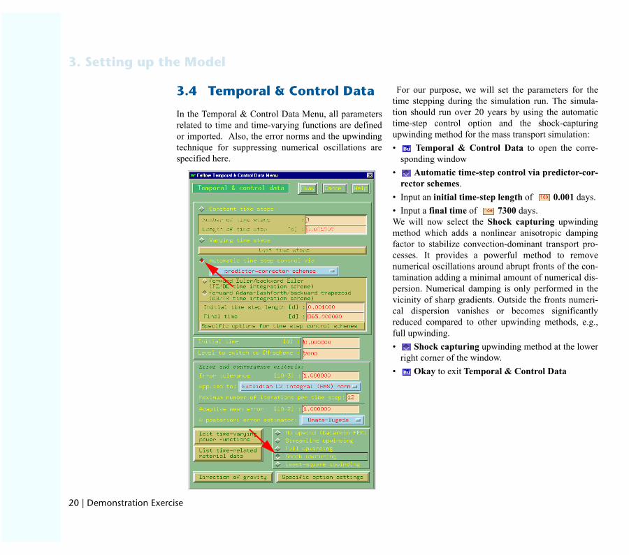
PKQ qÉãéçê~ä=C=`çåíêçä=a~í~

In the Temporal & Control Data Menu, all parametersrelated to time and time-varying functions are definedor imported. Also, the error norms and the upwindingtechnique for suppressing numerical oscillations arespecified here.

ÅáëÉ

For our purpose, we will set the parameters for thetime stepping during the simulation run. The simula-tion should run over 20 years by using the automatictime-step control option and the shock-capturingupwinding method for the mass transport simulation:• Temporal & Control Data to open the corre-

sponding window• Automatic time-step control via predictor-cor-

rector schemes. • Input an initial time-step length of 0.001 days. • Input a final time of 7300 days.We will now select the Shock capturing upwindingmethod which adds a nonlinear anisotropic dampingfactor to stabilize convection-dominant transport pro-cesses. It provides a powerful method to removenumerical oscillations around abrupt fronts of the con-tamination adding a minimal amount of numerical dis-persion. Numerical damping is only performed in thevicinity of sharp gradients. Outside the fronts numeri-cal dispersion vanishes or becomes significantlyreduced compared to other upwinding methods, e.g.,full upwinding.• Shock capturing upwinding method at the lower

right corner of the window.• Okay to exit Temporal & Control Data

PKR=PaJpäáÅÉ=bäÉî~íáçå

PKR PaJpäáÅÉ=bäÉî~íáçå

The 3D-Slice Elevation Menu allows you to define theslices based on real-world z-elevations by regionaliza-tion of irregularly distributed data points, i.e., fromborehole logging. Database regionalization of all initialvalues, boundary conditions and material parameterscan be assigned on the model as described for the z-ele-vations of the slices. • 3D- Slice elevation to enter the Slice Elevations

Menu.In the Layer configurator we had set the top slice to1000 m and the lower slices with a vertical spacing of100 m each. Now we will “pull down” the slices totheir real-world elevations by assigning the corre-sponding z-elevations. To avoid intersection we beginat the lowest slice:

• Select slice 4 by clicking on the corresponding num-ber in the Layers & Slices browser at the lower leftside of the screen. In the browser, the left columnlists the numbers of layers while the right columnlists the number of slices.

• As the database for the z-elevations is georeferencedin global cartesian coordinates, we have to make surethe global system is set. Click the coordinates box inthe lower left corner of the screen and choose „Global cartesian“.

• To import z-elevations for a slice based on boreholedata, we have to enter the Database RegionalizationMenu.

• Database option (at the right side of the meshinspector).

• z-Coordinates - An alert box pops up asking ifyou want to overwrite the existing values.

• Yes In the Data Regionalization Menu different interpola-tion methods for sample data are offered.

• Akima inter/extrapolation• Linear• In the neighboring points field, type 3. Only the

nearest three neighboring data points will be used forthe interpolation.

cbcilt=ö=ON

OO=ö=aÉãçåëíê~íáçå=bñÉê


• In the Acceptable over/undershooting field, type 0. This assures that the interpolation will be executedwithout smoothing the resulting surface.

• Import time-constant data - The file selectorappears and allows you to select the database for theinterpolation

• Choose bot_san2.trp from the Files list. This ASCIIfile (so called ’triplets file’) has an x-coordinate, y-coordinate, function-value format.

• Okay• Start in the Database Regionalization Window

and FEFLOW creates contours for slice 4, the bottomof layer 3 (see figure on the next page).

• Exit the Assign database function by clicking theright mouse button in the working window.

ÅáëÉ

• Browse to the next upper slice using the Layers &Slices browser and repeat the steps above to assignthe elevation data according to the list below.

You can display the resulting model domain in a 3Dview:• 3D-Options on the lower left side of the screen,

hold the mouse button. A small menu pops up• Visualize - A second menu pops up.• Body, release the mouse button. The Tricycler

window pops up and the model is displayed in 3-dimensional view (see figure).

• Move, rotate and zoom the model as described in themessage bar below the working window.

• Exiting rotation in the Tricycler window • Return to exit the 3D slice elevation menu

ëäáÅÉ Ç~í~Ä~ëÉ

4 (bottom of lower aquifer) bot_san2.trp3 (top of lower aquifer/bottom of aquitard)

bot_clay.trp

2 (top of aquitard/bottom of upper aquifer)

bot_san1.trp

1 (relief) demo_relief.trp

PKS=cäçï=a~í~

PKS cäçï=a~í~

The Flow Data section controls all the necessary inputparameters for the groundwater flow model. The Flowdata menu consists of three submenus: the Flow ini-tials, the Flow boundaries and the Flow materialsmenus. Click on the corresponding buttons to enter thesubmenus.• Flow Data to enter the first level of the Flow

Data Menu

PKSKN cäçï=fåáíá~äë

The Flow initials menu allows you to assign thegroundwater surface at the beginning of the transientsimulation run.• Flow initials• Database to import previously prepared point

data • Hydraulic head - The Database regionalization

window pops up.

cbcilt=ö=OP

OQ=ö=aÉãçåëíê~íáçå=bñÉê


In the Methods of regionalization, we select the Akimainterpolation technique again.• Akima inter/extrapolation• Switch to Linear.• In the neighboring points field, type 3.• In the Acceptable over/undershooting field, type

0.

ÅáëÉ

• Import database - The file selector appears. • Choose demo_head_ini.trp from the Files list. • Okay• Start - The regionalization will execute the inter-

polation of the data just imported (see resulting con-tours in the figure below).

• Exit the function by clicking the right mouse buttonin the model domain.

PKS=cäçï=a~í~

You can visualize the results.• Switch from Assign to Show.• Hydraulic head - FEFLOW shows the hydraulic

head distribution as colored fringes.• Switch from Show to Vanish.• Hydraulic head - FEFLOW resets to normal

view.We will now copy the initial values from slice 1 to allthe remaining slices.

Go to the Mesh Inspector icon and switch the lightblue Tools button to Copy..

• Hydraulic head - The Data Copier appears.• to ALL remaining slices• Start - You will be asked by an alert box if you

really want to overwrite the current values.• Yes• Return to close the Data Copier• Return to exit the Flow Initials Menu.

PKSKO cäçï=_çìåÇ~êáÉë

We should enter the Flow boundaries menu now andset the boundary conditions for our model. The picturebelow shows all parts of the menu.

We set the northern boundary condition first, whichdescribes the northern hills. In this exercise, for thesake of simplicity, we will assume a reasonable hydrau-lic potential along this border. Therefore we will set aconstant hydraulic head of 46 m. • Assign • Border• Head (1st kind)

jÉëÜ=áåëéÉÅíçê

=qççäë=çéíáçåë

hÉóÄç~êÇ=êÉèìÉëí=Äçñ

_çìåÇ~êó=ÅçåÇáíáçåë

=qççäë=

cbcilt=ö=OR

OS=ö=aÉãçåëíê~íáçå=bñÉê


• To be able to writethe value into theKeyboard requestbox, click into the box or hit the <TAB key>. Type

46 in the Keyboard Request box and hit theReturn key.

Move the cursor to the working window. Click the leftmouse button over the northeastern corner of the model

ÅáëÉ

domain and hold the button pressed. Move the cursor alittle bit to the northwest along the boundary andrelease the mouse button. Move on along the borderand click the last node in the northwest with the leftmouse button. Notice that all nodes in between havebeen assigned a head value of 46 m. The head bound-ary condition is indicated by blue circles.

båÇáåÖ=mçáåí

pí~êíáåÖ=mçáåí

eÉ~Ç=_çìåÇ~êó

åçêíÜÉêå=Üáääë

ä~âÉ=jΩÖÖÉäëÉÉ

fÑ=óçì=Ü~îÉ=~ëëáÖåÉÇíçç= ã~åó= åçÇÉëIëáãéäó= ëÉäÉÅí= íÜÉ

“kçÇ~ä“= çéíáçå= áå= íÜÉ“^ëëáÖå“= íççäI= ÅäáÅâ= çå= íÜÉ“eóÇê~ìäáÅ= eÉ~Ç“= ÄìííçåIÖç= íç= íÜÉ= ÜÉ~Ç= ÄçìåÇ~êóÅçåÇáíáçåë= óçì= ï~åí= íçÇÉäÉíÉ= ~åÇ= ÅäáÅâ= çå= É~ÅÜìåï~åíÉÇ= åçÇÉK= `äáÅâ= íÜÉêáÖÜí=ãçìëÉ=Äìííçå=íç=ÉñáíK

PKS=cäçï=a~í~

Now define the southern boundary conditions describ-ing the shoreline of Lake Müggelsee and the riverMüggelspree. We recommend to use the Assign -

border tool as described previously for the north-ern boundary. Set a Head boundary condition witha hydraulic head of 32.1 meters.

Afterwards switch the light blue Tools button toCopy.

• Head (1st kind) - The Data Copier appears.• to ALL remaining slices• Start - You will be asked by an alert box if you

really want to overwrite the current values.• Yes• Click Return to close the Copier menu.

The western and eastern borders of the model have notbeen assigned any values so far. Usually the riverswould be described by the third kind boundary condi-tion, Transfer. For this exercise let us assume theboundaries to be impervious. That means, we do nothave to prescribe any boundary condition at these bor-ders.

Once you have assigned the head boundary condi-tions for the northern and southern borders of ourmodel, assign the wells with their specific extractionrate. • Switch to the Join tool.• Supermesh • Load below the Supermesh option. The file

selector appears. •The selected supermesh will act as a frame for thefinite element mesh. It contains the polygon describingthe outer boundaries of the model and the Add-ins for

the exact positioning of the pumping wells and the con-taminant sources (waste disposal site, sewage treatmentplant).• Choose demo.smh in the Files list.• Okay• Now the imported supermesh including the Add-ins

is displayed in the working window.

The wells (boundary condi-tions) should be set on thesouthern part of the modelwhere the two Add-inpoints are positioned. For amore accurate setting of thewells, you can zoom intothis area using the zoomericons found among theinformation boxes.

We will now set the wells as boundary conditions of4th kind with a time-constant discharge rate. The pro-cedure is the same as before: • Join• Well (4th kind)• type a value of 1.000 m³/d into the Keyboard

request box• Move the cursor over one of the Add-ins. The under-

lying mesh node should be highlighted by a redsquare.

• Click the left mouse button to set the boundary con-dition with the defined discharge rate exactly on theAdd-in.

• Repeat this step for the second Add-in.• Once completed, click the right mouse button to exit

this function.

Zoom Pan

Back to last

Defaultextent

extent

cbcilt=ö=OT

OU=ö=aÉãçåëíê~íáçå=bñÉê


• We will now assign a value of zero (0) to the wells onall other slices. That causes the discharge rate speci-fied on the first slice to be distributed automaticallyon the different slices.

• Select the nextslice in the Layers& Slices browserlocated below theZoom option byclicking on theSlices number.

• Repeat the previous steps for each slice using a valueof 0 for the wells.

• Click Return to exit the Flow boundaries menu.

eÉ~ÇI=QS=ã

tÉääI=NMMMM=ã³LÇ

eÉ~ÇI=POKN=ã

ÅáëÉ

PKSKP cäçï=j~íÉêá~äë

The Flow Materials Menu allows you to edit all mate-rial parameters which have to be set for modeling agroundwater flow problem. • Flow materialsThe menu structure is similar to the Flow Boundariesmenu.

Upper AquiferThe conductivity of the upper aquifer will be importedfrom borehole samples stored in an ASCII database(syntax: X-coordinate, Y-coordinate, Conductivity).The method used is similar to the assignment of z-ele-vations in the 3D Slice elevation menu.• Ensure that the Assign tool is set.• Database• Conductivity [Kxx] - The Database regionaliza-

tion Window appears.• Akima inter/extrapolation• Set the number of neighbors to 3 and the over/

undershooting to 0 %.• Import time-constant data• Choose conduc2d.trp from the "Files" list.• Okay• Start in the Data Regionalization window.FEFLOW will now inter/extrapolate from the boreholedata and will display the resulting distribution as a con-tour map of conductivities (see figure to the right). Thecontours of our example show low conductivities nearthe northern hills and a high conductivity flow channelgoing down from the north to the south dividing themodel domain into two equal halfs.• Click the right mouse button after the interpolation is

finished.

PKS=cäçï=a~í~

You can visualize the results of the interpolation as col-ored fringes.• Show• Conductivity Kxx - The value distribution is dis-

played.• Vanish• Conductivity Kxx - FEFLOW resets to normal

view.We will now specify the storativity (drainable porosity)for the layer. • Assign• Global - This will assign the same value to the

entire layer.• Storativity (drain/fillable) - Here you assign the

drain/fillable porosity.

ä~âÉ=jΩÖÖÉäëÉÉ

åçêíÜÉêå=Üáääë
• An alert box pops up asking if you are sure to over-
write the data. Select Yes.• Input a value of 0.1 in the Keyboard request box

and press the Return key.• Exit the function by clicking the right mouse button.

AquitardOur next step is to prescribe the material properities ofthe Aquitard. Select Layer 2 in the Layers & Slicesbrowser.• Assign• Global• Conductivity [Kxx] - Again an alert box pops

up asking if you really want to overwrite the currentvalues.

• Yes• Input a value of 1e-6 in the Keyboard request

box corresponding to the unit 1e-4 m/s and press theReturn key.

• Exit the function by clicking the right mouse button.We will assign a new storativity value due to the lowconductivity we have set.• Assign• Global • Storativity (drain/fillable)• Yes• 0.01, press Return.• Quit the function by clicking the right mouse button.

Bottom AquiferTo the bottom aquifer we set a constant conductivity of10-3 m/s. • Layers: 3 in the Layers & Slices browser • Assign• Global

cbcilt=ö=OV

PM=ö=aÉãçåëíê~íáçå=bñÉê


• Conductivity [Kxx]• Yes• 10, press Return.• Exit the function by clicking the right mouse button.Now we copy the K[xx] values to the K[yy] and K[zz]parameter to create isotropic conductivities in all lay-ers. • Copy• Conductivity Kxx - The FEFLOW Data

Copier appears.

• Switch the light blue button from Layer-Relatedto Advanced

• Ensure that the Copy to Kyy-Conductivity and Copy to Kzz-Conductivity toggles are selected

in the upper part of the menu• at all layers • Start

ÅáëÉ

• You will be asked twice by an alert box if you reallywant to overwrite the current values.

• Select Yes both times.

• Return to close the Data Copier

Groundwater RechargeThe assignment of the groundwater recharge will beexecuted using a template showing the areas of differ-ent landuses and an ASCII database containing theattribute data. The polygon file is linked with the data-base.

• Layers: 1 in the Layers & Slices browser• Join• Polygon• Load below the "Polygon" option. The File

Selector pops up. • Choose recharge_normal_year.ply in the Files list.

PKS=cäçï=a~í~

• Okay to leave the file selector.Now the Parameter Association window becomesvisible.

On the left hand side the field names of the databaseare listed. On the right hand side the FEFLOW parame-ters are shown. Two pipelines connect the right handlist with the left hand side. The polygon IDs are linkedwith the field “ID” of the database. The data of the“MEAN” field is linked to the FEFLOW parameter“In/outflow on top/bottom”.

You can add and remove links. However, for thisdemo exercise just click• Okay

•

• The polygon file is displayed as template in theworking window

• In(+)/out(-) flow on top - An alert box appearstelling you the different database link options (seenext page).

• Overlay in the alert box. The database valueswill automatically be assigned to the model. Fordetailed information about this database link see theFEFLOW online help.

• click the right mouse button.Now leave the Flow materials and Flow data menus byhitting Return two times.

You have created an executable transient flowproblem now. Changing the problem class to "flowonly" and eventually to „steady flow“ allows you tomake a first trial on the simulation and to skip the nextsections regarding the transport parameter settings.

íóÄbå

=qÜÉ=äáåâë=Ü~îÉ=ÄÉÉåëÉí= ÄÉÑçêÉ= ÇìêáåÖíÜÉ= éêÉé~ê~íáçå= çÑ

ÜÉ= ÉñÉêÅáëÉ= Ç~í~K= cçê= ìëáåÖçìê=çïå=Ç~í~=íÜÉó=Ü~îÉ=íçÉ= ëÉí= ã~åì~ääóK= fÑ= ìëáåÖpof=ëÜ~éÉ=ÑáäÉëI=íÜÉ=fa=äáåâ=áëçí=åÉÅÉëë~êó>

fÑ= cbcilt= ÇçÉëåçí= Çáëéä~ó= íÜÉ~äÉêí= ÄçñI= éäÉ~ëÉ

ÅÜÉÅâ= óçìê= ÑáäÉ= ~ÅÅÉëë= éÉêJãáëëáçåëK= têáíáåÖ= éÉêãáëJëáçå=áå=íÜÉ=t^pvLcbciltLÉñÉêÅáëÉLáãéçêíHÉñéçêíLÇáêÉÅíçêó=áë=åÉÅÉëë~êó>

cbcilt=ö=PN

PO=ö=aÉãçåëíê~íáçå=bñÉê


ÅáëÉ

PKT qê~åëéçêí=a~í~

Enter the Transport Data menu from the ProblemEditor. This menu contains all editors for defining massand heat transport parameters. Its structure is similar tothe Flow Data menu, i.e., you can set initial values,boundary conditions and material parameters.

The Mass transport initials, which describe theinitial concentration of the model, remain on thedefault value of 0 mg/l.

PKTKN j~ëë=qê~åëéçêí=_çìåÇ~êáÉë

In the Mass transport boundaries menu, "freshwater" conditions - at very low concentrations - will beassigned to the outer borders where water can enter themodel. The contaminant sources are situated on the topslice.

Click on Mass transport boundaries to enterthe menu.• Switch to the Assign tool .

PKT=qê~åëéçêí=a~í~

• Border • Mass (1st kind)• Type the value of 1e-12 mg/l into the Keyboard

request box.• Move the cursor in the working window to the north

eastern corner of the model.• Click and hold the left mouse button on the first node

at the northeastern border. Move the cursor along themodel boundary still holding the left mouse button.Free the left mouse button. All border nodes youhave passed should be marked by a blue circle. Goon until you reach the last node at the northwesternedge. Click the node with the left mouse button.

• Repeat the same procedure for the southern border.• Exit the function clicking the right mouse button in

the working window.The model boundary is now set for freshwater condi-tions. These fresh water conditions have the disadvan-tage that outflowing water is set to this concentration,too, if passing the border. A contaminant plume cannotleave the model freely. Therefore we will limit theactivity of the fresh water conditions by so-called Con-straints. This guarantees that the first-kind boundarycondition of fresh water is only set when water entersthe model (inflow). On the other hand, if an outflowsituation occurs at such a constrained boundary, thefirst-kind boundary condition of fresh water is auto-matically switched off and the contaminant mass canfreely outflow (if boundary is open for convection). Fordetailed information see the Reference Manual. Weassign for northern and southern borders a complemen-tary minimum constraint of 0 m³/d mg/l.

Click on the arrow-sign right of the Mass (1stkind) button. The corresponding Constraint Condi-tions menu becomes visible.

Input the Min-constraint of 0 mg/l m³/d in the firstrow.

Click on the Min toggle left of the input fieldfor activating the setting.

Click on Mass (1st kind).Assign the constraint along the northern and south-

ern border. As the border option is not available herekeep the left mouse button pressed and try to move themouse over all border nodes.

Leave the Constraints menu via the arrow-signed button.

Next we will assign the boundary conditions for thetwo contamination sources, the sewage water treatmentplant and the waste disposal site, which are placed inthe northern part of the model.• Join• Supermesh • Load below the Supermesh option. The file

selector pops up.• Choose demo.smh from the Files list • Okay button. Now the supermesh including the

Add-ins is displayed.• Mass (1st kind) • Enter a value of 500 mg/l in the Keyboard

request box in order to represent contaminant release

`çåëíê~áåí= ~åÇ_çìåÇ~êó= `çåÇáJíáçåë= ~êÉ= Ü~åÇäÉÇÇáÑÑÉêÉåíäó= Ñçê

ÑäìñÉëW= = cçê= `çåëíê~áåí`çåÇáíáçåë=fåÑäçïë=~êÉ=éçëJáíáîÉ=EHFI=lìíÑäçïë=~êÉ=åÉÖJ~íáîÉ= EJFK= cçê= _çìåÇ~êó`çåÇáíáçåë= fåÑäçïë= ~êÉåÉÖ~íáîÉ= EJFI= lìíÑäçïë= ~êÉéçëáíáîÉ=EHFK

cbcilt=ö=PP

PQ=ö=aÉãçåëíê~íáçå=bñÉê


at the sewage treatment plant to the west and thewaste disposal site to the east.

• Press the Return key.• First, move the mouse to the sewage facility (west

side) directly over the Add-in line. Notice that theline becomes highlighted.

• Click the left mouse button to assign the contaminantconcentration.

• Repeat the step for the waste disposal facility (eastside).

• Click the right mouse button to exit the function.We will now copy these boundary conditions to allremaining slices.• Copy• Mass (1st kind) - The Data Copier appears.

ÅáëÉ

• Notice the possibility to copy boundary conditionswith or without the related constraint conditions.Choose the option Boundary conditions withrelated constraints if exist.

• to ALL remaining slices• Start• A FEFLOW alert box pops up. Select Yes to

overwrite the values.• Return" to exit the Data Copier.

We will now leave the Boundaries menu and enter theMass transport materials menu.• Return• Mass transport materials

PKT=qê~åëéçêí=a~í~

PKTKO j~ëë=qê~åëéçêí=j~íÉêá~äë

All material parameters concerning mass transport areset in the Mass Transport Materials Menu. We will firstassign the values for the total porosity of the aquifer forthe top layer:• Assign• Global • Porosity• A FEFLOW alert box appears. Select Yes to

overwrite the default value globally.• Input a value of 0.2 in the Keyboard request box.• Press the Return key and leave the function hitting

the right mouse button.

As the next step we specify the contaminant masstransport dispersivity for our model. • Assign• Global • Longitudinal dispersivity• Yes• Input a longitudinal dispersivity value of 70 m in

the Keyboard request box.• Press the Return key and leave the function hitting

the right mouse button.• Repeat the steps for Transverse dispersivity,

assigning a value of 2.5 m• Copy the dispersivity values to all layers using the

Copy tool.• Exit the Transport data menu by selecting

Return and go up to the Problem Editor Menu.

łmçêçëáíó“= ~ë= ~ã~ëë= íê~åëéçêíã~íÉêá~ä= éêçéÉêíó

ãÉ~åë=íÜÉ=íçí~ä=éçêçëáíó=áåÅçåíê~ëí= íç= íÜÉ= łëíçê~íáîJáíó“= î~äìÉ= çÑ= íÜÉ= Ñäçïã~íÉêá~äëI=ïÜáÅÜ=çåäó=í~âÉëáåíç=~ÅÅçìåí=íÜÉ=Çê~áå~ÄäÉéçêçëáíóK

cbcilt=ö=PR

PS=ö=aÉãçåëíê~íáçå=bñÉê


PKU oÉÑÉêÉåÅÉ=a~í~

At last you should set some observation points to thetop slice. For the points, all resulting data such ashydraulic heads or contaminant concentrations arevisualized online in diagrams during the simulationrun.• Reference data• Observation single points

ÅáëÉ

• Import points - The file selector pops up. Nowyou will import the observation points from anASCII database.

• Choose demo_obs_pnts.pnt• OK - The points are loaded and visualized as col-

ored circles.• Leave the reference data editor for the Problem edi-

tor by clicking on the two Return buttons.

PKV=oÉÅçåÑáÖìêÉ=Pa=q~ëâ

PKV oÉÅçåÑáÖìêÉ=Pa=q~ëâ

The basic model parameters are now assigned, but wewill add two additional layers to increase the accuracyof modeling the aquitard. Therefore we have to re-enterthe Layer configurator via the 3D-Slice elevationsmenu.

• 3D-Slice elevation in the Problem Editor• Reconfigure 3D Task

• Type a decrement of 1000 m in the Decrementbox. This unrealistic high decrement makesFEFLOW divide the aquitard equally spaced in threenew layers.

• Change the Number of layers in the input box at theupper left corner of the menu to 5.

• Press Return.• The Slice Partitioner pops up• Partitioning according to the list • Move the cursor to the Partitioning list. • Scroll the Partioning list using the vertical slider bar

at the right of the menu and replace the 2 automati-cally set by FEFLOW beneath 4. slice fixed by 0.

• Between the 2. slice is fixed and 3. slice is fixedreplace the 0 by 2.

The z-elevations of the new slices are interpolated fromthe nodal values of the upper and lower slice. Thereforethe new slice will divide the aquitard evenly.• OK

cbcilt=ö=PT

PU=ö=aÉãçåëíê~íáçå=bñÉê


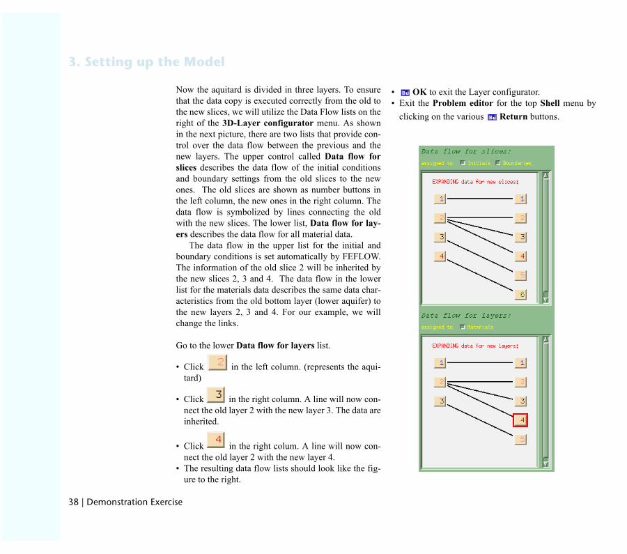
Now the aquitard is divided in three layers. To ensurethat the data copy is executed correctly from the old tothe new slices, we will utilize the Data Flow lists on theright of the 3D-Layer configurator menu. As shownin the next picture, there are two lists that provide con-trol over the data flow between the previous and thenew layers. The upper control called Data flow forslices describes the data flow of the initial conditionsand boundary settings from the old slices to the newones. The old slices are shown as number buttons inthe left column, the new ones in the right column. Thedata flow is symbolized by lines connecting the oldwith the new slices. The lower list, Data flow for lay-ers describes the data flow for all material data.

The data flow in the upper list for the initial andboundary conditions is set automatically by FEFLOW.The information of the old slice 2 will be inherited bythe new slices 2, 3 and 4. The data flow in the lowerlist for the materials data describes the same data char-acteristics from the old bottom layer (lower aquifer) tothe new layers 2, 3 and 4. For our example, we willchange the links.

Go to the lower Data flow for layers list.

• Click in the left column. (represents the aqui-tard)

• Click in the right column. A line will now con-nect the old layer 2 with the new layer 3. The data areinherited.

• Click in the right colum. A line will now con-nect the old layer 2 with the new layer 4.

• The resulting data flow lists should look like the fig-ure to the right.

ÅáëÉ

• OK to exit the Layer configurator.• Exit the Problem editor for the top Shell menu by

clicking on the various Return buttons.

Enter the simulator via the Simulator shell menuby selecting Run ...

Start the simulation by clicking on (Re-)Runsimulator. Notice that FEFLOW automatically gener-ates various windows that detail the ongoing results forthe wells, observation points, hydraulic head and con-taminant concentrations. These windows display theresults as diagrams. For the possibilities of editing thediagram properties please see the online help.

The transient simulation will require approximately10 minutes on a Pentium III 1.1 GHz. If you don’t wantto wait, we have already prepared a results file, whichyou can view in the Postprocessor Menu.

Having interrupted or completed the simulation,you can analyze the results of the current time step withthe options offered in the Halt & View Results menu(isoline maps, velocities, particle tracking, dataexport), the Budget analyzer, the Fluid flux analyzer orin the spatial operations window. The same possibili-ties are available in the Postprocessor, where analyzingis enabled for all of the saved time steps.

• Return to exit the Simulator.

Äë

íÅÅíÛíÛï

dîéãÉ

Q
qÜÉ=páãìä~íçê
In this step the simulation run is performed.

vçì= Å~å= ëíçé= íÜÉëáãìä~íáçå=Äó=éêÉëëJáåÖ= YbëÅ[K= oÉëí~êí

ó= ÅäáÅâáåÖ= çå= “EoÉJFoìåáãìä~íçêÒK

vçì= Å~å= éÉêÑçêã= ~ëíÉ~Çó= ÑäçïLëíÉ~Çóíê~åëéçêí= ëáãìä~J

áçå= íç= ë~îÉ= íáãÉK= få= íÜáë~ëÉ= ëïáíÅÜ= íÜÉ= ÛmêçÄäÉãä~ëëÛ=íç=ÛpíÉ~Çó=ÑäçïLëíÉ~Çóê~åëéçêíÛ= ~åÇ= ÅÜ~åÖÉ= íÜÉj~ñáãìã=åìãÄÉê=çÑ= áíÉê~Jáçåë= éÉê= íáãÉ= ëíÉéÛ= áå= íÜÉqÉãéçê~ä= C= Åçåíêçä= Ç~í~ÛáåÇçï=íç=ÛNRÛK

=fÑ=óçì=Ü~îÉ=ëâáééÉÇíÜÉ= éêÉîáçìë= ëíÉéëIéäÉ~ëÉ= äç~Ç= íÜÉ= ÑáäÉ

emo_transport_3d.femá~= íÜÉ= iç~Ç= ÑáåáíÉ= ÉäÉãÉåíêçÄäÉã=çéíáçå=Ñêçã=íÜÉ=cáäÉÉåì= ÄÉÑçêÉ= ÄÉÖáååáåÖ= íÜáëñÉêÅáëÉK

cbcilt=ö=PV

QM=ö=aÉãçåëíê~íáçå=bñÉê

QK=qÜÉ=páãìä~íçê

ÅáëÉ

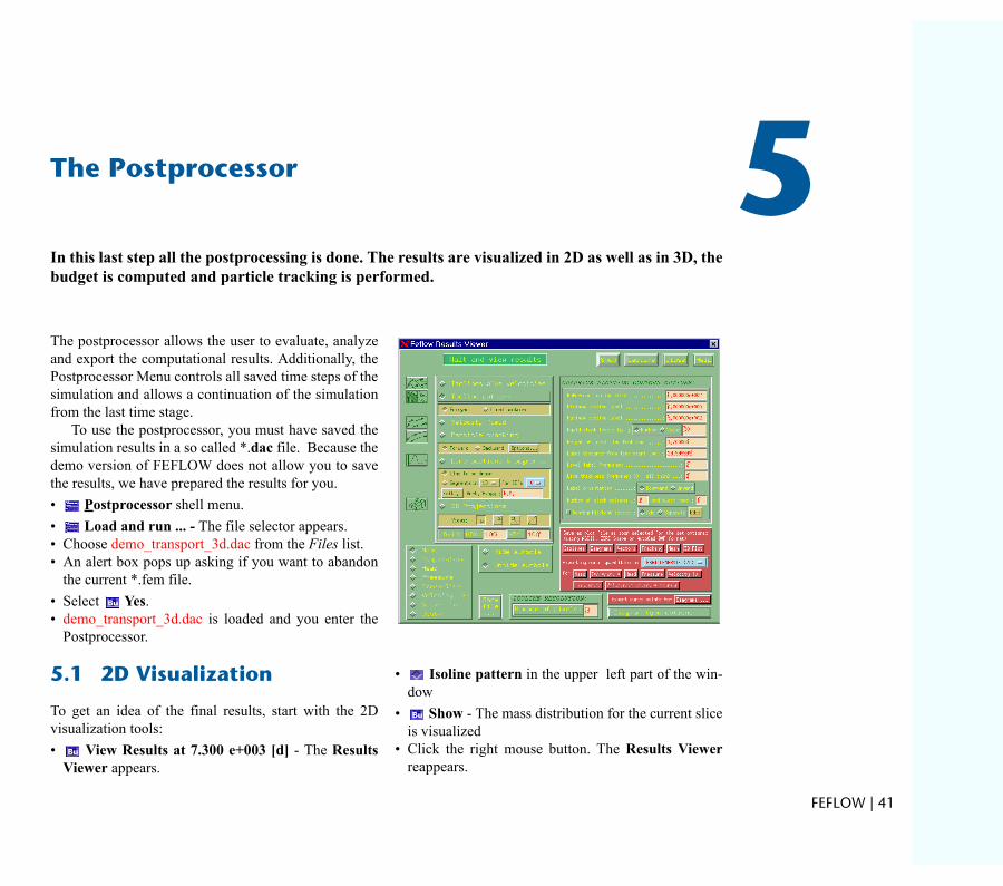
The postprocessor allows the user to evaluate, analyzeand export the computational results. Additionally, thePostprocessor Menu controls all saved time steps of thesimulation and allows a continuation of the simulationfrom the last time stage.

To use the postprocessor, you must have saved thesimulation results in a so called *.dac file. Because thedemo version of FEFLOW does not allow you to savethe results, we have prepared the results for you.• Postprocessor shell menu.• Load and run ... - The file selector appears. • Choose demo_transport_3d.dac from the Files list.• An alert box pops up asking if you want to abandon

the current *.fem file. • Select Yes.• demo_transport_3d.dac is loaded and you enter the

Postprocessor.

RKN Oa=sáëì~äáò~íáçå

To get an idea of the final results, start with the 2Dvisualization tools:• View Results at 7.300 e+003 [d] - The Results

Viewer appears.

• Isoline pattern in the upper left part of the win-dow

• Show - The mass distribution for the current sliceis visualized

• Click the right mouse button. The Results Viewerreappears.

R
qÜÉ=mçëíéêçÅÉëëçê
In this last step all the postprocessing is done. The results are visualized in 2D as well as in 3D, thebudget is computed and particle tracking is performed.

cbcilt=ö=QN

QO=ö=aÉãçåëíê~íáçå=bñÉê

RK=qÜÉ=mçëíéêçÅÉëëçê

Cross sections can be visualized for all parameter dis-tributions along lines. The lines can be drawn in theworking window or imported in ESRI generate format.First draw a cross section:

• Click Edit... below the Line sections & seg-ments entry and hold the mouse button.

• Draw segments • Now you have to draw the line for the cross sec-

tion(s) on the working window. Refer to the followfigure:

ÅáëÉ

• Click the start point for the cross section on themodel. Digitize the cross section by clicking on themodel.

• Click the right mouse button to end the editing of aline. The line gets an ID number.

• Click with the right mouse button a second time. TheResults Viewer reappears.

Now we will define an isoline contour for the hydraulichead along the cross section that also shows the veloci-ties at the nodes:

• Lined contours in the upper left part of the win-

dow.• Line sections & segments• Segments• 2D+. The + indicates additional visualization of

velocity vectors at the nodes.

RKN=Oa=sáëì~äáò~íáçå

• Head in the lower left part of

the window for analyzing thehydraulic head distribution.

• Show - A vertical cross sec-tion of the hydraulic head distri-bution is displayed.

• Click with the right mouse button. The ResultsViewer reappears.

We will now analyze the flow pathlines to the wellsusing the particle tracking option:• Switch to Slice 3 in the Layers & Slices browser at

the lower left side of the screen to start the pathlinesfrom this nodal plain.

• Particle tracking

• Backward• Options... - The Pathline editor appears.

• multiple pathlines around a single well in theleft row. This option allows you to start multiplepathlines exactly from a well to visualize capturezones.

• Close to leave the Pathline editor.

cbcilt=ö=QP

QQ=ö=aÉãçåëíê~íáçå=bñÉê


• Show to start the pathline function. The workingwindow displays the border of the model and sym-bols for the wells.

• Click on a well location to create the backward(reverse) particle tracking.

• Click with the right mouse button to exit the func-tion. The Results Viewer reappears.

At last try out the Pseudo 3D Visualization for parame-ter distributions:

• 3D Projections. • Mass in the lower left part of the menu.• Show - The mass distribution is visualized as a

3D plot, where the quantity of mass concentration isvisualized along the z axis.

• Click with the right mouse button to exit the func-tion. The Results Viewer reappears.

• Close to close the Results Viewer.

ÅáëÉ

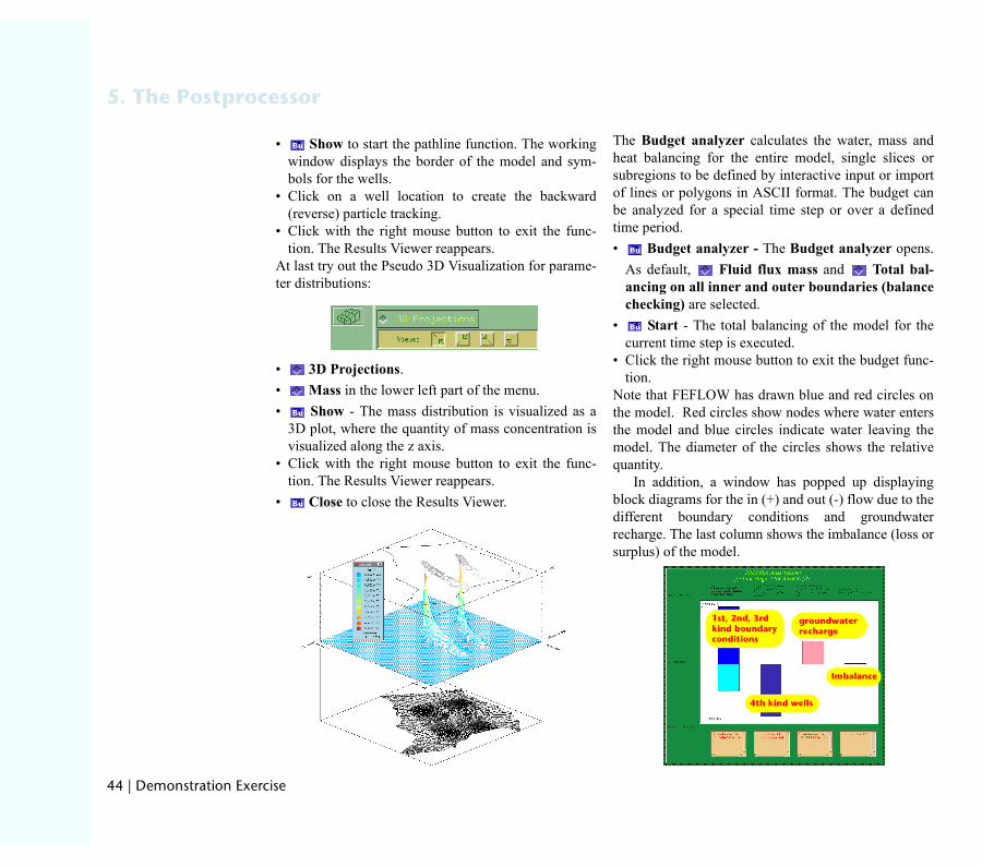
The Budget analyzer calculates the water, mass andheat balancing for the entire model, single slices orsubregions to be defined by interactive input or importof lines or polygons in ASCII format. The budget canbe analyzed for a special time step or over a definedtime period.• Budget analyzer - The Budget analyzer opens.

As default, Fluid flux mass and Total bal-ancing on all inner and outer boundaries (balancechecking) are selected.

• Start - The total balancing of the model for thecurrent time step is executed.

• Click the right mouse button to exit the budget func-tion.

Note that FEFLOW has drawn blue and red circles onthe model. Red circles show nodes where water entersthe model and blue circles indicate water leaving themodel. The diameter of the circles shows the relativequantity.

In addition, a window has popped up displayingblock diagrams for the in (+) and out (-) flow due to thedifferent boundary conditions and groundwaterrecharge. The last column shows the imbalance (loss orsurplus) of the model.

fãÄ~ä~åÅÉ

ÖêçìåÇï~íÉêêÉÅÜ~êÖÉ

QíÜ=âáåÇ=ïÉääë

NëíI=OåÇI=PêÇâáåÇ=ÄçìåÇ~êó=ÅçåÇáíáçåë

RKO=PaJléíáçåë=jÉåì

RKO PaJléíáçåë=jÉåì

For a detailed 3D description of our model, and toreview all parameters, we exit to the main menu.

You can enter the 3D options menu from either theShell menu, the Postprocessor or the Problem Editor.You enter the 3D Options menu via the green 3DOptions button at the lower left side of the screen,below the Layers & Slices browser.• Click 3D Options and hold the mouse button.• Visualize• Fringes• Materials• Kxx

The conductivity in the x-direction is visualized as a3D object. Additionally the Tricycler menu appears.• Click on the model, hold the left mouse button and

move the mouse in order to rotate the model.• Press the <Ctrl> key and move the mouse up and

down to zoom in or out. Click the middle mouse bot-ton to pan the model.

cbcilt=ö=QR

QS=ö=aÉãçåëíê~íáçå=bñÉê


RKOKN PaJm~íÜäáåÉ=^å~äóòÉê

One of the main 3D analyzing tools FEFLOW offers isthe 3D pathline visualization. You can start the path-lines by positioning the starting point via the 3D cursoron the model (move the red handlers), by starting themfrom a specified slice or by importing an ASCII file forthe computation of the Relevant Area of Influence(RAI) for a well. We will start now some pathlinesfrom the second slice.• 3D Options, hold the mouse button• Pathline - The 3D Pathline Controller is opened.

ÅáëÉ

• Start on 2D slice• Insert 2 in the Current slice field • Start new pathlines - The selected slice is visu-

alized. The cursor is in the zoom mode.• Click with the right mouse button to deactivate the

zoomer.• Click any number of arbitrary points in the northern

part of the model. Each point will be a starting pointfor a pathline.

• Click with the right mouse button. The visualizationis executed.

RKO=PaJléíáçåë=jÉåì

RKOKO PaJfëçëìêÑ~ÅÉë

The visualization of isosurfaces gives the predictedplume of the contaminant plume. Visualize now anIsosurface for mass concentration:• 3D Options, hold the mouse button• Visualize -The 3D Pathline Controller is opened.• Isosurfaces• Mass CA mean isosurface for the mass concentration is visual-

ized. For defining different isosurfaces just • click Properties in the Tricyler. The Properties

menu pops up.• click the General folder and insert the isosurface

value, e.g., 50 mg/l.• press the Return key. The isosurface is displayed. In the Components part of the Tricycler you canswitch the different isosurfaces on and off. To exit the3D Options menu, simply click on the Exitingrotation button located in the lower right corner of theTricycler menu.)

cbcilt=ö=QT

QU=ö=aÉãçåëíê~íáçå=bñÉê


RKP cáå~ä=oÉã~êâë

This completes the FEFLOW Demonstration Exercise.Please take some time to familiarize yourself with themany features offered by FEFLOW.

As a next step for getting introduced to FEFLOWwe recommend to go through the Tutorial, which youcan find in the second part of the User’s Manual.

For further questions please refer to the online Helpfound in all menus and windows by hitting <F1> orclicking the Help button.

For information on special topics please have a look atthe FEFLOW documentation, which you find on yourFEFLOW CD in the ’doc’ directory. If you are in pos-session of a FEFLOW license, you have gotten the doc-

ÅáëÉ

umentation in book-form, too. Pay attention to thefollowing documents in particular:• User’s manual (users_manual.pdf):

FEFLOW handling, tutorial for advanced users,introduction to the interface manager IFM

• Reference manual (reference_manual.pdf):all the theory behind FEFLOW

• White Papers Vol. I and II (white_papers_vol1.pdfand white_papers_vol2.pdf):papers on special topics (benchmarks, numericalmethods etc.)

Browse to http://www.feflow.info for up-to-date infor-mation concerning current releases, FAQs, etc.

If you wish to attend a training course on the app-plication of FEFLOW please contact your local distrib-utor or WASY for proposed dates and course programs.

t^pv pçÑíï~êÉ cbcilt = o - tu-braunschweig.de · t^pv=pçÑíï~êÉ cbcilt =...

Documents