tr 063 - tech.ebu.ch
TRANSCRIPT

TR 063
5G BROADCAST NETWORK
PLANNING AND EVALUATION
SOURCE: S-SPT
Geneva
August 2021

This page is intentionally left blank

TR 063 5G Broadcast Network Planning & Evaluation
3
Abstract
The way in which the content and services of Public Service Media (PSM) organizations are delivered
is evolving, particularly driven by the popularity of personal devices (smartphones, tablets) for
accessing audiovisual (AV) media.
Whilst PSM content and services can be accessed on smartphones and tablets, this is only under
conditions that do not comply with the fundamental requirements of PSM organizations. In particular,
the need to deliver linear services free to air to all audiences, everywhere and at any time. This
so-called universality principle lies at the core of the PSM remit.
Since the early 2000s, therefore, PSM organisations have tried to establish full access to such devices
by including a broadcast receiver within them. All these attempts, which used different broadcast
technologies – DVB-H, MediaFlo, ISDB-T Seg1, DVB-T2 Lite etc., have been unsuccessful.
The new technology called LTE-based 5G Terrestrial Broadcast (abbreviated to “5G Broadcast” in this
report), developed and specified as part of the general mobile communication technology of 3GPP,
is a broadcast mode of operation that seems to be a promising candidate for finally allowing all PSM
services, both linear and nonlinear, to reach smartphones and tablets.
Many PSM organizations around the world are considering 5G Broadcast. However, before adopting
this new technology it is crucial for PSM organisations to understand what the implications of such a
decision would be. This refers to the potential and pitfalls of this new audio-visual distribution option
in terms of technology, regulatory constraints and business implications. This report sheds some light
on the network planning of 5G Broadcast. The frequency planning of 5G Broadcast, including sharing
and compatibility between 5G Broadcast and other DTT systems in the spectrum range 470 – 694 MHz
is dealt with in a separate EBU Technical Report, TR 064.
Extensive studies have been carried out. Both theoretical (i.e. regular gridded) networks, and
real-world network topologies have been investigated, based on sets of scenarios and related
technical parameters (as described in this report and its Annexes). One aim of these studies is to
address whether broadcasting infrastructure, including High Power High Tower and Medium Power
Medium Tower could be employed to provide 5G Broadcast services to Car-Mounted and Handheld
Portable receivers.
Information on the status of 5G standardization, including 5G Broadcast, and deployment
opportunities can be found in EBU Technical Report TR 054 “5G for the Distribution of Audiovisual
Media content and services”.
The main findings of the studies carried out of this report can be summarised as follows:
1. All ‘Homogeneous’1 network topologies based on using only one type of site (HPHT, MPMT
or LPLT)2 have drawbacks when considered separately for 5G Broadcast coverage. HPHT
or MPMT alone offer good coverage for Fixed roof-top with low site density but do not
provide good coverage for Mobile reception in all environments. On the other hand, LPLT
1 Homogeneous means that only one type of site is used in the network. 2 HPHT: High Power High Tower networks
MPMT: Medium Power Medium Tower networks
LPLT: Low Power Low Tower networks
The characteristics of these networks are defined in Annex A.

5G Broadcast Network Planning & Evaluation TR 063
4
alone provides good coverage for Mobile (as well as for Handheld and Fixed) in all
environments but requires high site density.
2. Hybrid networks including three layers of HPHT, MPMT and LPLT offer the best compromise
between good coverage for mobile and reasonable site density. The word Hybrid here is
not a simple mixture of sites but true three-layer networks, with HPHT sites serving as
umbrella, complemented underneath by MPMT sites in some rural and suburban areas,
which are complemented underneath by LPLT sites in urban areas.
3. Such hybrid topologies can provide sufficiently high SINR levels (up to 15 dB) to allow the
use of efficient 5G Broadcast Modulation and Coding Schemes reaching throughputs of up
to 7 Mbit/s in 5 MHz, in Mobile and handheld reception conditions.
4. The use of the same frequency and the same editorial content in SFN mode between all
sites and layers offers the best performance, thanks to the gain offered by such networks.
However, Single Frequency Networks (SFNs) may not be implementable over very large
areas due to editorial content change across borders, and to the current interleaved use
of spectrum for DTT imposed by the Geneva 2006 Agreement (GE06). Therefore, a mixture
of MFN and SFN would be required, within the constraints of GE06. Future studies may
investigate closed SFNs3 using the same frequency across border areas to mitigate the need
for MFN.
5. Trials are needed to verify the conclusions and the assumptions of the studies. Future
studies should consider enhancement techniques for mobile reception, such as time
interleaving.
3 A Closed SFN uses directional antenna patterns at transmitters located at its edge, oriented towards the centre of the
SFN, to reduce the outgoing interference to neighbouring co-channel networks.

TR 063 5G Broadcast Network Planning & Evaluation
5
List of Acronyms and Abbreviations
The following terms are used throughout this report:
Abbreviation /
Acronym Expansion
3GPP 3rd Generation Partnership Project
BNO Broadcast Network Operator
BW Bandwidth
CAS Cell Acquisition Subframe
CDF Cumulative Distribution Function
CE Channel Estimation
C/I Carrier to interferer ratio
C/N Carrier to noise ratio
CM Car Mounted
CP Cyclic prefix (mobile term) - equivalent to Guard Interval (broadcast term)
DAB Digital Audio Broadcasting
DTM Digital Terrain Model
DTT Digital Terrestrial Television
DVB Digital Video Broadcasting
DVB-H Digital Video Broadcasting — Hand held
DVB-T Digital Video Broadcasting — First Generation Terrestrial
DVB-T2 Digital Video Broadcasting — Second Generation Terrestrial
EIRP Equivalent Isotropically Radiated Power
ERP Equivalent (or Effective) Radiated Power
eMBMS Evolved Multimedia Broadcast Multicast Services
FeMBMS Further Evolved Multimedia Broadcast Multicast Services
FFT Fast Fourier Transform
GE06 Geneva Agreement 2006
GI Guard Interval
HH Handheld
HPHT High-Power High-Tower
ICI Inter Carrier Interference
ISD Inter-Site Distance
ISDB-T 1 seg Integrated Services Digital Broadcasting -– Terrestrial for handheld mobile reception
ITU International Telecommunication Union
LPLT Low-Power Low-Tower
LTE Long Term Evolution
LTE-B / MediaFlo Qualcomm proprietary broadcast system aimed at handheld reception
MCS Modulation and Coding Scheme
MFN Multi Frequency Network
MNO Mobile Network Operator

5G Broadcast Network Planning & Evaluation TR 063
6
Abbreviation /
Acronym Expansion
MPMT Medium-Power Medium-Tower
OFDM Orthogonal Frequency-Division Multiplexing
PMCH Physical Multicast Channel
PO Portable Outdoor
PSM Public Service Media
QAM Quadrature Amplitude Modulation
QPSK Quadrature phase shift keying
RB Resource block
SFN Single Frequency Network
SINR Signal to Interference plus Noise Ratio
SNR Signal to Noise Ratio

TR 063 5G Broadcast Network Planning & Evaluation
7
Contents
Abstract ................................................................................................... 3
List of Acronyms and Abbreviations ................................................................. 5
1. Theoretical Network model and simulation results ..................................... 9
1.1 Introduction.............................................................................................................. 9
1.2 Network topologies and frequency reuse........................................................................... 9
1.3 Reception modes and parameters ................................................................................. 13
1.4 Simulation methodology ............................................................................................. 14
1.5 Coverage of national or regional border areas .................................................................. 18
1.5.1 Background ......................................................................................................... 18
1.5.2 Results ............................................................................................................... 19
1.5.3 Discussion ........................................................................................................... 20
1.5.4 Conclusion .......................................................................................................... 22
1.6 Results .................................................................................................................. 22
1.6.1 Networks assessment for Car-Mounted reception ........................................................... 22
1.6.2 Networks assessment for Handheld Portable Outdoor reception ......................................... 27
1.6.3 Networks assessment for Handheld In Car reception ....................................................... 29
1.6.4 Networks assessment for Fixed Rooftop reception .......................................................... 30
1.7 Specific analysis....................................................................................................... 31
1.7.1 Impact of practical antenna pattern ........................................................................... 31
1.7.2 Estimate of Doppler performance .............................................................................. 32
1.8 Capacity versus SINR ................................................................................................. 33
1.9 Conclusions from simulation results on theoretical Networks ................................................ 35
2. Real Networks ................................................................................. 36
2.1 Italy ..................................................................................................................... 36
2.1.1 5G Broadcast sites ................................................................................................. 36
2.1.2 5G Broadcast planning assumptions ............................................................................ 37
2.1.3 5G Broadcast Coverage Predictions ............................................................................ 39
2.1.4 Conclusions ......................................................................................................... 47
2.2 Denmark ................................................................................................................ 47
2.2.1 Danish Radio Broadcast infrastructure ......................................................................... 48
2.2.2 5G transmission modes and planning parameters ........................................................... 49
2.2.3 Planning software and databases ............................................................................... 50
2.2.4 Results for 200 µs Cyclic Prefix ................................................................................. 51
2.2.5 Results for a cyclic prefix of 300 µs ............................................................................ 53
2.2.6 Adding LPLT transmitter in regional SFN ...................................................................... 55
2.2.7 Conclusions ......................................................................................................... 58
3. Overall conclusions ........................................................................... 59
4. References / Bibliography ................................................................... 61

5G Broadcast Network Planning & Evaluation TR 063
8
Annex A: Simulation parameters for 5G Broadcast generic network simulations......... 63
A1. Time percentage of signals .................................................................. 63
A2. 5G Broadcast system parameters .......................................................... 63
A3. Reception parameters ........................................................................ 64
A4. Transmission parameters .................................................................... 65
A4.1 Network type 1 parameters - HPHT ............................................................................... 65
A4.2 Network type 2 parameters - MPMT ............................................................................... 65
A4.3 Network type 3 parameters – LPLT ................................................................................ 66
A4.4 Reference vertical radiation patterns ............................................................................ 66
A4.5 Correction factor with respect to the channel bandwidth .................................................... 67
Annex B: Inter Site Distance ......................................................................... 68
Annex C: Results Of Coverage Simulations At National Or Regional Borders .............. 71
C1. HPHT results ................................................................................... 71
C1.1 Corner regional boundary results .................................................................................. 71
C1.2 Straight regional boundary (East/West separation) ............................................................ 72
C1.3 Straight regional boundary results (North/South separation) ................................................ 74
C2. MPMT results ................................................................................... 75
C2.1 Corner regional boundary results .................................................................................. 76
C2.2 Straight regional boundary (East/West separation) ............................................................ 77
C2.3 Straight regional boundary results (North/South separation) ................................................ 79
C3. LPLT results .................................................................................... 80
C3.1 Corner regional boundary results .................................................................................. 81
C3.2 Straight regional boundary (East/West separation) ............................................................ 83
C3.3 Straight regional boundary results (North/South separation) ................................................ 84
Annex D: Capacity versus SINR mapping........................................................... 86
Annex E: Simulation of the Impact of practical antenna pattern ............................ 90
E1. Introduction .................................................................................... 90
E2. Generic case ................................................................................... 90
E3. ‘Real’ case ...................................................................................... 91
E4. Results ........................................................................................... 92
E5. Discussion ....................................................................................... 93
E6. Conclusion ...................................................................................... 93

TR 063 5G Broadcast Network Planning & Evaluation
9
5G Broadcast Network Planning and Evaluation
EBU Committee First Issued Revised Re-issued
TC 2021
Keywords: PSM, Broadcast, Audiovisual Media, LTE-based 5G Terrestrial Broadcast,
5G Broadcast, Network Coverage, Network Capacity.
1. Theoretical Network model and simulation results
1.1 Introduction
Theoretical network simulations are based on repeated regular hexagonal networks, where the
central hexagon in the network is considered as the area of interest. Within this area of interest,
signal to noise ratio (SNR) and signal to interference plus noise ratio (SINR) are derived for a set of
locations, considering different network topologies, frequency reuse patterns and reception
conditions. The resulting SNR and SINR values for these locations help to build a view on the pairing
of network topologies and reception modes.
Sections 1.2 to 1.4 give an overview of the parameters and assumptions taken into account in the
simulations. § 1.5 demonstrates the issue of coverage in national or regional border areas with
reuse 1. The main body of results of the theoretical network simulations are presented in § 1.6 along
with observations and related summaries. § 1.7 provides analysis of two specific issues: the impact
of practical antenna pattern and the Doppler performance requirements for mobile reception. § 1.8
deals with the mapping between channel capacity and SINR.
Finally, § 1.9 provides conclusions from simulation results on theoretical Networks.
The whole set of results presented in this report is based on a 5G Broadcast system using a 5 MHz
wide channel at 600 MHz. As can be seen in EBU Technical Report TR064 [1], a 5 MHz wide channel
is not the most efficient use of an 8 MHz GE06 channel, but for the time being, the use of an existing
3GPP channel raster can ensure compatibility with existing broadcast services using GE06 channel
arrangements. Furthermore, if a new channel raster is standardized at the 3GPP level and provided
that the relevant network topologies are adapted (maintaining a constant radiated power per MHz,
as is done in the correction table in Annex A (Table A6), the results presented here will remain valid
for this new raster.
1.2 Network topologies and frequency reuse
The setup of the simulations typically relies on regular hexagonal networks. Several approaches are
taken to establish these hexagonal networks, both in terms of geometry and possible frequency
assignment.
Regarding geometry, two options are considered:
Option 1: Homogenous Network

5G Broadcast Network Planning & Evaluation TR 063
10
• Option 1 is quite straightforward, using homogeneous networks to establish a layer of sites located
on a regular grid on the area of interest, as shown on Figure 1 below.
◦ The geometry of a set of standard network topologies was defined based on a review of real
operating networks.
◦ These topologies and their associated parameters, described in detail in § A4 in Annex A, are
split in the three traditional categories: High Power High Tower (HPHT), Medium Power
Medium Tower (MPMT) and Low Power Low Tower (LPLT).
◦ The choice of one category and a set of associated parameters, allows one to completely
define the network parameters to be used for one simulation: inter-site distance (ISD),
transmitter EIRP and antenna height, transmitting antenna characteristics. On this last item,
while a vertical radiation pattern might be considered for some categories, an omnidirectional
pattern is assumed in the horizontal plane, unless stated otherwise.
Figure 1: Homogeneous network layout (green dot: site, blue line: cell extent)
◦ The choice of one category and, in particular, the associated ISD is a dimensioning factor in
terms of network deployment cost. The relationship between the ISD and the site density is
shown in Table 1: in general, the denser the network used to cover a given area, the higher
are the associated deployment and running costs.
Table 1: Relationship between the ISD and the site density (see Note below the table)
ISD (km) Cell area (km²) Site Density / 10000 km² Site density ratio wrt 80 km ISD
3 7.79 1283.0 711.1
12 124.71 80.2 44.4
20 346.41 28.9 16.0
50 2165.06 4.6 2.6
80 5542.56 1.8 1.0
100 8660.25 1.2 0.6
120 12470.77 0.8 0.4
150 19485.57 0.5 0.3
Note: The site density ratio is based on the ISD of 80 km for HPHT used for the simulations
results found in this report.

TR 063 5G Broadcast Network Planning & Evaluation
11
Option 2: Hybrid Network
• Option 2 simulates real world deployments for broadcast networks, where a mix of topologies is
found, generally between HPHT and MPMT sites. This approach is called “Hybrid” to reflect the
mix of topologies, and relies on the following principles (an example of the application of these
principles can be seen in Figure 2 below):
◦ One main layer with a regular homogeneous network is first selected.
◦ One secondary layer defines a regular homogeneous network with a smaller ISD than in the
main layer.
◦ Each layer has its own transmitter parameters (transmitter EIRP, antenna height, antenna
characteristics) defined independently of the other layer.
◦ The arrangement of the main layer topology is based on the choice of a specific ISD.
◦ The arrangement of the secondary layer topology is based on the main layer topology, to end
up with a regular arrangement between main and secondary layer sites:
- Secondary layer sites are positioned along each edge of the main layer cells.
- Each edge of the main layer cells is divided in a certain number of parts, which define the
number of secondary layer cells per edge.
- Additional secondary layer cells are generated along the first set of cells created
previously, leaving sparse areas around the main layer sites.
Figure 2: Hybrid network layout (blue cross/line: main layer site/cell,
red cross: secondary layer site, green line: secondary layer cell)
◦ The aim of the secondary layer is to bring a reinforced signal in the weakest areas of the main
layer.
Once the geometry is defined, the frequency assigned to each cell in the network plays an important
role in the assessment of the performance:
• For both homogeneous and hybrid cases, it is possible to use a classical frequency reuse scheme:
◦ Either frequency reuse 1 4, i.e., all sites in the network use the same frequency. In addition,
it is considered in this case that all the sites are part of the same SFN, transmitting the same
content in synchronisation.
4 In this report reuse 1 is:
- SFN inside the same editorial region (could be a full country or parts of a country for regional content)

5G Broadcast Network Planning & Evaluation TR 063
12
◦ Either frequency reuse 3 or 4, as depicted in the figure below. In this case a pure Multiple
Frequency Network (MFN) approach is considered, i.e., each site is potentially transmitting a
different content with no synchronisation constraint of any sort.
Figure 3: Frequency reuse 3 (left) and 4 (right)
Each colour represents a different frequency assignment
◦ The application of reuse 1 is straightforward for homogeneous and hybrid cases; the
application of reuse 3 and 4 is also straightforward for homogeneous cases. In the case of
hybrid networks, the application of reuse 3 or 4 is primarily done on the main layer; then,
every site of the secondary layer which falls inside a cell of the main layer is assigned the
same frequency as this main layer cell (secondary layer cells at the edge of primary layer cells
can get two or three simultaneous frequency assignments, which is not a problem as only one
frequency is analysed in this case, see § 1.4), and assumed to form a SFN with the main layer
cell they correspond to.
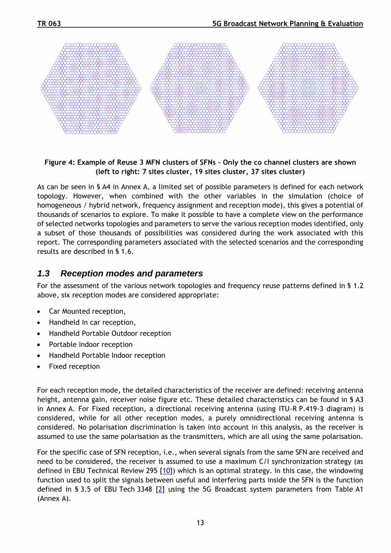
• In addition, for homogeneous cases, a mixed approach can be used for frequency assignment: the
mix is between MFN and SFN situations, i.e., MFN clusters of SFNs can be considered, the MFN
clusters adopting a frequency reuse 3 or 4, and all sites belonging to the cluster forming the same
SFN (with the same content transmitted in sync), as can be found in some operational broadcast
deployments. This approach provides a middle ground between a full SFN situation and a full MFN
situation for a given network topology. To preserve the regularity characteristics of the original
network topology, the clusters are formed from regular assemblies of sites: 7, 19, 37, …
Furthermore, to limit the extent of each cluster, the size of the clusters can be constrained
depending on the original network topology, e.g. only clusters of 7 sites for HPHT topology,
clusters of 7 or 19 sites for MPMT topology and clusters of 7, 19 or 37 sites for LPLT topology.
The figure below illustrates such clustering approaches in the case of frequency reuse 3 between the
clusters, showing only the clusters on the same frequency (clusters with red dots) as the central
cluster (cluster with green dots).
- Co-channel between two different regions (across regional borders inside a country or across national border between
two countries)
TR 063 5G Broadcast Network Planning & Evaluation
13
Figure 4: Example of Reuse 3 MFN clusters of SFNs – Only the co channel clusters are shown
(left to right: 7 sites cluster, 19 sites cluster, 37 sites cluster)
As can be seen in § A4 in Annex A, a limited set of possible parameters is defined for each network
topology. However, when combined with the other variables in the simulation (choice of
homogeneous / hybrid network, frequency assignment and reception mode), this gives a potential of
thousands of scenarios to explore. To make it possible to have a complete view on the performance
of selected networks topologies and parameters to serve the various reception modes identified, only
a subset of those thousands of possibilities was considered during the work associated with this
report. The corresponding parameters associated with the selected scenarios and the corresponding
results are described in § 1.6.
1.3 Reception modes and parameters
For the assessment of the various network topologies and frequency reuse patterns defined in § 1.2
above, six reception modes are considered appropriate:
• Car Mounted reception,
• Handheld In car reception,
• Handheld Portable Outdoor reception
• Portable Indoor reception
• Handheld Portable Indoor reception
• Fixed reception
For each reception mode, the detailed characteristics of the receiver are defined: receiving antenna
height, antenna gain, receiver noise figure etc. These detailed characteristics can be found in § A3
in Annex A. For Fixed reception, a directional receiving antenna (using ITU-R P.419-3 diagram) is
considered, while for all other reception modes, a purely omnidirectional receiving antenna is
considered. No polarisation discrimination is taken into account in this analysis, as the receiver is
assumed to use the same polarisation as the transmitters, which are all using the same polarisation.
For the specific case of SFN reception, i.e., when several signals from the same SFN are received and
need to be considered, the receiver is assumed to use a maximum C/I synchronization strategy (as
defined in EBU Technical Review 295 [10]) which is an optimal strategy. In this case, the windowing
function used to split the signals between useful and interfering parts inside the SFN is the function
defined in § 3.5 of EBU Tech 3348 [2] using the 5G Broadcast system parameters from Table A1
(Annex A).

5G Broadcast Network Planning & Evaluation TR 063
14
Regarding the propagation model, ITU R Recommendation P.1546 5 is used to predict wanted and
interfering field strengths from the various transmitters to the locations considered in the
simulations. As indicated in § A1 in Annex A, wanted signals are predicted for 50% of time, while
unwanted signals are predicted either using 1.75% of time (for location variation only simulations) or
any suitable percentage of time (for location and time variation simulations) as described in § 1.4.
1.4 Simulation methodology
The selection of parameters for a given network topology, the frequency reuse pattern (as described
in § 1.2) and the reception mode (as described in § 1.3) form a complete scenario to be considered
in a simulation run.
Whatever the simulation is, it is always based on the central “cell” of the network using a Monte
Carlo algorithm on a set of reception locations within this central cell:
• In the case of homogeneous networks with conventional reuse 1, 3 or 4, this cell is the central
cell of the network
• In the case of homogeneous networks with MFN clusters of SFNs, this cell corresponds to the set
of cells forming the central cluster
• In the case of hybrid networks, this cell corresponds to the central cell of the main layer
This set of reception locations is derived from the central cell using a regular grid. Whenever possible,
symmetry axes are used to reduce the number of such reception locations and speed up
computations.
Figure 5: Examples of central cell sampling – Reception locations indicated as ‘+’
Left: using symmetries (homogeneous networks with conventional reuse, hybrid networks)
Right: not using symmetries (homogeneous networks with MFN clusters of SFNs)
Each reception location is considered to form a small area of coverage of the network, the size of
which depends on the network topology5 as follows, due to computation time and memory constraints
limits linked to the inter site distance / central cell area:
• HPHT topology: small area of 500 m x 500 m (general case) or 1000 m x 1000 m (for MFN clusters
of SFNs)
5 In the case of hybrid networks, the topology to consider is the one of the main layer.
TR 063 5G Broadcast Network Planning & Evaluation
15
• MPMT topology: small area of 250 m x 250 m (general case) or 500 m x 500 m (for MFN clusters of
SFNs)
• LPLT topology for rural environments: small area of 150 m x 150 m or 250 m x 250 m (general
case) or 500 m x 500 m (for MFN clusters of SFNs)
• LPLT topology for urban/suburban environments: small area of 50 m x 50 m (general case) or
100 m x 100 m (for MFN clusters of SFNs).
At each reception location, a Monte Carlo algorithm is applied to derive SNR and SINR values for the
reception location and for a given percentage of locations (over the small area it represents) and
percentage of time (usually taken as 95% of locations / 99% of time respectively for broadcast
requirements). Two simulators were developed to achieve this computation:
• The first simulator does a unique Monte Carlo loop to derive statistics regarding location variation
only6 , introducing time variation aspects through the prediction model (wanted signals are
predicted for 50% of time, unwanted signals are predicted for 1.75% of time following the advice
by ITU-R Working Party 3K prescribed in the “Simple method” of ITU Document 6A/198 [11] that
individual interfering field strength computed using Recommendation ITU-R P.1546-5 at 1.75% of
time reflects the real correlation situation of interfering field strength and correspond to 1% of
time for the aggregated field strength.).
• The second simulator uses two nested Monte Carlo loops to derive statistics for location variation
and time variation of signals7. This produces a more consistent behaviour in predictions regarding
the wanted and unwanted parts of signal originating from a given source in SFNs, though at the
expense of a much-increased computation time due to the nested Monte Carlo loops. This
simulator has not been used for the derivation of the results shown in § 1.6 below due to the
excess runtime.
• The two simulators can examine both the data part (useful payload carried by the Physical
Multicast Channel – PMCH – of the 5G Broadcast system) and the signalling part (CAS – Cell
Acquisition Subframe), but the current simulations were only run on the data part, considering
that the signalling part is not a limiting factor in the effective reception of the signal8 .
The location variation only Monte Carlo algorithm is applied at each reception location as follows:
1. Compute the median wanted and unwanted signal levels from each site at the reception
location taking into account transmitter and receiver characteristics. Only signals
originating from sites on the same frequency as the central cell are taken account of in
this computation, since adjacent channel interference plays a secondary role.
2. For each location (Monte Carlo loop with N iterations, N taken as 10000 in the simulations).
a. Compute the shadowing factor (based on the applicable location standard deviation) for
each site.9
6 Simulator code available, on request for access, from https://git.ebu.io/smr-sdb/embms-simulations. 7 Simulator code available, on request for access, from https://git.ebu.io/smr-sdb/embms-simulations-time.
8 Despite its robustness, the CAS signal can only use the legacy LTE numerology (15 kHz with normal cyclic prefix, i.e.,
Tu = 66.67 µs, CP = 4.7 µs). This may have in impact on SFN reception, due to the very short CP duration, depending on the
behaviour of the receiver. 9 The shadowing factors are assumed to be uncorrelated between the sites. In some cellular network simulations, an
autocorrelation of the shadowing factors is indicated. This is not considered here.

5G Broadcast Network Planning & Evaluation TR 063
16
b. Correct the wanted / unwanted levels from each site with the corresponding shadowing
factor.
c. In case of SFN reception (reuse 1 or MFN clusters of SFN), apply the synchronisation
strategy10 to the signals originating from the sites in the SFN to derive wanted and
unwanted intra SFN signals.
d. Sum (using simple power sum) the wanted intra SFN signals and the unwanted (intra SFN
and out of SFN) signals separately to derive the SNR and SINR values for the current
location instance.
e. Accumulate each SNR and SINR location instance value in a table.
3. Once the Monte Carlo loop is over, derive a CDF of SNR and a CDF of SINR from the
accumulated values, and apply the location threshold (usually 95%) to derive the SNR and
SINR values reached for at least this percentage of locations, on the current reception
location.
Repeating the previous procedure over the whole set of reception locations allows a surface analysis
to be built, with charts showing coverage area versus specific available SNR and SINR values at the
wanted percentage of locations.
The following figures show an example of the application of such a procedure for a homogeneous
network simulation: Figure 6 shows the resulting computed SINR values for all reception locations
considered across a central cell, in the form of a heat map (reconstructed thanks to symmetries when
symmetries are used to derive the set of reception locations, using the original set of reception
locations otherwise); based on these values, and selecting relevant SINR values, one can also derive
a histogram representing the relative area covered for a given set of SINR values, as shown in Figure 7.
Figure 6: Computed SINR values for 95% of locations at reception locations across a central cell
Accumulating the resulting histogram of different scenarios (e.g., change in reuse factor, usage of
MFN clusters of SFNs, …) allows a performance comparison of the different scenarios to be made.
10 As theoretical networks are considered here, all transmitters in the SFN network are assumed to have an initial static
delay set to 0 µs.

TR 063 5G Broadcast Network Planning & Evaluation
17
Figure 7: Sample histogram resulting from the previous SINR computation,
for outstanding SINR values
The location and time variation Monte Carlo algorithm embeds the previous procedure in a time
instance loop and replaces the wanted / unwanted signal level generation by a generation for a given
time instance value.
The SNR and SINR values are accumulated along two dimensions and need two thresholding
procedures to derive the SNR and SINR values reached for the targeted time and location percentages
on each reception location (as already said, usually 99% of time / 95% of locations). The location and
time variation Monte Carlo algorithm is applied as follows at each reception location, since location
variation and time variation are independent random variables:
1. Generate M (number of Monte Carlo trials for the time variation; M was taken as 10000 in
the simulations) time instances for each transmitting site. The generation of those time
instances is based on the “General method” described in ITU Document 6A/198 [11], using
an extended version of Recommendation ITU-R P.1546-5 in the time domain, and α=1.
2. Generate N (number of Monte Carlo trials for the location variation; N was taken as 10000
in the simulations) shadowing components - i.e., location instances - for each transmitting
site (those trials are generated in the same way as for the location variation only
simulator).
3. For each time instance;
a. For each location instance;
i. Compute the received field strength from each transmitting site (only for the sites
on the same frequency as the central cell) at the current receiving location,
considering its time / location instances and the receiver characteristics.
ii. Derive the corresponding SINR (taking into account SFN self-interference when
needed and/or co channel interference when applicable) and store it in a matrix.
4. Using the SINR matrix;
a. Derive the CDF of SINR with respect to location, considering the target time percentage.
From this, derive the available SINR considering the target location percentage.

5G Broadcast Network Planning & Evaluation TR 063
18
b. Derive the CDF of SINR with respect to location, considering the target location
percentage. From this, derive the available SINR considering the target time
percentage.
The application of steps 4a and 4b should, in principle, return the same SINR value for the target
time and location percentages. However, due to the nesting of time and location loops in steps 1 to
3, reaching the same value is not guaranteed, considering the currently “reduced” number of trials
in both dimensions (nested Monte Carlo simulations usually require many loops in each dimension to
reach a stable result).
In practice, less than 0.5 dB difference was observed for the limited set of simulations that were
done using the location and time variation Monte Carlo algorithm. Decreasing this difference would
require significantly increasing the number of trials in both dimensions, putting an increased pressure
on runtime and memory usage (possibly even exhausting memory due to the necessary storage of the
time / location SINR matrix, unless specific measures are taken).
Using this algorithm provides a more optimistic result in terms of available SINR; for one given time
instance, the wanted and unwanted signals from one transmitting site are predicted using the exact
same percentage of time value using Recommendation ITU-R P.1546-5, hence producing a physically
consistent situation (rather than an artificial 50% of time for wanted signal and 1.75% of time for
unwanted signal from the same transmitting site).
The aggregation of the whole set of time instances generally results in a higher SINR on the considered
reception location. Of the limited set of simulations that was done, improvement in SINR at the worst
location was in the range of 1.5 – 3 dB for Fixed reception with reuse 1, depending on the topology,
and less than 0.2 dB for portable reception with reuse 1.
As this was done in the early stages of the work, further assessment would be necessary to fully
qualify the difference resulting from using the location and time variation Monte Carlo algorithm
compared with the location only Monte Carlo algorithm, in particular over the whole coverage area
and not only at the worst location. For the time being, and as previously explained, the results
presented in the following sections are based on the location variation only Monte Carlo algorithm.
1.5 Coverage of national or regional border areas
1.5.1 Background
This section shows the impact of single frequency operation across regional or national boundaries
with different content in each region.
This topic was studied as part of work associated with CEPT TG6, in around 2013, which explored the
impact of single frequency use across regional boundaries primarily for Fixed reception [12]. At that
time, it was shown that it was not possible to operate reuse 1 networks in border areas and provide
complete coverage for Fixed reception.
As the TG6 work only considered Fixed reception, similar work has been done in this section to cover
some of the scenarios being considered as part of the 5G Broadcast studies; namely,
• HPHT, MPMT and LPLT network structures
• Mobile (Car Mounted) reception

TR 063 5G Broadcast Network Planning & Evaluation
19
For the above scenarios, the reduction in availability (coverage) in cells adjacent or close to the
border was investigated for single frequency operation across a regional or national boundary with
different content in each region. In line with the approach taken in the TG6 work, the impact on
cells/sectors, adjacent or near to a border has been assessed.
The case where an area is partly enveloped by a different region has been modelled. This has been
represented by dividing the modelled area into 4 quadrants. Of these quadrants, 3 represent
interfering regions and the fourth (lower left) is the wanted region. (see Figure 9a below and §§ C1.1,
C2.1 and C3.1 in Annex C). In this situation, a wanted cell has interfering cells adjacent on 4 faces.
The impact has been reported as a CDF of the SINR available across the area and a heat map of
available SINR.
In addition, the case where a regional boundary is straight has been modelled with two sub cases:
Vertical North South boundary (see §§ C1.3, C2.3 and C3.3 of Annex C) and Horizontal East West
boundary (see §§ C1.2, C2.2 and C3.2 of Annex C). As we are working with networks based on
hexagonal cells there is a slight difference in interference between the two cases - one has an
interfering cell adjacent on 3 faces of the hexagon, the other an interfering cell on two faces.
1.5.2 Results
Example results are provided in Figures 8 & 9. The full set of results for the three different network
topologies, Car Mounted (i.e. mobile) reception and a 5 MHz bandwidth are provided in Annex C.

5G Broadcast Network Planning & Evaluation TR 063
20
Figure 8: CDF for LPLT - corner regional boundary
Figure 9a: Network Geometry corner (the green cells are the wanted region,
red cells are the interfering region. The assessed cell is the central cell)
Figure 9b: Resulting SINR heat map for HPHT case
1.5.3 Discussion
The results (Annex C) show that for all network topologies, HPHT, MPMT & LPLT, coverage in border
areas is reduced when compared with coverage away from the border. Coverage is compromised in
a band running along the border.
• For HPHT networks, the first and second cells from the border are mainly impacted, while the
third cell suffers almost no impact on its coverage as part of a reuse 1 national network. In terms

TR 063 5G Broadcast Network Planning & Evaluation
21
of distance from the border, this represents roughly 2x ISD (Inter-site Distance of the HPHT
network). For an ISD of 80 km, most considered in the current simulations, this represents 160 km.
This order of distance would still allow a reuse 1 inside, but not across the whole territory of, a
large country (France, Germany, Spain, Poland, etc.) but not in small countries (Luxembourg,
Belgium, Croatia, etc.)
• For MPMT and LPLT networks, the first, second and third cells from the border are impacted. The
impact is expected to be minimal on the fourth cell. In terms of distance from the border, this
represents 3x ISD. For an MPMT ISD of 20 km, this represents 60 km from the border. For an LPLT
ISD of 12 km, this represents 36 km. These distances are sufficiently low for medium size
countries to allow some reuse 1 inside their territories.
A straightforward solution in such border areas is to use different frequencies for SFNs that transmit
different content (across national or regional borders). For LPLT and MPMT this probably means a
frequency reuse of 3 is required. Figure 10 shows an illustration of using MFN with reuse 3 on both
sides of a border while still using SFN inside each area at a distance from the border. For HPHT, given
the ISD, a frequency reuse of 4 would be required when regions or countries are comparable in size
to the coverage area of a station.
It may be possible to reduce the size of the impacted area by implementing closed SFNs11. This has
not been investigated but it is believed that while it would reduce the size of the impacted area, it
would not entirely eliminate the problem.
11 A Closed SFN uses directional antenna patterns at transmitters located at its edge, oriented towards the centre of the
SFN, to reduce the outgoing interference to neighbouring co-channel networks.

5G Broadcast Network Planning & Evaluation TR 063
22
Figure 10: Illustration of an MFN at the border area with reuse 3 while SFN
is used inside each country at a distance from the border
1.5.4 Conclusion
Regardless of the network configuration it is not possible to operate reuse 1 networks in border areas
and provide contiguous coverage. In border areas, full coverage requires either a higher frequency
reuse, i.e., to use Multiple Frequency Networks (MFN) in the concerned border areas, or a solution
to reduce the size of co channel interference by implementing closed SFNs.
1.6 Results
The full set of detailed results can be requested from the EBU (5G planning simulation results). The
following provides analysis for each use case (Car Mounted, Handheld Portable outdoor, Handheld
In-Car and Fixed reception).
1.6.1 Networks assessment for Car-Mounted reception
Effect of the Cyclic Prefix and the frequency reuse on the coverage
Figures 11 & 12 show the percentage of surface covered for different target SINR values for Car
Mounted reception using HPHT with 300 µs cyclic prefix (CP) and 200 µs CP respectively (see Table A1
for the different possibilities offered by 5G Broadcast).
Figures 13 & 14 show the same type of results but using MPMT. The main characteristics of these
homogeneous networks are shown in Table 2.
Figure 11 Figure 12

TR 063 5G Broadcast Network Planning & Evaluation
23
Figure 13 Figure 14
Table 2: The main parameters of the homogeneous HPHT and MPMT networks
Layer ISD (km) Antenna height
a.g.l. (m)
EIRP
(in a 5 MHz channel)
Site density
(per 10000 km2 - see note)
HPHT 80 300 79.9 dBm/98 kW 1.8
MPMT 20 80 59.6 dBm/912 W 28.9
Note: Based on the ISD figures in Tables1 & 2.
Observations:
1. The coverage of HPHT and MPMT networks for Car Mounted reception is mainly
noise-limited due to low signal levels, this is evident from the low SNR figures obtained in
the simulations. However, the coverage of reuse 1 (Single Frequency) Network is
significantly better than reuse 3 and 4 (MFNs), due to the constructive contribution of
signals inside the CP. The coverage of reuse 3 and 4 networks can be improved with the
use of reuse 3 and 4 MFN clusters of SFNs (7 cells in HPHT, 19 cells in MPMT) compared to
reuse 3 and 4 “pure” MFNs, due to both the constructive contribution of signals inside the
CP and the reduction in co channel interference with the increased co channel separation
distance.
2. Compared to a CP of 200 µs, increasing the CP to 300 µs improves, to some extent, the
Car Mounted coverage of HPHT and of MPMT reuse 1 as it allows more signals to be
constructive and fewer signals to be interfering; but the main limitation for the coverage
remains the lack of signal level. Similarly, there is a small improvement in the coverage
of reuse 3 and 4 MFN clusters of SFNs. As expected, increasing the CP does not have an
impact on reuse 3 and 4 coverages, which correspond to “pure” MFNs.
The coverage improvement with a CP of 300 µs should be considered mindful of the
limitation that it would impose on the speed of movement of the receivers (see § 1.7.2 on
Doppler performance). The use of 200 µs for the CP, on the other hand, allows for
reception at normal vehicle speeds.
3. An HPHT network alone would offer 10 dB SINR (in 5 MHz) for Car Mounted reception in
87.1% to 96.1% of the target coverage area with 200 µs CP, and slightly more (90.6% to
100%) with 300 µs CP. For 15 dB SINR and higher, the improvement in coverage with 300 µs
CP is more significant.
4. An MPMT network alone would offer 15 dB SINR (in 5 MHz) in 86.6% to 98.1% of the target
coverage area with 200 µs CP, and slightly more (86.8% to 100%) with 300 µs CP. For 20 dB
SINR and higher, the improvement in coverage with 300 µs CP is more significant.
In summary, used individually, homogeneous HPHT and MPMT network types have limitations in terms
of coverage and available SINR for Car Mounted reception.
The use of hybrid HPHT+MPMT networks is therefore now evaluated.
Use of Hybrid network (HPHT+MPMT) to further improve the coverage and effect of increasing
the EIRP

5G Broadcast Network Planning & Evaluation TR 063
24
Figures 15 & 16 show the percentage of surface covered for different target SINR values for Car
Mounted reception using a hybrid HPHT+MPMT network having the main characteristics shown in
Table 3 (see illustration of Hybrid networks in § 1.2).
A CP of 200 µs was adopted for these hybrid networks, to favour high speed mobile reception. In
addition, the effect of increased EIRP was tested by increasing the MPMT EIRP by 7 dB (indicated with
“Revised Situation” in Figure 16 compared to the “Base Situation” of Figure 15 where no increase of
the MPMT EIRP is considered). This EIRP adjustment would be needed to overcome the
self-interference effect in the case the Hybrid network in SFN mode.
To better visualise the improvement achieved from the use of a Hybrid Network, Figures 17 & 18
show a comparison of HPHT layer alone, MPMT layer without the HPHT, MPMT alone (full) and Hybrid
HPHT+MPMT. Both Figures 17 & 18 consider a 7 dB increase in EIRP for the full MPMT Network and for
the MPMT component of the Hybrid Network.
Figure 15 Figure 16
Figure 17 Figure 18
Table 3: The main parameters of the Hybrid Network
Layer ISD (km) Antenna height
a.g.l. (m)
EIRP
(in a 5 MHz channel)
Site density
(per 10000 km2 - see note)
HPHT 80 300 79.9 dBm/98 kW 1.8
MPMT Base
situation 23.1 80 59.6 dBm/912 W 21.6

TR 063 5G Broadcast Network Planning & Evaluation
25
MPMT Revised
situation 23.1 80 66.6 dBm/4.6 kW 21.6
Note: Based on the ISD figures in Tables 1 & 3.
Observations:
1. Compared to homogeneous networks in Figures 12 & 14 (reuse 1 pure SFN or reuse 3 or 4
pure MFNs), the hybrid HPHT+MPMT networks in Figure 15 offer a significant increase in
coverage for the higher SINR figures (15 dB and above). The improvement shown in
Figure 16 is even more significant with the 7 dB increase of EIRP of the MPMT layer
transmitters.
2. The increase of the EIRP of the MPMT layer offers a large improvement in the coverage,
even with the MPMT layer alone. Figures 17 & 18 indicate that a full MPMT layer (using
revised characteristics from Table 3) matches the overall coverage of the Hybrid network
for a SINR up to 15 dB. However, for a SINR above 15 dB, the hybrid network exceeds the
coverage of any individual homogeneous layer. In particular, a hybrid network with reuse 4
could achieve 20 dB SINR in 90% of the target area.
In summary, a hybrid HPHT+MPMT or a full MPMT 5G Broadcast network with the characteristics
shown in Table 3 (MPMT Revised situation) can offer a SINR of 15 dB (in 5 MHz) to Car Mounted
receivers in 100% of the target coverage area. This network can be operated either as a general basis
or as a solution with reuse 3 or 4 close to the national or regional border areas. The density of sites
in such a network is around 21.6 sites per 10000 km² (1.8 HPHT + 19.8 MPMT sites per 10000 km2).
Use of LPLT homogeneous network for Car Mounted reception
Figures 19 & 20 show the percentage of surface covered for different target SINR values for Car
Mounted reception using LPLT in Suburban and Urban areas, respectively. The main characteristics
of these homogeneous networks are shown in Table 4.
Figure 19 Figure 20
Table 4: The main parameters for the homogeneous LPLT networks
Layer ISD (km) Antenna height
a.g.l. (m)
EIRP
(in a 5 MHz channel)
Site density
(per 10000 km2 - see note)
LPLT 3 30 57 dBm/500 W 1283
Note: Based on the ISD figures in Tables 1 & 4.
Observations:
5G Broadcast Network Planning & Evaluation TR 063
26
A CP of 100 µs is suitable for LPLT. Reuse 1 offers the best coverage, ensuring 25 dB SINR in 100% of
the target coverage area for Car Mounted reception for both urban and suburban environments.
For the coverage close to national or regional borders, reuse 3 and 4 with MFN clusters of SFNs (19 or
37 cells) can also offer quite high coverage figures: with reuse 4 MFN clusters of SFNs in urban areas,
an area coverage of 92% can be achieved for a 20 dB target SINR.
In summary, an LPLT 5G Broadcast network with the main characteristics shown in Table 4 can offer
an SINR of 15 dB (in 5 MHz) to Car Mounted receivers in 100% of the target coverage area or 20 dB in
92% of the area for both suburban and urban environments. This network can be operated with
reuse 1 inside the national territory, if possible, and with reuse 3 or 4 close to the national or regional
border areas, using MFN clusters of SFNs with 37 cells or more.

TR 063 5G Broadcast Network Planning & Evaluation
27
1.6.2 Networks assessment for Handheld Portable Outdoor reception
Effect of the Cyclic Prefix and the frequency reuse on the coverage
Figures 21 & 22 show the percentage of surface covered for different target SINR values for Handheld
Portable Outdoor reception using HPHT with 300 µs CP and 200 µs CP respectively. Figures 23 & 24
show the same type of results but using MPMT. The main characteristics of these homogeneous
networks are shown in Table 2, above.
Figure 21 Figure 22
Figure 23 Figure 24
Observations:
1. Figures 21 & 22 show that the coverage of HPHT networks for portable outdoor reception are
severely limited by noise due to low signal levels, this is evident from the low SNR figures
obtained in the simulations and is due to the high signal margins required for portable
reception with handheld receivers. This explains the absence of effect of increasing the CP
from 200 µs (Figure 22) to 300 µs (Figure 21).
2. Figures 23 & 24 show that, for reuse 1, the coverage of MPMT networks is better than that of
HPHT but is still quite limited in terms of achievable SINR figures. As in the case of
Car-Mounted reception (Figures 13 & 14, above), the coverage can be significantly improved
with the use of reuse 3 and MFN clusters of SFNs (7 cells in HPHT, 19 cells in MPMT), compared
to reuse 3 and 4 “pure” MFNs, due to the constructive contribution of signals inside the Cyclic
Prefix and the reduction in co-channel interference with the increased co-channel distance.

5G Broadcast Network Planning & Evaluation TR 063
28
In summary, used individually, HPHT and MPMT network types have limitations in terms of coverage
and available SINR for Handheld Portable Outdoor reception.
The use of hybrid HPHT+MPMT networks is therefore now evaluated.
Use of Hybrid network (HPHT+MPMT) to further improve the coverage and effect of increasing
the EIRP
Figures 25 & 26 show the percentage of surface covered for different target SINR values for Handheld
Portable Outdoor reception using a hybrid HPHT+MPMT network having the main characteristics
shown in Table 3, above (see illustration of Hybrid networks in § 1.2). A CP of 200 µs was adopted for
these hybrid networks for consistency with the simulations for Car-Mounted reception. In addition,
the effect of increased EIRP was tested by increasing the MPMT EIRP by 7 dB (indicated “Revised
Situation” in Figure 25, compared to the “Base Situation” of Figure 26, where no increase of the
MPMT EIRP is considered).
As above, to better visualise the improvement achieved from the use of a Hybrid Network,
Figures 27 & 28 show a comparison of HPHT layer alone, MPMT layer without the HPHT, MPMT alone
(full) and Hybrid HPHT+MPMT. Both Figures 27 & 28 consider a 7 dB increase in EIRP for the full MPMT
Network and for the MPMT component of the Hybrid Network.
Figure 25 Figure 26
Figure 27 Figure 28
Observations:

TR 063 5G Broadcast Network Planning & Evaluation
29
The Hybrid networks offer significantly improved coverage for Handheld Portable Outdoor reception
compared to the homogeneous networks. In addition, increasing the EIRP of the MPMT layer by 7 dB
(from 59.6 to 66.6 dBm) allows for a full area coverage with 10 dB SINR or around 50% coverage with
15 dB SINR.
In summary, a hybrid HPHT+MPMT 5G Broadcast network with the characteristics shown in Table 3
(MPMT Revised situation) can offer a SINR of 10 dB (in 5 MHz) to Handheld Portable Outdoor receivers
in 100% of the target coverage area or 15 dB (in 5 MHz) in around 50% of the target coverage area.
This network can be operated either as a general basis or as a solution with reuse 4 close to the
national or regional border areas. The density of sites in such a network is around 21.6 sites per
10000 km² (1.8 HPHT + 19.8 MPMT sites per 10000 km2).
Use of LPLT homogeneous network for Handheld Portable Outdoor reception
Figures 29 & 30 show the percentage of surface covered for different target SINR values for Handheld
Portable Outdoor reception using LPLT in Suburban and Urban areas, respectively. The main
characteristics of these homogeneous networks are shown in Table 4. The detailed results are shown
in Annex C.
Figure 29 Figure 30
Observations:
A CP of 100 µs is suitable for LPLT. Reuse 1 offers the best coverage, ensuring 20 dB in 100% of the
target coverage area in suburban or 15 dB in urban area for Handheld Portable Outdoor reception.
For the coverage close to national or regional borders, reuse 3 and 4 MFN clusters of SFNs (19 or 37
cells) can also offer quite high coverage figures: with reuse 4 MFN clusters of SFNs in urban areas,
area coverage of 92% can be achieved for a 15 dB target SINR.
In summary, an LPLT 5G Broadcast network with the main characteristics shown in Table 4 can offer
a SINR of 15 dB (in 5 MHz) to Handheld Portable Outdoor receivers in 100% of the target coverage
area in suburban environment and 92% to 100% in urban environment. This network can be operated
with reuse 1 inside the national territory, if appropriate, and with reuse 4 close to the national or
regional border areas, using MFN clusters of SFNs with 37 cells.
1.6.3 Networks assessment for Handheld In Car reception
Use of LPLT homogeneous network for Handheld In Car reception
Figures 31 & 32 show the percentage of surface covered for different target SINR values for Handheld
In Car reception using LPLT in Suburban and Urban areas, respectively. The main characteristics of
these homogeneous networks are shown in Table 4.

5G Broadcast Network Planning & Evaluation TR 063
30
Figure 31 Figure 32
Observations:
The additional margin required for Handheld In Car reception compared with Car Mounted reception
imposes further difficulties to insure a sufficient area coverage. For this reason, only the LPLT
network type has been evaluated.
Similar to the use of LPLT network for Car Mounted reception, a CP of 100 µs is suitable. Reuse 1
offers the best coverage, ensuring 15 dB in 100% of the target coverage area for Handheld In Car
reception for suburban environment and 10 dB in 100% of the target coverage area for urban
environment. Reuse 4 with MFN clusters of SFNs (37 cells) can offer quite high coverage figures,
reaching 98.5% area coverage for SINR of 10 dB in suburban areas. This coverage is however limited
to 77.8% for SINR of 10 dB in urban areas.
In summary, an LPLT 5G Broadcast network with the main characteristics shown in Table 4 can offer
a SINR of 10 dB (in 5 MHz) to Handheld In Car receivers in 98.5% to 100% of the target coverage area
in a suburban environment and 77.8% to 100% in an urban environment. This network can be operated
with reuse 1 inside the national territory, if appropriate, and with reuse 4 close to the national or
regional border areas, using MFN clusters of SFNs with 37 cells.
1.6.4 Networks assessment for Fixed Rooftop reception
Effect of the frequency reuse on the coverage
Figures 33 & 34 show the percentage of surface covered for different target SINR values for Fixed
Rooftop reception using HPHT and MPMT network, respectively. Only a CP of 300 µs was used in this
assessment. The main characteristics of these homogeneous networks are shown in Table 2.
Figure 33 Figure 34
Observations:

TR 063 5G Broadcast Network Planning & Evaluation
31
Figures 33 & 34 show that HPHT and MPMT networks can offer up to 25 dB SINR with a near full area
coverage for Fixed Rooftop reception either with reuse 1 or with reuse 4 MFN clusters of SFNs (7 cells
in HPHT, 19 cells in MPMT). The area coverage rate exceeds 99.5% with HPHT and 97.8% with MPMT.
In summary, an HPHT or an MPMT 5G Broadcast network with the main characteristics shown in
Table 2 can offer an SINR of 25 dB (in 5 MHz) to Fixed Roof Top receivers in 99.5% and 97.8% of the
target coverage area, respectively. This network can be operated with reuse 1 inside the national
territory, if appropriate, and with reuse 3 for HPHT or 4 for MPMT close to the national or regional
border areas, using MFN clusters of SFNs with 7 cells for HPHT and 19 cells for MPMT. Reuse 4 MFN
clusters of SFNs offers an equivalent area coverage to reuse 1 full SFN.
1.7 Specific analysis
1.7.1 Impact of practical antenna pattern
The generic studies to assess 5G Broadcast coverage are based on idealised, omnidirectional antenna
patterns, where networks use HPHT and MPMT infrastructure and an optimized tri-sector pattern for
LPLT sites. However, the real-world implementation of 5G Broadcast could be based both on existing
antennas and on new antennas, where it is possible and cost-effective to install such new antennas.
For the range of site topologies considered in this report (LPLT, MPMT and HPHT) the currently
implemented antennas have been designed to meet existing network requirements and direct use by
5G Broadcast may lead to sub-optimum performance.
For sites that are currently in use for conventional Broadcasting, a single antenna array comprising
several individual radiating elements provides uniform azimuthal coverage over the required arc;
often a full 360 degrees. In reality, and due to constraints in practical antenna design, a ripple of up
to 4 dB is the best that can generally be achieved, and the existing broadcast sites may be considered
to be optimised for conventional broadcasting and also for 5G Broadcast.
For sites that are currently used by the Mobile Network, the situation is rather different. Generally,
the antennas are constructed from arrays of elements providing 120 degree ‘sector’ azimuthal
coverage. Where coverage is required over a full 360 degrees, three such antennas are mounted at
120-degree intervals around the structure. Where specific geographical areas are targeted, sector
antennas may be oriented accordingly. The existing unicast mobile network can select and energise
these sector antennas independently and so any interaction between adjacent sectors is not
important – the base station scheduler may ensure that adjacent antennas are not used on the same
resource block at the same time. However, if this arrangement of sector antennas is simultaneously
powered from a single transmitter, as may be the case for 5G Broadcast applications, the interaction
between adjacent antennas should be considered as this may lead to a compromise in the overall
performance [13].
The sector antennas typically used by mobile systems are not designed to operate as arrays. If so
used for 5G Broadcast, such arrays would have deep nulls in the radiated pattern, which may
compromise coverage. Measures to mitigate this loss in coverage may be required. Existing broadcast
antenna systems have already been optimised for coverage. See Annex E for more information.
The impact on coverage could be reduced by increasing the EIRP, adopting an increased phase delay
between sector antennas (cyclic delay diversity), a combination of the two or building a new antenna
with a better pattern. Each has a cost implication that needs to be weighed against the potential
loss in coverage. Again, see Annex E for more information.
5G Broadcast Network Planning & Evaluation TR 063
32
1.7.2 Estimate of Doppler performance
For a 5G Broadcast system targeting mobile reception, system Doppler performance is important as,
via the carrier spacing and hence the choice of Cyclic Prefix (CP), it can drive the network design.
Doppler is an issue for broadcast systems. DAB systems largely avoid the problem because of the low
frequency employed, around 200 MHz. DTT systems are typically designed for Fixed reception where
Doppler is generally not a problem. DTT systems designed for portable/mobile reception (as, for
example, in Germany) employ increased carrier spacing (fewer carriers i.e., larger frequency spacing
between carriers) and hence smaller SFN size along with more dense networks (reduced spacing
between transmitters).
The ISD in an SFN is dependent on the length of the CP. The larger the ISD, the longer the CP needs
to be, and correspondingly a longer symbol time is needed. However, longer symbol time, which is a
function of the inverse of the carrier spacing, will result in degraded Doppler performance and lower
speed limits for mobile reception.
Without doing detailed and complicated link-level simulations, the calculation of Doppler
performance for OFDM-based broadcast systems can be estimated from methods described in [16],
which investigate the Inter Carrier Interference (ICI, or FFT leakage) as a function of Doppler. This
work focused on DVB-T/T2 but the methodology is applicable to any OFDM system, including 5G
Broadcast.
The report of this work contains an extensive mathematical analysis but ends up with a “simple”
formula for an OFDM system with 1 kHz carrier spacing:
𝐶 𝐼⁄ = 58.6 − 20 𝑙𝑜𝑔10 (𝑓𝑑) dB
Where: fd is the Doppler frequency in a Rayleigh fading channel in Hertz.
For example, 100 Hz Doppler results in a "C/I" = 58.6 - 40 = 18.6 dB. If the required C/N of the system
is known, it is easy to calculate the C/N degradation. Usually, a 3 dB increase of required C/N is used
when presenting the Doppler frequency limits and corresponding speed limits. The maximum
theoretical Doppler may also be calculated.
Modifications:
• Changing the FFT (symbol time) will change the constant 58.6 in the equation. For example,
500 Hz carrier spacing (16k FFT) will reduce the value by 6 dB, and for 250 Hz carrier spacing (32k
FFT) by 12 dB, resulting in constant values of 52.6 dB and 46.6 dB, respectively.
• Other symbol times may be scaled correspondingly; for example, a factor 2 corresponds to 6 dB,
means that, for example, a factor of 1.8 should be 4 (6 dB in linear scale) x 1.8/2.0. Converted
back to dB scale the correction to 58.6 would be 5.6 dB.
ICI is, however, not the only limitation. Additionally, the limitations created by the channel
estimation, CE, (determined by the Pilot Patterns) need to be determined. These Scattered Pilot
Patterns are used for channel estimation in the receiver, in frequency and in time12. But in the case
of 5G Broadcast the FFT leakage (ICI) seems to be the main limitation, at least for the OFDM variants
of interest in SFNs.
In the tables below the maximum Doppler and speed limitation for 5G Broadcast are derived for three
proposed 5G Broadcast modes operating at 600 MHz.
12 The repetition pattern in frequency is denoted Dx or Df, while the repetition pattern in time is denoted Dt or Dy
TR 063 5G Broadcast Network Planning & Evaluation
33
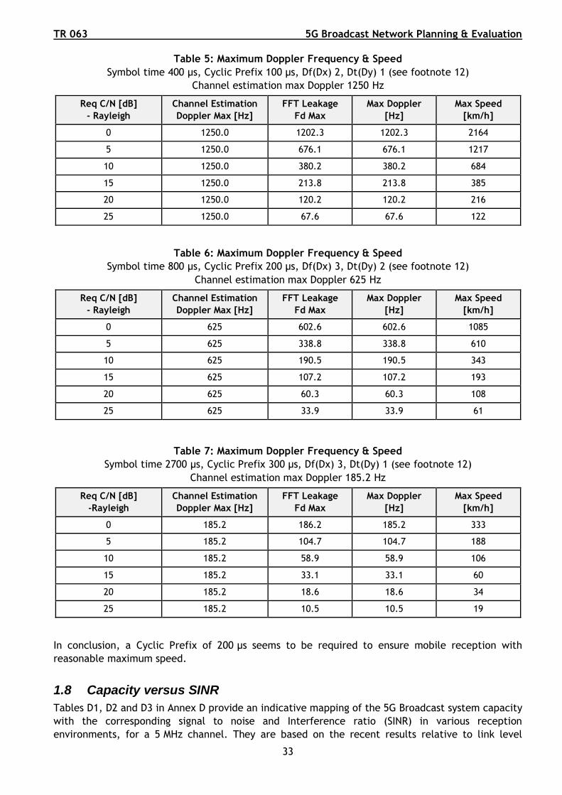
Table 5: Maximum Doppler Frequency & Speed
Symbol time 400 µs, Cyclic Prefix 100 µs, Df(Dx) 2, Dt(Dy) 1 (see footnote 12)
Channel estimation max Doppler 1250 Hz
Req C/N [dB]
- Rayleigh
Channel Estimation
Doppler Max [Hz]
FFT Leakage
Fd Max
Max Doppler
[Hz]
Max Speed
[km/h]
0 1250.0 1202.3 1202.3 2164
5 1250.0 676.1 676.1 1217
10 1250.0 380.2 380.2 684
15 1250.0 213.8 213.8 385
20 1250.0 120.2 120.2 216
25 1250.0 67.6 67.6 122
Table 6: Maximum Doppler Frequency & Speed
Symbol time 800 µs, Cyclic Prefix 200 µs, Df(Dx) 3, Dt(Dy) 2 (see footnote 12)
Channel estimation max Doppler 625 Hz
Req C/N [dB]
- Rayleigh
Channel Estimation
Doppler Max [Hz]
FFT Leakage
Fd Max
Max Doppler
[Hz]
Max Speed
[km/h]
0 625 602.6 602.6 1085
5 625 338.8 338.8 610
10 625 190.5 190.5 343
15 625 107.2 107.2 193
20 625 60.3 60.3 108
25 625 33.9 33.9 61
Table 7: Maximum Doppler Frequency & Speed
Symbol time 2700 µs, Cyclic Prefix 300 µs, Df(Dx) 3, Dt(Dy) 1 (see footnote 12)
Channel estimation max Doppler 185.2 Hz
Req C/N [dB]
-Rayleigh
Channel Estimation
Doppler Max [Hz]
FFT Leakage
Fd Max
Max Doppler
[Hz]
Max Speed
[km/h]
0 185.2 186.2 185.2 333
5 185.2 104.7 104.7 188
10 185.2 58.9 58.9 106
15 185.2 33.1 33.1 60
20 185.2 18.6 18.6 34
25 185.2 10.5 10.5 19
In conclusion, a Cyclic Prefix of 200 µs seems to be required to ensure mobile reception with
reasonable maximum speed.
1.8 Capacity versus SINR
Tables D1, D2 and D3 in Annex D provide an indicative mapping of the 5G Broadcast system capacity
with the corresponding signal to noise and Interference ratio (SINR) in various reception
environments, for a 5 MHz channel. They are based on the recent results relative to link level

5G Broadcast Network Planning & Evaluation TR 063
34
simulations of different 5G Broadcast configurations presented in [14] for various SINR values. The
link level simulations presented in [14] do not cover all configuration cases and all reception modes.
Moreover, for Fixed reception, they correspond to the use of one antenna, while for portable / mobile
reception two antennas are assumed, leading to diversity gain in the receivers. As such they provide
an upper bound on the capacity associated with a given SINR value.
Based on the information of Annex D, Tables 8 to 10 give an indicative mapping of the key SINR values
reflected in § 1.6 with the corresponding capacity (upper bound) for the different CP values and
target reception modes.
Table 8: Upper bound on capacity for 100 µs CP and key SINR values
SINR (dB)
Car Mounted
Handheld In car
Capacity (Mbit/s)
in a 5 MHz channel
Handheld Portable Outdoor
Portable Indoor
Handheld Portable Indoor
Capacity (Mbit/s)
in a 5 MHz channel
Fixed Rooftop
Capacity (Mbit/s)
in a 5 MHz channel
0 - - N/A
5 2.161 2.161 N/A
10 4.282 4.844 N/A
15 7.543 7.792 N/A
20 10.413 11.162 N/A
25 12.262 13.198 N/A
Table 9: Upper bound on capacity for 200 µs CP and key SINR values
SINR (dB)
Car Mounted
Handheld In car
Capacity (Mbit/s)
Handheld Portable Outdoor
Portable Indoor
Handheld Portable Indoor
Capacity (Mbit/s)
Fixed Rooftop
Capacity (Mbit/s)
0 - - -
5 2.161 2.535 2.535
10 4.282 4.844 4.844
15 7.043 7.792 7.792
20 8.915 11.162 11.162
25 (> 9.664) (>12.262) (>12.262)

TR 063 5G Broadcast Network Planning & Evaluation
35
Table 10: Upper bound on capacity for 300 µs CP and key SINR values
SINR (dB)
Car Mounted
Handheld In car
Capacity (Mbit/s)
Handheld Portable Outdoor
Portable Indoor
Handheld Portable Indoor
Capacity (Mbit/s)
Fixed Rooftop
Capacity (Mbit/s)
0 - - -
5 - 3.097 3.097
10 - 6.201 6.201
15 - 10.304 10.304
20 - 15.239 13.770
25 - (>15.239) (>15.239)
1.9 Conclusions from simulation results on theoretical Networks
It should be possible to ensure 15 dB SINR in 5 MHz for 5G Broadcast Car Mounted receivers with full
rural area coverage using a Hybrid HPHT+MPMT network with HPHT EIRP similar to current typical
DTT HPHT networks and with MPMT EIRP slightly higher than current typical DTT MPMT networks.
Reuse 1 should be used where possible and reuse 3 or 4 MFN clusters of SFNs should be used where
reuse 1 cannot be implemented, typically at regional and national borders. A CP of 200 µs is
recommended to allow reception at normal vehicle speeds. In these conditions, in a 5 MHz channel,
a capacity up to 7.043 Mbit/s could be achieved (1.4 b/s/Hz).
A full LPLT network could provide 15 dB SINR in 5 MHz for 5G Broadcast Car Mounted receivers with
full urban and suburban area coverage. Considering the large site density for this type of network
(1283 sites per 10000 km2), its use may be limited to the coverage of urban and suburban areas with
reuse 1, with rural areas being more efficiently covered by Hybrid HPHT+MPMT networks as described
above, with a site density around 21.6 sites per 10000 km2. The same capacity as above, i.e., up to
7.043 Mbit/s, could be achieved.
5G Broadcast Handheld In Car reception with 15 dB SINR is not achievable across a full area for any
of the analysed network types. The coverage for this type of reception would be limited to best
effort.
The same Hybrid HPHT+MPMT described above would also ensure 15 dB SINR in 5 MHz for Handheld
Portable Outdoor reception in 50% of rural areas. It should be noted that the coverage in terms of
population in rural areas could be higher than the area coverage if the choice of the sites is made
adequately.
A complementary reuse 1 LPLT network, as described above, is necessary in suburban and urban
areas to ensure 15 dB SINR for Handheld Portable Outdoor in these areas. In these conditions and
using the same MCS as for Car Mounted, a capacity up to 7.043 Mbit/s could be achieved. Otherwise,
if a dedicated network for Handheld Portable Outdoor reception is selected, a capacity up to
7.792 Mbit/s could be achieved.
Fixed Rooftop reception of 5G Broadcast with 15 dB SINR in 5 MHz should be possible from the
networks described above, at least with the same coverage areas as for Car Mounted and Handheld
Portable receptions. However, if rooftop reception is primarily targeted, HPHT or MPMT networks
currently used for DTT could ensure 25 dB in 5 MHz for 5G Broadcast Fixed Rooftop reception with
near full area coverage.

5G Broadcast Network Planning & Evaluation TR 063
36
Near full population coverage would also be expected with these networks. Reuse 1 could be used
when possible and reuse 3 or 4 MFN clusters of SFNs could be used when reuse 1 cannot be
implemented, especially at regional and national borders. A 300 µs CP may be required, which is not
suitable for mobile reception. In these conditions, a dedicated network would be needed for this
reception mode.
The available information on link level simulations does not allow assessment of what capacity could
be achieved. It is only possible to say that this capacity will exceed 15.239 Mbit/s in 5 MHz.
2. Real Networks
One of the key drivers for broadcasters’ and broadcast network providers’ interest in adopting 5G
Broadcast is making their content available to handheld devices such as mobile phones and tablets.
A critical question is whether the existing broadcast infrastructure used for DAB or DTT, possibly
complemented with cellular type networks, can be used to provide such handheld services using 5G
Broadcast. Therefore, simulations have been carried out based on existing real network sites to see
if this could be an option and under what conditions this would be feasible.
Two implementations of 5G Broadcast networks based on existing broadcast infrastructure have been
modelled. The first network, in Italy, is based upon one developed for the former DVB-H
implementation on the existing DVB-T channel 38 national SFN, augmented by mobile operator sites.
The second network is based on the national DAB network deployed in Denmark.
2.1 Italy
The coverage of a 5G Broadcast network based on the existing DVB-T channel 38 SFN network13
augmented by additional mobile network operator sites has been assessed.
2.1.1 5G Broadcast sites
This network, consisting of 821 sites of a BNO (Broadcasting Network Operator), is a real existing
national network designed for Fixed reception that provides useful roof top coverage to more than
94% of the population. It consists of a mixture of HPHT, MPMT and LPLT.
To extend coverage for handheld/mobile use, the network was augmented by two sets of existing
Mobile Network Operator (MNO) sites. The first set (1037) of MNO sites is a large part of those that
were used in one of the two former DVB-H networks in Italy. A second set of (1253) MNO sites is
considered to complete the coverage, see Table 11.
Table 11: Sites considered for the 5G Broadcast Network in Italy
Sites North South
Italy (reg. 1-10) (reg. 11-20)
BNO 458 363 821
MNO part #1 581 456 1037
MNO part #2 596 657 1253
sum 1635 1476 3111
13 This BNO network is one of the two former DVB-H Networks and is now operating in DVB-T, 8k, 64-QAM, code 3/4, IG 1/4,
SFN mode.

TR 063 5G Broadcast Network Planning & Evaluation
37
2.1.2 5G Broadcast planning assumptions
For coverage modelling, the BNO sites used existing ERP and the MNO sites used an ERP of 200 W14
(328 W EIRP). The propagation model used is ITU-R P.1812 for 1% time with coverage step of 100 m.
DTM (Digital Terrain Model) and clutter15 definition is 100 m x 100 m. The CAS was not considered as
a constraint.
To optimise coverage, SFN delay “fine tuning” is done in all the sites of the Northern area.
Coverage was calculated for Handheld Portable Outdoor (1.5 m a.g.l.) using the parameters in
Table 12, considering different values of C/N and starting with a CP of 200 µs, in line with the 5G
Broadcast system parameters Variant 4 (Annex A, Table A1) and with the reception parameters of
Scenario 3 for Handheld Portable Outdoor (Annex A, Table A2).
Additional calculation was done also for Car Mounted (CM) using the reception parameters of Scenario
1 for Car Mounted (Annex A, Table A2).
Table 12: Calculation parameters
Scenario 1 3
Reception parameters Car Mounted (CM) Handheld Portable Outdoor (HH PO)
Type of reception Mobile Portable
Path type Land/Sea Land/Sea
Receiver height (m) 1.5 1.5
Bandwidth 5 MHz 5 MHz
Receiver Noise Figure (dB) 6 9
Receiver feeder loss (dB) 0 0
Other losses (dB) 1 1
Frequency 610 MHz (CH 38) 610 MHz (CH 38)
Receiver antenna gain,
including body loss and
receiver diversity gain (dBi)
3 5.8
Receiver strategy for signals
from the same SFN Maximum C/I Maximum C/I
Location variation standard
deviation (dB) 5.5 5.5
Table 13 shows the values of field strength that are required for different C/N and as a function of
the “location probability”16, using the parameters presented in Table 12.
14 Licensing requirements in Italy limit the ERP that can be readily deployed. 15 The propagation model has been tuned (for the current P.1812 model) to the clutter using field measurement data
obtained (in years 2007 - 2008) from the DVB-H former network. These “fine-tuning” measurements were limited to the
area of the City of Milan and surrounding municipalities, including some rural “flat” areas, but should be considered as
valid for the whole Country, also. 16 Location probability is the percentage of receiving locations inside any “small area” (typically 100m by 100m) of the
coverage where a given field strength is achieved or exceeded.

5G Broadcast Network Planning & Evaluation TR 063
38
The values of field strength presented in Table 13, together with the DTM and the clutter17 , were
used for the calculation of the coverage at 1.5 m.
Any “small area” that satisfies the requirement on the given location percentage is considered as
covered with all its surface and its population. Vice versa, in any “small area” where this requirement
is not satisfied, all its surface and all its associated population are considered as not covered.
To obtain the “useful coverage”, one additional “C/(N+I)” calculation is needed (using the
appropriate values of C/N and Field strength threshold wanted), to identify the percentage of the
coverage that is “lost”, due to the SFN self-interference.
Unless otherwise specified, all the “coverages” specified from here onwards should be understood as
“useful coverages”, whereby the percentage of self-interference is already taken into account,
subtracting its value from the (gross) coverage.
17 E.g., in the Urban Environment, the height of the building is assumed as “20 m” and, from the measurement done, 3 dB
of additional clutter attenuation was also factored in.

TR 063 5G Broadcast Network Planning & Evaluation
39
Table 13: Example of calculations of the “minimum median field strength”
Unit Values 5G Broadcast
Handheld portable outdoor (HH PO)
5G Broadcast Car mounted (CM)
dB C/N 5 10 15 20 5 10 15 20
Ws/K Boltzmann’s Constant k 1.38E-23 1.38E-23
K Absolute temperature T0 290 290
Hz Equivalent noise bandwidth 5.00E+06 5.00E+06
dBm Thermal Noise power -107.0 -107.0
dB Noise figure 9.0 6.0
dBm KTBF -98.0 -101.0
ohm Input resistance 75 75
dB Other losses 1.0 1.0
dB C/N and other losses 6.0 11.0 16.0 21.0 6.0 11.0 16.0 21.0
dBm Min. Rx input power -92.0 -87.0 -82.0 -77.0 -95.0 -90.0 -85.0 -80.0
dBµV Min. equiv. Rx input voltage 16.8 21.8 26.8 31.8 13.8 18.8 23.8 28.8
MHz Frequency 610 610
dB Rx feeder loss 0.0 0.0
dBi Rx ant. Gain (incl. diversity) iso -5.8 3.0
dBd Rx antenna gain over a dipole -7.9 0.9
dB Antenna factor (75 Ω) 29.9 21.1
dB Height loss 0.0 0.0
dBµV/m (dBu) Min. field strength 47 52 57 62 35 40 45 50
dB Standard deviation σ 5.5 5.5
Location probability 70%
dB Location correction factor 3 3
dBµV/m Min. median field strength 50 55 60 65 38 43 48 53
Location probability 90%
dB Location correction factor 7 7
dBµV/m Min. median field strength 54 59 64 69 42 47 52 57
2.1.3 5G Broadcast Coverage Predictions
In this section, results obtained for handheld receivers and PO reception with CP 200 µs, C/N 15 dB
and 90% Location Probability are initially presented.
The BNO Broadcast network provides the basic coverage of 59.4% of the population of all Italy.
Example coverage of North Italy is provided in Figure 35 (coverage is higher than for South Italy) and
the population covered is 68.1%. See Table 14 for additional results.
Table 14: Coverage in the North, South and all of Italy for two combinations of network
HH Po, Loc. 90%, CP 200 µs
Network C/N
dB
Threshold E
dBµV/m
Coverage % Interference % Useful %
North South Total North South Total North South Total
BNO 15 64 69.0 50.6 60.4 0.9* 1.1* 1.0* 68.1 49.5 59.4

5G Broadcast Network Planning & Evaluation TR 063
40
BNO +MNO #1 and #2 15 64 90.8 82.9 87.1 2.2* 2.2** 2.2** 88.6 80.7 84.9
* Calculated value (delay optimization for all sites)
** hypothesis.
Figure 35: North Italy BNO Useful Coverage, C/N 15 dB
Figures 36 & 37 show the results of the coverage using the MNO part #1 only and with MNO part#1
and part #2 sites, respectively. Therefore, the coverage of the BNO network can be enhanced by the
addition of these MNO sites.

TR 063 5G Broadcast Network Planning & Evaluation
41
Figure 36: North Italy MNO #1 Useful Coverage, C/N 15 dB
Figure 37: North Italy MNO #1 and #2 Useful Coverage, C/N 15 dB
In the North of Italy, using a combination of the different sites, BNO and MNO part #1 cover 82.0% of
the population (Figure 38), while BNO, MNO part #1 and MNO part #2 cover 88.6% (Figure 39).

5G Broadcast Network Planning & Evaluation TR 063
42
Figure 38: North Italy BNO + MNO#1 Useful Coverage, C/N = 15 dB
Figure 39: North Italy BNO+MNO#1+MNO#2 Useful Coverage, C/N = 15 dB
Figure 40 shows the same coverage as presented in Figure 39, with the “best server” at a given
location between the BNO and the 2 MNO sets of sites.

TR 063 5G Broadcast Network Planning & Evaluation
43
BNO coverage (green) is 43.6% of the total coverage; MNO#1 (blue) is 32.6%; MNO#2 (yellow) is 12.4%.
Figure 40: North Italy BNO+MNO#1+MNO#2 “Best Server” Useful Coverage, C/N = 15 dB
Overall useful coverage (in terms of percentage of population) of the network combinations is given
in Table 15 (70% location probability), Table 16 (90% location probability) and Table 17 (95% location
probability).
The coverage depends on the required location probability over the “small areas” (typically a square
with a side of 100 m) that comprise the useful coverage18.
Table 15: Coverage of the network combinations (location probability 70%)
North Italy (HH PO)
(reg. 1-10) 200 µs – Loc 70%
C/N 5 dB 10 dB 15 dB 20 dB
Sites
BNO 94.8 90.6 79.8 63.1
MNO part #1 84.3 78.6 66.5 51.2
MNO part #1 & #2 87.6 83.2 74.9 60.2
BNO + MNO part #1 96.1 94.0 89.0 79.1
BNO + MNO part #1 & #2 96.7 95.0 91.4 83.0
18 E.g., if the requirement is 90% of location probability, any “small area” (or “pixel”) with percentage of locations <90% is
considered as “not covered”: therefore, all its surface and the associated population is considered as “not covered”.
If all the percentages are counted (and, e.g., any pixel covered at 50% of its location “contributes” for the 50% of its surface
and population to the whole coverage and so on), in case of the network composed by BNO + MNO part #1 and #2, the value
87.4% of useful coverage for C/N = 15 dB becomes 89.0% (see Table 15).

5G Broadcast Network Planning & Evaluation TR 063
44
Table 16: Coverage of the network combinations (location probability 90%)
North Italy (HH PO)
(reg. 1-10) 200 µs – Loc 90%
C/N 5 dB 10 dB 15 dB 20 dB
Sites
BNO 92.3 83.5 68.1 49.8
MNO part #1 80.8 71.3 56.1 41.4
MNO part #1 & #2 85.4 79.7 68.5 51.8
BNO + MNO part #1 94.9 91.5 83.9 70.0
BNO + MNO part #1 & #2 95.8 93.7 88.6 76.3
Table 17: Coverage of the network combinations (location probability 95%)
North Italy (HH PO)
(reg. 1-10) 200 µs – Loc 95%
C/N 5 dB 10 dB 15 dB 20 dB
Sites
BNO 89.8 78.2 60.9 42.6
MNO part #1 77.9 66.0 50.9 34.6
MNO part #1 & #2 84.0 76.9 63.3 45.6
BNO + MNO part #1 94.0 89.3 79.9 63.7
BNO + MNO part #1 & #2 95.3 92.7 85.9 70.3
The relative timing of sites for optimising coverage is important, as shown in Figures 41 & 42.
In case of CP = 200 µs, C/N 15 dB and 90% of location probability, the percentage of usefully covered
population increases by the order of 7% (from 81.8% with “zero delay” to 88.6% with “optimised site
timing”).
Note that this coverage would be of the order of 90% but, even with all the optimizations done, a
percentage of the order of 2.0% - 2.5% for the SFN self-interference remains, reducing the useful
coverage.
The positive effect of the “site timing” for the SFN coverage is clearly visible in Northern Italy, in
the flat areas between all the major HT HP Broadcasting Sites (e.g., between Turin and Milan, Milan
and Verona, Bologna and Venice).

TR 063 5G Broadcast Network Planning & Evaluation
45
Figure 41: Optimised relative site timing Figure 42: All sites co timed (zero delay)
The impact of extending the cyclic prefix on coverage was also investigated, see Table 18 for the
coverage of the population in Northern Italy.
Italic values in the Table are the estimated advantage of adopting a CP of 300 µs rather than 200 µs.
This gain is usually19 greater when the number of sites increases and for higher values of C/N.
19 When considering only the two sets of MNO sites, the maximum advantage is around C/N = 15 dB, which decreases for
greater values of C/N. In this implementation, LPLT sites of MNOs are (relatively) near one to each other and, especially
for high values of C/N, their coverage is limited by the received field strength, rather than by the effect of the SFN
auto-interference “outside the CP”.

5G Broadcast Network Planning & Evaluation TR 063
46
Table 18: Coverage for two different CP values (% of population)
North Italy (HH PO)
(reg. 1-10) 200 µs – Loc 90%
North Italy (HH PO)
(reg. 1-10) 300 µs – Loc 90%
C/N 5 dB 10 dB 15 dB 20 dB 5 dB 10 dB 15 dB 20 dB
Sites
BNO 92.3 83.5 68.1 49.8 92.4 83.7 68.4 50.1
0.1 0.2 0.3 0.3
MNO part #1 80.8 71.3 56.1 41.4 80.9 71.8 56.7 42.1
0.1 0.5 0.6 0.7
MNO part #1 & #2 85.4 79.7 68.5 51.8 85.7 81.0 70.5 53.6
0.3 1.3 2.0 1.8
BNO + MNO part #1 94.9 91.5 83.9 70.0 95.0 91.9 84.9 71.5
0.1 0.4 1.0 1.5
BNO + MNO part #1 & #2 95.8 93.7 88.6 76.3 95.9 94.3 90.3 79.1
0.1 0.6 1.7 2.8
Finally, the coverage of Car Mounted is considered. Table 19 shows the results of the useful coverage
for CM 95% locations, 200 µs and different network combination. Values in italics are the estimated
percentage of SFN auto interference.
Note that the useful coverage CM for 95% locations is very similar to the useful coverage CM for 99%
locations and the HH PO for 50% of locations.
Table 19: Coverage for Car Mounted receiving condition (% of population)
North Italy (Car mounted)
(reg. 1-10) 200 µs – Loc 95%
North Italy (Handheld PO)
(reg. 1-10) 200 µs – Loc 95%
C/N 5 dB 10 dB 15 dB 20 dB 5 dB 10 dB 15 dB 20 dB
Sites
BNO 95.6 92.5 84.5 69.2 89.8 78.2 60.9 42.6
0.5 1.0 2.3 3.2 0.5 0.6 0.7 0.6
MNO part #1 85.5 80.8 70.5 55.9 77.9 66.0 50.9 34.6
0.4 1.5 4.4 5.4 0.7 1.3 1.4 2.9
MNO part #1 & #2 88.5 84.3 76.7 63.0 84.0 76.9 63.3 45.6
0.6 2.3 6.0 11.5 0.5 1.8 2.7 2.5
BNO + MNO part #1 96.5 94.8 90.4 81.3 94.0 89.3 79.9 63.7
0.2 0.7 2.5 5.8 0.2 0.6 1.3 2.0
BNO + MNO part #1 & #2 97.1 95.5 92.2 84.7 95.3 92.7 85.9 70.3
0.2 0.7 2.6 7.2 0.2 0.6 2.0 3.4
For the network composed by BNO + MNO part #1 and #2 sites, Figure 43 shows a graph of the results
as a function of some possible receiving conditions and for different C/N values. Moreover, additional
results for CM and HH PO can be obtained with a simple interpolation of other available data.

TR 063 5G Broadcast Network Planning & Evaluation
47
Figure 43: Coverage for CM and HH for different location probability and C/N values
(BNO + MNO part #1 + MNO part #2)
2.1.4 Conclusions
The coverage of BNO and MNO sites of this SFN (reuse 1) network is considered satisfactory with a CP
of 200 µs. BNO coverage is important to reduce the overall number of sites that are needed. The MNO
sites are important to cover with continuity inside urban zones. The SFN static delay of all the sites
always needs to be optimized (“fine tuning” of the sites and of their relative “static delays” is
mandatory).
The “complete” network composed of BNO and MNO sites, can give a useful coverage greater than
92% of population with 15 dB C/N (location probability 95%) for Car Mounted reception.
For Handheld Portable Outdoor, this network can give a useful coverage around 93% of population
with 10 dB of C/N (location probability 95%) or around 86% of population with 15 dB of C/N (location
probability 95%).
The results are dependent on the requirement for the location statistical distribution over any of the
specified “small areas” (or “pixel of coverage”), typically a square with a side of 100 m that comprise
the coverage. Adopting a too large percentage of “location probability” for a given receiving
condition may lead to an underestimate of its actual coverage, especially for C/N values of the order
of 15 dB or greater.
Extending the CP from 200 µs to 300 µs helps to synchronize the SFN sites but will compromise the
performance in case of mobile reception.
2.2 Denmark
This case study considers the coverage of a 5G Broadcast network based on the existing Broadcast
infrastructure in Denmark, evaluating whether such a network can provide Car Mounted (mobile) or
Handheld Indoor/Outdoor reception using LTE-based 5G Broadcast according to 3GPP Release 16,
FeMBMS. The PROGIRA® plan broadcast network planning software was used in the study.
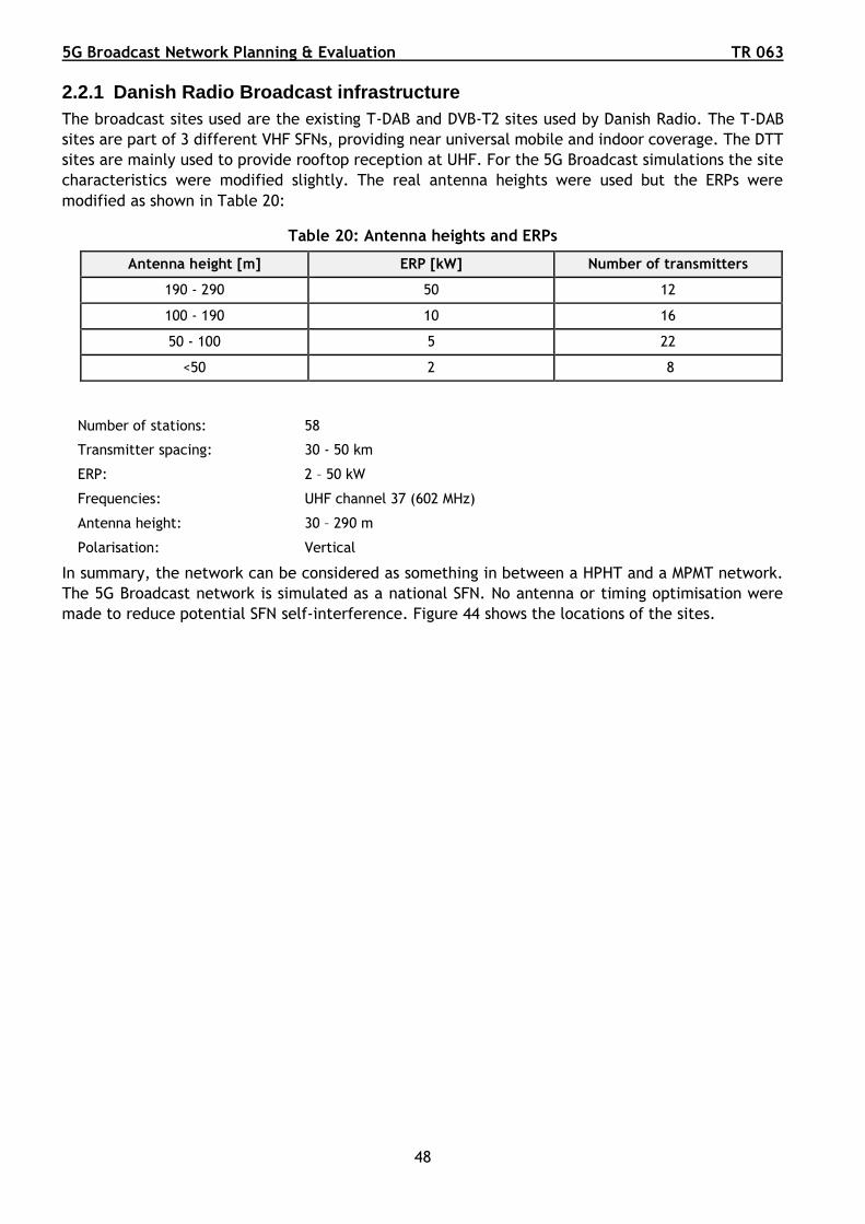
5G Broadcast Network Planning & Evaluation TR 063
48
2.2.1 Danish Radio Broadcast infrastructure
The broadcast sites used are the existing T-DAB and DVB-T2 sites used by Danish Radio. The T-DAB
sites are part of 3 different VHF SFNs, providing near universal mobile and indoor coverage. The DTT
sites are mainly used to provide rooftop reception at UHF. For the 5G Broadcast simulations the site
characteristics were modified slightly. The real antenna heights were used but the ERPs were
modified as shown in Table 20:
Table 20: Antenna heights and ERPs
Antenna height [m] ERP [kW] Number of transmitters
190 - 290 50 12
100 - 190 10 16
50 - 100 5 22
<50 2 8
Number of stations: 58
Transmitter spacing: 30 - 50 km
ERP: 2 – 50 kW
Frequencies: UHF channel 37 (602 MHz)
Antenna height: 30 – 290 m
Polarisation: Vertical
In summary, the network can be considered as something in between a HPHT and a MPMT network.
The 5G Broadcast network is simulated as a national SFN. No antenna or timing optimisation were
made to reduce potential SFN self-interference. Figure 44 shows the locations of the sites.

TR 063 5G Broadcast Network Planning & Evaluation
49
Figure 44: The Danish DAB sites used in the study (58 sites in total)
2.2.2 5G transmission modes and planning parameters
Several different 5G transmission modes were simulated. They represented a range from very robust
modes using QPSK, requiring low C/(N+I) values and providing little capacity, to modes using
256-QAM, requiring high C/(N+I) values and providing capacity equivalent to DVB-T2 transmissions
used today. As there is currently some uncertainty regarding the capacity achieved for a certain C/N
for 5G Broadcast, the results are presented as population covered for available C/(N+I), from 0 to
25 dB in steps of 5 dB, i.e., for 0, 5, 10, 15 ,20 and 25 dB. It is, however, easy to translate the results
to capacity when consolidated mappings from C/N to capacity are available for the different
reception cases.
The CP has been set to 200 µs and 300 µs to evaluate the influence of using different CP values.
The bandwidth (BW) of the 5G Broadcast signal is set to 5 MHz, to align with the Monte Carlo
simulations in the previous sections.
The planning parameters agree with § A1 (Annex A), i.e., the same parameters as in the Monte Carlo
simulations are used. Some of these parameters are presented below. The reception scenarios that
are considered in the study are highlighted in Table 21. These are Car Mounted mobile reception,
Handheld Portable Outdoor reception and Handheld Portable Indoor reception.

5G Broadcast Network Planning & Evaluation TR 063
50
Table 21: Planning parameters used in the coverage simulations
Scenarios
Car
mounted
(CM)
Handheld
In Car
Handheld
portable
outdoor
Fixed
rooftop
Portable
indoor
Handheld
portable
indoor
Type of reception Mobile Mobile HH
Portable Fixed Portable
HH
Portable
Receiver antenna gain, (dBi) 3 8.3 8.3 13 4.3 8.3
Receiver diversity gain 0 2.5 2.5 0 6 2.5
Entry loss (dB) –
Building/vehicle 0 9 0 0 11 11
Standard deviation of
Building Entry loss (dB) 0 5 0 0 6 6
Receiver height (m) 1.5 1.5 1.5 10 1.5 1.5
Receiver feeder loss (dB) 0 0 0 4 0 0
Other losses (dB) 1 1 1 1 1 1
Receiver Noise Figure (dB) 6 9 9 6 9 9
Required Location
Percentage 95% 95% 95% 95% 95% 95%
When assessing coverage, the possible impact of the CAS (Cell Acquisition Subframe) in 5G Broadcast
was not considered. To allow the receiver to correctly interpret the Broadcast content, the CAS in
5G Broadcast needs to be received and decoded. The CAS should in theory be very robust, but there
is currently some uncertainty regarding how well the CAS will perform in real cases.
2.2.3 Planning software and databases
To assess coverage the PROGIRA® software20 was used. 5G Broadcast coverage was simulated using a
dedicated 5G Broadcast module. The field strength predictions were made using the CRC Predict
terrain-based propagation model. The propagation model was tuned to the clutter and height data
in Denmark using field measurement data. Mean error is near 0 dB with a spread (standard deviation)
between 5 and 7 dB around UHF 600 MHz. The following geographical databases were used:
• Terrain Elevation data (25 m).
• Clutter data (50 m), which includes 5 different classes representing built areas (dense urban,
urban, suburban, residential, and industrial).
• Population data (100 m).
The wanted field strength has been calculated using 50% of time propagation and the interfering field
strength with 1.7% of time (to assess potential SFN self-interference).
20 https://www.progira.com/spectrum-planning-software/

TR 063 5G Broadcast Network Planning & Evaluation
51
2.2.4 Results for 200 µs Cyclic Prefix
To start with the C/(N+I) (SINR) for the network was calculated.
Figure 45: Median (50% of locations) Raw achievable C(N+I) mobile
From the map in Figure 45, it seems that it is possible to achieve a C/(N+I) above 20 dB in a large
part of the country. It should however be kept in mind that this is the median C/(N+I), valid for 50%
of locations. For broadcast services we normally use a target service probability of 95% of locations
or even 99% for mobile reception. Additionally, we need to be able to evaluate the impact of possible
SFN self-interference in the network, which may occur if the Cyclic Prefix is not long enough. This is
particularly important for the less robust modulation and code rate (MCS) in 5G Broadcast, where
SFN self-interference can be substantial.
SFN simulations for the different required C/(N+I) are presented in Table 22 (CP 200 µs).

5G Broadcast Network Planning & Evaluation TR 063
52
Table 22: Population coverage for 95% of locations for CP of 200 µs
C/N Req [dB] Mobile
Car Mounted
Population (No SFN self-interference)
[% of total pop] 95% locations
Population (With SFN self-interference)
[% of total pop] 95% locations
0 99.2 92.4
5 98.9 82.7
10 97.7 64.9
15 94.1 42.1
20 86.5 22.1
25 82.6 10.2
Table 22 shows that the coverage, when not considering SFN self-interference, is quite good. The
network can provide coverage to 94% of population at 15 dB C/N+I. But when SFN self-interference
is considered, the coverage drops significantly. Figure 46 illustrates the difference in surface
coverage between two C/N+I thresholds, taking SFN self-interference into consideration
Figure 46: Mobile Car mounted coverage, C/(N+I) of 20 dB (left) and 10 dB (right)
at 95% of locations for CP of 200 µs.
The main limitation at higher required C/N values is SFN self-interference. From this the conclusion
to be drawn is that it might be difficult to use a MCS which requires a higher C/N than, say, 5 dB,
resulting in very limited capacity for mobile Car Mounted reception. It should, however, be borne in
mind that the case of a national SFN in Denmark is a critical case. The country is very flat and there
are sea paths between the different Islands, which results in high field strengths for 1.7% of time. In
the example no further attempts to optimize transmitter timing and antenna directions to reduce
SFN self-Interference were made. Such an optimisation would of course improve coverage, but due
to the large impact it would not be realistic to implement such a large SFN using a CP of 200 µs.
Summarizing the results for all three reception cases for 200 µs CP are Table 23 and Figure 47.

TR 063 5G Broadcast Network Planning & Evaluation
53
Table 23: population coverage for Car mounted, Handheld Indoor
and Handheld Outdoor reception using a CP of 200 µs
C/N Handheld Indoor % Car Mounted % Handheld Outdoor %
0 dB 82.7 92.4 92.5
5 dB 71.5 82.7 82.7
10 dB 47.5 64.9 64.9
15 dB 22.7 42.1 41.6
20 dB 7.8 22.1 21.3
25 dB 2.6 10.2 9.3
Figure 47: Graphical results for CP of 200 µs
We can conclude that for Handheld Indoor reception, coverage is mainly limited by lack of field
strength. For Car Mounted and Handheld Outdoor coverage it is limited mainly by SFN
self-interference, in particular at higher required C/(N+I ). Moreover, a CP of 200 µs is not long
enough to work in larger SFNs using high power broadcast sites.
2.2.5 Results for a cyclic prefix of 300 µs
If we do the calculation using a CP of 300 µs. We will see a significant improvement in SFN coverage.
In the case of Mobile Car Mounted reception we get the results shown in Table 24.

5G Broadcast Network Planning & Evaluation TR 063
54
Table 24: Population coverage for 95% of locations for CP of 300 µs.
C/N Req [dB] Mobile
Car Mounted
Population (No SFN self-interference)
[% of total pop] 95% locations
Population (With SFN self-interference)
[% of total pop] 95% locations
0 99.3 99.3
5 99.3 99.3
10 99.3 99.3
15 99.3 99.2
20 99.1 98.3
25 98.2 92.9
Figure 48: Mobile Car mounted coverage, C/(N+I) of 15 dB (left) and 25 dB (right)
at 95% of locations for CP of 300 µs.
The “only” difficulty with using a CP of 300 µs is the sensitivity to Doppler. According to § 1.7.2,
limitation due to Doppler would not allow the use of 5G Broadcast modes to vehicles travelling faster
than 106 km/h if the required C/N exceeds 10 dB.
If we summarize the results for all three reception modes, we see (Table 25 and Figure 49) that the
network would also provide very good coverage for Handheld Indoor reception.
For a required C/N of 10 dB it could serve 92% of the population.
Table 25: Population coverage for Car Mounted, Handheld Indoor
and Handheld Outdoor reception using a CP of 300 µs
C/N Handheld Indoor % Car Mounted % Handheld Outdoor %
0 dB 99 99.3 99.3
5 dB 97.9 99.3 99.3
10 dB 92.1 99.3 99

TR 063 5G Broadcast Network Planning & Evaluation
55
15 dB 70.6 99.2 97.3
20 dB 37.6 98.3 90.1
25 dB 15.8 92.9 66.6
Figure 49: Graphical results for 300 µs CP
We see that Handheld Indoor reception at high C/N is difficult due to the lack of field strength when
considering building entry loss. Handheld Outdoor and Car Mounted reception is very good but of
course suffers from the receiver speed limitation due to Doppler for Car Mounted reception.
2.2.6 Adding LPLT transmitter in regional SFN
From the earlier simulations we can conclude that a CP of 300 µs will have limitations due to Doppler
performance and a CP of 200 µs will provide limited coverage in an SFN. For this reason, a few
calculations were also made in a regional SFN, where SFN self-interference has little or no impact
when using a CP of 200 µs.
The study was made using the Danish island of Zealand with a size of about 100 km x 100 km and a
total population of about 2 million, largely concentrated in the capital city Copenhagen. See
Figure 50.

5G Broadcast Network Planning & Evaluation TR 063
56
Figure 50: Broadcast Network on the island of Zealand
The existing broadcast infrastructure on Zealand consist of 10 sites, 3 high power sites and 7 medium
power sites. As we knew from the earlier work that Handheld Outdoor and Car Mounted reception
will be quite good if SFN self-interference can be avoided, we performed the calculations to
investigate Handheld Indoor reception. The requirements are as follows:
• Handheld Indoor Service
• C/N 20 dB
• Coverage criteria is 95% of locations
• Cyclic Prefix 200 µs
• Population coverage target is 95% of population
From previous experience we knew that it will be difficult for a broadcast infrastructure to provide
Handheld Indoor. To complement the broadcast network, we have “access” to about 900 LTE 700 MHz
base stations. Positions are taken from the official site database and whilst antenna heights are not
given, we assumed an antenna height of 30 m and an EIRP of 700 W.

TR 063 5G Broadcast Network Planning & Evaluation
57
Figure 51: Handheld indoor coverage using only Broadcast network (left) and Broadcast
network complemented by 425 Telecom sites (right) to reach the population target of 95%
The broadcast network alone achieves a Handheld Indoor reception of 24% (left map in Figure 51).
About 425 additional Telecom sites are needed to reach the 95% population target (right map in
Figure 51).
If we now “remove” the broadcast network completely and “rely” only on the 425 telecom sites
population coverage will drop to 78%. To again reach the 95% population target there is a need to
add about 200 Telecom sites to “replace” the Broadcast network.

5G Broadcast Network Planning & Evaluation TR 063
58
Figure 52: Handheld Indoor coverage using only 425 Telecom sites (left) and when adding 195
to a total of 620 Telecom sites (right) to reach the population target of 95%
In the left map of Figure 52 it can be seen where the Broadcast sites are missing.
Even if the original Handheld Indoor coverage by the broadcast network alone (24%) is low, it still
provides quite good “umbrella” coverage in the SFN and almost 200 Telecom sites are needed to
replace them.
The results are summarized in Table 26.
Table 26: Summary of results for the regional SFN
Network type Number of
Broadcast sites
Number of
Telecom sites
Population coverage
HH indoor 95% locations
Broadcast Only 10 - 24%
Broadcast and Telecom 10 425 95%
Telecom (Broadcast removed) - 425 78%
Telecom Only - 620 95%
2.2.7 Conclusions
In the study we have simulated LTE based 5G Broadcast coverage for a network based on existing
Broadcast infrastructure. The following conclusions may be drawn:
In a large area SFN in flat area with sea paths:
• The Cyclic Prefix of 200 µs is too short. There will be significant limitations due to SFN
self-interference
• SFN self-interference is reduced significantly when using a CP of 300 µs. Even system variants
requiring a C/N of 20 dB would provide population coverage above 90% for Handheld Outdoor and
Car Mounted reception.
• Car Mounted reception using 300 µs CP will be difficult above, say, 100 km/h due to Doppler for
system variants which require a C/N above 10 dB
In Regional SFNs:
• Use of 200 µs CP would provide good Handheld Outdoor and Car Mounted reception at C/N of up
to 20 dB
• Broadcast networks alone will not provide coverage at high C/N for Handheld Indoor reception
• When combining Broadcast (HP and MP) infrastructure with Telecom sites, broadcast sites may
be used to provide significant umbrella coverage in an SFN

TR 063 5G Broadcast Network Planning & Evaluation
59
3. Overall conclusions
The simulations carried out on theoretical networks as well as those based on real networks in Italy
and Denmark (two quite different countries in terms of size and terrain morphology) allow the
following conclusions to be drawn:
• Homogeneous21 HPHT or MPMT22 networks show good performance for Fixed Roof Top reception,
with a relatively low density of transmitters, but have limitations in terms of coverage and
available SINR for Car Mounted reception and significant limitations for Handheld Portable
reception of 5G Broadcast. In SFN mode, full rural area coverage with HPHT for Car Mounted
reception would be possible with SINR of up to 10 dB while MPMT could offer full rural area
coverage for Car Mounted reception with up to 15 dB SINR. However, these values would require
the use of long CP, preferably 300 µs, which is associated with a long symbol time that limits the
maximum achievable speed in Car-Mounted reception due to Doppler effects.
• Homogeneous LPLT networks show good performance for Car Mounted, Handheld Portable and
Fixed reception. They can offer full area coverage for Car Mounted reception in urban and
suburban environments with up to 25 dB SINR and coverage in the same environments for portable
outdoor reception with up to 15 dB SINR. They also work with a lower CP of 100 µs, which is
associated with a short symbol time that allows reception at high speeds. However, to achieve
such coverage and permit use of the lowest cyclic prefix, they require a high site density.
• Hybrid networks, a mix of HPHT/MPMT/LPLT sites, present the best compromise between
performance for Car Mounted and Handheld Portable reception modes in all environments (Rural,
Suburban and Urban) and the number of sites required for a given coverage.
Simulations on theoretical hybrid HPHT/MPMT networks show that full rural area coverage for Car
Mounted reception with SINR of 15 dB in 5 MHz can be obtained with a site density of around 22 sites
per 10000 km2.
In urban and suburban areas, additional MPMT or LPLT sites will be needed. According to simulations
on LPLT networks in urban and suburban areas, full area coverage for Car Mounted and Handheld
Portable outdoor reception with SINR of up to 25 dB in 5 MHz can be obtained with 3 km inter-site
distance. Such inter-site distance corresponds to a site density of 1284 sites per 10000 km2. However,
from the two real case studies described in this report, it may be deduced that an optimized selection
of all site types can significantly reduce the required site density, compared to full LPLT network,
particularly by basing the selection of LPLT sites on high population density areas and main
transportation routes.
The choice of the CP acts on two issues in an opposing manner. On one side a shorter CP, say 100 µs,
helps to achieve higher speed in mobile reception but does not allow mitigation of self-interference
inside large SFNs using HPHT sites. On the other hand, a larger CP, such as 300 µs significantly
mitigates the self-interference in large SFNs of HPHT sites but restricts the speed in mobile reception,
due to the Doppler effect.
Simulations on theoretical networks showed that a CP of 200 µs would be a suitable compromise
between coverage and mobility. This CP allows mobile reception at 600 MHz with a maximum speed
21 Homogeneous means that only one type of site is used in the network. 22 HPHT: High Power High Tower networks.
MPMT: Medium Power Medium Tower networks.
LPLT: Low Power Low Tower networks.
The characteristics of these networks are defined in Annex A.

5G Broadcast Network Planning & Evaluation TR 063
60
of up to around 200 km/h for a SINR of 15 dB. While this CP is largely sufficient for LPLT networks
(which can work even with 100 µs CP), the simulations showed that a CP of 200 µs allows high
coverage rates for Hybrid HPHT and MPMT networks in rural areas for mobile reception with a SINR
of 15 dB with suitable EIRP adjustments.
The real case study in Italy showed that a Hybrid HPHT/LPLT network can give good coverage for
mobile reception with a SINR of 15 dB using a CP of 200 µs with the necessary network optimisation
to reduce the self-interference in the SFN.
The second real case study, on Denmark, showed that 200 µs CP is suitable for a Hybrid
HPHT/MPMT/LPLT Single Frequency Network covering a region of about 100 km x 100 km for
Handheld Indoor reception and Car-Mounted reception at a SINR of up to 20 dB. However, for a
national SFN composed of a mixture of HPHT and MPMT sites aiming at offering a SINR of up to 20 dB
for Car-Mounted and up to 10 dB for Handheld indoor reception, it showed that a 300 µs CP would be
needed to sufficiently mitigate the SFN self-interference.
Regardless of the network configuration, the simulation on theoretical networks showed that it is not
possible to operate SFNs using the same frequency in two contiguous regions or countries with
different editorial contents while providing contiguous coverage across the borders. In these border
areas full coverage requires the use of MFNs. The studies showed that planning MFNs using clusters
of SFNs with frequency reuse 3 or 4 achieves the required coverage. This configuration combines the
benefits of SFN network gain with a sufficiently large co channel separation distance.
In terms of achievable bitrates for 5G Broadcast in Car-Mounted mobile and Handheld Portable
reception, analysis of from the results of the studies described in this report shows that up to 7 Mbit/s
in 5 MHz could be achieved with a SINR of 15 dB and a 200 µs CP.
In carrying out these studies, several questions have arisen that will need to be answered as part of
further work. The studies are based on standard broadcaster assumptions. These include height loss
and standard deviation associated with location variation and the effect of polarisation of the
transmission antenna with respect to the receiving system. These could have a significant impact on
predicted coverage. Given there is divergent information available on the appropriate values to use,
the validity of applying these standard broadcaster assumptions to any studies aimed at assessing
coverage to mobile and handheld devices needs to be investigated.
Verification of these assumptions plus the results of ongoing and future trials of 5G Broadcast
networks will help to confirm the current conclusions.
Future studies should consider enhancement techniques for mobile reception, such as
time-interleaving. It would be also worth investigating closed SFNs23 using the same frequency across
border areas to mitigate the need for MFNs.
23 A Closed SFN uses directional antenna patterns at transmitters located at its edge, oriented towards the centre of the
SFN, to reduce the outgoing interference to neighbouring co-channel networks.

TR 063 5G Broadcast Network Planning & Evaluation
61
4. References / Bibliography
[1] EBU TR 064. Report on Compatibility between 5G Broadcast and other DTT systems in the
sub-700 MHz band, July 2021.
[2] EBU Tech 3348. Frequency and network planning aspects of DVB-T2
[3] EBU S-SPT Docs 377, 378 and 379 eMBMS simulator description
[4] 5G X cast Deliverable D3.1 LTE--Advanced Pro Broadcast Radio Access Network Benchmark
v1.1, 29/06/2018
[5] 3GPP TS 36.214, v14.0.0, 2016--09, ‘Technical Specification Group Radio Access Network;
E--UTRA;Physical Layer; Measurements Release 14
[6] Monte Carlo based time variation of signals in broadcast network simulations – Simon Elliott
& David Vargas (BBC), Jordi Giménez (IRT), Assunta De Vita (RAI), Alberto Rico-Alvariño &
Amer Catovic (Qualcomm Inc.), Richard Rudd (Plum Consulting/ITU SG3), Erik Stare
(Ericsson) - EBU Technical Review February 2020.
[7] Receiving Antenna Alignment in Hexagonal Grid Simulations - Simon Elliott (BBC), Jordi
Joan Gimenez (IRT), Assunta De Vita (RAI), David Vargas (BBC) – A Study for LTE-based 5G
Terrestrial Broadcast - EBU Technical Review February 2020.
[8] ‘Redundancy on Demand – Extending the Coverage Area of Terrestrial Broadcast via
Broadband Networks’, J. Qi, J. Zollner, J. Robert, L. Stadelmeier and N. Loghin, IEEE
Transactions on Broadcasting, Vol. 60, No.2, June 2014.
[9] ‘Field Trial of a Redundancy on Demand DVB-T2 System’, F. Schreiber, J. Zollner, L.
Stadelmeier, R. Burow, F. Kattanek, S. Krueger, IEEE 2016.
[10] OFDM Receivers – impact on coverage of inter--symbol interference and FFT window
positioning, R. Brugger (IRT), D. Hemingway (BBC), EBU Tech Review 295, 30 July 2003
[11] ITU Document 6A/198 - Liaison statement to Working Party 6A - Report on the work of
Correspondence Group 3K-4 concerning the correlation of short term interfering signals,
11 March 2013
[12] TG6(14)070Rev2, ‘The relationship between ISD and SINR in LTE eMBMS networks for fixed
rooftop reception’, 13 May 2014
[13] EBU S-SPT Document 413 – 5G-Broadcast LPLT sites
[14] Performance of 5G Broadcast and benefits of proposed time--interleaving enhancements,
David Vargas, Simon Elliott, Oliver Haffenden, Ryan McCartney, Andrew Murphy (all BBC),
Jordi Joan Jimenez (5G MAG) – IBC Technical Paper, 14 September 2020.
[15] LTE; Evolved Universal Terrestrial Radio Access (E-UTRA); Physical Layer procedures - 3GPP
TS 36.213 version 16.3.0 Release 16 / ETSI TS 136 213 V16.3.0 (2020-11)
[16] Equalization of FFT-leakage in mobile DVB-T. Master Thesis in Radiocommunication from
the Royal Institute of Technology, Stockholm performed at TERACOM AB, Stockholm,
Sweden by Guillaume Geslin - April 1998.

5G Broadcast Network Planning & Evaluation TR 063
62

TR 063 5G Broadcast Network Planning & Evaluation
63
Annex A: Simulation parameters for 5G Broadcast generic
network simulations
Where applicable, the following parameters are defined for a working frequency centred on 600 MHz.
A1. Time percentage of signals
Where only location variation is considered, wanted signals are predicted using 50% of time curves
from Recommendation ITU-R P.1546-5; unwanted signals are predicted using 1.75% of time curves,
to account for a simplified model for correlation between interfering signals as advised by ITU-R
WP6A in document 6A/198 / Simple method.
In the case of location and time variation simulations, wanted and unwanted signals are predicted
using a time varying propagation model (Recommendation ITU-R P.1546-5 extended beyond its
[1-50]% validity domain to [0-100]% of time by extrapolation), with a target availability of 99% of
time.
A2. 5G Broadcast system parameters
Table A1 describes the valid combination of system parameters for 5G Broadcast data signals: CAS
signalling can only use variant 1, while the useful payload (carried by the PMCH – Physical Multicast
Channel) may adopt any variant from 2 to 6. Those parameters were derived from 3GPP TS36.211
v16.1.0 (2020-03) “E-UTRA Physical channels and modulation (Release 16)”.
Table A1: 5G Broadcast system parameters
Variant
Carrier
Spacing
delta f
[kHz]
Subcarriers
/ RB
OFDM symbols /
subframe
Tu
(µs)
#Tu
samples
CP
(µs)
#CP
samples
Ts
(µs)
CP
Ratio Dx Dy
Nyquist
factor
Nyquist
limit
(µs)
EI- Equalisat
ion interval
/ Tp24 (µs)
1 15.00 12 14 66.7 2044 4.7 144 71.40 5/71 3 5 1/3 22.23 19.80
2 15.00 12 12 66.7 2045 16.7 512 83.40 1/4 1 4 1 66.70 59.40
3 7.50 24 6 133.3 4099 33.3 1024 166.60 1/4 2 2 1/2 66.65 59.36
4 1.25 144 1 800 24576 200 6144 1000.00 1/4 3 1 1/3 266.67 237.50
5 2.50 72 2 400 12288 100 3072 500.00 1/4 2 1 1/2 200.00 178.13
6 0.37 486 1 2700 82944 300 9216 3000.00 1/9 3 1 1/3 900.00 801.56
Note: in COFDM based broadcasting systems with fixed bandwidth, an FFT size is specified. In 5G
Broadcast system, as the channel width can vary, no FFT size is specified, but rather a carrier spacing:
100 µs CP → 2.5 kHz carrier spacing
200 µs CP →1.25 kHz carrier spacing
300 µs CP →0.37 kHz carrier spacing
24 Equalization interval duration is usually taken as 57/64 of the Nyquist limit to reflect real implementation of receivers.

5G Broadcast Network Planning & Evaluation TR 063
64
As a comparison, if we consider a 5 MHz channel in 5G Broadcast, with 25 Resource Blocks (180 kHz
/ RB), the above figures would correspond to 2K / 4K / 13.5K FFT respectively.
A3. Reception parameters
Table A2 deals with the reception parameters used in the simulations for each of the agreed
scenarios, with the following additional assumptions:
The receiver and transmitters are assumed to use the same polarization; hence no polarization
discrimination is assumed.
The receiver and the transmitter are considered as being in the same environment; the receiver
clutter height depends on the environment as follows:
Clutter height = 10 m for a Rural or Suburban environment
Clutter height = 20 m for an Urban environment
Clutter height = 30 m for a Dense Urban environment (only for reference, not considered in the
simulations)
Table A2: Reception parameters used in the simulations for each of the agreed scenarios
Scenarios 1 2 3 4 5 6
Reception parameters
Car
mounted
(CM)
Handheld
In-Car
Handheld
portable
outdoor
Fixed rooftop
(FRT)
Portable
indoor
(PI)
Handheld portable
indoor
(P-H/Internal
Antenna)
Type of reception Mobile Mobile Portable Fixed Portable Portable
Path type Land Land Land Land Land Land
Receiver antenna gain, including
possible body loss and receiver
diversity gain (dBi)
3 -5.8 -5.8 13 1.7 -5.8
Entry loss (dB) – Building/vehicle 0 9 0 0 11 11
Standard deviation associated
with entry loss (dB) 0 5 0 0 6 6
Receiver height (m)25 1.5 1.5 1.5 10 1.5 1.5
Receiver feeder loss (dB) 0 0 0 4 0 0
Other losses26 (dB) 1 1 1 1 1 1
Receiver strategy for signals from
the same SFN Maximum C/I
Location variation standard
deviation (dB) 5.5
Receiver Noise Figure (dB) 6 9 9 6 9 9
25 Received field strength is predicted using the ITU-R Recommendation P.1546-5 model at the specified receiver height,
considering the receiver clutter height corresponding to the receiver environment (rural, suburban, urban). At 600 MHz,
for rural environment, this corresponds to a height loss of 16.8 dB, for suburban environment to a height loss of 17 dB and
for urban environment to a height loss of 23.3 dB for a 1.5 m reception height when compared to the reception at the
height of the representative receiver clutter height of the corresponding environment.
26 Other losses account for implementation losses (front-end performances). There could be other losses related to the
performance of the transmitter, like Error Vector Magnitude for LPLT transmitters, but these are not considered in this
study.

TR 063 5G Broadcast Network Planning & Evaluation
65
Percentage of locations to protect
on a small area27 95% 95% 95% 95% 95% 95%
A4. Transmission parameters
Three network types were agreed for the modelling of 5G Broadcast networks:
Network type 1: High Power High Tower (HPHT)
Network type 2: Medium Power Medium Tower (MPMT)
Network type 3: Full cellular / Low Power Low Tower (LPLT)
Note: antenna polarization has no incidence on simulation as both the transmitter and receiver are
assumed to use the same polarization. This parameter is not described in the following paragraphs.
As the parameters for modelling the HPHT and MPMT networks are taken from real-life broadcast
deployments, all the EIRP values reported in the following paragraphs are referenced by convention
to an 8 MHz bandwidth (7.77 MHz effective channel). To use those EIRP values for a precise 3GPP
bandwidth, a specific correction factor must be applied as described in § A4.5.
A4.1 Network type 1 parameters - HPHT
Table A3 describes the parameters used for the modelling of HPHT networks. Annex B provides useful
analysis of inter-site distance of HPHT networks in Sweden, France and the United Kingdom
Table A3: Parameters used for the modelling of HPHT networks
Network type HPHT
Inter-Site Distance (km) – ISD 50, 60, 70, 80, 100, 120
EIRP (dBm) 76, 79, 82, 8528
Antenna height above ground level (m) 200, 300, 350
Tilt (° positive below horizontal) 1, 2, 3°29
Environment type Rural
Clutter height (m) 10
A4.2 Network type 2 parameters - MPMT
Table A4: Parameters used for the modelling of MPMT networks
Network type MPMT
Inter-Site Distance (km) – ISD 20, 30, 40, 50
EIRP (dBm) 62, 69, 7230
Antenna height above ground level (m) 80
27 For mobile and portable reception, the percentage of locations to protect on a small area can also include 70%, 90% and
99%; for fixed reception, 90% can also be considered.
28 Corresponding to 25 kW, 50 kW and 100 kW ERP respectively. 29 Vertical antenna pattern according to ITU-R BT.2337 High Power for DVB-T/DVB-T2.
30 Corresponding to 1 kW, 5 kW and 10 kW ERP respectively.

5G Broadcast Network Planning & Evaluation TR 063
66
Tilt (° positive below horizontal) 0°31
Environment type Rural
Clutter height (m) 10
A4.3 Network type 3 parameters – LPLT
Report ITU-R M.2292 has been used as the source to identify Low Power Low Tower network
parameters (shown in Table A5).
Table A5: Parameters used for the modelling of LPLT networks – M.2292
Network type Full cellular - LPLT
Environment type Rural Suburban Urban
Inter-Site Distance (km) – ISD32 12 3 3
EIRP (dBm)33 57.4 / 59.4 57.4 / 59.4 57.4 / 59.4
Antenna height above ground level (m) 30 30 30
Tilt (° positive below horizontal) 3°34
Clutter height (m) 10 10 20
A4.4 Reference vertical radiation patterns
The following figure illustrates the resulting vertical radiation patterns considered in the simulations
according to the selected parameters.
Note: the MPMT vertical radiation pattern is given for reference only, as for MPMT no vertical
radiation pattern is considered.
31 No vertical antenna pattern.
32 Calculated from a specified cell radius > 5 km (8 km typical) for macro rural scenario and 0.5 - 5 km (2 km typical) for
macro urban/suburban scenario.
33 57.4 dBm corresponds to approximately 550 W EIRP. This value is derived from Base station EIRP/sector of 58 dBm in
10 MHz, with 0.6 dB reduction for the 8/10 MHz ratio. A 3 dB reduction is specified in ITU-R M.2292 to take account of an
average base station activity factor of 50%; this reduction is not applied in the case of 5G Broadcast as the system is always
active.
34 Recommendation ITU-R F.1336 (equation 1d) with 9.1 degrees 3 dB beamwidth in the elevation plane and k = 0.3.

TR 063 5G Broadcast Network Planning & Evaluation
67
Figure A1: Vertical radiation patterns for the different types of networks (without tilt)
A4.5 Correction factor with respect to the channel bandwidth
When considering a different channel bandwidth, and more specifically in the case of 3GPP agreed
system bandwidth, a correction must be applied to the EIRP values to keep the EIRP / MHz constant,
as well as the resulting signal-to-noise ratio (SNR) in case the bandwidth is changed. The
corresponding correction is given in the table below.
Table A6: EIRP correction factor depending on channel bandwidth
Channel BW (MHz) 1.4 3 5 10 15 20
Effective BW (MHz) 1.08 2.7 4.5 9 13.5 18
Correction factor (dB) -8.6 -4.6 -2.4 0.6 2.4 3.6

5G Broadcast Network Planning & Evaluation TR 063
68
Annex B: Inter Site Distance
To better understand the inter-site distance of HPHT networks, an analysis of such sites in Sweden,
France and the United Kingdom was carried out. Given coordinates of sites, the distance to the
nearest neighbours can be derived using Delaunay triangulation.
Care needs to be taken to filter (to remove false, not valid) sides of the generated triangles,
illustrated in Figure B1. In the case of Sweden, with the false sides included, the average ISD for the
57 HPHT sites is 105 km, removing false sides the ISD reduces to 93 km, see Figure B2.
Full Delaunay Triangulation Filtered Delaunay Triangulation
Figure B1: ISD of HPHT Sites in Sweden

TR 063 5G Broadcast Network Planning & Evaluation
69
Figure B2: CDF of HPHT ISD in Sweden
Triangulation for the 112 main French sites with false links at the edge removed, Figure B3,
provides a median ISD value of 82 km, Figure B4. Terrain and population play a part in the
site spacing. Low ISD values can be found in Paris, the Alps and the Jura, high ISD values
around Toulouse Pic-du-Midi (Southeastern France).
Figure B3: ISD of HPHT Sites in France
Figure B4: CDF of HPHT ISD France
Triangulation for the 50 main UK sites with links over 100 km removed provides a median ISD
value of 73 km, see Figure B5.

5G Broadcast Network Planning & Evaluation TR 063
70
Figure B5: CDF of HPHT ISD United Kingdom
Taking the results for Sweden, France and the United Kingdom and recognising that there is a spread
in results and that values for other countries may differ significantly, for generic studies an ISD for
HPHT sites of 80 km could be used.

TR 063 5G Broadcast Network Planning & Evaluation
71
Annex C: Results of coverage simulations at national or regional borders
C1. HPHT results
The scenario is based on a HPHT network topology with the following characteristics:
• Rural reception
• 80 km ISD
• 300 m antenna height
• 2° antenna tilt
• 79.6 dBW EIRP
• 300 µs Cyclic Prefix duration
C1.1 Corner regional boundary results
Original situation (no boundaries)
Corner – 0 ISD
Corner – 1 ISD

5G Broadcast Network Planning & Evaluation TR 063
72
Corner – 2 ISD
The following figure compares the resulting complementary CDF of SINR for the 4 situations presented
above.
Figure C1: Corner regional boundary results for HPHT
C1.2 Straight regional boundary (East/West separation)
Original situation (no boundaries)

TR 063 5G Broadcast Network Planning & Evaluation
73
E/W – 0 ISD
E/W – 1 ISD
E/W – 2 ISD

5G Broadcast Network Planning & Evaluation TR 063
74
Figure C2: Straight E/W boundary region results comparison for HPHT
C1.3 Straight regional boundary results (North/South separation)
Original situation (no boundaries)
N/S – 0 ISD

TR 063 5G Broadcast Network Planning & Evaluation
75
N/S – 1 ISD
N/S – 2 ISD
Figure C3: Straight N/S boundary region results comparison for HPHT
C2. MPMT results
The scenario is based on a MPMT network topology with the following characteristics:
• Rural reception.
• 20 km ISD.

5G Broadcast Network Planning & Evaluation TR 063
76
• 80 m antenna height.
• no antenna tilt (and no vertical pattern).
• 59.6 dBW EIRP.
• 300 µs Cyclic Prefix duration.
C2.1 Corner regional boundary results
Original situation (no boundaries)
Corner – 0 ISD
Corner – 1 ISD

TR 063 5G Broadcast Network Planning & Evaluation
77
Corner – 2 ISD
The following figure compares the resulting complementary CDF of SINR for the 4 situations presented
above.
Figure C4: Corner regional boundary results for MPMT
C2.2 Straight regional boundary (East/West separation)
Original situation (no boundaries)

5G Broadcast Network Planning & Evaluation TR 063
78
E/W – 0 ISD
E/W – 1 ISD
E/W – 2 ISD

TR 063 5G Broadcast Network Planning & Evaluation
79
Figure C5: Straight E/W boundary region results comparison for MPMT
C2.3 Straight regional boundary results (North/South separation)
Original situation (no boundaries)
N/S – 0 ISD

5G Broadcast Network Planning & Evaluation TR 063
80
N/S – 1 ISD
N/S – 2 ISD
Figure C6: Straight N/S boundary region results comparison for MPMT
C3. LPLT results
The scenario is based on a LPLT network topology with the following characteristics:

TR 063 5G Broadcast Network Planning & Evaluation
81
• Rural reception.
• 12 km ISD.
• 30 m antenna height.
• 3° antenna tilt.
• 57 dBW EIRP.
• 100 µs Cyclic Prefix duration.
C3.1 Corner regional boundary results
Original situation (no boundaries)
Corner – 0 ISD
Corner – 1 ISD

5G Broadcast Network Planning & Evaluation TR 063
82
Corner – 2 ISD
The following figure compares the resulting complementary CDF of SINR for the 4 situations presented
above.
Figure C7: Corner regional boundary results for LPLT
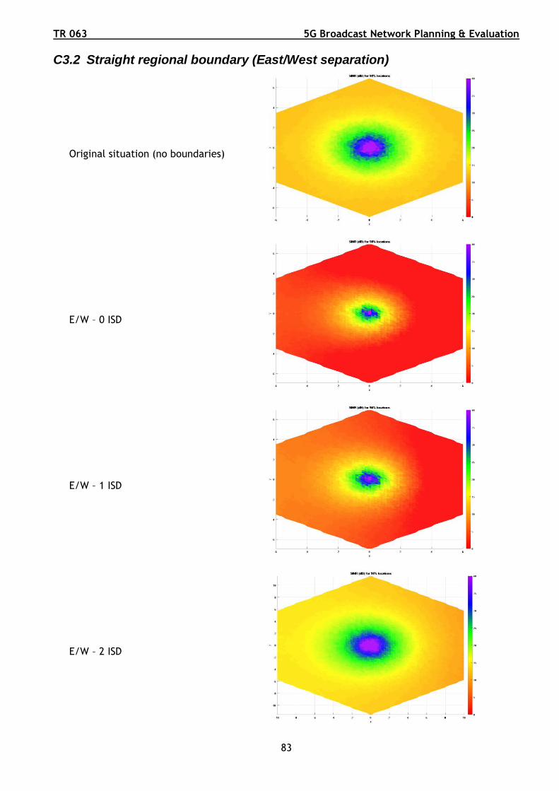
TR 063 5G Broadcast Network Planning & Evaluation
83
C3.2 Straight regional boundary (East/West separation)
Original situation (no boundaries)
E/W – 0 ISD
E/W – 1 ISD
E/W – 2 ISD

5G Broadcast Network Planning & Evaluation TR 063
84
Figure C8: Straight E/W boundary region results comparison for LPLT
C3.3 Straight regional boundary results (North/South separation)
Original situation (no boundaries)
N/S – 0 ISD

TR 063 5G Broadcast Network Planning & Evaluation
85
N/S – 1 ISD
N/S – 2 ISD
Figure C9: Straight N/S boundary region results comparison for LPLT

5G Broadcast Network Planning & Evaluation TR 063
86
Annex D: Capacity versus SINR mapping
Tables D1, D2 & D3 provide an indicative mapping of the 5G Broadcast system capacity with the
corresponding signal-to-Interference-plus-noise-ratio (SINR) in various reception environments, for a
5 MHz channel. They are based on the recent results relative to link-level simulations of different 5G
Broadcast configurations presented in the IBC Paper [14] for the SINR values.
The 5 MHz channel capacity for the different MCS (Modulation and Coding Schemes) configurations
permitted by the 5G Broadcast system were derived from 3GPP TS 36.213 version 16.3.0 Release 16
[15]. As the capacity slightly varies with the number of resource blocks used in the 3GPP system (data
mapping varies with the number of resource blocks, see § 11 of the 3GPP TS 36.213 document), the
corresponding values differ slightly from the IBC Paper, as this last one is based on 10 MHz channels.
In addition, only the information regarding SINR values without possible time-interleaving
enhancements are presented here, as time-interleaving is not a standardized 3GPP feature for the
time being.
Table D1: SNR to capacity mapping for 100 µs CP
MCS
Index MOD COD
Raw
Spectral
Efficiency
(b/s/Hz)
Effective
Spectral
Efficiency
(b/s/Hz)
Capacity
(Mbit/s)
In 5 MHz
channel
Fixed
SINR (dB)
Portable
SINR (dB)
Mobile
SINR (dB)
0 QPSK 0.126 0.252 0.133 0.663
1 QPSK 0.167 0.335 0.176 0.881
2 QPSK 0.203 0.406 0.214 1.069
3 QPSK 0.262 0.524 0.276 1.381
4 QPSK 0.333 0.667 0.351 1.755 3.6 3.8
5 QPSK 0.410 0.821 0.432 2.161 4.6 4.6
6 QPSK 0.481 0.963 0.507 2.535 5.6 5.8
7 QPSK 0.576 1.153 0.607 3.034 7 7.2
8 QPSK 0.647 1.295 0.682 3.409 7.8 8.2
9 QPSK 0.742 1.484 0.782 3.908 9.2 9.6
10 16-QAM 0.371 1.484 0.782 3.908 8.2 8.6
11 16-QAM 0.407 1.627 0.856 4.282 9 9.4
12 16-QAM 0.460 1.840 0.969 4.844 10 10.4
13 16-QAM 0.531 2.124 1.119 5.593 11.2 11.4
14 16-QAM 0.598 2.391 1.259 6.295 12.4 12.8
15 16-QAM 0.669 2.676 1.409 7.043 13.2 13.8
16 16-QAM 0.716 2.865 1.509 7.543 14.2 14.8
17 64-QAM 0.478 2.865 1.509 7.543 14.4 15
18 64-QAM 0.493 2.960 1.558 7.792 15 15.6
19 64-QAM 0.564 3.387 1.783 8.915 16.4 17
20 64-QAM 0.612 3.671 1.933 9.664 17.4 18.6
21 64-QAM 0.659 3.956 2.083 10.413 18.4 19.8

TR 063 5G Broadcast Network Planning & Evaluation
87
22 64-QAM 0.707 4.240 2.232 11.162 19.6 21.2
23 64-QAM 0.776 4.658 2.452 12.262 21.6 25
24 64-QAM 0.836 5.013 2.640 13.198 26.4
25 64-QAM 0.871 5.227 2.752 13.759 28
26 64-QAM 0.942 5.653 2.976 14.882
27 64-QAM 0.978 5.867 3.089 15.444
28 256-QAM 0.733 5.867 3.089 15.444
29 256-QAM 0.760 6.080 3.201 16.006
30 256-QAM 0.813 6.507 3.426 17.129
31 256-QAM 0.849 6.791 3.576 17.878
32 256-QAM 0.919 7.351 3.870 19.352
33 256-QAM 0.954 7.636 4.020 20.101
34 256-QAM 0.990 7.920 4.170 20.849
Table D2: SNR to capacity mapping for 200 µs CP
MCS
Index MOD COD
Raw
Spectral
Efficiency
(b/s/Hz)
Effective
Spectral
Efficiency
(b/s/Hz)
Capacity
(Mbit/s)
In 5 MHz
channel
Fixed
SINR (dB)
Portable
SINR (dB)
Mobile
SINR (dB)
0 QPSK 0.113 0.227 0.133 0.663
1 QPSK 0.151 0.301 0.176 0.881
2 QPSK 0.183 0.365 0.214 1.069
3 QPSK 0.236 0.472 0.276 1.381
4 QPSK 0.300 0.600 0.351 1.755
5 QPSK 0.369 0.739 0.432 2.161 4 4 4.6
6 QPSK 0.433 0.867 0.507 2.535 4.8 5 5.6
7 QPSK 0.519 1.037 0.607 3.034 6 6.2 6.8
8 QPSK 0.583 1.165 0.682 3.409 6.8 7 7.8
9 QPSK 0.668 1.336 0.782 3.908 8 8.2 9
10 16-QAM 0.334 1.336 0.782 3.908 7.8 7.8 8.4
11 16-QAM 0.366 1.464 0.856 4.282 8.4 8.4 9.2
12 16-QAM 0.414 1.656 0.969 4.844 9.2 9.2 10.2
13 16-QAM 0.478 1.912 1.119 5.593 10.4 10.4 11.4
14 16-QAM 0.538 2.152 1.259 6.295 11.6 11.4 13
15 16-QAM 0.602 2.408 1.409 7.043 12.4 12.4 14
16 16-QAM 0.645 2.579 1.509 7.543 13.2 13 15.2
17 64-QAM 0.430 2.579 1.509 7.543 13.8 13.4 15.8
18 64-QAM 0.444 2.664 1.558 7.792 14.4 14.4 17
19 64-QAM 0.508 3.048 1.783 8.915 15.6 15.4 19.6
20 64-QAM 0.551 3.304 1.933 9.664 16.8 16.4 22.8
21 64-QAM 0.593 3.560 2.083 10.413 17.8 17.2
22 64-QAM 0.636 3.816 2.232 11.162 19.4 18.2

5G Broadcast Network Planning & Evaluation TR 063
88
23 64-QAM 0.699 4.192 2.452 12.262 22.8 21.8
24 64-QAM 0.752 4.512 2.640 13.198
25 64-QAM 0.784 4.704 2.752 13.759
26 64-QAM 0.848 5.088 2.976 14.882
27 64-QAM 0.880 5.280 3.089 15.444
28 256-QAM 0.660 5.280 3.089 15.444
29 256-QAM 0.684 5.472 3.201 16.006
30 256-QAM 0.732 5.856 3.426 17.129
31 256-QAM 0.764 6.112 3.576 17.878
32 256-QAM 0.827 6.616 3.870 19.352
33 256-QAM 0.859 6.872 4.020 20.101
34 256-QAM 0.891 7.128 4.170 20.849
Table D3: SNR to capacity mapping for 300 µs CP
MCS
Index MOD COD
Raw
Spectral
Efficiency
(b/s/Hz)
Effective
Spectral
Efficiency
(b/s/Hz)
Capacity
(Mbit/s)
In 5 MHz
channel
Fixed
SINR (dB)
Portable
SINR (dB)
Mobile
SINR (dB)
0 QPSK 0.091 0.182 0.132 0.658
1 QPSK 0.122 0.245 0.177 0.887
2 QPSK 0.145 0.291 0.211 1.053
3 QPSK 0.191 0.383 0.277 1.386
4 QPSK 0.240 0.481 0.348 1.739
5 QPSK 0.301 0.603 0.436 2.181
6 QPSK 0.347 0.695 0.503 2.514 3.6 4
7 QPSK 0.428 0.855 0.619 3.097 4.6 4.8
8 QPSK 0.479 0.959 0.694 3.471 5.2 5.6
9 QPSK 0.548 1.097 0.794 3.970 6 6.4
10 16-QAM 0.582 2.327 0.842 4.212 6.8 7.2
11 16-QAM 0.291 1.164 0.842 4.212
12 16-QAM 0.330 1.319 0.955 4.774
13 16-QAM 0.381 1.526 1.104 5.522 8.6 8.8
14 16-QAM 0.428 1.713 1.240 6.201 9.8 9.8
15 16-QAM 0.480 1.920 1.390 6.950 10.2 10.6
16 16-QAM 0.514 2.058 1.490 7.449 10.8 11
17 64-QAM 0.532 3.190 1.540 7.699 11.6 11.8
18 64-QAM 0.615 3.687 1.779 8.897 12.8 13
19 64-QAM 0.658 3.946 1.904 9.521 13.6 13.6
20 64-QAM 0.712 4.270 2.061 10.304 14.6 14.8
21 64-QAM 0.474 2.847 2.061 10.304 15 14.8
22 64-QAM 0.509 3.053 2.211 11.053 15.8 15.6
23 64-QAM 0.567 3.402 2.463 12.314 17.2 16.8

TR 063 5G Broadcast Network Planning & Evaluation
89
24 64-QAM 0.607 3.643 2.637 13.187 18.2 17.8
25 64-QAM 0.634 3.804 2.754 13.770 19 18.2
26 64-QAM 0.679 4.072 2.948 14.739 20.6 19.4
27 64-QAM 0.702 4.210 3.048 15.239 21.4 19.8
28 256-QAM 0.549 4.394 3.181 15.904
29 256-QAM 0.592 4.736 3.429 17.144
30 256-QAM 0.618 4.943 3.579 17.893
31 256-QAM 0.665 5.320 3.852 19.258
32 256-QAM 0.692 5.537 4.008 20.041
33 256-QAM 0.716 5.726 4.145 20.727
34 256-QAM 0.827 6.618 4.791 23.956
The link-level simulations presented in the IBC Paper [14] do not cover all configuration cases and all
reception modes. Moreover, for Fixed reception, they correspond to the use of one antenna, while
for portable / mobile reception two antennas are assumed, leading to diversity gain in the receivers.
As such they provide an upper bound on the capacity associated to a given SINR value.
The values highlighted in green in the tables are the reference SINR values to use when translating a
given SINR value for a given CP to the corresponding capacity, for 5 / 10 / 15 / 20 dB target SINR
respectively. For example, § 1.6 shows that LPLT with reuse 1 offers the best coverage with a 100 µs
CP, ensuring 20 dB in 100% of the target coverage area in suburban or 15 dB in urban area for
Handheld Portable Outdoor reception.
Using the above tables, the indicative available capacity in a 5 MHz channel is 11.162 Mbit/s for
suburban (MCS 22 in Table D2) and 7.792 Mbit/s for urban (MCS 18 in Table D2), if using two different
5 MHz channels, each having its own system characteristics. If the same carrier is to be used for both
urban and suburban coverage, then the lowest MCS index must be selected to allow full coverage in
both urban and suburban areas, hence limiting the capacity to 7.792 Mbit/s in both environments.

5G Broadcast Network Planning & Evaluation TR 063
90
Annex E: Simulation of the Impact of practical antenna pattern
E1. Introduction
This Annex compares the effect on margin and coverage of using an antenna on LPLT, MPMT and
HPHT sites that is subject to practical limitations rather than on ideal antenna characteristics. The
range of antenna variation that exists means it is impractical to model all options, particularly in the
case of LPLT, so a single example has been simulated to show its potential impact. For the LPLT case
the antenna modelled is shown in Figure E6, for the HPHT and MPMT cases a typical ’omnidirectional’
Broadcast antenna incorporating a 4 dB ripple was assessed.
E2. Generic case
The results on coverage of using practical antennas (realisable using existing infrastructure) rather
than idealised antennas are shown in Figures E1 to E5. In all cases there is a reduction in coverage,
however where there is an overlap in coverage and a surfeit of margin for a given SINR, there may
be no real impact on coverage. Examples where coverage for a given SINR is maintained are LPLT
suburban and LPLT urban where SINR is 20 dB or less, LPLT rural where SINR is 5 dB or less, MPMT
and HPHT rural where the SINR is 10 dB or less.
Figure E1 Figure E2

TR 063 5G Broadcast Network Planning & Evaluation
91
Figure E3 Figure E4
Figure E5
E3. ‘Real’ case
The coverage of an example 5G Broadcast network, based on an actual network, was simulated. The
network consists of 130 LPLT sites operated as an SFN. It is designed to provide 95% population indoor
coverage when using idealized antenna diagrams. The details of the modelled network are as follows:
• Extent of area: 30 km x 30 km, approximately 1000 km²
• Environment: Dense Urban 20%, Urban 30% and Suburban 30%
• Type of reception: Handheld Indoor
• Number of sites: 130
• Antenna heights: 20 - 40 m
• Target population coverage: 95%
• EIRP of Sites 500 - 1000 W
• Total population within AOI about 7 million
• Total capacity of network About 10 Mbit/s
SFN system parameters were set in such a way that no SFN self-interference is present, symbol time
is 800 µs and CP is 200 µs. Planning parameters were as specified in Annex A.
The antenna patterns used in the modelling are shown in Figure E6. The difference between the two
idealized and distorted patterns are shown in red.

5G Broadcast Network Planning & Evaluation TR 063
92
Figure E6: Modelled antenna patterns idealized
and distorted
E4. Results
The original network using the ‘idealized’ antenna patterns provided the target 95% indoor population
coverage. Repeating the coverage calculation using the practical antenna pattern provided 73%
indoor population coverage. This indicates that the impact on coverage of a practical antenna pattern
could be significant. It was estimated that about 30 additional sites would be needed to restore 95%
population coverage. Alternatively, an increase of power of about 4 dB would be needed to restore
coverage back to the original 95% population. Coverage plots for the two scenarios modelled are
shown in Figures E7 & E8.
Figure E7: Idealized antenna 95%
indoor population coverage
Figure E8: Practical antenna 73%
indoor population coverage
The difference between the two predictions, i.e., the areas (red) where coverage is lost due to the
change in antenna pattern is shown in Figure E9.

TR 063 5G Broadcast Network Planning & Evaluation
93
Figure E9: Difference plot
E5. Discussion
Broadcast antenna patterns, whilst not providing true omnidirectional coverage, are optimised to
minimise nulls (ripple) in the patterns. Consequently, the impact on SINR at the edge of coverage of
using practical patterns rather than ‘idealised’ omnidirectional patterns is small but not insignificant.
For mobile antenna systems comprised of sector antennas, the impact, if not mitigated, could be
significant at the edge of coverage. The impact on coverage could be reduced by increasing the EIRP,
adopting an increased phase delay between sector antennas (cyclic delay diversity), a combination
of the two or building a new antenna with a better pattern. Each has a cost implication that needs
to be weighed against the potential loss in coverage.
E6. Conclusion
The sector antennas typically used by mobile systems are not designed to operate as arrays. If used
for 5G Broadcast, such antennas would have deep nulls in the pattern, which may compromise
coverage. Measures to mitigate this loss in coverage may be required. Existing broadcast antenna
systems have already been optimised for coverage.