TR/15/85 May 1985

Moment Properties of Estimators For A Type 1 Extreme Value Regression Model

by A.A. Haddow and D.H. Young

z1488297

Moment Properties Of Estimators For A Type 1 Extreme Value Regression Model

by

A. A. Haddow and D .H. Young

Summary

A regression model is considered in which the response variable has a type 1 extreme value distribution for smallest values. Small sample moment properties of estimators of the regression coefficients and scale parameter, based on maximum likelihood, ordinary least squares and best linear unbiased estimation using order statistics for grouped data, are presented, and evaluated, for the case of a single explanatory variable. Variance efficiency results are compared with asymptotic values.

Contents

1 .Introduction

2. Computational Procedures For Maximum Likelihood Estimation

3. Moment Properties Of The Maximum Likelihood Estimators

4. Moment Properties Of The Ordinary Least Squares Estimators

5. Best Linear Unbiased Estimators Based On Order Statistics

For Grouped Data

6. Small Sample Variance Efficiency Results

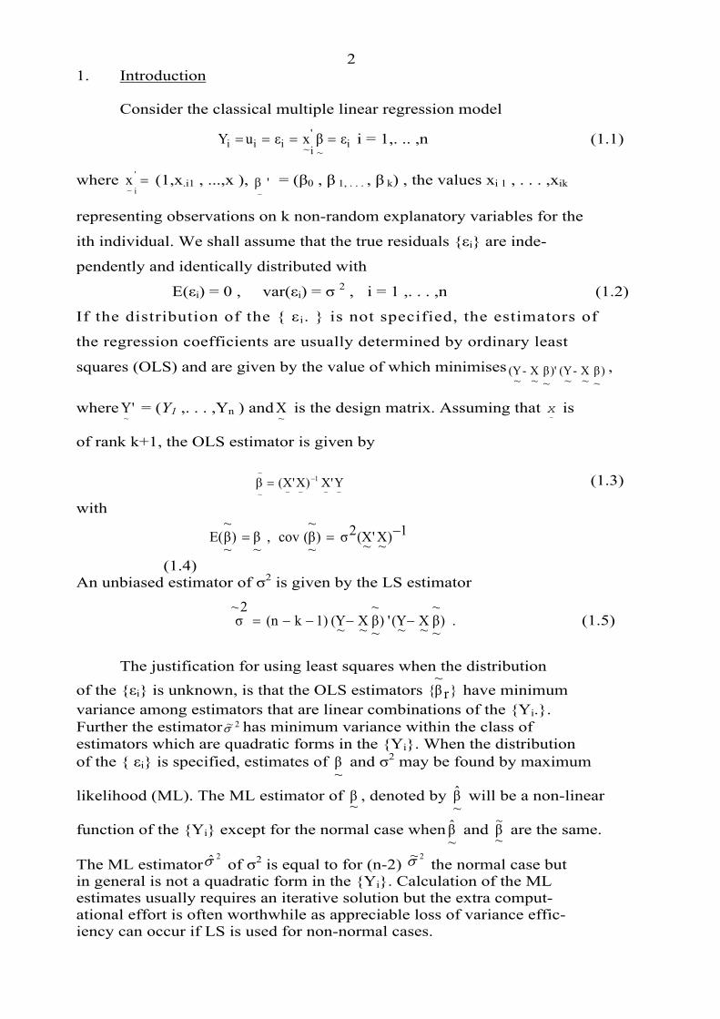
2 1. Introduction

Consider the classical multiple linear regression model

i = 1,. .. ,n (1.1) i~

'i~iii εβxεuY ====

where (1,x='

i~x .i1 , ...,x ), = (β'

~β 0 , β 1, . . . , β k) , the values xi 1 , . . . ,xik

representing observations on k non-random explanatory variables for the

ith individual. We shall assume that the true residuals {εi} are inde-

pendently and identically distributed with

E(εi) = 0 , var(εi) = σ 2 , i = 1 ,. . . ,n (1.2)

If the distribution of the { ε i. } is not specified, the estimators of

the regression coefficients are usually determined by ordinary least

squares (OLS) and are given by the value of which minimises )~β

~X-

~Y()'

~β

~X-

~Y( ,

where = (Y'Y~

1 ,. . . ,Yn ) and is the design matrix. Assuming that is ~X

~x

of rank k+1, the OLS estimator is given by (1.3)

~~

1

~~

~

~Y'X)X'X( −=β

with 1)~X'~X(

2σ)~

~β(cov,

~β)

~

~βE( −==

(1.4) An unbiased estimator of σ2 is given by the LS estimator

.)~

~β~X~Y(' )

~

~β~X~Y(1)k(n

2~σ −−−−= (1.5)

The justification for using least squares when the distribution

of the {εi} is unknown, is that the OLS estimators }r~β{ have minimum

variance among estimators that are linear combinations of the {Yi.}. Further the estimator has minimum variance within the class of 2~σestimators which are quadratic forms in the {Yi}. When the distribution of the { εi} is specified, estimates of and σ

~β 2 may be found by maximum

likelihood (ML). The ML estimator of ~β , denoted by will be a non-linear

~β

function of the {Yi} except for the normal case when and ~β

~β~ are the same.

The ML estimator of σ2σ 2 is equal to for (n-2)

2~σ the normal case but in general is not a quadratic form in the {Yi}. Calculation of the ML estimates usually requires an iterative solution but the extra comput- ational effort is often worthwhile as appreciable loss of variance effic- iency can occur if LS is used for non-normal cases.

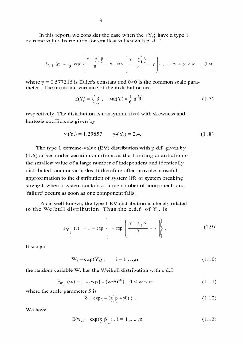
3

In this report, we consider the case when the {Yi} have a type 1 extreme value distribution for smallest values with p. d. f.

(1.6)y,γθ~β'

i~xyexpγθ

~β'

i~xyexpθ

1(y)iYf ∞<<∞−⎪⎭

⎪⎬

⎫

⎪⎩

⎪⎨

⎧

⎟⎟⎟

⎠

⎞

⎜⎜⎜

⎝

⎛

−−

−−−

=

where γ = 0.577216 is Euler's constant and θ>0 is the common scale para- meter . The mean and variance of the distribution are

, ~β'

i~x)iE(Y = 2θ2π61)ivar(Y = (1.7)

respectively. The distribution is nonsymmetrical with skewness and kurtosis coefficients given by

γl(Yi) = 1.29857 γ2(Yi) = 2.4. (1 .8)

The type 1 extreme-value (EV) distribution with p.d.f. given by (1.6) arises under certain conditions as the 1imiting distribution of the smallest value of a large number of independent and identically distributed random variables. It therefore often provides a useful approximation to the distribution of system life or system breaking strength when a system contains a large number of components and 'failure' occurs as soon as one component fails.

As is well-known, the type 1 EV distribution is closely related to the Weibull distribution. Thus the c.d.f. of Yi. is

.γθ~β'

i~xyexpexp1(y)

iYF⎪⎭

⎪⎬

⎫

⎪⎩

⎪⎨

⎧

⎟⎟⎟

⎠

⎞

⎜⎜⎜

⎝

⎛

−−

−−= (1.9)

If we put

Wi = exp(Yi) , i = 1,…,n (1.10)

the random variable W. has the Weibull distribution with c.d.f.

(w) = 1 - exp{ - (w/δ)iwF l/θ} , 0 < w < ∞ (1.11)

where the scale parameter 5 is . (1.12) })x({exp

~

'

i~γθ+β−=δ

We have

i = 1 ,. .. ,n (1.13),)x(exp)w(Ew~

'

i~i β=

4

where

owβ= βo + δθ + logΓ (1+θ) , βwr = βr , r = 1,...,k . (1.14)

It follows that the regression model for the {Yi} with additive model

µi. = ~β'

i~x for the means is equivalent to that based on the {W.} with an

multiplicative exponential model for the means. No special treatment is therefore required for the Weibull model.

When no explanatory variables are present, many investigations have been made to assess and compare the properties of various estimators for the location and scale parameters of the type 1 EV distribution. A useful survey is given by Mann (1968). Lawress (1982) discussed statis- tical inference procedures for the type 1 EV regression model and also gives asymptotic efficiency results for LS estimation relative to ML estimation. However, little work appears to have been done to assess the small sample properties of the estimators in the regression case.

This report focuses attention on the moment properties of estimators for the parameters in the regression model. In section 2, four comput- ational procedures for determining the ML estimators are described and some findings relating to their computational efficiency are given. Approximations to the biases and variances of the ML estimators are given in section 3 and evaluated by simulation for the case of a single explan- atory variable. The OLS estimators are considered in section 4 and in section 5 we discuss the best linear unbiased estimators (BLUE'S) based on order statistics when grouped data are available. Finally, in section 6 small sample variance efficiency results as obtained by simu- lation are compared with asymptotic results.

2. Computational Procedures For Maximum Likelihood Estimation

In this section, we describe four computational methods for determining the maximum likelihood estimates. The first two methods use the Newton- Raphson and Fisher's scoring approach respectively, while the last two methods are designed to facilitate the use of the statistical package GLIM which provides ML fits of generalised linear models.

We first present results for the first and second order derivatives of the logarithm of the density given by (1.6). For notational conven- ience we set

5

i = 1 ,...,n (2.1) ,)xy(z '

i~i1

i γ−−θ= −

and we have

log (yiYf i) = θ-1 exp(zi - ) (2.2) iz

e

with

∂zi/∂β r = -xir /θ , ∂ zi./∂⎝ = -(zi +γ)/θ . We set

θ)i(yiYflog(i)

θU,rβ

)i(yiYflog(i)rU ∂

∂=∂

∂= (2.3)

(2.4)2θ

)i(yiYf log 2(i)θθV,θrβ

)i(yiYf log 2(i)rθV,

sβrβ)i(yiYflog2

(i)rsV

∂

∂=∂∂

∂=∂∂

∂=

for r,s = 0,1,...,k, and a straightforward calculation gives

(2.5) 1} - 1)-izγ)(e+ i{(z1-θ (i)

θ U, 1)- iz(e1- θ ir x= (i)

rU =

γ)}i(zize1- iz

{e2-θirx- (i)rθV , iz

e 2- θ isxir x= (i)rsV ++= (2.6)

(2.7) 1)}-1)- izγ){ei2(ziz

e2γ) i{(z 2- θ - = (i)θθV +++

If L(~β , θ) = log (y

i∑

iYf i) denotes the log-likelihood we have

.(i)0U

i.θ

θ),~β(L

,(i)rU

irβ

θ),~β(L

∑=∂

∂∑=∂

∂ (2.8)

Thus the ML estimates are given by the solution of the k+2 equations

(2.9)n1)iz(eγ)iz(

i,01)iz

(eirxi

=−+∑=−∑

for r = 0,1,...,k, where

i = 1 ,... ,n (2.10) ,)xy(z~

'

i~i

1

i

^γ−β−θ=

−∧

6

The second order derivatives of the log-likelihood are given by

.(i)θθV

i2θ

θ),~β(L2

.,(i)rθV

iθrβ

θ),~β(L2

,(i)rsV

isβrβ

θ),~β(L2

∑=∂

∂∑=∂∂

∂∑=∂∂

∂ (2.11)

(i) Newton-Raphson Method

Using the Newton-Raphson approach to find an iterative solution to the likelihood equations, we set

)(θθ,

)(

~β

~β

θ/θ),~βL(

kβ/θ),~βL(

0β/θ),~βL(

ll ∧=

∧=⎥

⎥⎥⎥⎥

⎦

⎤

⎢⎢⎢⎢⎢

⎣

⎡

∂∂

∂∂

∂∂

(2.12) 1x)2k(

)(1~

D

+

=l

= - )2k(x)2k(

)(1~

D

++

l

,

)(

~β

~β

)(

θθ

2θ

θ),~βL(2

θkβ

θ),~βL(2

...θ1β

θ),~βL(2

θ0β

θ),~βL(2

θkβ

θ),~βL(2

2k

β

θ),~βL(2

....kβ1β

θ),~βL(2

kβ0β

θ),~βL(2

θβ0β

θ),~βL(2

kβ0β

θ),~βL(2

...1β0β

θ),~βL(2

β

θ),~βL(2

l

l

=

=

⎥⎥⎥⎥⎥⎥⎥⎥⎥⎥⎥

⎦

⎤

⎢⎢⎢⎢⎢⎢⎢⎢⎢⎢⎢

⎣

⎡

∂

∂

∂∂

∂

∂∂

∂

∂∂

∂

∂∂

∂

∂

∂

∂∂

∂

∂∂

∂

∂∂

∂

∂∂

∂

∂∂

∂

∂

∂

(2.13)

where )(θ,

)(

~β

ll ∧∧ denotes the approximations to∧

~β and

∧θ at the

stage of iteration. The new approximations are given by

(2.14) .)(

1~D1})(

2~D{

)(^

~β

)(^θ

1)(^

~β

1)(^θ

ll

l

l

l

l−−

⎥⎥⎥⎥⎥

⎦

⎤

⎢⎢⎢⎢⎢

⎣

⎡

=

⎥⎥⎥⎥⎥

⎦

⎤

⎢⎢⎢⎢⎢

⎣

⎡ +

+

(ii) Fisher's Scoring Method

A simple and well-known modification to the Newton-Raphson approach is to use Fisher's scoring method in which the elements in are replaced

2~D

at each stage by the current estimates of their expected values. We first need some simple expectation results for the random variables

=−−−= i,γ)~β'

ixi(Y1θiZ 1,…….n, which are independently and identic-

ally distributed with p.d.f.

fz (z) = exp(z-ez ) , -∞ < z < ∞ . (2.15)

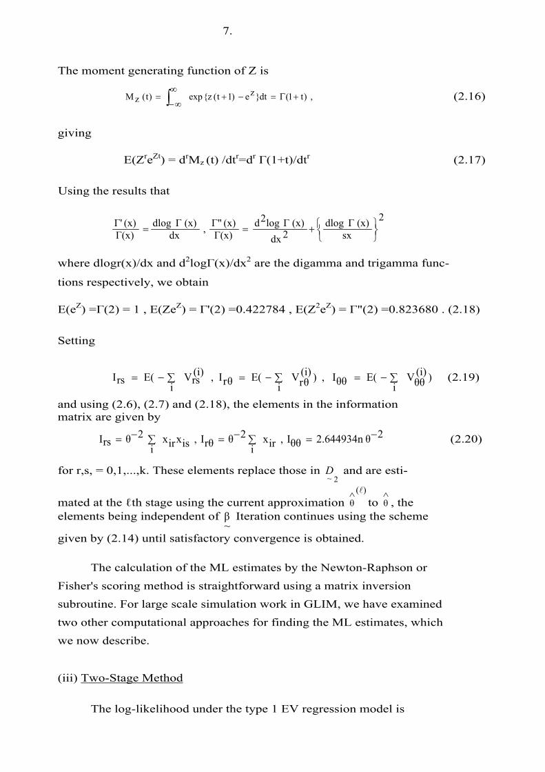
7. The moment generating function of Z is

(2.16),)t1(dt}ze)1t(z{exp)t(zM +Γ=−+∞

∞−= ∫

giving

E(ZreZt) = drMz (t) /dtr=dr Γ(1+t)/dtr (2.17)

Using the results that

2

sx(x) Γ dlog

2dx(x) Γ log2d

Γ(x)(x)Γ",dx

(x) Γ dlogΓ(x)

(x)Γ'⎭⎬⎫

⎩⎨⎧+==

where dlogr(x)/dx and d2logΓ(x)/dx2 are the digamma and trigamma func-

tions respectively, we obtain

E(eZ) =Γ(2) = 1 , E(ZeZ) = Γ'(2) =0.422784 , E(Z2eZ) = Γ"(2) =0.823680 . (2.18)

Setting

(2.19) )(i)θθV

iE(θθI,)(i)

rθVi

E(rθI,(i)rsV

iE(rsI ∑−=∑−=∑−=

and using (2.6), (2.7) and (2.18), the elements in the information matrix are given by

22.644934n θθθI,irxi

2θrθI,isxirxi

2θrsI −=∑−=∑−= (2.20)

for r,s, = 0,1,...,k. These elements replace those in and are esti- 2~

D

mated at the ℓth stage using the current approximation to )(l∧

θ∧θ , the

elements being independent of Iteration continues using the scheme

given by (2.14) until satisfactory convergence is obtained. ~β

The calculation of the ML estimates by the Newton-Raphson or

Fisher's scoring method is straightforward using a matrix inversion

subroutine. For large scale simulation work in GLIM, we have examined

two other computational approaches for finding the ML estimates, which

we now describe.

(iii) Two-Stage Method

The log-likelihood under the type 1 EV regression model is

8

. γ θ ~ β '

i ~ x

i y

exp i

) ~ β '

i ~ x i (y

i 1 θ n γ θ n log θ)

~ β L(

⎟ ⎟ ⎟ ⎟ ⎟

⎠

⎞

⎜ ⎜ ⎜ ⎜ ⎜

⎝

⎛

− −

∑ − − ∑ − + − − = (2.21)

Consider a fixed value of 0, say ℓ. Putting β*0 = γ + θ ,β1

0−

0 , β*r = θ β10−

r , r = 1,...,k

n,...,1i,)*~β'

i~xexp(iu,)0

/θi

exp(yiy ==∗=∗

we have

)i*/ui*(y

ii*ulogi0θlogni*logy

i)0θ,*~

βL( ∑−∑−−∑= (2.22)

Maximising with respect to )0,~

(L θβ~β is therefore equivalent to

maximising )i*/ui*yi*ulog

i)0θ,*~

βL( +∑−= (2.23)

with respect to )0θ,*~β(1L.

*~β is the log-likelihood treating the

{y*i .} as observations on independent exponentially distributed observ-

ations with means {µ*i }, where logµ*i *~β'

i~x The value )( 0*~β

*~β θ

∧=

∧

which maximises )0θ,*~β(1L may therefore be obtained using GLIM by

specifying an exponential error distribution and a logarithmic link function.

Treating~β as known, the value )

~(βθθ

∧=

∧ of 8 which maximises )θ,

~βL(

is from (2.9) a solution of the equation )~β,θ(g

∧ = 0 where

.θn1γθ~β'

i~x

iy

xp)~β'

i~xi(yi

)~β,θg(

∧−

⎪⎪⎭

⎪⎪⎬

⎫

⎪⎪⎩

⎪⎪⎨

⎧

−⎟⎟⎟⎟

⎠

⎞

⎜⎜⎜⎜

⎝

⎛

−−

−∑=∧ (2.24)

Using a Newton-Raphson approach to find an iterative solution for 0, if θ ℓ. denotes the ℓ th approximation to θ , we have

,)~β,θg(/)

~β,θg(θ1θ llll

∧∧−

∧=+

∧ ℓ = 1,2,.. . (2.25)

Since in practice both~β and are unknown, the following two—stage

iteration method may be used. If 1,~

∧θ

∧β denote preliminary approx-

imations to respectively, the new approximation ∧θ

∧β and~

2 is given by

.)1~β,1θ(g'/)

1~β,1θg(1θ

∧∧∧=

∧ ∧ The transformed observations ∧

θ= )2/iyexp(i*y

are then used in a GLIM fit to obtain∧β

2*~and hence

∧β2~. The same steps

are used repeatedly until satisfactory convergence is obtained.

9

(iv) The Roger/Peacock Method An alternative method specially designed for work in GLIM was proposed by Roger and Peacock (1982). Their method copes with censored observations and has the advantage over the preceding method of providing the estimated asymptotic covariance matrix of the ML estimates directly from the output of a GLIM fit. To apply their method, we put

,γθ~β'

i~xiyexp*

iμ,1/ θα⎟⎟⎟

⎠

⎞

⎜⎜⎜

⎝

⎛−

−== i = 1 ,...,n . (2.26)

We have

i = 1 ,.. , ,n (2.27) ,*~β*

i~xiy α*iμlog +=

where ’ = { - (α β*

~β 0 + γ) , - α β 1 ,...,-α β k, } and the log-likelihood may

be written as

(2.28) .αlogn)*iμ

*iμ(log

n

1iα),*

~βL( +−∑

==

Let denote the ML estimates of α and. To use GLIM, we may *^

~

^, βα *

~β

proceed as follows. Suppose that we have n independent Poisson random variables Z1 ,...,Zn with means µ1

* ,,..,µ*n satisfying (2.27), and an

independent binomial random variable Zn+1 based on n trials and 'success1

probability α: The log-likelihood for realised values z1 , ,,.,zn and zn+1 is

.α)(1log)1nz(nαlog1nz)*iμ

*ilogμi(z

n

1iconstant

1nznα)(11nzαn1nzlog

iz

zi*iμ

*iμe

logn

1iα),*

~β(1L

−+−+++−∑=

+=

⎭⎬⎫

⎩⎨⎧

+−−+⎟⎠⎞

⎜⎝⎛

++

⎟⎟⎟⎟

⎠

⎞

⎜⎜⎜⎜

⎝

⎛ −

∑=

= (2.29)

For the specific realisation zi = 1, i = 1 ,. . . ,n and zn+1 = n, we have

α),*~β(1L α),*

~β(L= + constant. Hence maximisation of ),*

~(L αβ is equiv-

alent to maximisation of the log-likelihood based on the random variables Z1.,...,Zn and Zn+1 , , when the realised values are z.=1, i = 1 , . . . ,n for the Poisson variables and zn+1 = n for the binomial variable. Roger and Peacock give a GLIM program, containing five macros including four macros for fitting a user-defined model, which may be used to find the ML estimates.

10

Some idea of the variations in computer time required to determine the ML estimates can be obtained from table 1 which shows the computer processing units (CPU) for each of the four methods of estimation for 10, 20 and 50 sets of sample data generated by simulation for n = 25. The results indicate that the Fisher-scoring method requires less time than the Newton-Raphson method and gives considerable savings over the two-stage method. Comparisons with the Roger/Peacock method are more difficult to make, as the stopping rule for convergence is not controlled by the user but is implemented in the GLIM system. Further, a run with 100 sets of data showed that in a few cases the Roger/Peacock method failed to produce a solution because negative values were produced for the total deviance.

Table

CPU usage for four methods for obtaining ML estimates

Run Size Roger/Peacock Fisher scoring Newton-Raphson Two Stage10 59 sec 74 sec 83 sec 115 sec 20 108 sec 150 sec 151 sec 216 sec 50 255 sec 334 sec 458 sec 626 sec

3. Moment Properties Of The Maximum Likelihood Estimators

The exact moments of the ML estimators are unknown, but approximations to their biases, variances and covariances correct to 0(n-1 ) can be obtained by standard methods.

Without loss of generality, we shall assume that the values of the x's

are centred such that for r = 1,...,k. In this case, use of 0irxn

1i=

=∑

(2.20) shows that theinformation matrix may be written as

(3.1) ⎟⎟

⎠

⎞

⎜⎜

⎝

⎛−=2~I~O

~O1~I2θ~I

where1~I refers to θ and β 0 irefers

2~I to β 1..., β k and

. (3.2) =⎟⎠⎞

⎜⎝⎛

−=

2~Inn

n2.64493n1~I

⎥⎥⎥⎥⎥⎥

⎦

⎤

⎢⎢⎢⎢⎢⎢

⎣

⎡

∑∑∑

∑∑∑

∑∑∑

2ikx

iikxi2xiikxi1x

i

ikxi2xi

..2i2x

ii2xi1xi

ikxi1xi

..i2xi1xi

2i1x

i

11 Since

⎟⎠⎞

⎜⎝⎛ −

−−=− 6079.0

6079..06079..06079.0

1n1~I

we have the standard approximations

var .n20.6079 θ)

^θ,0

^β(cov,n

20.6079 θ)^θ(var,n

21.6079 θ)0^β( −≈≈≈ (3.3)

The approximate covariance matrix for = is)kβ,....,1β('

1~β =

. (3.4) 1))isxirxi

((2)1

^

~(Cov −θ≈β ∑

To obtain the approximate biases, we first need the third order derivatives of the logarithm of the density given by (1.6). Setting

3)iy(iYflog3

)i(W,2

r

)iy(iYflog3)i(

rW,sr

)iy(iYflog3)i(

rsW,tsr

)iy(iYflog3)i(

rstWθ∂

∂=θθθ

θ∂β∂

∂=θθθ∂β∂β∂

∂=θβ∂β∂β∂

∂=

(3.5)

and using the second order derivatives given in (2.6) and (2.7) we obtain

(3.6) 2)γi(zizeisxirx3θ(i)

rs θW,izeitxisxirx3θ (i)

rstW ++−= −=

= θ)i(rW θθ

-3 xir [ {zize i. + γ ) 2 + 4 (zi + γ) + 2 } - 2] (3.7)

)i(Wθθθ = θ-3 [ iz

e X{(zi +γ)3 +6 (zi + γ)2 +6(zi + γ) } -6(zi +γ) -2] . (3.8) We set

)(i)θθθW

iE(θθθK,)(i)

rθθWi

E(rθθ)K(i),rsθW

iE(rsθK,)(i)

rstWi

E(rstK ∑=∑=∑∑= (3.9)

Using (2.17) we obtain

E{(Z + γ)exp(Z:)} - Γ'(2) + γ = 1 (3.10) E{(Z + γ)2exp(Z)} = Γ"(2) + 2γΓ'(2) + γ2 = 1.64494 (3.11) E{(Z+γ)3exp(Z)} - Γ"' (2) + 3γΓ"(2) + 3γ2Γ'(2) + γ3 = 2.53070 (3.12)

and hence

12

(3.14)n316.4.003 θθθθK,irxi

35.64494 θrθθK

(3.13)isxirxi

33θrsθK,itxisxirxi

3θrstK

−=∑−=

∑=∑−= −

Finally, we require the values of the quantities

{ }

{ }[ ]

{ }[ ]{ }[ ]

{ } { }[ ]

{ } { }[ ] (3.20)11)Z(eγ)2(ZZe2γ)(Z11)Z(eγ)(ZE3nθ

)(i)θθV(i)

θUi

(Eθθθ,J

(3.19)Z1)eZ(eγ)(Z1Ze11)Z(eγ)(ZEisxi

3θ

(i)sθV(i)

θUi

(Esθθ,J

(3.18)11)Z(eγ)(ZZeEitxisxi

3θ(i)stV(i)

rUi

(Estθ,J

(3.17)11)Zγ)e2(ZZe2γ)(Z1)Z(eEirxi

3θ

(i)θθV(i)

rUi

(Eθθr,J

(3.16)γ)(ZZe1Z(e1)Z(eEisxirxi

3θ(i)sθV(i)

rUi

(Esθr,J

(3.15)1)Z(eZeEitxisxirxi

3θ(i)stV(i)

rUi

(Estr,J

−−+++−−+−−=

∑=

−++−−−+∑−−=

∑=

−−+∑−−=∑=

−−+++−∑−−=

∑=

++−−∑−−=∑=

−∑−−=∑=

Using (2.17) we have E{Zr exp(2z) } = dr (x)/dxr evaluated at x = 3 which gives

E(e2Z) = r(3) = 2 , E(Ze2Z) - T'(3) = 1.84557

E(Z2 e 2Z) = Γ"(3) = 2.49293 , E(Z3e2Z) = Γ"'(3) = 3.44997 .

Use of these results in (3.15) to(3.20) gives after simplification

(3.21)n.311.11040 θθθθ,J,isxi

33.64493 θstr,J

(3.22)itxisxi

3θstθ,J,irxi

35.64493 θθθr,J

(3.21)isxirxi

33θsθr,J,itxisxirxi

3θstr,J

−−=∑−−=

∑−−=∑−−=

∑− −−=∑−=

13

denote the biases of and θ, θ)^θE(θbandrβ)r

^βE(rbIf −=−= r

^β

respectively, r = 0,1,..., k, then from Cox and Snell (1968) the bias approximations correct to 0(n ) are

(3.25))sut,J2stu(KutIθsI

uts21

θb

(3.24))sut,J2stu(KutIrsI

uts21

rb

+∑∑∑−=

+∑∑∑−=

where the summations are over s,t ,u = 0,1,...,k, θ and Irs, I θS etc. denote elements in the inverse of the information matrix.

Simple expressions for the biases can be obtained straightforwardly for the case when the x's satisfy the conditions

0 for all r ≠ s = 0,1,...,k . (3.26)isXirXn

1i∑=

The elements in the inverse of the information matrix are then

I00 = 1.6079n-1 θ2 , Iθθ = 0.6079n-1θ2 , Irr = θ2/Σixir.

for r = 1 ,... ,k (3.27)

Iθθ = -0.6079n-1θ, Ir0 = Irθ = Irs = 0 for r ≠ s - 1 , . . . ,k (3.28)

with the regression coefficient estimators rβ , r = 0,1,...,k being pair-wise asymptotically uncorrelated. We may write

rArrI21,)θAθ0I0Aθ0(I2

1θb,)θA0θI0A00(I2

1cb =+=+= (3.29)

for r = 1,...,k, where

∑ ∑ +∑=+∑=t t

)θut,2Jθtu(KtuIuθA,)rut,2Jrtu(KtuI

urA (3.30)

A straightforward calculation gives

(3.31)1θ3.9304)(3kθA,)2itX

i/2

itXirXi

k

1t1θrA,11.3921)θ(k0A −+−=⎟

⎠⎞

⎜⎝⎛

∑∑∑=

−−=−+−=

from which we obtain

b0 = θn-1(0.1080k + 0.0754) , (3.32)

14

K...,1r,2itX

i/2

itXirXi

k

1t2irX

i

21

rb =⎟⎟⎟

⎠

⎞

⎜⎜⎜

⎝

⎛

=

θ−= ∑∑∑

∑ (3.33)

bθ = -θn-1(0.6079k + 0.7715) . (3.34)

In the case of a single explantory variable x with values centred such that these bias expressions give ,0iX

i=∑

θ1.3794n1^θ

b,2)2iX

i(/3

iXi

θ21

1b,θ10.1834n0b −−=∑∑−=−= . (3.35)

An important property which can easily be deduced from the likelihood equations is that the random variables

k...,1,0,r,say(1)r

^βr/θ)rβr

^β(,say(1)θ/θ

^θ ==−= (3.36)

are distributed independently of

~β and 0. Thus from (2.9) the likelihood

equations depend on which may be written as iZ

γ(1)^θ/)(1)

~β'

i~xi(ui^Z −−=

where

(3.37).n,...1,i,)~β'

i~xi(y1θiu =−−=

The {ui} are independently and identically distributed with p.d.f. fU (u) = exp(u - γ - eu-γ ) , -∞ < u < ∞ which is the standardised type 1 EV distribution for smallest values and which does not depend on or θ It follows that the joint dis-

~β

tribution of the random variables and(1)θ(1)

~β is the same as that

of the ML estimators of 9 and when the 'observations' {ui} have the

p.d.f. given by (3.38). Consequently, (1)

~β and are distributed (1)θ

independently of and θ. ~β

It is straightforward to show that the above distribution property

for and(1)θ(1)

~β holds generally for the class of regression models with

(y) = θ-1 f{y-µi)/0}, where This generalises the result ~β'

i~xiu −iYf

given by Antle and Bain (1969) for the case when no explanatory variables are present.

15

In order to examine the adequacy of the bias and variance approx-

imations and to assess other moment properties of the ML estimators, a

Monte-Carlo simulation investigation was made for the case of simple

linear regression with grouped data, the model being

Yij = βo + βix

i + εij , i = 1, . . . g j = 1,...,mi (3.39)

where }ij{Ytheand2θ2πθ1)ij(εvar,0)ijE(ε == are independently

distributed with p.d.f. given by

.y,γθiX1β0βy

expγθiX1β0βy

expθ1(y)ijYf ∞<<∞−

⎭⎬⎫

⎩⎨⎧

⎟⎟⎠

⎞⎜⎜⎝

⎛−

−−−−

−−= (3.40)

Equally spaced values of x were taken with21iiX −= (g + 1) , i - 1,...,g.

Equal sample sizes mi = m = 1,2,5(5)20 for i = 1 ,. .. ,g were used with g = 5,10. Without loss of generality, the values

~~0β = and θ = 1 were

used, the y-variate observations for the simulation being generated by

sampling the distribution with density given by (3.38). The ML estimates

were found correct to at least four decimal places using Fisher's scoring

method. In each case, two independent runs each of size 2000 were made

and the moment results then averaged over the two runs.

Values of the biases and variances of the ML estimates as obtained

by simulation are shown in tables 2, 3, 4 for β0, β1 and θ respectively.

The approximations to the biases and variances are also shown.

The results show that the approximate biases given by (3.35) agree quite well with the biases obtained by simulation even when m is very

small. Further the biases in are appreciably larger than the biases ^

θof the ML estimates of the regression coefficients. The large sample approximation for the variance of works well for all m but the ^

~0β

approximating variance of underestimates the true variance when ^

~0β

m = 1,2. In the case of ,the approximating variance given by (3.3) ^θ

generally agrees well with the values obtained by-simulation, but there is some overestimation of the variance when m = 1 and g = 5.

16

Table 2

Biases x 102 θ-1 and variances x 10 2 θ-2 of the ML estimates of β

Bias Variance Simul Approx (3 .35) Simul Approx (3.3)

m

g=5

g = 10

1 3.07 3.67 2 1 .34 1 .83 5 0.73 0.73

10 -0.08 0.37 15 0.35 0.25

20 0.15 0.18

1 2.53 1 .83

2 0.77 0.92 5 0.40 0.37

10 0.02 0. 18 15 0, 19 0.12 20 -0.20 0.09

32.423 32.158 15.631 16.079 6.575 6.432 3.158 3.216 2.118 2.144

1.580 1 .608

15.807 16.079

7.853 8.040 3. 152 3.216 1 .591 1 .608 1 .075 1 .072 0.825 0.804

Table 3

Biases × 10 θ and variances x 10 θ of the ML estimates of β2 -1 2 -21

g=5

g-10

Bias Simul Approx (3 .35)m 1 -0.48 0.002 0.40 0.005 -0.29 0.00

10 -0.14 0.0015 -0.06 0.00

20 0.13 0.00

1 -0.12 0.00

2 0.00 0.005 0.12 0.00

10 0.08 0.0015 0.12 0.0020 0.07 0.00

Variance S imul Approx (3.4)

14.241 10.0005.705 5 .000

2. 130 2.0001 .017 1 .0000.681 0.667

0.507 0.500

1 .491 1 .212

0.670 0.6060,260 0.2420.124 0.1210.082 0.0810.061 0.061

17

Table 4

Biases x 102 θ-1 and variances x 102 θ-2 of the ML estimates of θ

Bias Variance

Simul Approx (3.35) Simul Approx (3.3)

m

g=5

g=10

1 -29.87 -27.592 -14.51 -13.79

5 -5.78 -5.52

10 -2.61 -2.76

15 -1 .89 -1.84

20 -1.37 -1.38

1 -14.94 -13.79

2 -7.05 -6.90

5 -2.93 -2.76

10 -1.31 -1.38

15 -0.87 -0.9220 -0.67 -0.69

10.357 12.158

5.743 6.079

2.417 2.432

1.241 1.216

0.826 0.811

0,598 0.608

5.944 6.079

2.931 3.040

1.238 1.216

0.608 0.608

0.411 0.4050.314 0.304

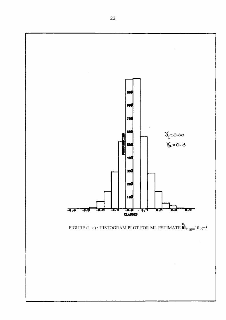
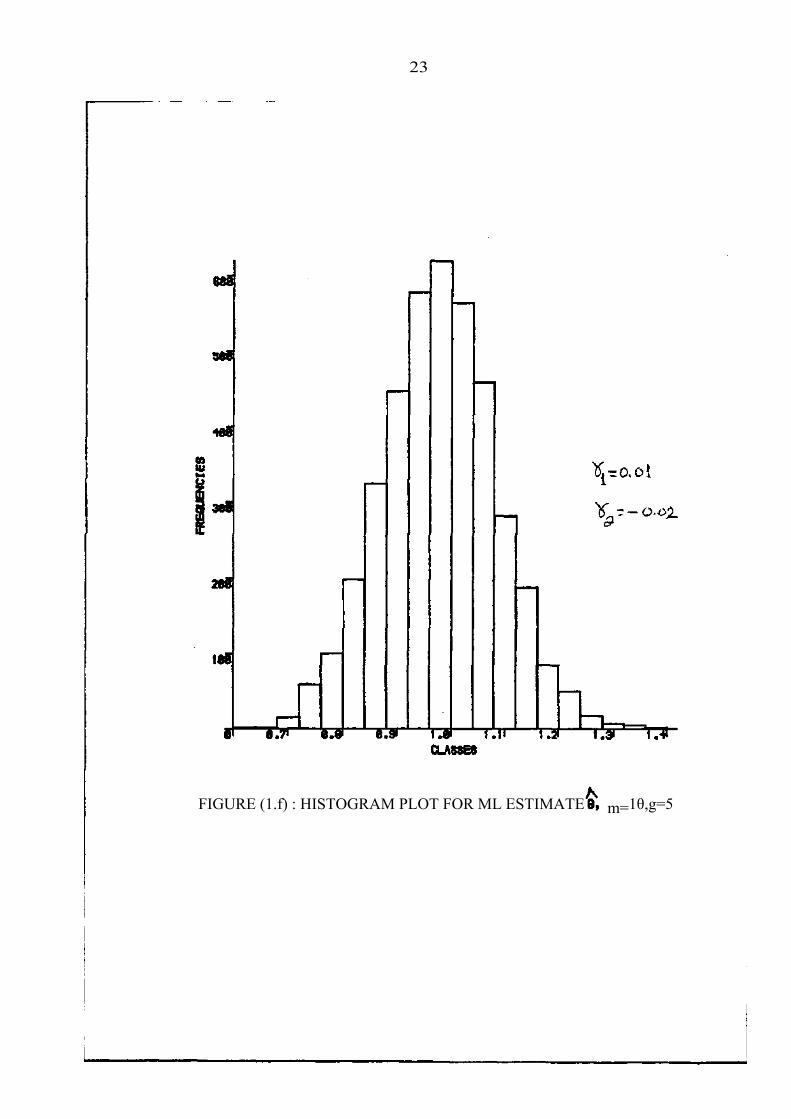
The shapes of the distributions of the ML estimates can be seen from

the histogram plots which are shown in figures la,..., "If. Values of the

skewness coefficient γ1 (β ) 0ˆ

0β θt γ1( ), γ1( ) and the kurtosis coefficients

γ2( ), γ0β 1β θ2( ) γ2( ) as obtained by simulation are also given correct

to 2 decimal places . These must be treated with caution as their sampling

errors are quite large even for the run-size of 4000 used in the investi-

gation. The plots and the coefficients indicate that the distributions

are reasonably close to the normal even for these moderately small values

of m.

18

FIGURE (1.α ) : HISTOGRAM PLOT FOR ML ESTIMATE , m=5,g=5 ^βθ

19

FIGURE (1.b) : HISTOGRAM PLOT FOR ML ESTIMATE m=5,g=5

20

FIGURE (1.c) : HISTOGRAM PLOT FOR ML ESTIMATE m=5,g=5

21

FIGURE (1.d) : HISTOGRAM PLOT FOR ML ESTIMATE m=1θ,g=5

22

FIGURE (1.,e) : HISTOGRAM PLOT FOR ML ESTIMATE m=1θ,g=5

23

FIGURE (1.f) : HISTOGRAM PLOT FOR ML ESTIMATE m=1θ,g=5

24

We have noted that the results in table 4 show that the bias and

variance approximations for work well even for moderately small values ^θ

of n and that the bias is considerably larger than the standard deviation.

Further the biases of the estimator^θ are much larger than those of the

estimatorsβ andβ , This suggests that it may be worthwhile considering ^ ^0 1

estimators of θ with reduced bias and possibly an improved mean square error performance. Two such estimators are now developed.

Setting c = 1.3794 and a = 0.6079 we have to order n

1n2aθ)^θvar(,1n θ c^

θb −=−−=

which gives the approximation

. (3.41))2n2C1(an2θ)^θmse( −+−≈

An estimator having bias of order n is given by

(3.42)^θ)1cn(1

^*θ −+=

with Ignoring terms of order n.2θ/n2c^*θb −≈ -3 and smaller terms,

we have the approximation

(3.43))22acn1(an2θ)^*θmse( −+−≈

so the proportionate reduction in the mse" is

.1.9020.6.8n0.226

2can2ac2C

)^θmse(

)^*θmse()

^θmse(

+=++≈− (3.44)

An alternative estimator of the form can be ^θ)1kn(1

*^*θ −+≈

considered, where k is selected to minimise the approximating mse of the estimator. The bias and variance of to order n**θ -1 are

(3.45)1n2aθ2k*)*^θ(var,}2kcn1c)n(kθ{**

^θb −=−−−−=

giving the approximation

[ ] .}2c)(k{2ak2n1an2θ)*^*θmse( −+−+−≈ (3.46)

Setting ∂ mse gives k = c - a, so the estimator is 0k/*)*^θ( =∂

(3.47) ^θ)10.7715n(1

*^*θ −+=

25 with an associated approximate mse

.)2n)2a{2ac1an(2θ*)*^θmse( −−+−≈ (3.48)

The proportionate reduction in the mse compared with the ML estimator

is ^θ

.1.9030.6.8n0.595

2can

2a)(C

)^θmse(

)^*θmse()

^θmse(

+=+

−≈− (3.49)

Values of the biases and mse's of the estimates , and ^θ *

^θ **

^θ

as estimated by simulation are shown in table 5.

The results show that the bias reduction estimator has a *^θ

much better bias performance than the ML estimator . Its mean square ^θ

error performance is also much better when m= 1, but for m> 1 the diff-

erences in mean square error are small. The estimator generally **^θ

has a slightly improved mean square error performance compared with ^*θ

but it has a poorer bias performance.

Table 5

Biases × 102 θ-1 and mse's × 102 θ-2 of the estimators ^θ *

^θ **

^θ

Bias mse

**^θ*

^θ

^θ**

^θ*

^θ

^θm

g=5

g=10

1 -29.87 -10.52 -19.052 -14.51 -2.71 -7.915 -5.18 -0.58 -2.87

10 -2.61 0.08 -1.1115 -1 .89 -0.08 -0.8820 -1 .37 -0.01 -0.61

1 -14.94 -3.21 .-8.38

2 -7.05 -0.64 -3.465 -2.93 -0.25 -1.43

10 -1.31 0.05 -0.55

15 -0.87 0.05 -0.3620 -0.67 0.02 -0.29

19.280 17.967 17.4297.847 7.510 7.2882.755 2.694 2.6511.310 1.310 1.2920.862 0.857 0.851

0.617 0.615 0.61 1

8.179 7,800 7.598

3.428 3.353 3.2811.326 1.308 1 .2960.625 0.625 0.6200.419 0.419 0.4170.319 0.318 0.318

26 4. Moment Properties Of The Ordinary Least Squares Estimators

The OLS estimator of ~Y'~X1)~X'~X(

~

~βis

~β −= showing that the individual

parameter estimates r = 0,1,...,k, are linear functions of the {Y,βr

~i},

whose moments are known exactly. It follows that the exact moments of

the }r~β( can be found. The estimators are unbiased and we have

.1)~X'~X(2θ2π6

1)~

~β(cov −= (4.1)

Assuming that for r = 1 k we have 0irXn

1i=∑

=

.))isxirxi

((2~

Iwhere,0

2~I

n0~X'~X ∑=

⎥⎥

⎦

⎤

⎢⎢

⎣

⎡=

Hence we have

/n21.6449 θ/n2θ2π61)0β

~(var == (4.2)

and the covariance matrix of ~

isβk)...1,~β

~0β(

~

1~β =

.1))isxirxi

((21.6449 θ12~I

2θ2π61)

1~β~cov( −∑=−= (4.3)

The exact skewness and kurtosis coefficients of can be found using ,~

rβ

the following results due to Scheffé (1959). Let be a ii

n

iYC∑

==

1ξ

linear combination of n independent random variables {Yi} where Y. has variance σ1

2, skewness coefficient γi,i . and kurtosis coefficient γ2, i . .. Then the skewness and kurtosis coefficients for ξ are given by

where (4.4) .2

iσ2iC

i/2

iσ2iCiα

i2,γ2iα

n

1iξ2,γi1,γ3/2iα

n

1iξ1,γ

∑=

∑=

=∑=

=

We let cir denote the i th element in the rth row of so'~X1)~X'~X( −

~,2.4000i2,γ,1.2986i1,γ,2θ2π6

12iσwith,iYirC

n

1ir β ===∑=

=

i - 1,...,n. Hence use of (4.4)gives

(4.6)2irC

i/4

irCn

1i2.4)rβ

~(2γ

(4.5)3/2)2irC

i(/3

irCn

1i1.2986)rβ

~(1γ

∑∑=

=

∑∑=

=

for r = 0,1,...,k.

27

For the OLS estimator of 9, approximate bias and variance results ~θ

can be obtained using the exact results available for the mean and variance

of The LS estimator is unbiased for 2~

θ2~

σ σ 2 and from Atiqullah (1962), its exact variance is

⎪⎭

⎪⎬⎫

⎪⎩

⎪⎨⎧

−∑−−+−−= 2)iih(1i1kn

2γ2111kn

42σ)2~σ(var (4.7)

where γ2 is the coefficient of kurtosis of the distribution of the response variable Y and hii.- is the ith diagonal element in the 'hat' matrix

'~X1)

~X'

~X(

~X

~H −=

For the type 1 EV distribution we have γ2 = 2.4 and

hence the unbiased estimator of θ2 given by

}21)πk(n{/2)~

~β'

i~Xi(Yi

62~θ −−−∑= (4.8)

has exact variance

.2)iih(1n

1i1kn1.211kn

42θ)2~θ(var

⎭⎬⎫

⎩⎨⎧ −∑

=−−+−−= (4.9)

Writing

...)2(8θ/2)2θ2~θ(θ) (2/)2θ

2~θ(θ2

1}2/θ)2θ

2~θ(θ{1

~θ −−−+=−+=

and using the result that tr( ~H ) = k+ 1 we obtain to order n-1 ,

)10.55nθ(1)~θE( −−= (4.10)

var = 1.1n)~

(θ -1 θ2 . (4.11)

Table 6 gives values of the exact variances skewness and )2x( −θ

kurtosis coefficients for the OLS estimators~0β and

~β for the simple 1

linear regression model considered in the presvious section. Table 7

shows values of the approximate biases and variances of the OLS estimator

θ~ given by (4.10) and (4.11) for the same model. The biases and vari-

ances of θ~ as obtained by simulation are also shown, the simulation again

using a run-size of 4000.

28

Table 6

Exact variance (x 102 θ -2 ), skewness and kurtosis coefficients of

the OLS estimators 1~β0

~β

0~β

~1β

g=5

g=10

m var. skew. kurt.

1 32.899 0.58 0.102 16.449 0.41 0.025 6.580 0.26 0.00

10 3.290 0.18 0.0015 2. 193 0. 15 0.0020 1 .645 0. 13 0.00

1 16.449 0.41 0.02

2 8.225 0.29 0.015 3.290 0.18 0.00

10 1.645 0.13 0.00

15 1.097 0.11 0.0020 0.823 0.09 0.00

var. skew. kurt.

16.449 0.00 0.08

8.225 0.00 0.02

3.290 0.00 0.001.645 0.00 0.001.097 0.00 0.000.823 0.00 0.00

1 .994 0.00 0.01

0.997 0.00 0.00

0.399 0.00 0.00

0. 199 0.00 0.000. 133 0.00 0.000. 100 0.00 0.00

Table 7Biases and variances ( x 102 θ -2 )

Bias Variance

g=5

g=10

App. (4.11) Simul22.000 18.92111.000 9.413

4.400 3.9292.200 2.060

1.467 1.4611.110 1.074

11.000 9.623

5.500 4.9162.200 2.126

1.100 1.0580.738 0.7590.550 0.540

m App. (4.10) Simul1 -11.00 -10.40

2 -5.50 -5.215 -2.20 -2.43

10 -1.10 -1 .0315 -0.73 -0.88

20 -0.55 -0.66

1 -5.50 -5.60

2 -2.65 -2.685 -1.10 -1.16

10 -0.55 -0.6315 -0.37 -0.3520 -0.27 -0.32

29

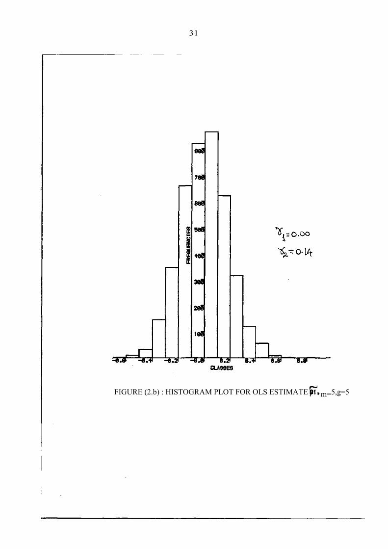
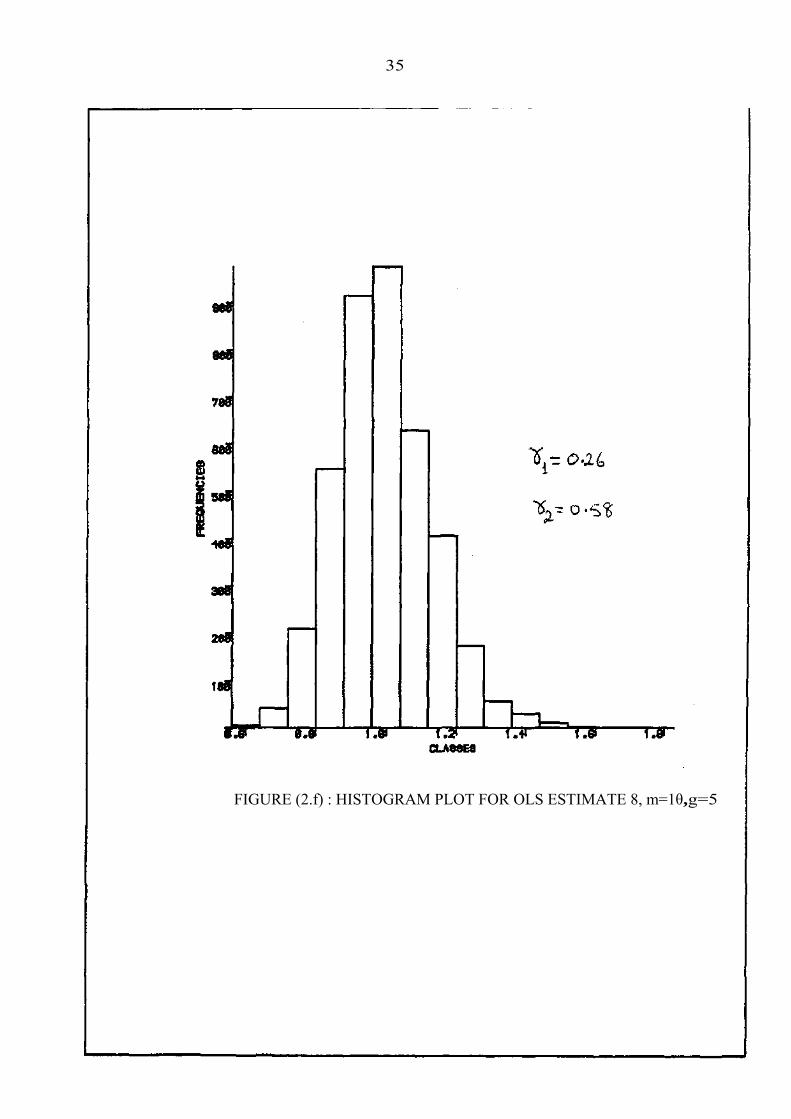
Histogram plots of the distributions of 0β~ , 1β

~ , and θ~ as generated

by simulation are shown in figures 2a,...,2f for g = 5 and m = 5,10. The values of the skewness and kurtosis coefficients for θ~ are also shown. The plots show that the distribution of the estimators are close to the normal.

30

FIGURE (2.α) : HISTOGRAM PLOT FOR OLS ESTWATE m=5, g=5

31

FIGURE (2.b) : HISTOGRAM PLOT FOR OLS ESTIMATE m=5,g=5

32

FIGURE (2.c) : HISTOGRAM PLOT FOR OLS ESTIMATE m=5,g=5

33

FIGURE (2.d) : HISTOGRAM PLOT FOR OLS ESTIMATE m=10,g=5

34

FIGURE (2.e) : HISTOGRAM PLOT FOR OLS ESTIMATE m=1θ,g=5

35

FIGURE (2.f) : HISTOGRAM PLOT FOR OLS ESTIMATE 8, m=1θ,g=5

36

5. Best Linear Unbiased Estimators Based On Order Statistics For Grouped Data

In this section, we shall assume that we have g distinct sets of values xil, ...,x ik , i = 1,...,g for the explanatory variables and suppose that mi observations on Y are made at the point (xi1 , . . . ,xik ) .

We let n = ∑ m

=

g

1ii. denote the total number of observations. With grouped

data, it is possible to find the best linear unbiased estimates (BLUE's) of the {βr } and θ based on the order statistics within the groups. These estimators are asymptotically as efficient as the ML estimators and have appreciably smaller variances than the OLS estimators.

We first need some results for the case when a single random sample of m observations is drawn from a population with the type 1 EV c.d.f.

{ },ξ)/θ(yeexp1F(y) −−−= —∞ < y < ∞ . (5.1)

It is convenient to allow for censoring. Thus if Y(1) < Y(2) , < ... < Y (m)

denote the order statistics in the sample, we shall assume that only The first r order statistics observed. We let

(5.2)(i)Yibr

1i*^θ,(i)Yia

r

1i

^*ξ ∑

==∑

==

denote the BLUE's for ξ and θ respectively, that is we require ,)*^

(E ξ=ξ

)*

^θE( = 0 and var ≤ var, var ≤. var , where ,denote )

*

^ξ( )'

^(ξ )

*^θ( )*

^(θ

any other linear unbiased estimators of ξ and θ, respectively.

If we put X(i) = (Y(i)-ξ)/θ , i = 1, ...r, then X(1),X(2) , .. .,X(r) are distributed as the first r order statistics in a random sample of m observations from the standardised type 1 EV distribution with c.d.f. F(x) = 1 - exp(-expx), - ∞< x < ∞. Putting

E(X(i)) = ei,m, cov(X(i),X(j)) = ci j ,m (5.3)

we have

E(Y(i)) =ξ + θ ei , cov(Y(i),Y(j) ) - θ2i j, m3. (5.4)

In matrix form, we have the linear model representation

(5.5) ~C2θ)

(.)~Y(cov,~n~A)(.)~YE( ==

37

θ), ξ ('~n,)(r)Y....,,(2)Y,(1)(Y'(.)~Ywhere ==

(5.6)

mrr,Cmr1,C....

m2r,C...m21,Cm1r,C...m11,C

~C,

mr,e1......

m2,e1m1,e1

~A

⎥⎥⎥⎥⎥⎥

⎦

⎤

⎢⎢⎢⎢⎢⎢

⎣

⎡

=

⎥⎥⎥⎥⎥⎥⎥

⎦

⎤

⎢⎢⎢⎢⎢⎢⎢

⎣

⎡

=

From generalised least squares theory, the BLUE for ~n is

.21)~A1

~C'

~A()

^

~n(covwith

(.)~Y1

~C'

~A1)

~A1

~C'

~A(

^

~n θ−−=−−−= The linear co-

efficients ai = ai (r,m) and bi = bi(r,m) giving the BLUES are obtained as the elements in the first and second rows of the matrix

1~C'

~A1)

~A1

~C'

~A( −−−

which -is of order 2 × r. Further, writing

⎥⎥

⎦

⎤

⎢⎢

⎣

⎡==−−

(3)mr,V(2)

mr,V

(2)mr,V(1)

mr,V~V

1)~A1

~C'~A( (5.7)

we have

va (ξ) = θ2V var (θ ) = θ,(1)r,m ˆ 2 V cov( ) , = θ,(3)

mr, θ,ξ 2 V . (5.8) (2)mr,

White (1964) gives tables of the linear coefficients {ai.} and

{bi} and the elements V , V , V (1)mr,

(2)mr,

(3)mr, required for computation of

the covariance matrix for 2 ≤ n ≤. 20 and r = 2(1 )n. The mean of the distribution given by (5.1) is µ = ξ - γθ so the BLUE for u is

(5.9)(i))Yiγbi(ar

1i*

^μ −∑

==

with

(5.10) saymVr,2θ)(3)r,mV2γ(2)

r,mV γ2(1)r,m(V2θ)

*μvar( =+−=

Suppose now that we have g populations, the c.d.f. for the ith population being

Fi(y) = 1 - exp[ - exp{(y- ξi)/θ}] , -∞ < y < ∞ (5.11)

38 i = 1,...,g. Let Yi(l), .. < Yi(2)., < ... < . denote the order statistics )ii(mY

in a random sample of mi. observations drawn from the ith population. If only the first ri order statistics Yi(1) , ., Yi(2) ..., , . are observed )ii(rY

for the ith group, the BLUE's are

(5.12),i(j)Yijbir

1j

^iθ,i(j)Yija

ir

1ji^ξ ∑

==∑

==

where aij = aj(ri ,mi) and bij = bj (ri,mi.) are the linear coefficients for best linear unbiased estimation. Since the { } are independent iθ

estimators of the assumed common θ with var( ) = θiθ2 V(3)

i,mir , the

minimum variance linear unbiased estimator of θ is

sayiθiwg

1i(3)im,ir

1/Vg

1i

(3)im,ir

/Viθg

1i*θ ∑

==

⎟⎠⎞

⎜⎝⎛

∑=

∑== (5.13)

where

1

)(3)i,mir

(1/Vg

1i(3)

i,mirViw

−

⎭⎬⎫

⎩⎨⎧

∑=

= , i = 1,…..,g . (5.14)

We have

(5.15).1)(3)i,mir

(1/Vi

2θ)*

^θ(var,θ)

*^θE( −

⎭⎬⎫

⎩⎨⎧

∑==

The best linear unbiased estimator of the mean µi. = ξi . - γθ for the ith group is

.*^θγi

^ξi*

^μ −= (5.16)

Using the result that cov we obtain ,2im,)2(

iVriW)^i,i

^(CoviW

^)*,i( θ=θξ=θξ

⎥⎦

⎤⎢⎣

⎡ −⎭⎬⎫

⎩⎨⎧

∑⎭⎬⎫

⎩⎨⎧ +−+= 1)(3)

im,ir/V(1

i2γ)(3)

im,irV/(2)

im,ir2γγ((1)

im,irV2θ)i*

^μ(var

= θ2w1i , say. (5.17)

Also

⎪⎭

⎪⎬⎫

⎪⎩

⎪⎨⎧

++−= )*

^θ(var2γ)i

^ξ,*

^θ(cov)i

^ξ,*

^θ(covγ)j*

^μ,i*

^μ(cov

39

)(3)

i,mirV/(1

i

2γ(3)j,mjr

V/j

(2)j,mjr

V(3)i,mir

V/(2)i,mir

Vγ2θ

∑

⎪⎭

⎪⎬⎫

⎪⎩

⎪⎨⎧

+⎟⎟⎟

⎠

⎞

⎜⎜⎜

⎝

⎛+−

=

= θ2 wij , say (5.18)

Since . is an unbiased estimator of µi*μ i. = we have the linear ~β'

i~x

model

i = 1,...,g (5.19) i*ε~β'

i~xi*^μ +=

where E( .) = 0, var( ) = θi*ε i*ε

2wii and cov( , ) = θi*ε j*ε2 wij. Setting

),g*ε,....,l*(ε'*~εand)g*μ,....,1*μ(

'*~

μ == the matrix form of the linear

model repres entation is

(5.20) *~ε~β

1~X*

^

~μ +=

with E( ) = *~ε ~0 and cov( ) = θ

*~εz

~W , where

(5.21).

gg....wg2wg1w..

2gw...22w21w1gw...12w11w

~W,

gkx...g1x1..

2kx21x11kx11x1

1~X

⎥⎥⎥⎥⎥⎥

⎦

⎤

⎢⎢⎢⎢⎢⎢

⎣

⎡

=

⎥⎥⎥⎥⎥⎥

⎦

⎤

⎢⎢⎢⎢⎢⎢

⎣

⎡

=

Based on the { }, the BLUE of is given by i*μ ~

β

,^

~μ1

~W'1~X

1)1~X

1~W

'1~X(*

^

~β −−−= (5.22)

with covariance matrix

cov (5.23).2θ1)1~

X1~W

'1~X()

*

^

~β( −−=

We now consider the important special case when the sample sizes are equal and the same degree of censoring occurs within each group, that is mi = m, ri. = r for i = 1,...,g. In this case we have

{ }

{ (5.25).say,w(2)mr,V γ2(3)

mr,V2γ1gijW

(5.24)say,V(2)mr,V γ2(3)

mr,V2 γ1g(1)mr,ViiW

=−−=

=−−+=

40

Letting w(i j) denote the (i,j)th element in -1

~W , we have

}w)1g(v){wv(w)ij(w,

}w)1g(v){wv(w)2g(v)ii(w

−+−−=

−+−−+

=

for i ≠ j = 1,2, . . . ,g.

putting

⎥⎥⎥⎥⎥⎥⎥⎥⎥⎥⎥

⎦

⎤

⎢⎢⎢⎢⎢⎢⎢⎢⎢⎢⎢

⎣

⎡

∑=

∑=

∑=

∑=

∑=

∑=

∑=

∑=

∑=

2ikx

g

1i...ikxi2xg

1i...ikxi1xg

1i

.

.ikxi2x

g

1i...2

i2xg

1i...i2xi1xg

1i

i1xi1xg

1i...i2xi1xg

1ii1xg

1i

~M

we may write

⎥⎥⎥⎥⎥⎥⎥

⎦

⎤

⎢⎢⎢⎢⎢⎢⎢

⎣

⎡

−−−−

−−−−

−−+−−+

=−

⎥⎥⎥

⎦

⎤

⎢⎢⎢

⎣

⎡

−−

−+=−−

gkx1w)(v...1kx1w)(v..

g1x1w)(v...11x1w)(v

11)w}(g{v...11)w}(g{v

1~W

'1~X,1

~Mw)(v~0~0g

1)w(gv1)

1~X1

~W'1~X(

(5.27) Since

⎥⎥⎥⎥⎥⎥

⎦

⎤

⎢⎢⎢⎢⎢⎢

⎣

⎡

=⎥⎥

⎦

⎤

⎢⎢

⎣

⎡

−

−=−

gkx...1kx..

g1x...11x1...1

'1~X,1

~M~0~0

1g1)1~X

'1~X( (5.28)

it follows that

(5.29) '1~

X1)1~

X'1~

X(1~W'

1~X1)

1~X1

~W'

1~X( −=−−−

showing that the OLS esimate of based on the { } provides the ~β i*μ

BLUE. It should be stressed that this result only applies when the

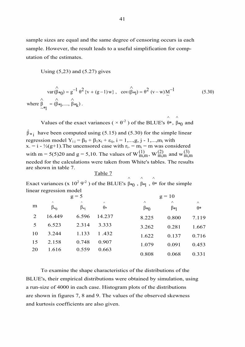
41

sample sizes are equal and the same degree of censoring occurs ia each

sample. However, the result leads to a useful simplification for comp-

utation of the estimates.

Using (5,23) and (5.27) gives

.)k*β....,,1*β(1*~βwhere

(5.30)1~Mw)(v2θ)1*β(cov,w}1)(g{v2θ1g)0*β(var

∧∧=

∧

−−=∧

−+−=∧

Values of the exact variances ( × θ-2 ) of the BLUE's , and *^θ 0*

^β

i*β have been computed using (5.15) and (5.30) for the simple linear regression model Yi j = β0 + β1xi + εij, i = 1,...,g, j - 1,...,mi with x. = i - ½(g+1).The uncensored case with ri. = mi = m was considered

with m = 5(5)20 and g = 5,10. The values of W(1) , W(2) and w(3) m,m mm, mm,needed for the calculations were taken from White's tables. The results are shown in table 7.

Table 7

Exact variances (x 102 9-2 ) of the BLUE's , , for the simple 0*^β 1*

^β *

^θ

linear regression model g = 5 g = 10

m 0*

^β

1*

^β *

^θ

2 16.449 6.596 14.237

5 6.523 2.314 3.333

10 3.244 1.133 1 .432

15 2.158 0.748 0.907 20 1.616 0.559 0.663

0*^β 1*

^β *

^θ

8.225 0.800 7.119

3.262 0.281 1.667

1.622 0.137 0.716

1.079 0.091 0.453

0.808 0.068 0.331

To examine the shape characteristics of the distributions of the

BLUE's, their empirical distributions were obtained by simulation, using

a run-size of 4000 in each case. Histogram plots of the distributions

are shown in figures 7, 8 and 9. The values of the observed skewness

and kurtosis coefficients are also given.

42

43

44

45

46

47

48

6. Small Sample Variance Efficiency Results

The variance results given in the previous sections enable us to

examine the small sample efficiencies of the OLS estimators and the

BLUE's relative to the ML estimators and to assess how rapidly they

approach the asymptotic efficiencies.

We let

)~rβvar(/)

^rβ(var1rE,)

~θvar(/)

^θvar(1θE == (6.1)

denote the efficiencies of the OLS estimators relative to the ML

estimators, for θ and βr respectively, r = 0,1,...,k. The corres-

ponding efficiencies of the BLUE's based on order statistics for

grouped data, relative to the ML estimators will be denoted by

(6.2) ,^

)r*β(^

var/)rβvar(2rE,)*^θ(var/)

^θvar(2θE ==

for r = 0,1,...,k.

Using the variance results given in (3.3), (3.4), (4.2) and (4.3),

the asymptotic efficiences of the OLS estimators β~ r relative to β r are

E = 0.978 , E(a)1θ

(a)1r = 6/π2 = 0.608 , r = 0,1,,..,k . (6.3)

gives(4.11)and(3.3)

ofuse,nas11)k(n/2)iih(1n

1ilimthatassumeweIf ∞→=−−−∑

=

E (a)

1 = 0.553. (6.4) θ

Values of -the small sample variance efficiences have been computed

for the simple linear regression model Yij = β0 + β1xi + εij ,

i = 1,...,g, j = 1,...,m, for grouped data with equal sample sizes.

The exact variances for β~

0 , ~β 1 ,

~β *0

~β *1., and θ, which are known for

all sample sizes were used, while estimated variances obtained by

simulation were used for θ~ , β 0 , β 1 and θ . The results are shown in ˆ

table 8.

49

Table 8

Variance efficiencies of OLS estimators and BLUE's relative to ML estimators for simple linear regression

g=5

m E10 E2 0 E11 E21 E1θ E2θ

1 0.99 - 0.87 - 0.55 - 2 0.95 0.95 0.69 0,87 0.61 0.40 5 1 .00 1 .01 0.65 0.92 0.62 0.73

10 0.96 0.97 0.62 0.90 0.60 0.87 15 0.97 0.99 0.62 0,91 0.57 0.91 20 0.96 0.98 0.62 0.91 0.56 0.90

1 0.96 - 0.75 - 0.62 - 2 0.96 0.96 0,67 0,84 0.60 0.43

g=10 10 0.96 0.97

0.97 0.98

0.650.62

0,930.91

0.58 0.57

0.74 0.85

15 0.98 1.00 0.62 0.91 0.54 0.91 20 1.00 1.02 0.61 0.90 0.58 0.95

The following broad conclusions can be drawn from the results in table 8,

a) After allowance for the simulation errors, the efficiency values for OLS for β0 and θ appear to converge very rapidly to the asymptotic values 0.978 and 0,553, respectively. For β 1 , the OLS efficiency is appreciably higher than the asymptotic value 0.608 when m = 1,2.

b) The efficiency of BLUE for β 1 is much higher than the OLS efficiency for all m and exceeds 90% for m ≥ 5. For estimation of θ, BLUE is less efficient than OLS when m = 2, but for higher values of m its performance is much better than that of OLS.

50

References

Antle, C.L. and Bain, L.J. (1969). A property of maximum likelihood estimators of location and scale parameters. SIAM Review, 11, 251-253.

Atiqullah, M. (1962). Theestimation of residual variance in quadratica1ly balanced least-squares problems and the robustness of the F test. Bimetrika, 49, 83-91.

Cox, D.R. and Hinkley, D.V. (1968). The efficiency of least squares estimates. J.R.S.S., Series B, 30, 284-290.

Cox, D.R. and Snell, E.J. (1968). A general definition of residuals. J.R.S.S., Series B, 30, 248-265.

Lawless, J.F. (1982). Statistical Models and Methods for Lifetime Data. New York: Wiley.

Mann, N.R. (1968). Point and interval estimation procedures for the two- parameter Weibull and Extreme-value distributions. Technometrics, 10, 231-256.

Roger, J.H. and Peacock, S.D. (1982). Fitting the scale as a glim parameter for Weibull, Extreme-value, Logistic and Log-logistric regression models with censored data. GLIM Newsletter, 6, 30-37.

Scheffé, H. (1959). The Analysis of Variance, New York: Wiley.

White, J.S. (1964). Least squares unbiased censored linear estimation for the log Weibull (Extreme Value) distribution. J. Industrial Math. Soc., 14, 21-60.