trace compression mechanisms for the efficient …
TRANSCRIPT

Barcelona School of Informatics
Polithecnic University of Catalonia
Master Thesis
TRACE COMPRESSIONMECHANISMS FOR THE EFFICIENT
SIMULATION OF CMP
Daniel Rivas Barragan
Master in Innovation and Research in Informatics
July 2014
Advisors
Jordi Cortadella Fortuny
Francesc Guim Bernat

TRACE COMPRESSION MECHANISMS FOR
THE EFFICIENT SIMULATION OF CMP
Daniel Rivas Barragan
Master Thesis
July 2014

CONTENTS 3
Contents
1 Introduction 8
1.1 CMPs nowadays . . . . . . . . . . . . . . . . . . . . . . . . . . . . . . . . . 8
1.2 Why are CMPs so important? . . . . . . . . . . . . . . . . . . . . . . . . . . 9
1.3 Computer architecture simulators . . . . . . . . . . . . . . . . . . . . . . . . 10
1.3.1 Synthetic traffic driven . . . . . . . . . . . . . . . . . . . . . . . . . . 11
1.3.2 Execution-driven . . . . . . . . . . . . . . . . . . . . . . . . . . . . . 11
1.3.3 Trace-driven . . . . . . . . . . . . . . . . . . . . . . . . . . . . . . . 12
2 Related work 13
2.1 Dimemas . . . . . . . . . . . . . . . . . . . . . . . . . . . . . . . . . . . . . 13
2.2 Extended Power Regular Section Descriptors . . . . . . . . . . . . . . . . . 14
3 Fast Automaton-Driven Simulation 16
3.1 Control Flow Graph . . . . . . . . . . . . . . . . . . . . . . . . . . . . . . . 16
3.1.1 Conditional Branches . . . . . . . . . . . . . . . . . . . . . . . . . . 17
3.1.2 Call Stack . . . . . . . . . . . . . . . . . . . . . . . . . . . . . . . . . 17
3.2 Generating memory traces . . . . . . . . . . . . . . . . . . . . . . . . . . . . 18
3.3 Trace compression . . . . . . . . . . . . . . . . . . . . . . . . . . . . . . . . 20
3.3.1 Preprocess of traces . . . . . . . . . . . . . . . . . . . . . . . . . . . 20
3.3.2 Run-length encoding . . . . . . . . . . . . . . . . . . . . . . . . . . . 20
3.3.3 Principal Component Analysis . . . . . . . . . . . . . . . . . . . . . 21
3.3.4 Binary compression . . . . . . . . . . . . . . . . . . . . . . . . . . . 22
3.3.5 Efficient decompression . . . . . . . . . . . . . . . . . . . . . . . . . 23
4 System level performance projection 25
4.1 Adding MPI support to FADS . . . . . . . . . . . . . . . . . . . . . . . . . 25
4.2 Iterative simulation . . . . . . . . . . . . . . . . . . . . . . . . . . . . . . . . 26
5 Real case: SST Simulator 27
5.1 SST Components . . . . . . . . . . . . . . . . . . . . . . . . . . . . . . . . . 27
5.2 FADS in SST . . . . . . . . . . . . . . . . . . . . . . . . . . . . . . . . . . . 29
6 Results 30
6.1 Working set . . . . . . . . . . . . . . . . . . . . . . . . . . . . . . . . . . . . 30
6.2 Compression ratio . . . . . . . . . . . . . . . . . . . . . . . . . . . . . . . . 30
4 CONTENTS
6.2.1 Size of the execution . . . . . . . . . . . . . . . . . . . . . . . . . . . 30
6.2.2 Raw data . . . . . . . . . . . . . . . . . . . . . . . . . . . . . . . . . 30
6.2.3 FADS with raw traces . . . . . . . . . . . . . . . . . . . . . . . . . . 31
6.2.4 Run-length encoding . . . . . . . . . . . . . . . . . . . . . . . . . . . 32
6.2.5 Principal Component Analysis . . . . . . . . . . . . . . . . . . . . . 32
6.2.6 Binary compression . . . . . . . . . . . . . . . . . . . . . . . . . . . 33
6.2.7 Final results . . . . . . . . . . . . . . . . . . . . . . . . . . . . . . . 34
6.3 Multi-node simulation . . . . . . . . . . . . . . . . . . . . . . . . . . . . . . 35
6.3.1 Prospero . . . . . . . . . . . . . . . . . . . . . . . . . . . . . . . . . . 36
6.3.2 Ariel . . . . . . . . . . . . . . . . . . . . . . . . . . . . . . . . . . . . 37
6.3.3 Ember . . . . . . . . . . . . . . . . . . . . . . . . . . . . . . . . . . . 38
6.3.4 Final results: FADS runtime . . . . . . . . . . . . . . . . . . . . . . 39
7 Conclusions 41
8 Future work 42
9 Appendix A: NAS Parallel Benchmarks 44
10 Appendix B: Failed attempts 45
10.1 Probabilistic automaton . . . . . . . . . . . . . . . . . . . . . . . . . . . . . 45
10.2 Problem size parameterizable . . . . . . . . . . . . . . . . . . . . . . . . . . 45
10.3 Clustering . . . . . . . . . . . . . . . . . . . . . . . . . . . . . . . . . . . . . 45

LIST OF FIGURES 5
List of Figures
1 Views of two of the main CMPs in the market. . . . . . . . . . . . . . . . . 9
2 Performance of the Top500 from the last years. . . . . . . . . . . . . . . . . 10
3 Dimemas view showing message passing . . . . . . . . . . . . . . . . . . . . 13
4 EPRSD compressor view. . . . . . . . . . . . . . . . . . . . . . . . . . . . . 15
5 Overview of SST. . . . . . . . . . . . . . . . . . . . . . . . . . . . . . . . . . 28
6 Compress ratio . . . . . . . . . . . . . . . . . . . . . . . . . . . . . . . . . . 32
7 Compress ratio of RLE . . . . . . . . . . . . . . . . . . . . . . . . . . . . . . 33
8 Compress ratio of PCA . . . . . . . . . . . . . . . . . . . . . . . . . . . . . 33
9 Compress ratio of Gzip . . . . . . . . . . . . . . . . . . . . . . . . . . . . . . 34
10 Compress ratio with respect to Raw traces. . . . . . . . . . . . . . . . . . . 34
11 Prospero runtime. . . . . . . . . . . . . . . . . . . . . . . . . . . . . . . . . 36
12 Ariel running MG.S runtime. . . . . . . . . . . . . . . . . . . . . . . . . . . 37
13 Ariel running MG.W runtime. . . . . . . . . . . . . . . . . . . . . . . . . . . 37
14 Ember runtime scaling system size. . . . . . . . . . . . . . . . . . . . . . . . 38
15 Ember runtime scaling problem size. . . . . . . . . . . . . . . . . . . . . . . 39
16 FADS runtime for MG.S, simulating memory operations and MPI commu-
nication events. . . . . . . . . . . . . . . . . . . . . . . . . . . . . . . . . . . 40
17 FADS runtime for MG.S, simulating memory operations and MPI commu-
nication events. . . . . . . . . . . . . . . . . . . . . . . . . . . . . . . . . . . 41
18 Simpoints example. . . . . . . . . . . . . . . . . . . . . . . . . . . . . . . . . 42

6 LIST OF TABLES
List of Tables
1 Size of the automaton for different benchmarks . . . . . . . . . . . . . . . . 31
2 Size of raw traces . . . . . . . . . . . . . . . . . . . . . . . . . . . . . . . . . 31
3 Trace size for LU benchmark class W for each compression step. . . . . . . 35
Abstract
Since the earlier days of computer architecture, microprocessors have been a re-
ally complex entity whose design could start years before it was finally released to
the market. That creates a problem: how do we test and validate performance and
correctness when we do not even have a test version of the chip. Short answer: simula-
tion. But a piece of software to validate hardware is presumably slow. Software speed
does not increase the same as hardware complexity which makes simulation slower
every generation. With the landing of multiprocessor chips and the expected decrease
in simulator’s speed, these are used to simulate only the CPU as the unique entity of
the chip, since the interconnect overhead is usually negligible.
Nowadays we are experiencing an important change in the field of computer architec-
ture. Maybe not for the low-range CPUs but for server and HPC market we will be
seeing more and more every day the evolution from multi-core to many-core or Chip
Multi-Processors (CMPs from now on). This term is used to refer processors with
an especially high number of cores (tens or hundreds). Having such number of cores
makes the interconnect become an important entity in the design, since full meshes are
no longer possible, traffic congestion and message delays due to hops can make a dif-
ference in final performance numbers. It is no longer possible to avoid the simulation
of the whole system to have a good approximation in performance. Now, we need to
simulate hundreds of processor and communications among them. Current simulation
techniques are far from allowing this without waiting years or even centuries for the
results to come out (depending on the level of detail we want).
In this project we present some contributions to the field of CMP simulation. First,
we present a new mechanism to find patterns in memory accesses and then compress
them achieving compress ratios higher than 200x without compromising decompres-
sion performance thanks of being able to represent these patterns in just a few bytes
of information. Second, we present FADS (Fast Automaton-Driven Simulation), a
new methodology to drive simulations reproducing with 100% accuracy an execution
of a given application. This approach uses an automaton that exploits the previous
compression algorithm to compress memory traces. Finally, we present also an up-
grade of FADS capable of reproducing parallel applications in order to do system level
performance projections.
We follow by a deep analysis in the compression steps we apply to the traces as well
as the compress ratios obtained by applying each one these steps.
We also compare FADS runtime to other state of the art simulators, using SST to
build a component that feeds the simulation using our approach.
We end by presenting the conclusions based on the results obtained as well as some
ideas as future work.

8 1 INTRODUCTION
1 Introduction
Since the earlier days of computer architecture, microprocessors have been a really com-
plex entity whose design could start years before it was finally released to the market.
That creates a problem: how do we test and validate performance and correctness when
we do not even have a test version of the chip. Short answer: simulation. But a piece of
software to validate hardware is presumably slow. Software speed does not increase the
same as hardware complexity which makes simulation slower every generation. With the
landing of multiprocessor chips and the expected decrease in simulator’s speed, these are
used to simulate only the CPU as the unique entity of the chip, since the interconnect
overhead is usually negligible.
Nowadays we are experiencing an important change in the field of computer architecture.
Maybe not for the low-range CPUs but for server and HPC market we will be seeing more
and more every day the evolution from multi-core to many-core or Chip Multi-Processors
(CMPs from now on). This term is used to refer processors with an especially high num-
ber of cores (tens or hundreds). Having such number of cores makes the interconnect
become an important entity in the design, since full meshes are no longer possible, traffic
congestion and message delays due to hops can make a difference in final performance
numbers. It is no longer possible to avoid the simulation of the whole system to have a
good approximation in performance. Now, we need to simulate hundreds of processor and
communications among them. Current simulation techniques are far from allowing this
without waiting years or even centuries for the results to come out (depending on the level
of detail we want).
1.1 CMPs nowadays
CMP may seem something from the future, but reality is we have been surrounded by
them during the last decade in form of GPUs (Graphic Processors), which were usually for
specific purposes. However, this is no longer true, nowadays these processors have become
general purpose and we can see them in several of the most powerful supercomputers on
earth, mainly from NVIDIA. However, recently Intel has also design and released its bet
on this field with its new Intel Xeon Phi, whose new model will have 72 cores capable of
running x86 code. NVIDIA and Intel with their CMPs are #2 and #1 of the June’s 2014
Top500 list [1]; which help us to see that CMPs are here to stay and lead the road to the
Exascale (Top500’s #1 Tianhe-2 has a theoretical peak performance of 54PF).
1.2 Why are CMPs so important? 9
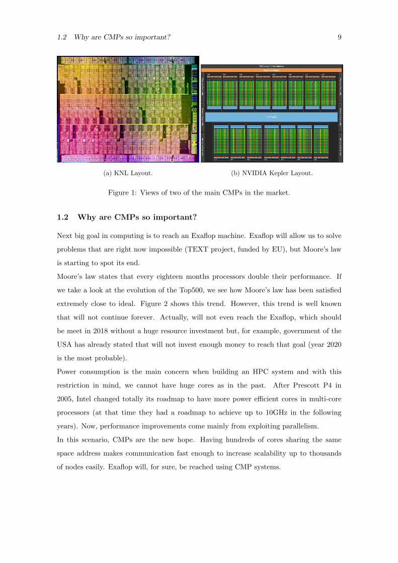
(a) KNL Layout. (b) NVIDIA Kepler Layout.
Figure 1: Views of two of the main CMPs in the market.
1.2 Why are CMPs so important?
Next big goal in computing is to reach an Exaflop machine. Exaflop will allow us to solve
problems that are right now impossible (TEXT project, funded by EU), but Moore’s law
is starting to spot its end.
Moore’s law states that every eighteen months processors double their performance. If
we take a look at the evolution of the Top500, we see how Moore’s law has been satisfied
extremely close to ideal. Figure 2 shows this trend. However, this trend is well known
that will not continue forever. Actually, will not even reach the Exaflop, which should
be meet in 2018 without a huge resource investment but, for example, government of the
USA has already stated that will not invest enough money to reach that goal (year 2020
is the most probable).
Power consumption is the main concern when building an HPC system and with this
restriction in mind, we cannot have huge cores as in the past. After Prescott P4 in
2005, Intel changed totally its roadmap to have more power efficient cores in multi-core
processors (at that time they had a roadmap to achieve up to 10GHz in the following
years). Now, performance improvements come mainly from exploiting parallelism.
In this scenario, CMPs are the new hope. Having hundreds of cores sharing the same
space address makes communication fast enough to increase scalability up to thousands
of nodes easily. Exaflop will, for sure, be reached using CMP systems.

10 1 INTRODUCTION
Figure 2: Performance of the Top500 from the last years.
1.3 Computer architecture simulators
Computer architecture simulators can be classified into many different categories depend-
ing on the context.
• Scope: micro-architecture vs. full-system simulators. The modeled scope could be
only one microprocessor or the whole computer system.
• Detail: functional vs. timing (or performance) simulators. Functional simulators
emphasize achieving the same function as the modeled components (what is done),
while timing simulators strive to accurately reproduce the performance/timing fea-
tures (when is it done) of the targets in addition to their functionalities.
• Input (sometimes called Workload): trace-driven (or event-driven) vs. execution-
driven simulators. Traces/Events are pre-recorded streams of instructions with some
fixed input. Execution-driven simulators allow dynamic change of instructions to be
executed depending on different input data.
Simulators are used in different stages of an integrated circuit design and there are several
different methods or simulator types depending on what we want to measure/validate.
1.3 Computer architecture simulators 11
Usually, in an early stage when path-finding occurs we would probably need functional
simulators that abstract most of the components but give you a rough but fast perfor-
mance estimation.
In later stages, most probably one will need to get more detailed simulations to be able to
debug possible functional or even performance bugs, using timing (cycle-accurate) simu-
lators .
In final stages one will need to validate both functionality and performance numbers. Be-
fore releasing the IC one must be sure that it does exactly what it is supposed to do and
performs how it it supposed to do.
In this project we present a new method to feed a simulator, so we will focus in analyzing
the existing input methods.
1.3.1 Synthetic traffic driven
This is the most basic way to drive a simulation. It does not require any traces or any
executable. It usually injects traffic following a pattern given a few parameters.
For example, if we want to test the maximum bandwidth that our interconnect can pro-
vide, we can create a traffic generator that injects one (or more) memory transaction
per core every cycle, which will eventually collapse the interconnect and will show us the
bandwidth numbers we are looking for.
Synthetic traffic is also useful when trying to characterize a parallel application with thou-
sands of nodes working together. The idea is that the synthetic traffic resembles how nodes
communicate among them in a very general way, for example, when doing barriers or ping
pong communication.
Usually, synthetic traffic generators can be parameterized, for example, continuing with
the interconnect, we can define a % of reads and % of writes, we could also define hit
ratio, etc. However, synthetic traffic is used for very concrete purposes since it does not
show real application traffic, which tends to have heavy variations along execution time.
1.3.2 Execution-driven
The main advantage of using execution-driven simulations is that you can appreciate real
traffic and you can see also how it changes together with the input data to the program.
It represents the most accurate way of injecting traffic to a simulator.
12 1 INTRODUCTION
The main drawback of execution-driven simulations is the runtime. Drive a simulation
using the execution online means that for every event we want to capture there must be
some instrumentation and some extra work, which is a considerable overhead.
For example, Gem5 is a simulator that supports full-system simulation together with
execution-driven. This means that every time an instruction is executed, Gem5 must in-
tercept it, retrieve information, make the corresponding progress in the simulation and
return to the execution of the program. For every single instruction.
For example, CMP$im, a functional cache hierarchy simulator, only intercepts memory
accesses and has an overhead compared to the real execution about 10000x (ten thousand
times slower). If we would like to simulate in the system level, execution-driven is not
suitable; it does not scale well with the number of nodes.
1.3.3 Trace-driven
Traces-driven simulation, opposite to execution-driven, does not need to do any calculation
to feed the simulation since everything was precalculated when the trace was generated.
The main drawbacks of traces are: first, size of the trace can be huge, which would require
a really fast I/O system, otherwise simulation can be slowed down considerably; second,
traces are fixed, i.e., you cannot decide, after generating the trace, to adjust the working
set dynamically, for example.
However, they allow a post-generation analysis to decide to trace and simulate only the
most representative parts of the workload (regions that are the most representative).
13
2 Related work
Trace-driven simulation is not a recent topic. Simulation has been always very useful when
trying to understand applications in order to optimize them.
However, we considered that what has been done up to this moment was not enough for
some reasons. Thus, let us take a look to the existing work to see why it was not enough.
2.1 Dimemas
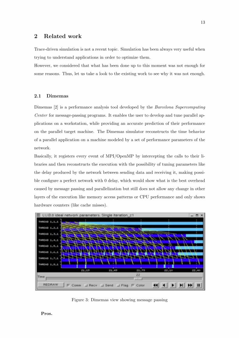
Dimemas [2] is a performance analysis tool developed by the Barcelona Supercomputing
Center for message-passing programs. It enables the user to develop and tune parallel ap-
plications on a workstation, while providing an accurate prediction of their performance
on the parallel target machine. The Dimemas simulator reconstructs the time behavior
of a parallel application on a machine modeled by a set of performance parameters of the
network.
Basically, it registers every event of MPI/OpenMP by intercepting the calls to their li-
braries and then reconstructs the execution with the possibility of tuning parameters like
the delay produced by the network between sending data and receiving it, making possi-
ble configure a perfect network with 0 delay, which would show what is the best overhead
caused by message passing and parallelization but still does not allow any change in other
layers of the execution like memory access patterns or CPU performance and only shows
hardware counters (like cache misses).
Figure 3: Dimemas view showing message passing
Pros.
14 2 RELATED WORK
• Low overhead when generating traces.
• Fast simulation.
• Helps characterizing applications.
Contras.
• Only network parameters can be tuned.
• No notion of other entities other than network. Lack of key components in perfor-
mance studies, like core or memory.
While it is a very useful tool it does not take into account important entities like core
or memory, which we believe are stronger bottlenecks than network most of the times.
However, it can be really helpful when trying to optimize at a different level of abstraction.
2.2 Extended Power Regular Section Descriptors
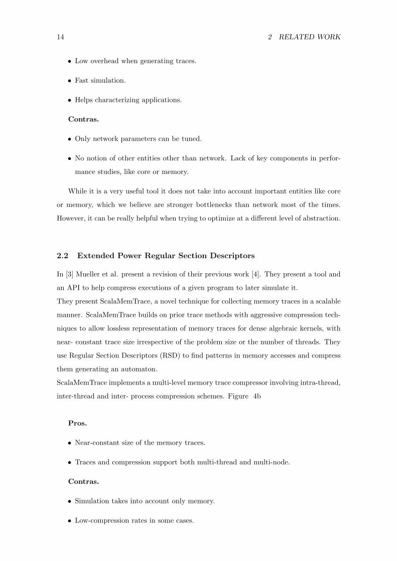
In [3] Mueller et al. present a revision of their previous work [4]. They present a tool and
an API to help compress executions of a given program to later simulate it.
They present ScalaMemTrace, a novel technique for collecting memory traces in a scalable
manner. ScalaMemTrace builds on prior trace methods with aggressive compression tech-
niques to allow lossless representation of memory traces for dense algebraic kernels, with
near- constant trace size irrespective of the problem size or the number of threads. They
use Regular Section Descriptors (RSD) to find patterns in memory accesses and compress
them generating an automaton.
ScalaMemTrace implements a multi-level memory trace compressor involving intra-thread,
inter-thread and inter- process compression schemes. Figure 4b
Pros.
• Near-constant size of the memory traces.
• Traces and compression support both multi-thread and multi-node.
Contras.
• Simulation takes into account only memory.
• Low-compression rates in some cases.

2.2 Extended Power Regular Section Descriptors 15
(a) Dataflow of the compressor (b) Design of the memory trace compressor.
Figure 4: EPRSD compressor view.
• Near-constant size seems to happen when increasing the number of threads, not the
problem size.
This approach has some really good points like being able to find inter-thread and
inter-node patterns, but is still sticking to only referring memory and not the core not
even in an abstract level. Moreover, the compression techniques used are not suitable for
a fast simulation since they require lots of computational power.
16 3 FAST AUTOMATON-DRIVEN SIMULATION
3 Fast Automaton-Driven Simulation
Fast Automaton-Driven Simulation or FADS from now on, is the name of our contribu-
tions.
FADS is based on the idea that an automaton can drive a simulation faster than existing
methods. The most typical, simple and used method to drive simulations are traces.
Trace-driven simulation typically require no computation (to drive the simulation) but
have the disadvantage that require larger I/O systems (traces tend to be big), otherwise
could happen that reading the trace can become slower than make some computation. For
this reason, trace generation need to make a tradeoff between the information available
and the space. Another typical method to drive simulations is binary execution, but this
method require to do all the computation that the benchmark requires plus the simulation;
for example, deciding whether to take or not to take a branch require usually data to be
calculated by software. This method can get really accurate (up to 100%) but can also
get really slow (days to simulate a few millions of cycles).
FADS is a solution in between, it needs to do some calculations but most of it is pre-
calculated (and efficiently compressed). However, since we get a really tiny file, reading it
from disk get negligible and since we have most of the information precalculated we can
get even faster than usual traces (and with way more information to make our simulation
even more accurate).
3.1 Control Flow Graph
Control Flow Graph (CFG from now on) is the name given to the graph describing the
automaton.
The automaton contains all the information needed to reproduce the execution of a given
program.
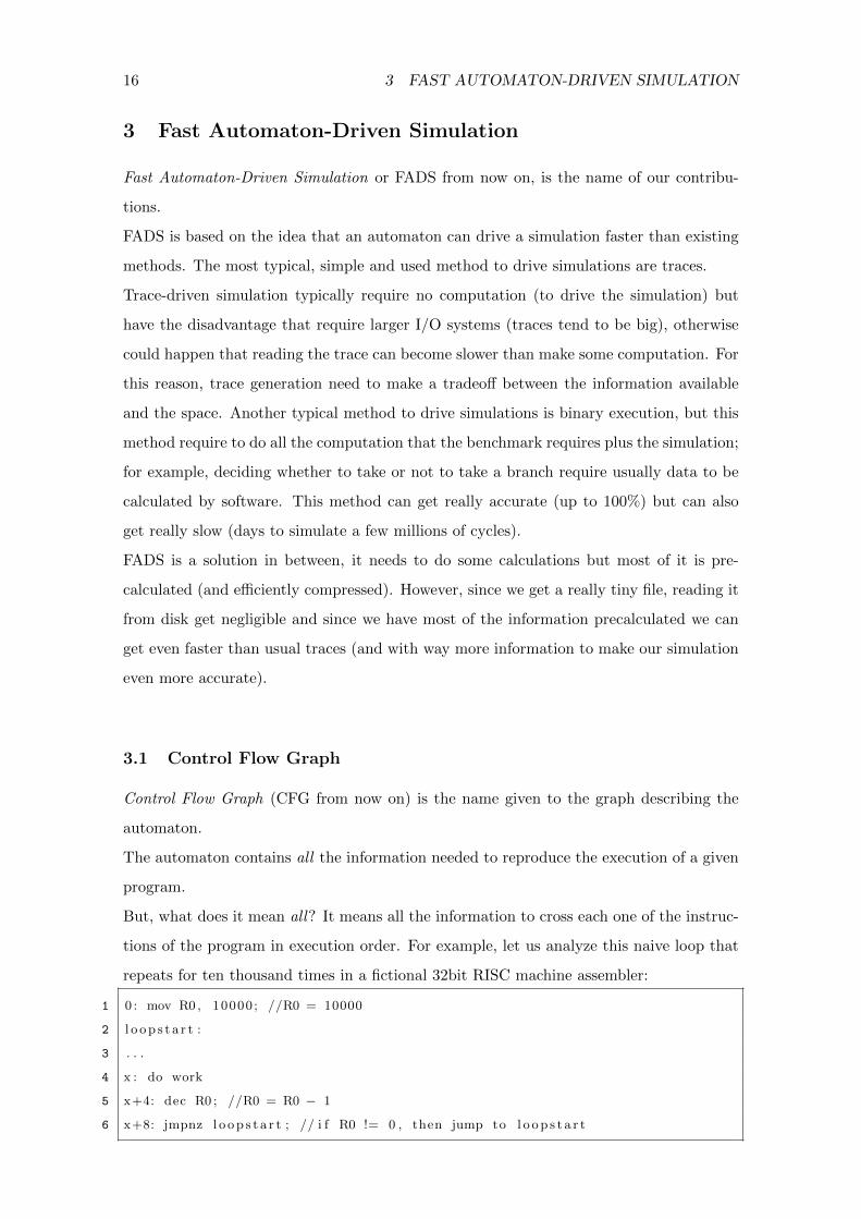
But, what does it mean all? It means all the information to cross each one of the instruc-
tions of the program in execution order. For example, let us analyze this naive loop that
repeats for ten thousand times in a fictional 32bit RISC machine assembler:
1 0 : mov R0 , 10000 ; //R0 = 10000
2 l o op s t a r t :
3 . . .
4 x : do work
5 x+4: dec R0 ; //R0 = R0 − 1
6 x+8: jmpnz l o op s t a r t ; // i f R0 != 0 , then jump to l o op s t a r t

3.1 Control Flow Graph 17
Tracing this tiny snippet with traditional techniques that write the program counter
to know its evolution along time, would require, without any extra work in it, ((10000×
2)+1)instr.*4B/instr. = 80004B 78KB. However, we can encode this in just a few tens
of bytes.
We construct our automaton in a way that each node in it represents a basic block of
the original program execution, with its entry point and its end point. Edges of the au-
tomaton correspond to jumps between basic blocks in the execution, which can be due a
branch/jump, a call/ret, rep prefix (for x86 code) or even just fall through when the next
instruction is a target of a jump or a branch.
But only this information is not enough to reproduce the execution in the same execution
order.
3.1.1 Conditional Branches
In order to reproduce the execution we need to account for anything that can break the
normal execution order of a program.
If we want to take jumps exactly as in the original execution but without any data to
evaluate conditions (that would require way too much computation, is what fully accurate
but slow models do), we need to store if whether a conditional branch was taken or not
or where a jump jumped.
3.1.2 Call Stack
Another event that can break the execution order are call instructions.
Handling call instructions is easy since mostly there is only one call address to a function
(more if it is called through a function pointer) but return instructions are more problem-
atic since every time is called, the return address is potentially different.
We solve this by not storing the return address (as for the call or a jump) but creating
a stack and every time we hit a call instruction we push its return address, which corre-
sponds to the next in the fall through order of the call instruction, and when we hit the
return instruction we pop the return address. During the construction of the automaton
we do the opposite, we push the call instruction and when we hit the return we pop the
call instruction in order to create a link between the call and its return.
Following figure shows this concept graphically:
18 3 FAST AUTOMATON-DRIVEN SIMULATION
3.2 Generating memory traces
Memory traces is the milestone of FADS. We consider memory hierarchy a key element
for performance studies of a node. For this reason all our efforts were put in simulating
as fast and accurate as possible the access to the different levels of memory.
In literature [Citaiton needed] we can find many examples of methods to infer access
patterns (whether to memory, I/O or other entities) but they usually rely on a loss of in-
formation and thus, accuracy. Simple patterns that can only reproduce effects like memory
contention or more complex patterns that can reproduce more accurately part of the exe-
cution (usually where the patterns are more visible).
However, when using an automaton we can find trivially patterns all along the execution,
they almost show up by themselves, and thus we can compress them in a very efficient
manner.
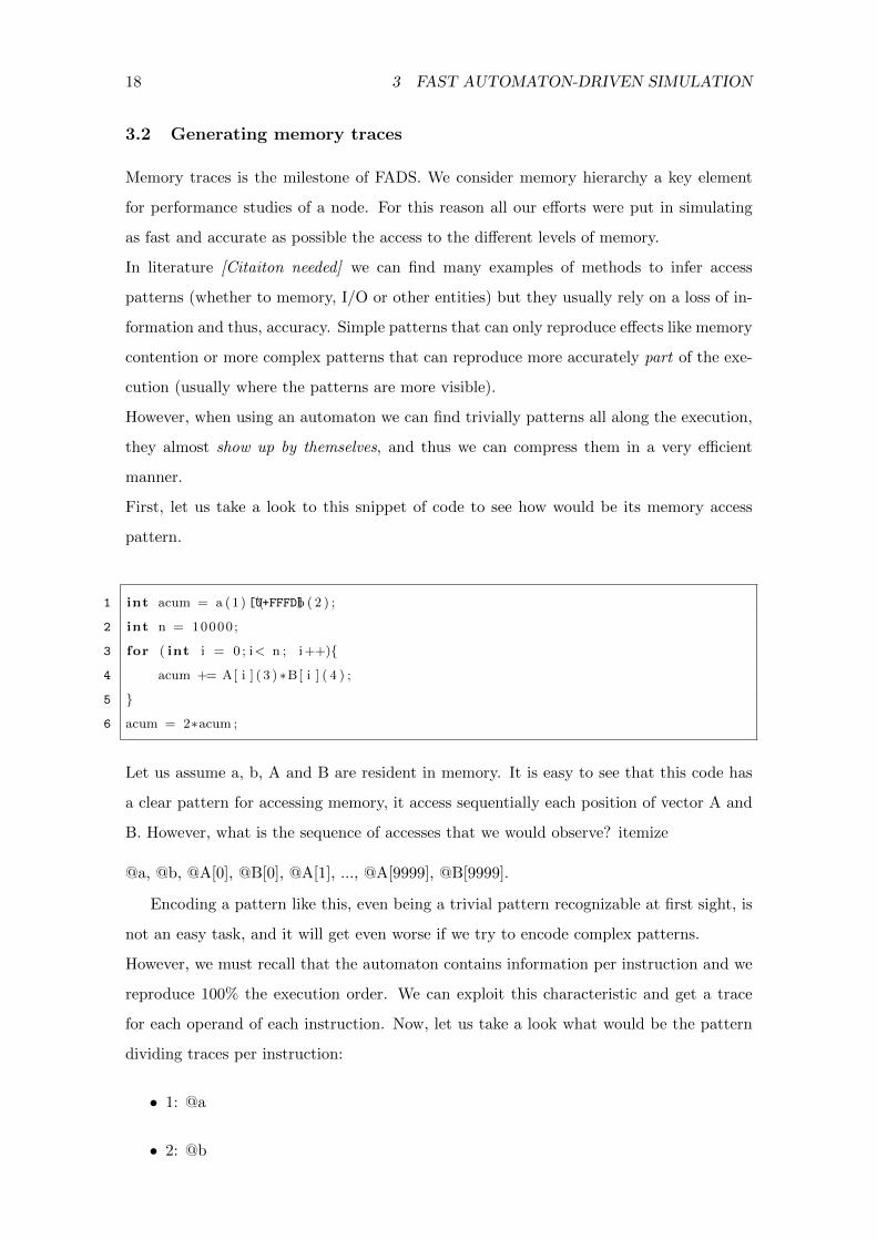
First, let us take a look to this snippet of code to see how would be its memory access
pattern.
1 int acum = a (1) \[U+FFFD]b ( 2 ) ;
2 int n = 10000 ;
3 for ( int i = 0 ; i< n ; i++){
4 acum += A[ i ] ( 3 ) ∗B[ i ] ( 4 ) ;
5 }
6 acum = 2∗acum ;
Let us assume a, b, A and B are resident in memory. It is easy to see that this code has
a clear pattern for accessing memory, it access sequentially each position of vector A and
B. However, what is the sequence of accesses that we would observe? itemize
@a, @b, @A[0], @B[0], @A[1], ..., @A[9999], @B[9999].
Encoding a pattern like this, even being a trivial pattern recognizable at first sight, is
not an easy task, and it will get even worse if we try to encode complex patterns.
However, we must recall that the automaton contains information per instruction and we
reproduce 100% the execution order. We can exploit this characteristic and get a trace
for each operand of each instruction. Now, let us take a look what would be the pattern
dividing traces per instruction:
• 1: @a
• 2: @b
3.2 Generating memory traces 19
• 3: @A[0], @A[1], @A[2], ..., @A[9999]
• 3: @B[0], @B[1], @B[2], ..., @B[9999]
Now the pattern looks trivial, for (3) and (4) it is just the previous address plus a
constant offset, 8B in a 64bit machine.
This clear patterns allow us to use really efficient compression methods. Efficient in com-
pression (good compression ratio) and efficient in decompression (calculation is minimum
and space in memory after decompression is minimal). The algorithm will be explained
in more detailed in 3.3.
20 3 FAST AUTOMATON-DRIVEN SIMULATION
3.3 Trace compression
In the example shown in section 3.2, after storing the memory traces per operand and
instruction, we could see clear patterns, but what is the best to compress this? As it
was previously stated it must be efficient compression (in terms of compression ratio, no
matter compression time since it will be done offline the simulation) and efficient in terms
of decompression (fast enough to not slow down simulation).
3.3.1 Preprocess of traces
Let us return to the previous example in section 3.2. Let us assume also that virtual
address of A and B are 0x40000 and 0x60000 respectively. The memory address sequence
in a 64bit machine would be as follows:
• 3: 0x40000, 0x40008, 0x400010, ..., 0x53878
• 4: 0x60000, 0x60008, 0x600010, ..., 0x73878
Still the same pattern and in the same way, but now, let’s preprocess the traces in
order to get a better compression ratio. What happens if we express addresses in terms
of base address + offset. Traces would resemble this:
• 3: 0x40000, 8, 8, 8, 8, 8, ..., 8
• 4: 0x60000, 8, 8, 8, 8, 8, ..., 8
Having the trace in this form it is trivial to find a compression algorithm that would
meet our requirements (good compression ratio and fast decompression): Run-length en-
coding.
3.3.2 Run-length encoding
Run-length encoding, or RLE, is a very simple algorithm of data compression in which we
have sequences of pairs. Each of this pairs give us a value and the number of times this
value has been repeated consecutively in the original sequence. Using RLE compression
algorithm the previous traces can be compressed in just a few bytes:
• 3: 0x40000, 1, 8, 9999
• 4: 0x60000, 1, 8, 9999
3.3 Trace compression 21
This would meet our requirements of compress ratio but also, decompression is trivial. If
we implement this using a vector of pairs per trace, we just need to have a pointer to the
position of the vector to know which offset are we using in a given moment and another
counter that would tell us how many times have we used it. Moreover, after decompress it,
space in memory does not increase, which is crucial for a fast simulation of large systems
because having constantly page faults is something we need to avoid at all costs.
3.3.3 Principal Component Analysis
When compressing traces, we can go a step further. Patterns not only show inside a trace
as we have seen but also among traces. Let us rescue again the previous traces. Accesses
to A and B are following a simple patter: @B[i] = @A[i] + offset. Then, why not exploit
these similarities?
Principal component analysis (PCA from now on) is a statistical procedure that uses an
orthogonal transformation to convert a set of observations of possibly correlated variables
into a set of values of linearly uncorrelated variables called principal components, i.e., it
allows us to express a trace as a function of another.
However, performing PCA in big sets of data (like all the memory references of an ex-
ecution) is really CPU and time consuming. Thus, instead of performing PCA on each
trace with respect all every other trace, we have decided to do it according to a set of
restriction to minimize the set of possible traces (ideally, without a loss in accuracy). Our
restrictions are:
• We only consider traces with the same size after compressing with RLE. If two
traces have the same size after compressing them using RLE most likely they will
have patterns in common since RLE compression ratio is really dependent on the
patterns (more constant patterns will achieve a higher compress ratio).
• We only consider traces in the same basic block. Similarity inside a basic block is
usually higher than between blocks. Recall our previous example, when compressing
traces A and B.
Thanks to this restrictions we prune the set of possible traces and we do not need years
to compute all the combinations. In reality, this works fairly well since most of the pat-
terns are found in traces in the same basic block and it simplifies also the decompression
algorithm.

22 3 FAST AUTOMATON-DRIVEN SIMULATION
We compute PCA using the covariance method. It is the following:
• Calculate the empirical mean. We get a vector u[1,...,n].
• Calculate the deviations from the mean. We obtain a matrix B, n× p.
• Find the covariance matrix. We obtain a p× p matrix C.
• Find the eigenvectors and eigenvalues of the covariance matrix. We compute the
matrix V of eigenvector which diagonalizes the covariance matrix C: V −1CV D.
Where D is the diagonal matrix of eigenvalues of C. We do this using a mathematical
library.
• Rearrange the eigenvectors and eigenvalues.
• Compute the cumulative energy content for each eigenvector. The cumulative energy
content g for the jth eigenvector is the sum of the energy content across all of the
eigenvalues from 1 through j.
• Select a subset of the eigenvectors as basis vectors. This is the most important step
and the accuracy of our simulations will depend on this step. We have decided to
keep as many eigenvectors as we need so that the cumulative energy g is above the
percentile 99%. Less could lead to inaccuracy when reproducing the memory ac-
cesses. We have found that 99% is enough since we work with integers and rounding
with a potential error of 1% is enough to get the exact original trace and we still
have very good compression ratios as we will see in section 6.2.5.
After computing the component analysis we get as a result an eigenvector, a vector of
eigenvalues, which form the basis for the data.
3.3.4 Binary compression
When compressing with RLE we are only exploiting, first level patterns.
If we have a loop that access sequentially a vector but it is nested inside another loop, we
will not catch the pattern of accessing the vector after the deepest loop finishes.
For example
• A[0], A[1], ..., A[N-1], A[0], A[1], ..., A[N-1], A[0], ..., A[N], which corresponds to a
loop inside another loop always iterating M times sequentially over vector A with

3.3 Trace compression 23
size N.
It will be compressed to a set of pairs instead of only one even having such a clear
pattern. Assuming A is a vector whose elements are 64bits (8B):
• 8, N, 1, -8*N, 8,N, ..., 1, -8*N, 8, N.
While it could be compressed like follows:
• M, 8, N, 1, -8*N.
We could adapt RLE algorithm to find second-level patterns but it is extremely costly
to make it find all levels, so we decided to keep it simple. However, GZIP can be really
helpful when it comes to find this patterns. Binary compression is always an option when
thinking about compressing something: easy to understand and proven to work. However,
it can be very time consuming to decompress, which is the opposite we need for a fast
simulation.
On the other hand, we preprocess traces in such way that usually, it is easier for gzip to
find patterns and also, we have a larger margin when it comes to decide how much effort
we want to put in compression (and thus decompression) since originally our traces after
applying RLE and PCA are already considerably smaller than raw traces.
For this reason, we believe using ZIP binary compression can report high benefits that
overcome its overhead.
3.3.5 Efficient decompression
We are compressing traces for two reasons: space usage, disk is not finite and traces can
get really huge; and for a more efficient simulation, I/O is usually slower than some com-
putation and it is faster to compute memory addresses than reading gigabytes of memory.
However, we need the decompression to be efficient, otherwise we are only compressing
to do room for more traces, but not for speeding up a simulation, which is the main goal
(disk space is cheaper than CPU performance and way cheaper than a designer’s time).
First step in the decompression is the last step in the compression, GZIP. In this step, we
benefit from the feature of GZIP algorithm that allows us to decompress chunk by chunk.
Thus, we do not have to be swapping memory from main memory to disk, since it is really
costly. This is something that a normal trace-driven feeder could also do but the difference
is how much information is contained in the same zipped chunk. While the first will just
get a raw trace, we will obtained a significantly smaller trace still compressed with RLA
and PCA.

24 3 FAST AUTOMATON-DRIVEN SIMULATION
For PCA we have that PCV X, where PC are the Principal Components, X is the matrix
with our trace and V is the matrix with the eigenvectors. To decompress PCA we just
need to perform the following multiplication: XV TPC.
For RLE the decompression is quite trivial. Since all the information is stored in pairs of
offset, repetitions we only need to keep track of where are in the trace using two counters:
the first keeps track of what offset are we using at each moment and the second keeps
track of how many repetitions we have done up to a given moment.

25
4 System level performance projection
The main goal of this project is to be able to simulate efficiently Chip Multi-pprocessors
but a standalone CMP is completely useless, nobody would buy that as with a Desk-
top/Server Processor, where usually are preferable less core count but higher single thread
performance. However, CMPs are meant to be part of a larger system, like a supercom-
puter. For this reason, we should be able to simulate efficiently a system with a large
amount of nodes.
Usually, parallelism is achieved in two ways: OpenMP (shared memory multi-threading)
and MPI (Message Passing Interface). Parallelizing an application is not an easy task,
that is the reason for why we will focus on MPI.
Message Passing Interface (MPI from now on) has become a de facto standard. Widely
used because of its easiness of usage, no need to care about what is being shared and how
this should be protected and accessed and also, it is easy to get a great scalability up to
thousands of nodes (larger scales may need further work).
For all this, we have also implemented support for generating an automaton for also MPI
applications to later reproduce its behavior using another simulator that can simulate a
fabric interconnect (network between different nodes in a supercomputer).
4.1 Adding MPI support to FADS
CFG can reproduce the execution of a program, including memory accesses in a fast and
accurate way, storing all the information we need for it.
Adding support for MPI applications is an easy task once we know how the main idea
behind the automaton works.
CFG store information per basic block. This includes: entry and exit points, jump/branch
info, function address if it ends with a call, memory traces per operand, etc. With this
scheme is easy to add more information and now we just have to intercept MPI calls when
constructing the automaton and put an extra parameter to know when the automaton is
executing a call that is, in fact, an MPI call.
For the moment we have to store the MPI call id and all the parameters of a given call:
receiver, sender, tag of the transaction, etc. However, priority for the future work is to
find a method to infer this information, which would give us the ability to get a trace,
construct one automaton and be able to reproduce an execution with an arbitrary number
of nodes, for example, 100k nodes, like future systems presumably have.

26 4 SYSTEM LEVEL PERFORMANCE PROJECTION
MPI events simulation is simulator-dependent. We provide the information but depend-
ing on the simulator on top to simulate the fabric interconnect, the interface will need to
encapsulate the events to what the simulator understands.
4.2 Iterative simulation
Thanks to the automaton based implementation we can have precalculated information.
The way this information was calculated is not important as long as it is stored when the
current simulation starts.
FADS allows us to reproduce memory accesses. However, when trying to perform a sys-
tem level performance projection this is something really costly (it will not scale with the
number of nodes) and its impact on performance diminishes as the system grows, but
this does not mean that it is not important anymore. What we could do is simulate one
or a few nodes with memory operations enabled and use the results of the simulation to
improve future simulations without having to simulate memory accesses.
The idea behind iterative simulation is to simulate once, obtain some performance num-
bers and tune the automaton with them. This will give more accuracy to the automaton
without compromising runtime or scalability. This process can be done as many times as
desired.
27
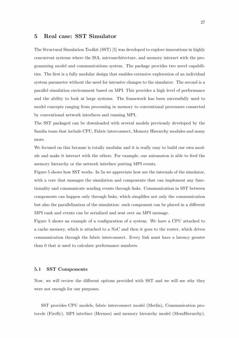
5 Real case: SST Simulator
The Structural Simulation Toolkit (SST) [5] was developed to explore innovations in highly
concurrent systems where the ISA, microarchitecture, and memory interact with the pro-
gramming model and communications system. The package provides two novel capabili-
ties. The first is a fully modular design that enables extensive exploration of an individual
system parameter without the need for intrusive changes to the simulator. The second is a
parallel simulation environment based on MPI. This provides a high level of performance
and the ability to look at large systems. The framework has been successfully used to
model concepts ranging from processing in memory to conventional processors connected
by conventional network interfaces and running MPI.
The SST packaged can be downloaded with several models previously developed by the
Sandia team that include CPU, Fabric interconnect, Memory Hierarchy modules and many
more.
We focused on this because is totally modular and it is really easy to build our own mod-
ule and make it interact with the others. For example, our automaton is able to feed the
memory hierarchy or the network interface putting MPI events.
Figure 5 shows how SST works. In 5a we appreciate how are the internals of the simulator,
with a core that manages the simulation and components that can implement any func-
tionality and communicate sending events through links. Communication in SST between
components can happen only through links, which simplifies not only the communication
but also the parallelization of the simulation: each component can be placed in a different
MPI rank and events can be serialized and sent over an MPI message.
Figure 5 shows an example of a configuration of a system. We have a CPU attached to
a cache memory, which is attached to a NoC and then it goes to the router, which drives
communication through the fabric interconnect. Every link must have a latency greater
than 0 that is used to calculate performance numbers.
5.1 SST Components
Now, we will review the different options provided with SST and we will see why they
were not enough for our purposes.
SST provides CPU models, fabric interconnect model (Merlin), Communication pro-
tocols (Firefly), MPI interface (Hermes) and memory hierarchy model (MemHierarchy).

28 5 REAL CASE: SST SIMULATOR
(a) SST Components (b) SST configuration example
Figure 5: Overview of SST.
This way, we just need to worry to develop a component of a CPU model to try our
automaton in order to feed the simulation in a multi-node system.
We will focus now in the CPU models since are the ones that provide the same func-
tionality and we will do a quick review on them to see why we believe ours is a better
solution.
• Ariel: execution-driven by PIN (an instrumentation tool provided by Intel for x86
architectures). For every instruction it captures memory operations and creates a
memory event that will go to the memory hierarchy module. It also modules a naive
buffer system that can have a parameterized number of requests on the fly.
It has a considerable overhead because of being execution-driven and it is not doing
something special that could not be done by a trace-driven simulation easily (like
performing real computation with real data).
• Prospero: trace-driven with the naive format we showed in previous sections. Only
memory operations and traces just have memory addresses, transaction type (R/W),
transaction size and timestamp.
• Ember: Probably the most interesting one. Ember is a CPU model that works with
motifs. Motifs are tiny modules that emulate the behavior of a parallel application.
It is really fast and scalable but requires time to transform an application to its
motifs counterpart. It is intended to emulate only MPI applications and is useful to
see roughly how a system would behave when running a given type of application.
It can scale easily to more than 100K nodes. However, it requires some previous
work and also is difficult to determine whether it is representative enough to do a

5.2 FADS in SST 29
performance projection of a large system.
In section 6.3 we complement this short description with a further analysis in runtime
and capabilities of each of the solutions.
5.2 FADS in SST
We have developed a component for SST that basically implements FADS and generates
traffic to drive the simulation and feeds different components.
The FADS component traverses the automaton and generates and injects memory events
to the memory hierarchy component. It also is capable of generating MPI events using
Hermes (MPI interface for SST) in a similar way that Ember does.
We have also implemented a feature that allows FADS to generate event traces similar
to Paraver traces that the Dimemas simulator uses. We find this feature really powerful
since it permits to generate tiny traces (less than 10KB/node) that can drive faster a
simulation for parallel applications. When we are dealing with simulations of thousands
of nodes we do not need to simulate, for example, the full memory hierarchy, since it would
make simulation unfeasible and its effect diminishes as the systems grows. However, we
can use information such as CPI or miss ratio for caches and memory for every single basic
block, retrieved from previous simulations (at a node scale, most probably). This would
make our system level simulation way more accurate without compromising performance.
In section 6.3.4 we analyze the performance of FADS in the two formats above mentioned.
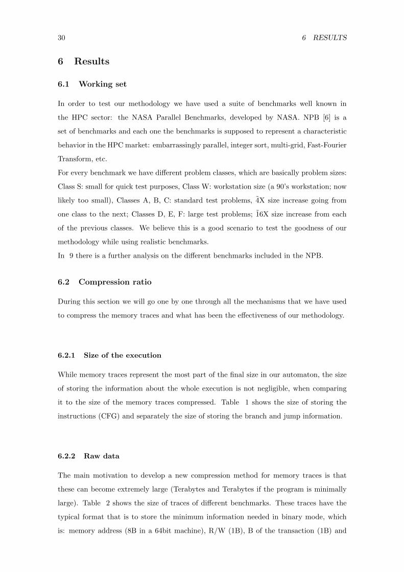
30 6 RESULTS
6 Results
6.1 Working set
In order to test our methodology we have used a suite of benchmarks well known in
the HPC sector: the NASA Parallel Benchmarks, developed by NASA. NPB [6] is a
set of benchmarks and each one the benchmarks is supposed to represent a characteristic
behavior in the HPC market: embarrassingly parallel, integer sort, multi-grid, Fast-Fourier
Transform, etc.
For every benchmark we have different problem classes, which are basically problem sizes:
Class S: small for quick test purposes, Class W: workstation size (a 90’s workstation; now
likely too small), Classes A, B, C: standard test problems, 4X size increase going from
one class to the next; Classes D, E, F: large test problems; 16X size increase from each
of the previous classes. We believe this is a good scenario to test the goodness of our
methodology while using realistic benchmarks.
In 9 there is a further analysis on the different benchmarks included in the NPB.
6.2 Compression ratio
During this section we will go one by one through all the mechanisms that we have used
to compress the memory traces and what has been the effectiveness of our methodology.
6.2.1 Size of the execution
While memory traces represent the most part of the final size in our automaton, the size
of storing the information about the whole execution is not negligible, when comparing
it to the size of the memory traces compressed. Table 1 shows the size of storing the
instructions (CFG) and separately the size of storing the branch and jump information.
6.2.2 Raw data
The main motivation to develop a new compression method for memory traces is that
these can become extremely large (Terabytes and Terabytes if the program is minimally
large). Table 2 shows the size of traces of different benchmarks. These traces have the
typical format that is to store the minimum information needed in binary mode, which
is: memory address (8B in a 64bit machine), R/W (1B), B of the transaction (1B) and

6.2 Compression ratio 31
# of instructions
executed
CFG
(KB)
Branch trace
(KB)
Zipper trace
(KB)
MG.W 1.684.418.801 649 9965 56
MG.A 13.201.685.329 653 77314 251
LU.S 76.506.440 672 412 23
FT 384.124.468 644 2304 27
FT.W 1.604.048.446 651 9967 38
SP.W 114.300.235 688 714 25
Table 1: Size of the automaton for different benchmarks
timestamp (8B).
Size (MB)
LU.S 8.600
MG.S 1.304
SP.S 10.240
FT.S 27.852,8
Table 2: Size of raw traces
As we can appreciate, even for a class S (real execution takes less than a second), we
have really huge memory traces: 28GB for the Fast-Fourier Transform. That is a lot of
space taking into account that I/O systems are the slowest part of a system and that if we
want to run this trace in a multi-node simulation running in a cluster, nodes does not have
that much memory and the transfer I/O goes through network, which makes it even slower.
6.2.3 FADS with raw traces
As we said, our automaton has all the information to reproduce an execution. Thus, when
we store a memory trace we do not need to store per every single access the instruction
that is causing it, whether it is read or write, the number of bytes of the transaction nor the

32 6 RESULTS
timestamp, since all of this comes implicit in the automaton and we obtain this information
when reproducing the execution. For this reason, just storing the memory accesses along
with the automaton saves us a lot of space. Figure 6 shows the compression ratio that
we obtain just for the fact of storing the memory accesses along with the automaton:
Figure 6: Compress ratio
Still, these sizes are not suitable for fast simulations.
6.2.4 Run-length encoding
After obtaining the traces we perform the simple, but effective, RLE. Figure 7 show the
compress ratio of RLE with respect the raw traces in the automaton seen in section 6.2.3.
6.2.5 Principal Component Analysis
We explained how we implement the Principal Component Analysis in section 3.3.3. Even
with all the restrictions set to the set of traces that can be matched, we still have a pretty
good compression ratio. Figure 8 shows us the compression ratios after performing PCA
to the RLE traces.

6.2 Compression ratio 33
Figure 7: Compress ratio of RLE
Figure 8: Compress ratio of PCA
6.2.6 Binary compression
As a final step, we decided to apply binary compression to the preprocessed traces. Con-
cretely we have used Gzip algorithm. Figure 9 shows the compress ratio with respect the
preprocessed trace (RLE and PCA).
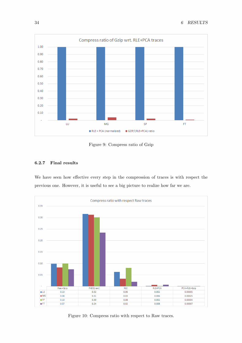
34 6 RESULTS
Figure 9: Compress ratio of Gzip
6.2.7 Final results
We have seen how effective every step in the compression of traces is with respect the
previous one. However, it is useful to see a big picture to realize how far we are.
Figure 10: Compress ratio with respect to Raw traces.
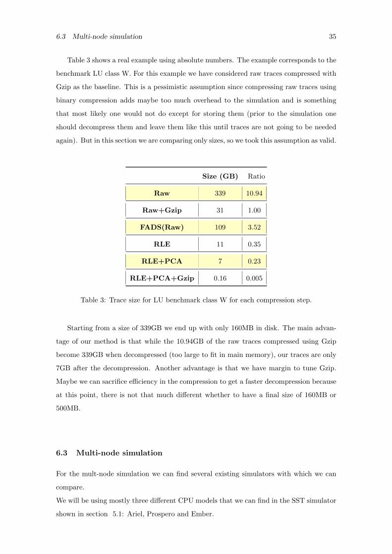
6.3 Multi-node simulation 35
Table 3 shows a real example using absolute numbers. The example corresponds to the
benchmark LU class W. For this example we have considered raw traces compressed with
Gzip as the baseline. This is a pessimistic assumption since compressing raw traces using
binary compression adds maybe too much overhead to the simulation and is something
that most likely one would not do except for storing them (prior to the simulation one
should decompress them and leave them like this until traces are not going to be needed
again). But in this section we are comparing only sizes, so we took this assumption as valid.
Size (GB) Ratio
Raw 339 10.94
Raw+Gzip 31 1.00
FADS(Raw) 109 3.52
RLE 11 0.35
RLE+PCA 7 0.23
RLE+PCA+Gzip 0.16 0.005
Table 3: Trace size for LU benchmark class W for each compression step.
Starting from a size of 339GB we end up with only 160MB in disk. The main advan-
tage of our method is that while the 10.94GB of the raw traces compressed using Gzip
become 339GB when decompressed (too large to fit in main memory), our traces are only
7GB after the decompression. Another advantage is that we have margin to tune Gzip.
Maybe we can sacrifice efficiency in the compression to get a faster decompression because
at this point, there is not that much different whether to have a final size of 160MB or
500MB.
6.3 Multi-node simulation
For the mult-node simulation we can find several existing simulators with which we can
compare.
We will be using mostly three different CPU models that we can find in the SST simulator
shown in section 5.1: Ariel, Prospero and Ember.

36 6 RESULTS
6.3.1 Prospero
Prospero is the naivest CPU models among all we are analyzing. It just read memory
operations out of a trace file. There is no tracing application with which retrieve Prospero
traces provided along with SST, thus we just analyzed the runtime using the only trace
provided: 100MB of trace 5M instructions, there is no information about the what origi-
nal application is but hardly will correspond to a real workload (way too small for HPC).
Figure 11 shows the runtime of a simulation running Prospero attached to two levels of
cache plus main memory. The trace has no multi-thread support but we wanted to test
the scalability of a trace-driven simulation to check whether it is suitable for large system
simulations or not, so nevertheless we decided to emulate a parallel application running
several instances of the same trace, which would be an optimistic runtime since paralleliz-
ing always comes with overhead.
Figure 11: Prospero runtime.
We scaled up to 72 threads, which is what the new to-be-released Intel Xeon Phi has.
As expected, the runtime increases linearly with the number of threads (there is no over-
head from parallelizing). Simulating with 72 threads takes only 80s, which seems quite
fast, but if we want to simulate large systems it would take days, which is not what we
would call fast simulation. We also need to account for the potential overhead of having
to simulate the fabric interconnect, the MPI protocol and a more realistic trace (larger
traces). And all of this, for a fixed trace that does not allow any further configuration.
For all this reasons we believe we can improve this approach.

6.3 Multi-node simulation 37
6.3.2 Ariel
Ariel models a simple CPU but already accounts for some internal details, which makes
it more accurate, and also is capable of running the whole application, which would make
the simulation more representative.
Figure 12 shows the runtime of Ariel simulating the NPB benchmark MG (Multi-Grid)
with class S, the smallest.
Figure 12: Ariel running MG.S runtime.
Figure 13 shows the runtime of Ariel simulating the NPB benchmark MG with class
W.
Figure 13: Ariel running MG.W runtime.
We can appreciate that both, while fast enough, are capable of running several tens

38 6 RESULTS
of threads of a real application with a decent runtime. However, Ariel supports only
OpenMP threads, so we have to account that this simulation is not having any multi-node
communication with its respective overhead.
6.3.3 Ember
Ember is probably the most interesting of the three CPU models analyzed. Ember works
using motifs, which characterize the behavior of a parallel application. It is extremely fast
but does not account for anything other than MPI events. The CPU is modeled as series
of compute events that just sum some delay to the CPU clock.
Motifs reproduce very simple patterns like a barrier, ping pong communication or just a
simple send or receive.
Figure 14 shows the runtime of Ember simulating different Motifs scaling the system size
but only for one iteration (i.e. if the motif is a barrier, performs only one and finishes).
The topology of the fabric is a 3D torus.
Figure 14: Ember runtime scaling system size.
Figure 15 shows the runtime of Ember simulating different Motifs in a system with 64
nodes arranged in an 8x8 mesh connected in a 3D torus. In this case we are scaling the
problem size, i.e. we increase the number of iterations of the simulation.
As we can see in both cases we are in the order of seconds even simulating a 4K nodes

6.3 Multi-node simulation 39
Figure 15: Ember runtime scaling problem size.
system. However, we need to have in mind we are simulating very basic patterns (are they
enough to extrapolate system performance?) and we also need to analyze and characterize
every application we want to simulate in order to simulate it with Ember. We can reach
the first point while solving the second using our FADS approach.
6.3.4 Final results: FADS runtime
In the previous subsections we have seen several approaches to simulate CPU whether as a
standalone model (Prospero and Ariel) or in a multi-node system (Ember and Dimemas).
They are completely different targets and thus the mechanisms we have nowadays are also
totally different. However, our methodology FADS is really versatile and we can use it
anywhere, although in a different form.
Figure 16 shows us the runtime of a simulation driven by FADS, including memory op-
erations and MPI communication events. We can appreciate that the runtime is higher
than for Ariel, but in Ariel we are running OpenMP threads in shared memory (Ariel is
not capable of running MPI applications) and FADS we are running using MPI (FADS is
not capable of running OpenMP threads), which sums an overhead for the communication
over the fabric interconnect. Even with that, seems that an execution-driven simulation
is better when we just want to capture memory accesses.
However, traces are more powerful in the sense that we can do some postprocess and as
explained in section 8 we have some ideas on how to significantly improve performance of
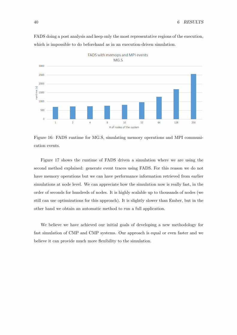
40 6 RESULTS
FADS doing a post analysis and keep only the most representative regions of the execution,
which is impossible to do beforehand as in an execution-driven simulation.
Figure 16: FADS runtime for MG.S, simulating memory operations and MPI communi-
cation events.
Figure 17 shows the runtime of FADS driven a simulation where we are using the
second method explained: generate event traces using FADS. For this reason we do not
have memory operations but we can have performance information retrieved from earlier
simulations at node level. We can appreciate how the simulation now is really fast, in the
order of seconds for hundreds of nodes. It is highly scalable up to thousands of nodes (we
still can use optimizations for this approach). It is slightly slower than Ember, but in the
other hand we obtain an automatic method to run a full application.
We believe we have achieved our initial goals of developing a new methodology for
fast simulation of CMP and CMP systems. Our approach is equal or even faster and we
believe it can provide much more flexibility to the simulation.

41
Figure 17: FADS runtime for MG.S, simulating memory operations and MPI communi-
cation events.
7 Conclusions
We have developed a new methodology to compress memory traces and drive simulations
efficiently.
The main contribution is a new mechanism to find memory access patterns, compress
memory traces lossless and efficiently decompress them.
Our methodology is based on automatons, instead of normal traces and we have seen that
this gives us a powerful tool since automatons can store more information in less space,
can have precalulated information and can also recalculate some other information in case
we want to change some parameters before a simulation in order to try new features.
FADS allows us to drive the simulation of a memory hierarchy simulator, get performance
numbers, generate new traces and later use this information to efficiently drive a new
multi-node simulation without compromising accuracy.

42 8 FUTURE WORK
8 Future work
There are several aspects that we can improve in order to increase efficiency and accuracy
of FADS.
However, there are two features that we would like to implement in the near future:
• Maybe we do not need to simulate and store a whole application. Usually there
are some areas in the timeline of an application that are the most representative
and simulating them could be enough to get a fairly good approximation on the
overall performance of the application. Simpoints [7] is an algorithm that addresses
this problem analyzing some performance counters and determining what are these
areas. This could help to reduce size of the traces but mainly, execution time.
Figure 18 shows an schematic view of this concept.
Figure 18: Simpoints example.
• We have emphasized that the main benefit of using an automaton over a trace or
the execution itself is that precalculated information and information calculated in
runtime can coexist. For this reason we believe we can get to simulate parallel ap-
plications with a fully parameterized number of nodes inferring the characterization
of the parallel communication. We would like to be able to execute the application
in a system with 32 nodes or more than 100K nodes without the need of rerunning

43
the automaton generator.
We also have in mind to try a different approach: probabilistic automaton. This would
increase the compression ratio since would relax the requirements and we could use lossy
compression (we would be fine just having similar patterns compared to the original ex-
ecution). However, this is something that we already tried in the earlier stages of the
project and had to be postponed since it was not as easy as we though in principle. In 10
we explain what we tried.

44 9 APPENDIX A: NAS PARALLEL BENCHMARKS
9 Appendix A: NAS Parallel Benchmarks
In order to validate our methodology we have tried to use representative benchmarks in
the field of HPC. The NAS Parallel Benchmarks (NPB) are a set of benchmarks targeting
performance evaluation of highly parallel supercomputers. They are developed and main-
tained by the NASA Advanced Supercomputing (NAS) Division.
There are other important benchmarks like Linpack, whose performance is used to rank
supercomputers in the Top500 list. However, these benchmarks are designed to be highly
parallel and fully scalable, which does not happen with most of the applications in the
real world.
NPB, on the other side, has different benchmarks and each one targets a different type of
applications. Some are really scalable and some others are not, which is good to test all
different possibilities when trying to do a performance projection for an HPC system.
• MG: MultiGrid. Approximates the solution to a three-dimensional discrete Poisson
equation using the V-cycle multigrid method.
• CG: Conjugate Gradiant. Estimates the smallest eigenvalue of a large sparse sym-
metric positive-definite matrix using the inverse iteration with the conjugate gradient
method as a subroutine for solving systems of linear equations.
• FT: Fast Fourier Transform. Solves a three-dimensional partial differential equation
(PDE) using the fast Fourier transform (FFT).
• IS: Integer Sort. Sorts small integers using the bucket sort.
• EP: Embarrassingly Parallel. Generates independent Gaussian random variates us-
ing the Marsaglia polar method.
• BT: Block Tridiagonal; SP: Scalar Pentagonal; LU: Lower-Upper symmetric Gauss-
Seidel. Solve a synthetic system of nonlinear PDEs using three different algorithms
involving block tridiagonal, scalar pentadiagonal and symmetric successive over-
relaxation (SSOR) solver kernels, respectively. The emphBT benchmark has I/O-
intensive subtype.

45
10 Appendix B: Failed attempts
During the firsts steps of the project, the idea was to build a probabilistic automaton to
drive the simulation, whose data would be obtained from several executions of a given
benchmark and it would be capable of simulating a parameterized execution.
We tried but we had to face major problems difficult to solve and we finally decided to go
in the direction we have seen in this project.
10.1 Probabilistic automaton
Having a probabilistic automaton relaxes the requirements of the compression since it
can be lossy. We are no more working with an exact reproduction of the behavior of an
application but with similar patterns. The main problem we faced when dealing with a
probabilistic automaton to reproduce the whole application is that it is difficult to avoid
taking an incorrect path that would end up simulation too soon or the opposite, it gets
in huge loops. One could think that this is just a matter of running the simulation a lot
of times and in average it would behave as we expect but in reality, execution is big and
it only requires to take one wrong path out of many to get totally different results, which
makes it difficult to trust results. Maybe if we run a sufficiently large amount of times
this would not happen but it would be faster just to run a deterministic solution.
10.2 Problem size parameterizable
Another idea behind building a probabilistic automaton from different executions was to
be able to find a pattern between the execution and the problem size. However, this was
way more difficult than it looked. The idea was to get a polynomial for every edge of
the automaton. We tried using polyfit but then we experienced Runge’s phenomenom [8].
Splines interpolation was clearly not enough neither nor anyother polynomial interpolation
method since some applications’ behavior cannot be determined with a polynomial.
10.3 Clustering
Based on previous work, clustering (K-Means or DBSCAN) seemed like a nice method
to start finding patterns in memory accesses. However, after a few attempts we discov-
ered that just storing a trace per operand the patterns were clearly visible without any
clustering algorithm and that method was even preparing the traces to be later compressed.

46 REFERENCES
References
[1] Top500. Top500 list, June 2014.
[2] Vincent Pillet, Jesus Labarta, Toni Cortes, and Sergi Girona. Paraver: A tool to
visualize and analyze parallel code. In Proceedings of WoTUG-18: Transputer and
occam Developments, volume 44, pages 17–31, 1995.
[3] Sandeep Budanur Frank Mueller and Todd Gamblin. Memory trace compression and
replay for spmd systems using extended prsds.
[4] Michael Noeth, Prasun Ratn, Frank Mueller, Martin Schulz, and Bronis R de Supin-
ski. Scalatrace: Scalable compression and replay of communication traces for high-
performance computing. Journal of Parallel and Distributed Computing, 69(8):696–
710, 2009.
[5] Sandia National Laboratories. Sst simulator.
[6] NASA. Nasa advanced supercomputing division.
[7] Erez Perelman, Greg Hamerly, Michael Van Biesbrouck, Timothy Sherwood, and Brad
Calder. Using simpoint for accurate and efficient simulation. SIGMETRICS Perform.
Eval. Rev., 31(1):318–319, June 2003.
[8] Wikipedia. Runge’s phenomenon.