tracer interpretation using temporal moments on a...
TRANSCRIPT

INL is a U.S. Department of Energy National Laboratory operated by Battelle Energy Alliance
INL/EXT-05-00400
Revision 1
Tracer Interpretation Using Temporal Moments on a Spreadsheet
G. Michael Shook J. Hope Forsmann
September 2005
INL/EXT-05-00400Revision 1
Tracer Interpretation Using Temporal Moments on a Spreadsheet
G. Michael Shook J. Hope Forsmann
September 2005
Idaho National Laboratory Geothermal Technologies Program
Idaho National Laboratory
Idaho Falls, Idaho 83415
Prepared for the U.S. Department of Energy
Assistant Secretary for Energy Efficiency and Renewable Energy Contract DE-AC07-05ID14517

NOTICE
NOTICE: This computer software was prepared by Battelle Energy Alliance, LLC under Contract No. AC07-05ID14517 with the U. S. Department of Energy. The United States Government is granted for itself and others acting on its behalf a nonexclusive, paid-up, irrevocable worldwide license in this software to reproduce, prepare derivative works, and perform publicly and display publicly, by or on behalf of the Government.
Neither the United States nor the United States Department of Energy, nor any of their employees, makes any warranty, express or implied, or assumes any legal liability or responsibility for the accuracy, completeness, or usefulness or any information, apparatus, product, or process disclosed, r represents that its use would not infringe privately owned rights.

iii
ABSTRACT
This report presents a method for interpreting geothermal tracer tests. The method is based on the first temporal moment (mean residence time) of the tracer in the subsurface. The individual steps required to interpret a tracer test are reviewed and discussed. And an example tracer test directs the user through the interpretation method. An Excel spreadsheet application of the interpretation method is a companion document to this report.

iv

v
ACKNOWLEDGMENTS
The authors thank the INL GTP staff for their careful review of the document and Mitch Plummer for sharing his knowledge of Excel tools.

vi

vii
CONTENTS ABSTRACT................................................................................................................................................. iii
ACKNOWLEDGMENTS ............................................................................................................................ v
NOMENCLATURE .................................................................................................................................... ix
1. INTRODUCTION.............................................................................................................................. 1
1.1 Background and Motivation .................................................................................................. 1
2. MOMENT ANALYSIS PROCEDURE............................................................................................. 3
2.1 Correcting for Thermal Decay............................................................................................... 3
2.2 Normalizing the Concentration History ................................................................................ 3
2.3 Deconvolving the Tracer History .......................................................................................... 3
2.4 Extrapolating the History to Long Time................................................................................ 5
2.5 Calculating Mean Residence Times ...................................................................................... 5
2.6 Determining Pore Volume..................................................................................................... 6
2.7 Calculating Flow Geometry .................................................................................................. 6
2.8 Estimating Heterogeneity ...................................................................................................... 7
2.9 Volumetric Fluid Sweep Efficiency ...................................................................................... 8
3. ASSUMPTIONS AND LIMITATIONS............................................................................................ 9
4. EXAMPLE MOMENT ANALYSIS................................................................................................ 10
4.1 Instructions .......................................................................................................................... 10
4.1.1 Step 1................................................................................................................. 10 4.1.2 Step 2................................................................................................................. 11 4.1.3 Step 3................................................................................................................. 13 4.1.4 Step 4................................................................................................................. 14 4.1.5 Step 5................................................................................................................. 14
5. POTENTIAL PROBLEMS AND OBSERVATIONS ..................................................................... 18
6. REFERENCES................................................................................................................................. 19

viii
FIGURES
1. Example of a Raw Data sheet in the TracerAnalysis file....................................................................... 11
2. A portion of Deconv before running the Deconvolution macro ............................................................ 11
3. The Deconv sheet after running the Deconvolution macro ................................................................... 13
4. The original (Eapp) and corrected (Ecorr) tracer histories after running Deconv. ................................ 14
6. A portion of the MoM sheet after running UpdateMoM ............................................................................ 15
7. The F-Φ diagram for the present example ............................................................................................. 16
8. The Sweep Efficiency history for the example problem........................................................................ 16
9. Normalized interstitial velocities for the example problem. .................................................................. 17

ix
NOMENCLATURE
a exponent in the exponential decline equation [=] day-1
b cofficient in the exponential decline equation [=] day-1
C(t) produced tracer concentration [=] parts per billion (ppb)
E(t) age distribution function of a tracer [=] day-1
Ein(t) age distribution function of the injected tracer [=] day-1
Ecorr(t) corrected age distribution function of a tracer (equal to the true E(t)) [=] day-1
Eapp apparent age distribution function of a tracer – equal to true E(t) if no recycling of tracer occurs [=] day-1
floss fluid loss between extraction and injection that leads to increased injection concentrations. Required in deconvolution calculations.
F flow capacity of medium derived from tracer test
m mass of tracer recovered [=] kg
Minj mass of tracer injected in the initial (pulse) injection [=] kg
t time [=] day
tb the time at which onset of exponential decay of the tracer history is observed [=] day
t* first temporal moment of a tracer [=] day
Vp pore volume swept by tracer [=] m3
qinj volumetric injection rate [=] m3/day
δ Dirac delta function
Φ storage capacity of the medium derived from tracer test
ρ density, [=] kg/m3

x

1
Tracer Interpretation Using Temporal Moments on a Spreadsheet
1. INTRODUCTION This document describes a spreadsheet application for tracer test analysis. The analyses are based on
the first temporal moment of a tracer. The governing equations are briefly discussed, and the individual steps required of the user are outlined. A series of Excel macros written in Visual Basic calculate mean residence time, swept pore volume, and flow-storage geometry from a tracer history. The user is directed to the literature cited for more information on the interpretation methodology.
1.1 Background and Motivation The importance of tracer testing is indicated by the more than 100 geothermal tests conducted
worldwide in the last 40 years.a Some workers have used tracer tests to constrain numerical models, using the data to estimate heat transfer parameters (e.g., Robinson and Tester 1984; Axelsson et al. 2001), or to constrain reservoir-scale numerical models (e.g., Gunderson et al. 2002; Bloomfield et al. 2003). However, the vast majority of these tests were interpreted qualitatively, ignoring the temporal evolution of the tracer breakthrough curve and resulting in gross test interpretation (e.g., size of the arrow indicative of relative tracer flow). This document discusses a means of extracting useful, quantitative information from tracer testing.
A host of tracer test analysis methods consider the temporal behavior of tracers. The methods were originally developed for closed reactor vessels (Danckwerts 1958; Levenspiel 1972), but have been applied to more general conditions of open boundaries (Pope et al. 1994), characterization of fractured media under continuous tracer reinjection (Robinson and Tester 1984), and estimates of flow geometry (Shook 2003). These methods have a rigorous mathematical basis and offer additional information about the subsurface. The analysis is useful independently, but also can be used to constrain numerical models by defining interwell volume and flow geometry.
The methods and applications mentioned above are all based on analysis of tracer residence times. The mean residence time, or first temporal moment, is the most useful single property derived from a tracer test, although other properties have been used as well. Levenspiel (1972) shows the total pore volume swept by a tracer can be determined from its mean residence time. Certain restrictions are inherent in the calculation; for example, steady state conditions and conservative tracer behavior. Nevertheless, the method has a rigorous mathematical basis and has been extensively validated analytically and experimentally. The governing equations used in moment analysis are as follows. Terms are defined in the Nomenclature.
∫
∫∞
∞
=
0
0*
dt)t(E
tdt)t(Et (1a)
*qtMmV
injp = (1b)
a M. Adams, University of Utah, personal communication.

2
The means by which individual terms in these equations are estimated from tracer analysis are discussed in the following sections. This discussion is somewhat brief, since the literature cited addresses the method in great detail. The second part of this document summarizes the individual steps required of a user to perform the interpretation using this spreadsheet application, and includes an example analysis.

3
2. MOMENT ANALYSIS PROCEDURE The steps required for accurate tracer analysis are summarized as follows:
• Correct the tracer recovery for thermal decay • Normalize the tracer history • Deconvolve the output signal • Extrapolate the history to late time • Calculate mean residence time and swept volume • Calculate flow geometry.
2.1 Correcting for Thermal Decay Correcting the tracer history for thermal decay is done by applying the Arrhenius equation
(Levenspiel 1972). This is considerably more difficult than the present literature suggests (e.g., Rose et al. 2001), because the decay constant, k, is a function of the temperature. Because the temperature profile of the subsurface is generally not known accurately, proper correction is difficult. This problem has been considered by several authors (e.g., Robinson and Tester 1988), and remains a focus of the Idaho National Laboratory (INL) Geothermal Technologies Program. In this version of the TracerAnalysis spreadsheet, thermal corrections are assumed done a priori by the user.
2.2 Normalizing the Concentration History The method of moments is based on age distribution functions as originally described by Danckwerts
(1953). To avoid ambiguity in terminology, however, we will use the nomenclature of Levenspiel (1972). The age distribution function is referred to as E(t), and has units of (1/t). Tracer concentrations, C(t), are typically reported on a volume or mass fraction basis. Conversion to E(t) is straightforward in either case, though care should be taken to obtain a consistent set of units (e.g., time in days, E(t) in days-1). In the case of volume (mass) fractions, multiply by the volumetric (mass) injection rate, qinj (ρq), and divide by the total mass of tracer injected in the original pulse injection, Minj:
inj
inj
Mq)t(C
)t(E = for C in volume fraction (2a)
inj
inj
Mq)t(C
)t(Eρ
= for mass fraction . (2b)
Working with E(t) instead of C(t) has several advantages. In many applications tracer is reinjected, so the output signal is a combined response to the original pulse injection plus recirculation. Moment analysis is based on analysis of a pulse injection, so the effect of recirculation must first be removed from the output signal. Converting C(t) to E(t) accommodates treating the input signal as a Dirac delta function, the properties of which are required to deconvolve the tracer history, as discussed in the following section. The area under the curve E(t) versus t is unity in a closed system (100% tracer recovery), so the normalized curve offers a quick means of evaluating the flow system.
2.3 Deconvolving the Tracer History When tracer is reinjected, the observed tracer history is a combined response to the initial slug tracer
injection and continuous recycling of the produced tracer. Moment analysis is based on the response to slug tracer injection, so we must first remove the effect of tracer recycling before calculating residence

4
times and swept volumes. The convolution integral is used to deconvolve the tracer response (Levenspiel 1972):
∫ τττ−=t
0inapp d)(E)t(E)t(E (3)
Equation (3) states that the observed (apparent) residence time distribution, Eapp(t), is a result of injection, Ein, and the true residence time distribution, E(t). Following the derivation presented by Robinson and Tester (1984), the terms in Equation (3) can be defined as
inj
injapp M
q)t(C)t(E
ρ= (4a)
inj
inj
lossin M
q)t(Cf11)t(E
ρ⋅
−+δ= . (4b)
Substituting Equation (4b) in Equation (3) gives
∫ ττ⎪⎭
⎪⎬⎫
⎪⎩
⎪⎨⎧ ρτ−
⋅−
+δ=t
0 inj
inj
lossapp d)(E
Mq)t(C
f11)t()t(E . (5)
Applying the delta function on [0,t] and rearranging Equation (5) give the correction needed to
remove the effects of reinjection:
∫ τττ−−
−=t
0in
lossapp d)(E)t(E
f11)t(E)t(E . (6)
The integral in Equation (6) must be calculated anew at each time, using the current tracer
concentration, C(t), the previous injection history, C(t-τ), and residence time ages, E(τ). At the upper limit of the integration, the argument is zero, so the current residence age, E(t), can be calculated explicitly at each time step. Because the initial pulse tracer injection is treated as a Dirac delta function, it is not included in the injection age distribution, Ein.
Equation (6) has been approximated in the spreadsheet discretely at each time step. For example, the corrected age distribution at time step k is given as
t)ik(E)i(Ef11)k(E)k(E
1k
1icorrin
lossappcorr ∆⋅−⋅
−−= ∑
−
=
. (7)
There is currently no provision for a variable time interval in the calculation given above, since E(t) would then have to be interpolated (using a trapazoid rule, for example), and execution speed would degrade. If the tracer signal requires deconvolution, the user is currently required to input tracer histories at constant time intervals. Tracer histories are not usually reported in such a fashion, so the user must interpolate the data before using this spreadsheet. There are a host of free, downloadable software packages to interpolate real data to fixed time intervals.
Exception: If tracer is not reinjected, and if the injection time is much smaller than the residence time (so it can be treated as a Dirac delta function), no correction to the tracer history is required. In that case, the requirement of constant time step size is relaxed. No

5
error is introduced by the deconvolution if no tracer is reinjected, since Ein is identically zero for all times, and the correction is therefore zero as well.
In summary, if tracer is recycled, or if the tracer injection time (frequently referred to as the slug
size, ts) is not small relative to the residence time (ts « t*), the apparent residence time distribution requires correction. The deconvolution integral as implemented [Equation (7)] requires a constant time step size, and so the user must interpolate the actual data. If no deconvolution is required, Ein must be input as zero for all times, and a variable time step is allowed. Deconvolution is still performed in the worksheet, with no ill effects: the correction is identically zero at all times.
2.4 Extrapolating the History to Long Time Sampling for tracer is frequently terminated long before the tracer concentration is zero. Because the
first moment is a time-weighted average, failure to include late time data leads to underprediction of both mean residence time and pore volume estimates [see Equation (1)]. This is addressed by writing Equation (1a) as
∫ ∫
∫ ∫
∫
∫∞
∞
∞
∞
+
+
==b
b
b
b
t
0 t
t
0 t
0
0*
dt)t(Edt)t(E
tdt)t(Etdt)t(E
dt)t(E
tdt)t(Et . (8)
If a curve is fit through the late time tracer data, the second integral in the numerator and
denominator can be evaluated in closed form. For example, if the plot of log(E) versus time is linear for some time t > tb, the decline is exponential, and the tracer data can be written as
atbe)t(E −= for t > tb . (9)
Exponential decline is probably the most common tracer decline observed, perhaps because permeability frequently approximates a log-normal distribution. Other curve types may be used, but only with caution. For example, Shook (2005) showed a tracer test analysis that attempted to apply three different curves to the late time data. The linear curve fit gave non-physical results, and a power law fit gave implausible results; only the exponential fit gave a realistic match over all of the late time data. Because exponential decline is most commonly observed, it is the only option included in the spreadsheet for extrapolation. Symbolic integration of Equation (9) shows
)at1(eabtdt)t(E b
at2
t
b
b
+= −∞
∫ (10)
and
b
b
at
t
eabdt)t(E −
∞
=∫ . (11)
2.5 Calculating Mean Residence Times The mean residence time, or first temporal moment, of a tracer is determined directly from the
normalized, deconvolved, extrapolated tracer history as

6
b
b
b
b
att
0
bat
2
t
0
eabdt)t(E
)at1(eabtdt)t(E
*t−
−
+
++=
∫
∫ . (12)
The integrals in Equation (12) are approximated as sums in the spreadsheet. The constants a, b, and tb are determined by curve-fitting late time tracer data in a spreadsheet macro, described below.
2.6 Determining Pore Volume Pore volume estimates follow directly from the mean residence time (Levenspiel 1972). For open
boundaries, multiple production wells, and/or incomplete recovery of injected tracer, the pore volume swept by the tracer is given as (Pope et al. 1994)
*inj
injp tq
MmV = . (13)
The fractional recovery of tracer at any given well, m/Minj, is the integral of E(t)dt for a given well. In addition to its required use in determining pore volume swept, it is a useful tool for understanding the capture zone of a given well, or degree of openness of flow boundaries. For example, if the sum of all wells’ m/Minj is unity, the system is completely closed.
2.7 Calculating Flow Geometry Shook (2003) shows that the flow and storage (pore volume) geometry of a formation (fractured or
otherwise) can be estimated directly from a tracer test. Individual flow paths are imagined as streamlines that have unique values of permeability, porosity, cross sectional area, and length. The flow capacity, fi, of the individual streamline follows directly from Darcy’s law. By arranging these streamlines in order of decreasing volumetric capacity, we can define a cumulative flow capacity, Fi, at any streamline i as the sum of all streamlines whose velocity is greater than i, normalized by the ensemble properties. The cumulative storage capacity, Φi, of those streamlines is simply the sum of their individual pore volumes.
∑
∑=Φ
=
=N
1jj
i
1jj
iVp
Vp . (14a)
∑
∑=
=
=
N
1j j
jj
i
1j j
jj
i Ak
Ak
F . (14b)
These can be estimated from a tracer test, as follows. The storage capacity, Φ, is the incremental
first moment estimated at time=t, normalized by the true first moment. From Equation 1a, this is written as
7
∫ τττ
∫ τττ=
∫ ττ
∫
∫ ττ
∫ τττ
≅Φ∞∞
∞
∞
∞
0
t
0
0
0
0
t
0
d)(E
d)(E
d)(E
tdt)t(E
d)(E
d)(E
)t( . (15a)
The flow capacity is simply the cumulative tracer recovery at time=t normalized by the complete
recovery.
∫
∫∞
ττ≅
0
t
0
dt)t(E
d)(E)t(F . (15b)
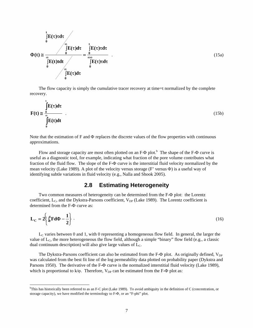
Note that the estimation of F and Φ replaces the discrete values of the flow properties with continuous approximations.
Flow and storage capacity are most often plotted on an F⋅Φ plot.b The shape of the F-Φ curve is useful as a diagnostic tool, for example, indicating what fraction of the pore volume contributes what fraction of the fluid flow. The slope of the F-Φ curve is the interstitial fluid velocity normalized by the mean velocity (Lake 1989). A plot of the velocity versus storage (F’ versus Φ) is a useful way of identifying subtle variations in fluid velocity (e.g., Nalla and Shook 2005).
2.8 Estimating Heterogeneity Two common measures of heterogeneity can be determined from the F-Φ plot: the Lorentz
coefficient, LC, and the Dykstra-Parsons coefficient, VDP (Lake 1989). The Lorentz coefficient is determined from the F-Φ curve as:
⎭⎬⎫
⎩⎨⎧∫ −Φ= 10C 2
1Fd2L . (16)
LC varies between 0 and 1, with 0 representing a homogeneous flow field. In general, the larger the
value of LC, the more heterogeneous the flow field, although a simple “binary” flow field (e.g., a classic dual continuum description) will also give large values of LC.
The Dykstra-Parsons coefficient can also be estimated from the F-Φ plot. As originally defined, VDP was calculated from the best fit line of the log permeability data plotted on probability paper (Dykstra and Parsons 1950). The derivative of the F-Φ curve is the normalized interstitial fluid velocity (Lake 1989), which is proportional to k/ϕ. Therefore, VDP can be estimated from the F-Φ plot as:
bThis has historically been referred to as an F-C plot (Lake 1989). To avoid ambiguity in the definition of C (concentration, or storage capacity), we have modified the terminology to F-Φ, or an “F-phi” plot.

8
5.0
841.05.0DP 'F
'F'FV
=Φ
=Φ=Φ−
= . (17)
F’ is the derivative of the F-Φ plot at the mean (Φ = 0.5) and 1 standard deviation below the mean
(Φ = 0.841). Neither LC nor VDP depends on the form of distribution in heterogeneity, and neither is necessarily unique. That is, different F-Φ curves can yield the same value for LC or VDP, depending on the distribution (Jensen et al. 2000).
2.9 Volumetric Fluid Sweep Efficiency Volumetric fluid sweep efficiency, EV, (as opposed to thermal sweep efficiency) is a measure of
efficiency in the use of injected fluid. It can be defined as the ratio of volume of reservoir contacted by injected fluid to the total pore volume of the reservoir. In case of immiscible fluids present, the definition is modified to account for residual saturations [see Lake (1989) for definitions]. EV is a function of time, heterogeneity, well pattern, and mobility ratio (Dyes et al. 1954).
Using the concept of streamlines and the definition of F above, we can estimate sweep efficiency directly from a tracer test. F(t) can be interpreted as the fraction of streamlines that have “broken through” and begun producing injected fluid. Clearly, those streamlines are not contributing further to sweeping the reservoir. Sweep efficiency, then, can be defined as (volume of fluid injected) * (1 – fraction of streamlines broken through), in dimensionless units. Because injection and extraction rates are potentially different (if, for example, there are multiple production wells), sweep efficiency is written in terms of fractional tracer recovered and injection rates, similar to pore volume calculations [(Equation 13)]:
[ ])tt(F1tM
mVq
)t(E)tt(Einjp
injVV ∆+−∆+=∆+ . (18)
Sweep efficiency is typically reported as a function of dimensionless time, or time normalized by the total pore volume:
*injp
injD t
ttM
mVq
t =⋅⋅= . (19)
Sweep efficiency is frequently plotted as a sweep efficiency history (EV versus tD).

9
3. ASSUMPTIONS AND LIMITATIONS Moment analysis is a general interpretation method, and one that suffers from few limitations.
Assumed conditions essentially state that the flow field is steady and the tracer moves with bulk fluid flow such that the information obtained from the analysis is generally applicable. That is, it does not rely on the specific time the test was run. These conditions can be stated as follows.
1. Steady state injection and extraction
If the flow field is transient, the streamlines are likewise transient and swept volumes, flow geometry, etc., are functions of time. For that reason, a steady flow field is most frequently introduced before conducting the tracer test. Numerical modeling is a useful means of determining the duration of “pretest injection” required to establish steady state flow.
Small (less than 20%) excursions from a constant injection rate can be treated by including the variable flow rate in the normalization of the concentration history [Equation (2)]. The user should recognize variations in flow rate do change the flow field and streamline lengths, velocities, etc., and therefore should consider the analysis in that light.
2. The tracer(s) is ideal and conservative.
That is, it is negligibly soluble in all phases except one (including adsorption on the solid phase) and does not affect flow properties (density, viscosity, etc.). The tracer must also be stable, or degrade in a known fashion (e.g., a radioactive tracer). Theoretically, decay can be corrected for, but in practice the same concerns exist as noted above in correcting for thermal decay: the distribution of the cause is generally not known, and so the correction is unconstrained.
Where multiple phases exist, a conservative tracer test only yields information on the phase in which it exists (e.g., the product of pore volume and average liquid saturation). Partitioning tracers have been used extensively in the environmental field to estimate phase saturations, referred to as partitioning interwell tracer tests (PITTs). PITT analysis is likewise based on first moments of conservative and partitioning tracers, and this spreadsheet could be modified to analyze PITTs. The interested reader is referred to Jin et al. (1995) and Sinha et al. (2004) for further information.
3. The spatial distribution of flow properties is not obtainable from tracer testing.
While pore volume calculations and flow geometry (F-Φ) estimates from tracer tests are robust, the analysis cannot determine the specific location of the flow path distribution. Furthermore, estimates of flow geometry, etc., are volume-averaged (or streamline-integrated) properties; point values cannot be determined uniquely.
In cases where spatial distribution is important, it is likely tracer analysis must be combined with geophysics and inverted jointly to further constrain the problem. That remains an integral portion of the INL Geothermal Technologies Program focus.

10
4. EXAMPLE MOMENT ANALYSIS
An example tracer test analysis is included with this document. The example is synthetic in nature: a tracer test was simulated and the tracer history recorded and analyzed. The domain in this case is a simple rectangle, with two boundaries open to flow, and two closed. Injection occurs in one corner, and two extraction wells are near the diagonally opposite corner. Total production is twice the injection rate (250.5 kg/hr from each of the two producers). At t=0, 60 kg of a conservative tracer is injected, and all tracer mass that is recovered is subsequently reinjected in the next time step. The tracer test was arbitrarily terminated at 500 days. In the steps described below, the analysis is performed for well P1. When the file TracerAnalysis.xls is opened, the only data that appear are in the first sheet, titled RawData. The process of building the other sheets and executing the tracer analysis is given in the steps below.
4.1 Instructions 4.1.1 Step 1
The first sheet in the program is RawData. The user imports the data (time, concentrations, etc.) here, and uses it as a scratch sheet. For example, all well histories can be included here, though only one production well can be evaluated at a time in the subsequent sheets (and those sheets would need to either be Saved under a new filename or Copied within the existing file and renamed). Tracer concentrations are reported in a variety of different units (ppb, vol%, etc.); independent of how the data is reported, it must be converted into a Residence Time Distribution (RTD), E(t). Units for E(t) are in time-1; in this particular example, time is reported in days, so E(t) has units of day.-1
In this example sheet, C(t) has been imported from a field file in units of parts per billion (ppb). C(t) is converted to E(t) by multiplying by the mass flow rate, ρqinj and dividing by the total mass, Minj, of tracer injected in the initial slug:
inj9
inj
M10q)t(C24
)t(Eρ⋅
= .
The constants in this equation are for units’ conversion: mass flow rate in T/hr to T/day, and concentration in ppb to kg/109kg. This conversion must be done for all wells, including injection wells, for reasons discussed below. These are referred to in the spreadsheet as Eapp for the production wells, and Ein for the injection well. Figure 1 shows a portion of the RawData sheet for this example. Note the calculation window showing the conversion from C(t) in ppb to E(t).
In what follows, a single production well and injection well are copied to the next sheet (Deconv), and the balance of the interpretation works on only those two wells. Where more than one production well exists, or tracer is introduced to more than one injection well, this analysis would have to be saved prior to updating the Deconv sheet with a second production well’s E(t). Alternatively, the individual sheets could be copied and renamed within the existing file.

11
Figure 1. A Raw Data sheet in the TracerAnalysis file. Time and tracer concentrations are entered for each well, including the injector, and tracer concentrations are converted to residence time distributions, E(t).
4.1.2 Step 2 The user copies the values of Time, Eapp, and Ein from the Raw Data sheet into the Deconv sheet in
columns A, C, and F, respectively, as shown in Figure 2 below. The cells in yellow are cells the user, as a rule, will input data into. In addition to the three columns mentioned above, required field data are described in Columns M and N. These are discussed below, along with variables that are calculated from the field data.
Figure 2. A portion of Deconv before running the Deconvolution macro. Time, Eapp, and Ein have been copied from the RawData sheet, and field data have been entered in Column N.

12
mdot The mass flow rate of the injector. Units are M/t. Mass flow rates are most frequently used in geothermal engineering (the DOE program that funded this work). It is the product of the volumetric injection rate (required for the moment analysis) and the injected fluid density. These data are not used except to determine the volumetric flow rate, q. In the example provided, the mass flow rate is 0.2505 T/hr (250.5 kg/hr).
Minj
The total amount of mass of tracer injected in the original pulse injection. Units are M (e.g., tonne). In the example, 0.06 T of tracer were injected in the initial slug (60 kg).
∆t The constant time step size of the test analysis. The deconvolution step discussed below requires the interval between tracer samples to be uniform. A constant time step of 1 day was used in the example. If data were reported at unequal time intervals (as is often the case), the user is required to interpolate the data to constant time steps. In the case of no tracer recycling, the restriction of a constant time step is relaxed. The Deconv macro will allow a variable time step only if Ein is identically zero for all times reported.
Fluid loss This variable is needed to calculate the correct injection values, Ein, when tracer reinjection occurs; that is, when the produced fluids are subsequently reinjected. Under certain conditions, some of the produced fluids are lost (e.g., to evaporative cooling), thus concentrating the tracer in less fluid:
)t(Cf11C
lossin ⋅
−= .
Ein is determined as described above from Cin. If the true injected concentration is known, floss can be set to zero and Ein determined explicitly. Fluid loss in the example is 0.
ρ Fluid density. This is used (with mdot above) to calculate volumetric flow rate only. The injected fluid density in the example is 958 kg/m3 – approximately the density of water at 100ºC.
Calc’d Vol Rate Volumetric flow rate calculated from mdot and density. If the user knows q, mdot and density need not be entered (or a 0 entered).
Input Vol Rate In cases where the actual volumetric injection rate is known, as opposed to the mass flow rate, that value can be entered here. The macro will use the larger of the two values of volumetric flow: one from input mass flow rate and density, the other as entered in N7 on the Deconv sheet. For that reason, one or the other of mdot or Input Vol Rate should be entered as 0.
Max Data Rows Equal to or greater than the number of rows of data in the tracer test. The macros will only operate on this many rows. In order to speed up execution time, this number should be close to the actual number of data. No damage is done if this is not true. For example, in the current example, Max Data Rows is 550, yet the number of data is 501. The macros simply take longer than necessary to run.

13
Volumetric Rate Used The greater of N6 and N7. This is the rate actually used in the macros.
After these values are entered in the Deconv sheet, reinjection effects are removed from the tracer output signal. This uses the convolution integral discussed. As noted, if Ein is not identically zero for all time, the time step must be constant and equal to that given in cell N3. If that condition is not satisfied, the macro reports a fatal error and stops. If Ein is zero, variable time steps are allowed.
The deconvolution macro is invoked by typing (ctrl d) from anywhere in the Deconv sheet, or by clicking on the button on the sheet. Column D is calculated as the corrected E(t) from Eapp and Ein. Columns A and D are then automatically copied to Columns A and B of the MoM sheet, and the two plot sheets, Well History, and ExponDecay are updated. Figures 3 and 4 show some results from the Deconvolution macro. Figure 3 is the Deconv sheet with Ecorr filled in (Column D). Figure 4 shows the tracer history plotted on a semilog plot. This tracer history is used in the next step (extrapolating the tracer tail).
Figure 3. The Deconv sheet after running the Deconvolution macro. Ecorr has been calculated by the Deconv macro and is written to Column D. Note that at small times the correction is zero (Ecorr = Eapp), but at late times they differ (rows 17–130 hidden to show both time periods).
4.1.3 Step 3 Extrapolating the tracer tail. The user is directed to the ExponDecay sheet. The user must first
determine the time at which this plot appears linear by using the scroll button to move a data point along the tracer history. When the plot appears linear, the Exponential Trend macro is invoked by typing (ctrl e) or clicking the button. The macro fits an exponential curve through the data for time equal to and greater than that selected by the user, prints the equation and correlation cofficient on the plot, and writes the extrapolation variables required in the moment calculations [Equation (12)] to the MoM sheet.

14
An example of the results from the Exponential Trend macro is given in Figure 5. The user can run this macro until satisfied with the correlation coefficient; the exponential decline parameters (tb, a, and b) are automatically written to the MoM sheet each time it is run. The values obtained in this example are tb = 181 day a = 0.014248 d-1 b = 0.0065 d-1 .
Figure 4. The original (Eapp) and corrected (Ecorr) tracer histories after running Deconv.
4.1.4 Step 4 The moment analysis can then be performed by clicking on the UpdateMom Button (or ctrl u) from
within the MoM sheet. This automatically calculates the first moment and total swept pore volume, and flow and storage geometry, F and Φ. The calculations for t* involve numerical integration of the data for t < tb and symbolic integration for t > tb. These are referred to in the spreadsheet as num (denom), 1/2 for t< tb, and num (denom) 2/2 for t> tb. The flow/storage geometries are plotted in the F-Φ sheet. For reference, a diagonal line (representing homogeneous flow) is also plotted. The Lorentz coefficient and the Dykstra-Parsons coefficient are calculated from the F-Φ data and also plotted on the F-Φ plot. Examples of these sheets are shown in Figures 6 and 7 below.
4.1.5 Step 5 Sweep efficiency can be determined from the interpretations completed thus far. The calculation is
invoked by clicking the Calculate Sweep Efficiency button on the Sweep sheet. A sweep efficiency history (EV versus tD as determined from Equations 18 and 19 above) is plotted, as is the derivative plot dF/dΦ. They are shown for the present example in Figures 8 and 9 below.

15
Figure 5. ExponDecay plot after running ExponentialDecay. The data point (at t=181 days) was moved through the data by clicking the down arrow. When the plot appeared linear, the macro was invoked by clicking on the macro button. The curve fit parameters tb, a, and b are autocopied to the MoM sheet.
Figure 6. A portion of the MoM sheet after running UpdateMoM. Num 1/2 and denom 1/2 are the portions of the moment analysis estimated from the integrals; num 2/2 and denom 2/2 are the extrapolated portion.

16
Figure 7. The F-Φ diagram for the present example. The diagonal is useful as a reference; deviation from the diagonal is a measure of heterogeneity in flow.
Figure 8. The Sweep Efficiency history for the example problem.

17
Figure 9. Normalized interstitial velocities for the example problem.

18
5. POTENTIAL PROBLEMS AND OBSERVATIONS We do not know of any problems in this application. However, some observations are in order, and
as users identify errors or problems we will update this document accordingly. Potential problems are summarized as follows:
1. Because the original tracer injection is treated as a Dirac delta function, it is not included in Ein (it happens at t=0 over an infinitesimal time).
2. A variable time step is allowed only if tracer is not reinjected (Ein is identically 0 for all times). The macro checks that the time interval is constant (and equal to that input in Deconv N3). If the interval is not constant and Ein is not zero, a fatal error occurs, and the program stops.
3. Volumetric flow rates are required to calculate swept volumes. This is the injection rate and can be entered manually or calculated from a mass rate. The user should input 0.0 for either the mass flow rate (N1) or the input volumetric flow rate (N7) in the Deconv sheet to ensure the value used is correct. The larger of these two is used in the moment calculation.
4. The calculations in Deconv Column H, MoM Columns C, D, E, and F, and the plot files (including the scrollbar in ExponDecay) are all based on an assumed maximum number of rows of 5000. The user will have to change the limits manually if more than 5000 data exist for a given well.
5. Care must be taken in converting tracer concentrations into residence times, such that the units of E are consistent with time, t. The particular units of time are unimportant (e.g., a laboratory experiment might record tracer data in minutes), as long as all units are consistent.

19
6. REFERENCES Axelsson, G., O. G. Flovenz, S. Hauksdottir, A. Hjartarson, and J. Liu, 2001, “Analysis of Tracer Test
Data, and Injection-Induced Cooling, in the Laugaland Geothermal Field, N-Iceland, Geothermics, Vol. 30, pp. 697–725.
Bloomfield, K. K., J. N. Moore, 2003, “Modeling Hydroflourocarbon Compounds as Geothermal Tracers,” Geothermics, Vol. 32, pp. 203–218.
Danckwerts, P. V., 1953, “Continuous Flow Systems, Distribution of Residence Times,” Chemical Engineering Science, Vol. 2, No. 1, pp. 1–18.
Dyes, A.B., B.H. Caudle, and R.A. Erickson, 1954, “Oil Production After Breakthrough – As Influenced by Mobility Ratio,” Transactions of the American Institute of Mining and Metallurgical Engineers, 201, pp. 81–86.
Dykstra, H. and R.L. Parsons, 1950 “The Prediction of Oil Recovery by Waterflood,” Secondary Recovery of Oil in the United States, Principles and Practice, 2nd ed., American Petroleum Institute, pp. 160–174.
Gunderson, R., M. Parini, and L. Sirad-Azwar, 2002, “Fluorescein and Naphthalene Sulfonate Liquid Tracer Results at the Awibengkok Geothermal Field, West Java, Indonesia,” Proceedings, 27th Workshop on Geothermal Reservoir Engineering, Stanford, California, January 28–30.
Jenson, J.L., L.W. Lake, P.W.M. Corbett, and D.J. Goggin, 2000, Statistics for Petroleum Engineers and Geoscientists, 2d Edition, Amsterdam, The Netherlands: Elsevier Science B.V., pp. 136–143.
Jin, M, M. Delshad, V. Dwarakanath, D. C. McKinney, G. A. Pope, K. Sepehrnoori, C. E. Tilburg, 1995, “Partitioning Tracer Test for Detection, Estimation and Performance Assessment of Subsurface Nonaqueous Phase Liquids,” Water Resource Research, Vol. 31, No. 5, pp. 1201–1210.
Lake, L. W., 1989, Enhanced Oil Recovery, Englewood Cliffs, New Jersey: Prentice Hall, p. 195.
Levenspiel, O., 1972, Chemical Reaction Engineering, 2nd edition, New York: John Wiley and Sons, Chapter 9.
Nalla, G. and G.M. Shook, 2005, “Novel Application of Single-Well Tracer Tests to Evaluate Hydraulic Stimulation Effectiveness,” Transactions of the Geothermal Resources Council, in press.
Pope, G. A., M. Jin, V. Dwarakanath, B. Rouse, K. Sepehrnoori, 1994, “Partitioning Tracer Tests to Characterize Organic Contaminants,” Proceedings of the Second Tracer Workshop, Center for Petroleum and Geosystems Engineering, The University of Texas at Austin, Nov., pp. 14–15.
Robinson, B. A., and J. W. Tester, 1984, “Dispersed Fluid Flow in Fractured Reservoirs: An Analysis of Tracer-Determined Residence Time Distributions,” Journal of Geophysical Research, Vol. 89, No. B12, pp. 10374–10384.
Robinson, B. A., and J. W. Tester, 1988, “Reservoir Sizing Using Inert and Chemically Reacting Tracers,” SPE Formation Evaluation, March 1988, pp. 227–234.
Rose, P. E., W. R. Benoit, and P. M. Kilbourn, 2001, “The Application of the Polyaromatic Sulfonates as Tracers in Geothermal Reservoirs,” Geothermics, Vol. 30, 2001, pp. 617–640.

20
Shook, G. M., “A Simple, Fast Method of Estimating Fractured Reservoir Geometry from Tracer Tests,” Transactions of the Geothermal Resources Council, Vol. 27, September 2003.
Shook, G. M., “A Systematic Method for Tracer Test Analysis: An Example Using Beowawe Tracer Data,” SGP-TR-176, Proceedings, Thirtieth Workshop on Geothermal Reservoir Engineering. Stanford University, Stanford, California, January 31–February 2, 2005.
Sinha, R., K. Asakawa, G. A. Pope, and K. Sepehrnoori, 2004, “Simulation of Natural and Partitioning Interwell Tracers to Calculate Saturation Swept Volumes in Oil Reservoirs,” SPE 88919, Proceedings, Fourteenth SPE/IDC Symposium on Improved Oil Recovery, Tulsa, Oklahoma, April 17–21, 2004.